
Earthwork Volume Calculation, 3D Model Generation, and Comparative Evaluation Using Vertical and High-Oblique Images Acquired by Unmanned Aerial Vehicles


Abstract
:1. Introduction
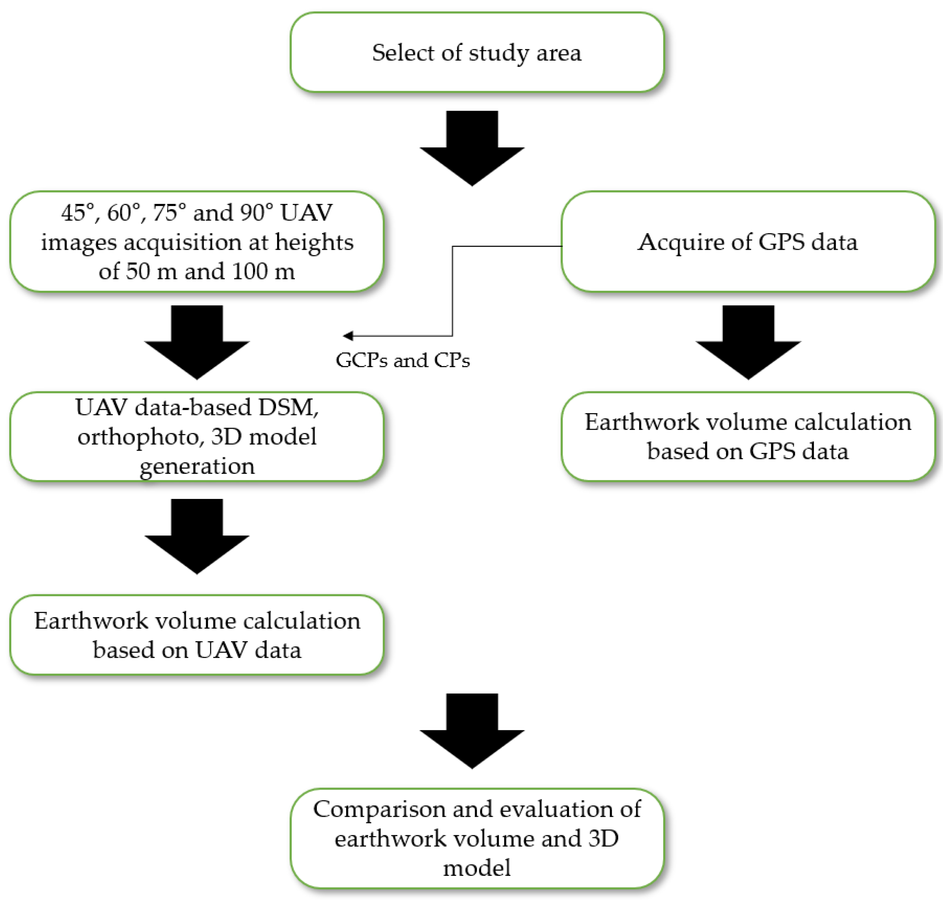
2. Materials and Methods
2.1. Study Area and Equipment
2.2. Data Acquisition and Method
2.2.1. UAV Data Acquisition
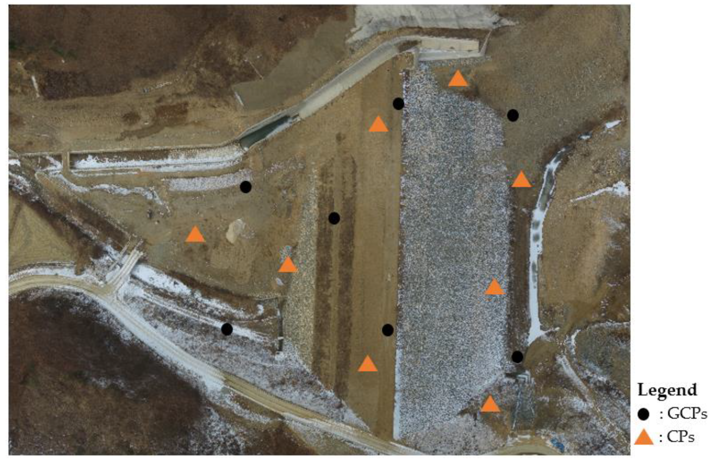
2.2.2. GPS Data Acquisition
2.2.3. Method
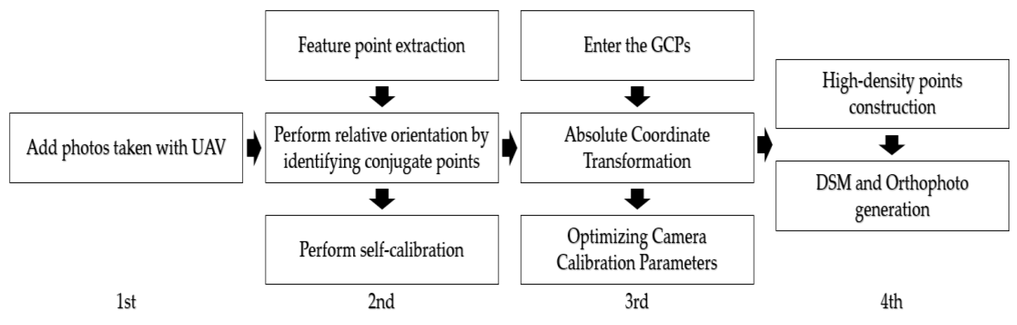
3. Image Processing
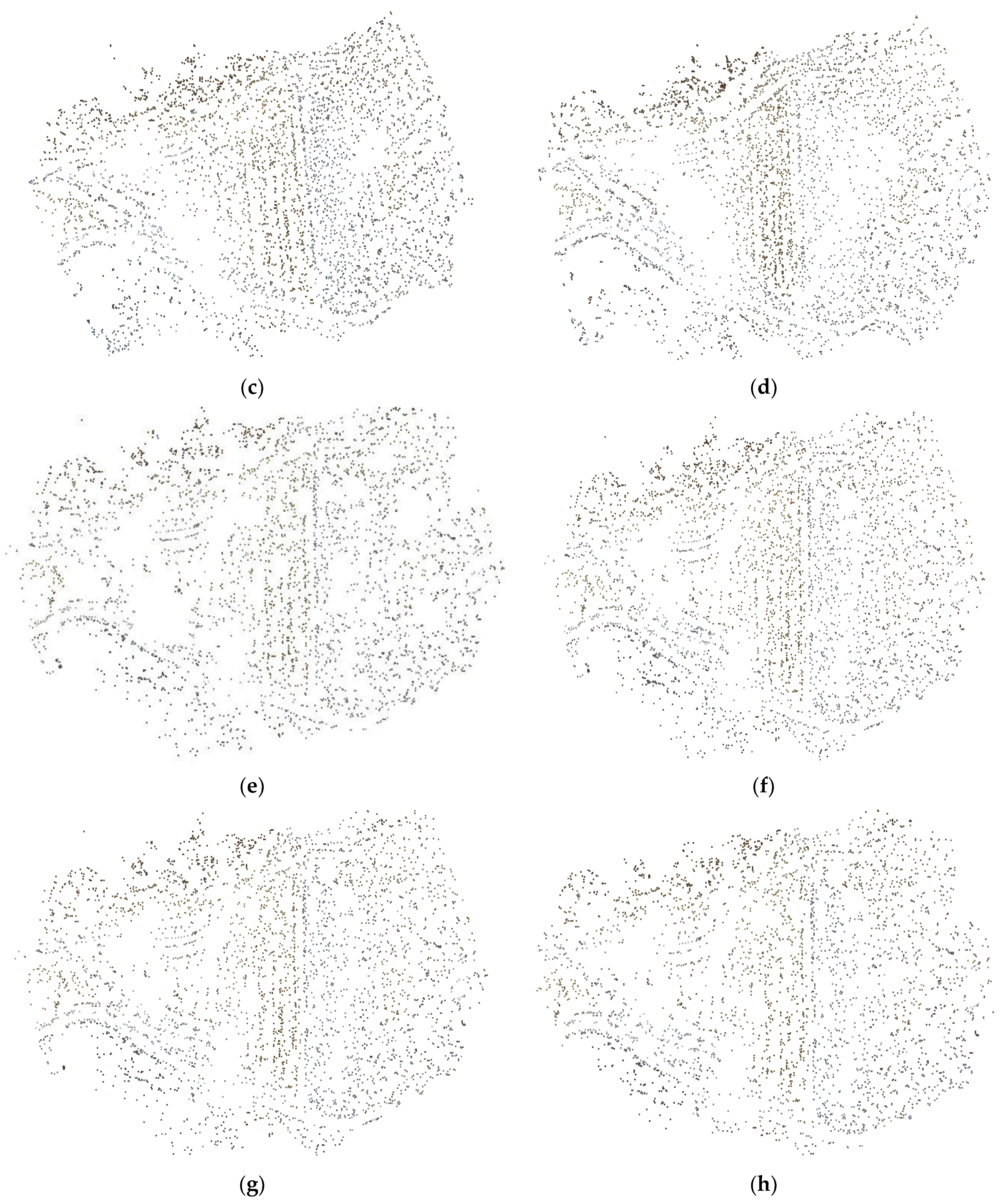
3.1. Image Matching
3.2. Camera Lens Distortion Correction
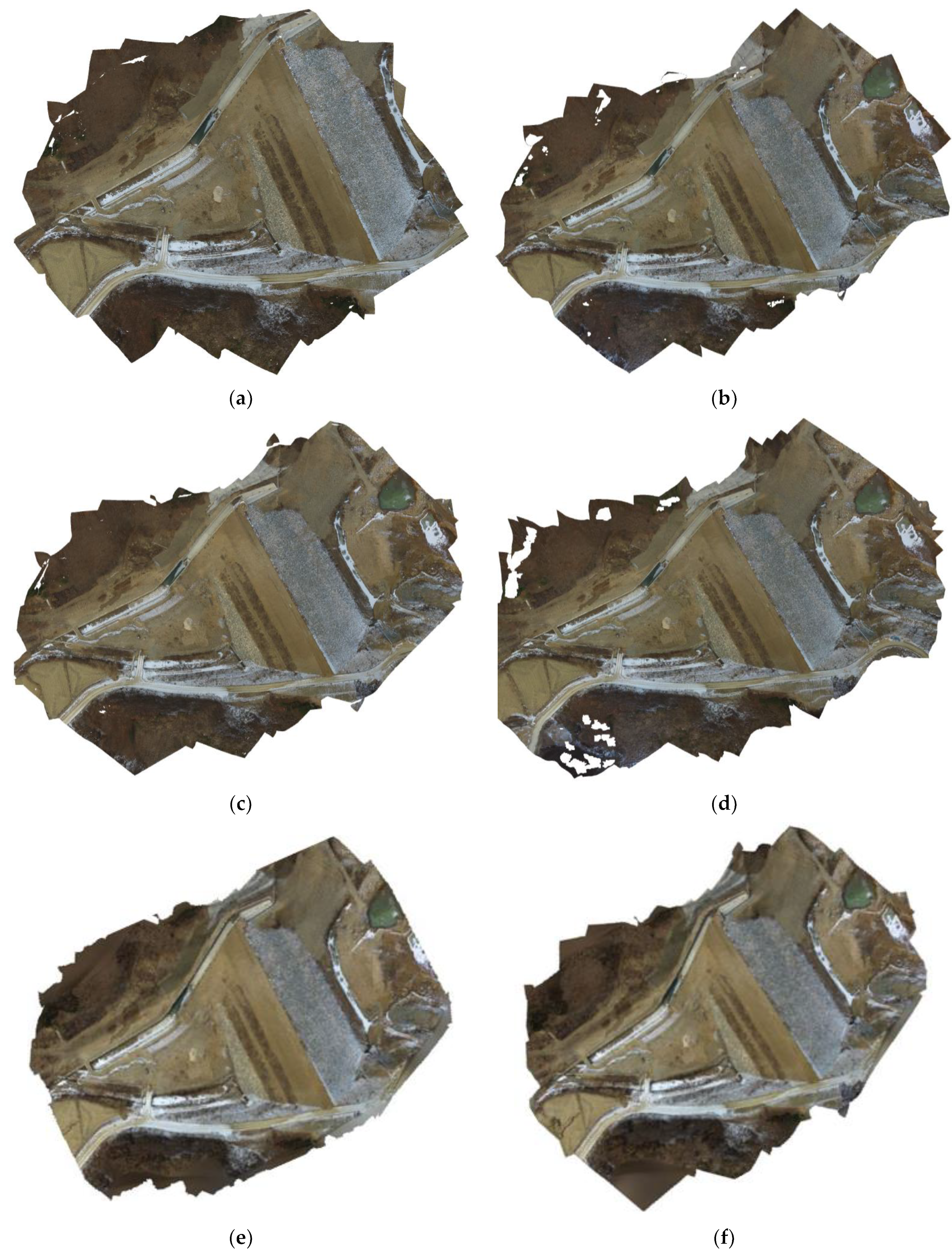
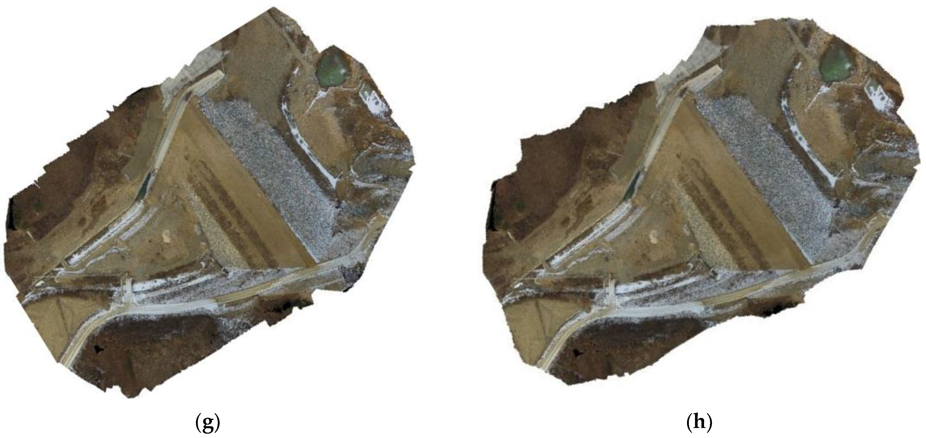
3.3. DSM and Orthophoto Generation
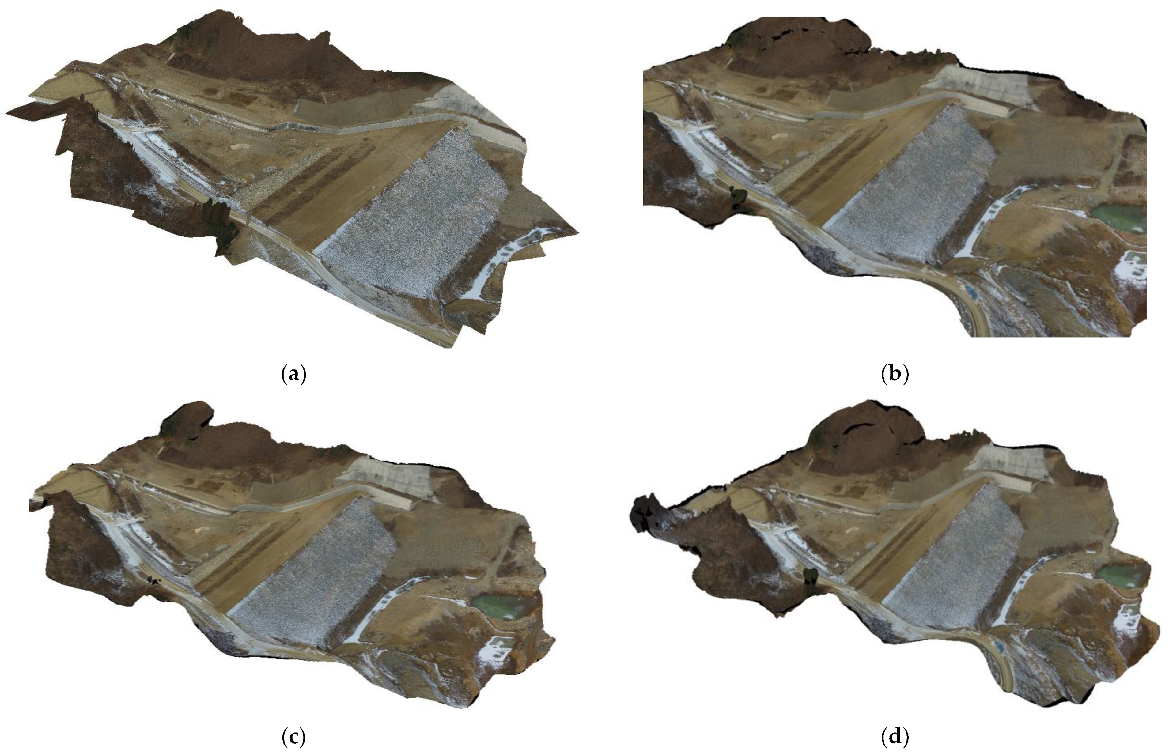
3.4. 3D Model Generation
3.5. Earthwork Volume Calculation
4. Results and Discussion
4.1. Orthophoto Accuracy Assessment
4.2. Earthwork Volume and 3D Model Accuracy Assessment
4.2.1. Earthwork Volume Accuracy Assessment
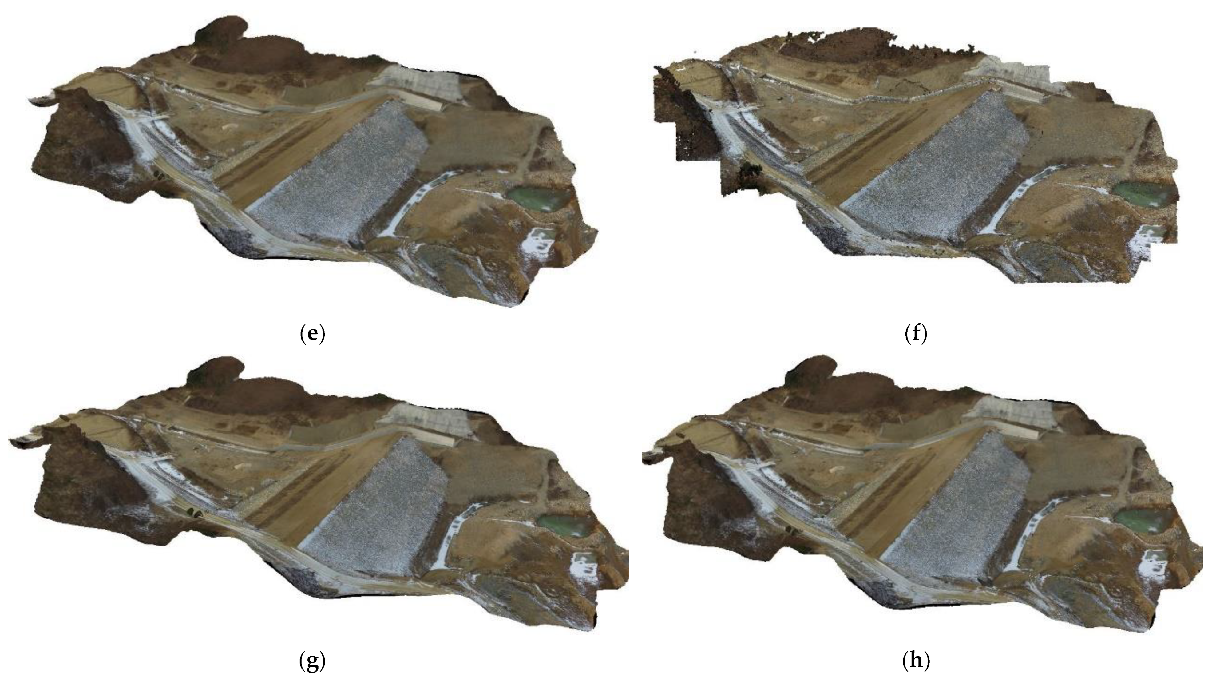
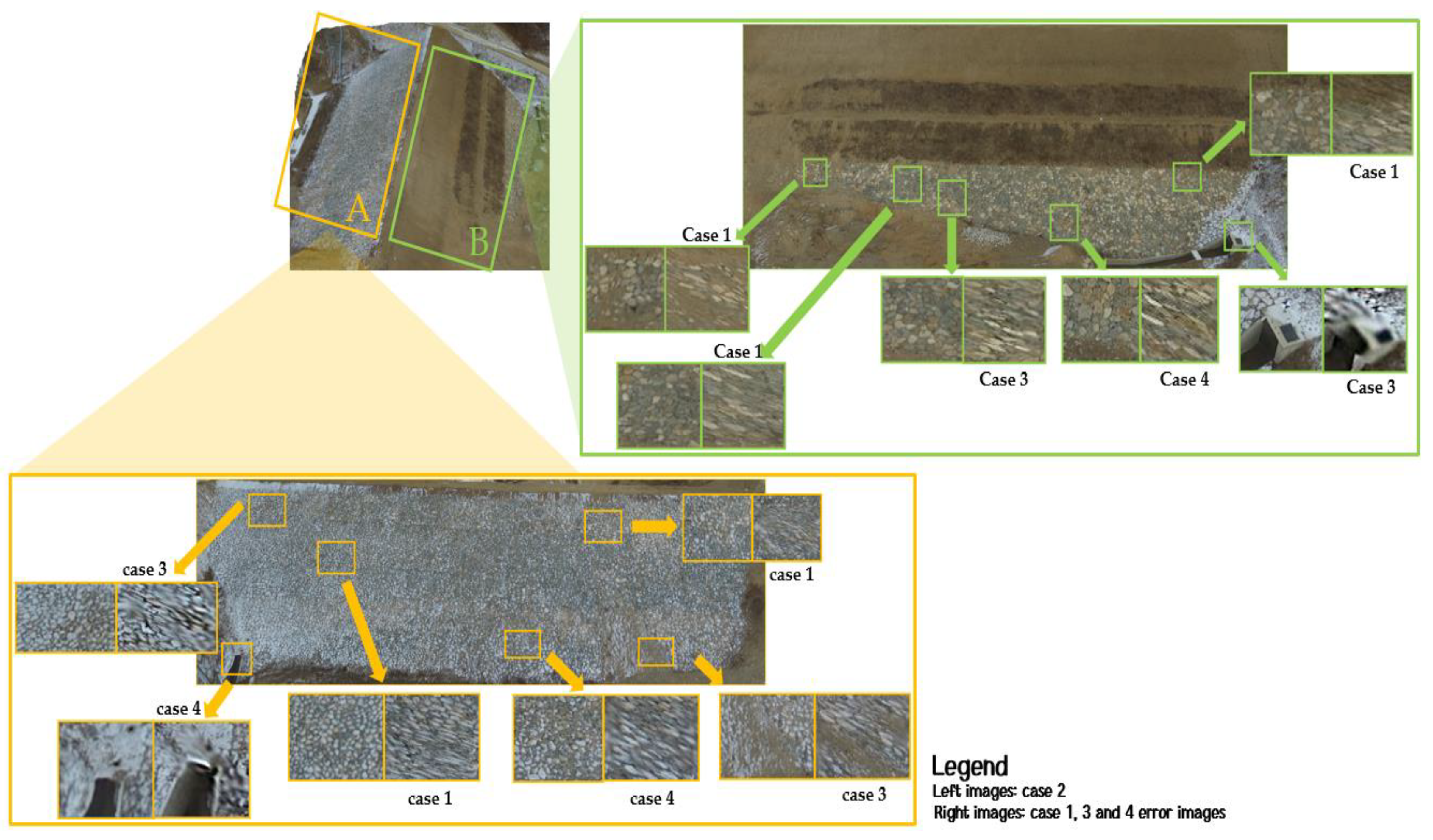
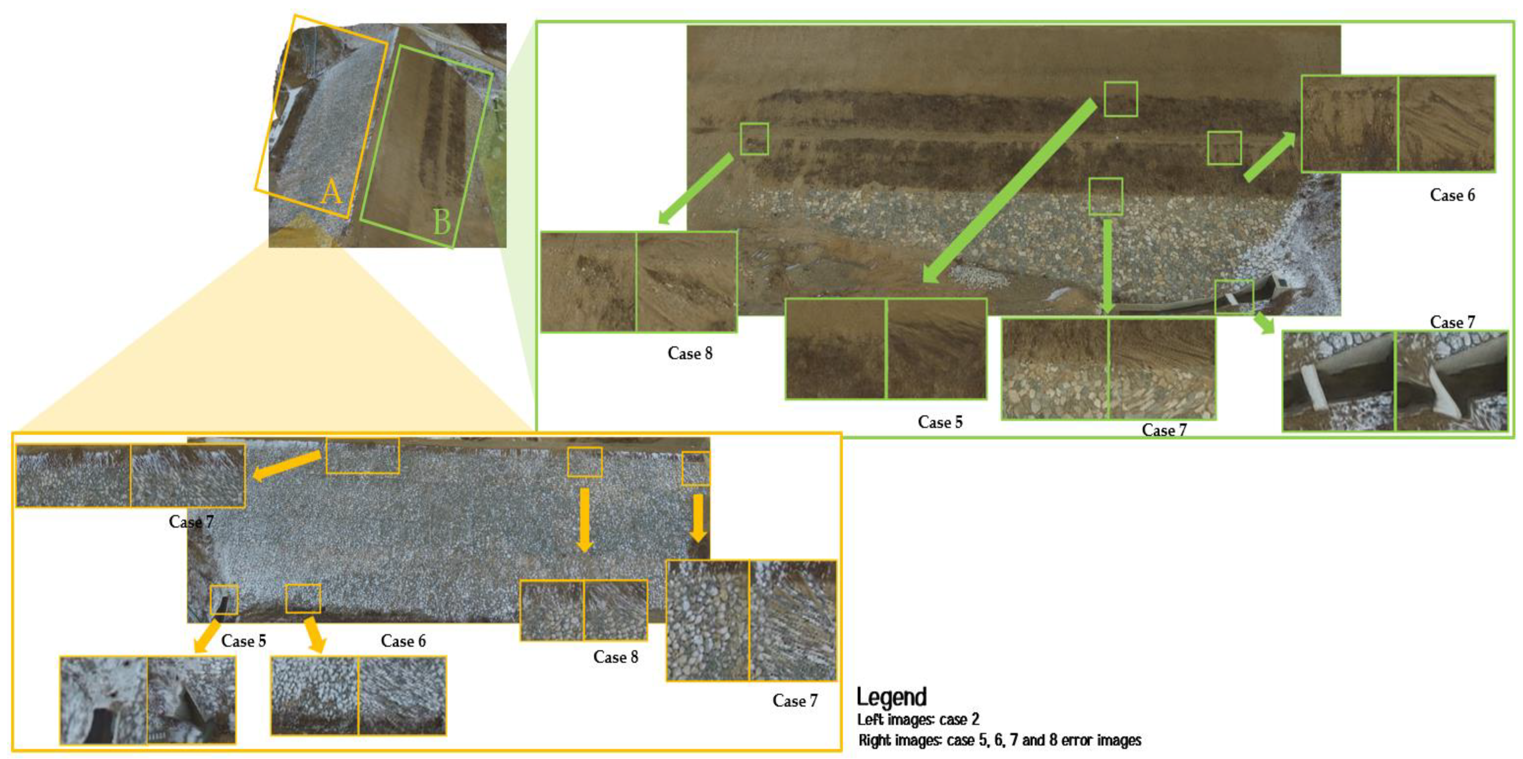
4.2.2. 3D Model Accuracy Assessment
5. Conclusions
Author Contributions
Funding
Data Availability Statement
Acknowledgments
Conflicts of Interest
References
- Akgul, M.; Yurtseven, H.; Gulci, S.; Akay, A.E. Evaluation of UAV- and GNSS-Based DEMs for Earthwork Volume. Arab. J. Sci. Eng. 2018, 43, 1893–1909. [Google Scholar] [CrossRef]
- Hugenholtz, C.H.; Walker, J.; Brown, O.; Myshak, S. Earthwork Volumetrics with an Unmanned Aerial Vehicle and Softcopy Photogrammetry. J. Surv. Eng. 2015, 141, 06014003. [Google Scholar] [CrossRef]
- Ali, F.A. Comparison among Height Observation of GPS, Total Station and Level and Their Suitability in Mining Works by Using GIS Technology. Int. Res. J. Eng. Technol. 2017, 4, 953–956. [Google Scholar]
- Abd-elqader, Y.S.; Fawaz, D.E.M.; Hamdy, A.M. Evaluation Study of GNSS Technology and Traditional Surveying in DEM Generation and Volumes Estimation. Aust. J. Basic Appl. Sci. 2020, 14, 18–25. [Google Scholar] [CrossRef]
- Seong, J.; Cho, S.I.; Xu, C.; Yun, H.C. UAV Utilization for Efficient Estimation of Earthwork Volume Based on DEM. J. Korean Soc. Surv. Geod. Photogramm. Cartogr. 2021, 39, 279–288. [Google Scholar] [CrossRef]
- Nesbit, P.R.; Hugenholtz, C.H. Enhancing UAV–SFM 3D Model Accuracy in High-relief Landscapes by Incorporating Oblique Images. Remote Sens. 2019, 11, 239. [Google Scholar] [CrossRef] [Green Version]
- Rossi, P.; Mancini, F.; Dubbini, M.; Mazzone, F.; Capra, A. Combining Nadir and Oblique UAV Imagery to Reconstruct Quarry Topography: Methodology and Feasibility Analysis. Eur. J. Remote Sens. 2017, 50, 211–221. [Google Scholar] [CrossRef] [Green Version]
- Zheng, J.; Yao, W.; Lin, X.; Ma, B.; Bai, L. An Accurate Digital Subsidence Model for Deformation Detection of Coal Mining Areas Using a UAV-Based LiDAR. Remote Sens. 2022, 14, 421. [Google Scholar] [CrossRef]
- Mello, C.C.D.S.; Salim, D.H.C.; Simões, G.F. UAV-based Landfill Operation Monitoring: A Year of Volume and TopoGraphic Measurements. Waste Manag. 2022, 137, 253–263. [Google Scholar] [CrossRef]
- Kameyama, S.; Sugiura, K. Estimating Tree Height and Volume using Unmanned Aerial Vehicle Photography and SfM Technology, with Verification of Result Accuracy. Drones 2020, 4, 19. [Google Scholar] [CrossRef]
- Demir, N.; Sönmez, N.K.; Akar, T.; Ünal, S. Automated Measurement of Plant Height of Wheat Genotypes using a DSM Derived from UAV Imagery. Proceedings 2018, 2, 350. [Google Scholar] [CrossRef]
- Lee, K.; Lee, W.H. Temperature Accuracy Analysis by Land Cover According to the Angle of the Thermal Infrared Imaging Camera for Unmanned Aerial Vehicles. ISPRS Int. J. Geo-Inf. 2022, 11, 204. [Google Scholar] [CrossRef]
- Jung, S.; Lee, W.H.; Han, Y. Change Detection of Building Objects in High-resolution Single-sensor and Multi-sensor Imagery Considering the Sun and Sensor’s Elevation and Azimuth Angles. Remote Sens. 2021, 13, 3660. [Google Scholar] [CrossRef]
- Jung, S.; Lee, K.; Yun, Y.; Lee, W.H.; Han, Y. Detection of Collapse Buildings Using UAV and Bitemporal Satellite Imagery. J. Korean Soc. Surv. Geod. Photogramm. Cartogr. 2020, 38, 187–196. [Google Scholar] [CrossRef]
- Cho, J.; Lee, J.; Park, J. Large-Scale Earthwork Progress Digitalization Practices Using Series of 3D Models Generated from UAS Images. Drones 2021, 5, 147. [Google Scholar] [CrossRef]
- Lee, K.R.; Lee, W.H. Comparison of Orthophoto and 3D Model Using Vertical and High Oblique Images Taken by UAV. J. Korean Soc. Geospat. Inf. Syst. 2017, 25, 35–45. [Google Scholar] [CrossRef]
- Seong, J.H.; Han, Y.K.; Lee, W.H. Earth-Volume Measurement of Small Area Using Low-Cost UAV. J. Korean Soc. Surv. Geod. Photogramm. Cartogr. 2018, 36, 279–286. [Google Scholar] [CrossRef]
- Ronchi, D.; Limongiello, M.; Barba, S. Correlation Among Earthwork and Cropmark Anomalies Within Archaeological Landscape Investigation by Using LiDAR and Multispectral Technologies from UAV. Drones 2020, 4, 72. [Google Scholar] [CrossRef]
- Kim, D.; Kim, S.; Back, K. Analysis of Mine Change Using 3D Spatial Information Based on Drone Image. Sustainability 2022, 14, 3433. [Google Scholar] [CrossRef]
- Kim, J.; Lee, S.; Seo, J.; Lee, D.; Choi, H.S. The Integration of Earthwork Design Review and Planning Using UAV-Based Point Cloud and BIM. Appl. Sci. 2021, 11, 3435. [Google Scholar] [CrossRef]
- Siebert, S.; Teizer, J. Mobile 3D Mapping for Surveying Earthwork Projects Using an Unmanned Aerial Vehicle (UAV) System. Autom. Constr. 2014, 41, 1–14. [Google Scholar] [CrossRef]
- Tucci, G.; Gebbia, A.; Conti, A.; Fiorini, L.; Lubello, C. Monitoring and Computation of the Volumes of Stockpiles of Bulk Material by Means of UAV Photogrammetric Surveying. Remote Sens. 2019, 11, 1471. [Google Scholar] [CrossRef] [Green Version]
- Filkin, T.; Sliusar, N.; Huber-Humer, M.; Ritzkowski, M.; Korotaev, V. Estimation of Dump and Landfill Waste Volumes using Unmanned Aerial Systems. Waste Manag. 2022, 139, 301–308. [Google Scholar] [CrossRef] [PubMed]
- Cho, S.I.; Lim, J.H.; Lim, S.B.; Yun, H.C. A Study on DEM-Based Automatic Calculation of Earthwork Volume for BIM Application. J. Korean Soc. Surv. Geod. Photogramm. Cartogr. 2020, 38, 131–140. [Google Scholar] [CrossRef]
- Grenzdörffer, G.J.; Guretzki, M.; Friedlander, I. Photogrammetric Image Acquisition and Image Analysis of Oblique Imagery. Photogramm. Record 2008, 23, 372–386. [Google Scholar] [CrossRef]
- Cheng, M.; Matsuoka, M. Extracting three-dimensional (3D) spatial information from sequential oblique unmanned aerial system (UAS) imagery for digital surface model. Int. J. Remote Sens. 2021, 42, 1643–1663. [Google Scholar] [CrossRef]
- Yang, B.; Ali, F.; Yin, P.; Yang, T.; Yu, Y.; Li, S.; Liu, X. Approaches for Exploration of Improving Multi-slice Mapping Via forWarding Intersection based on Images of UAV Oblique Photogrammetry. Comput. Electr. Eng. 2021, 92, 107135. [Google Scholar] [CrossRef]
- Vacca, G.; Dessì, A.; Sacco, A. The Use of Nadir and Oblique UAV Images for Building Knowledge. ISPRS Int. J. Geo-Inf. 2017, 6, 393. [Google Scholar] [CrossRef] [Green Version]
- Jiang, S.; Jiang, W. Efficient SfM for Oblique UAV Images: From Match Pair Selection to Geometrical Verification. Remote Sens. 2018, 10, 1246. [Google Scholar] [CrossRef] [Green Version]
- Zhang, X.; Zhao, P.; Hu, Q.; Ai, M.; Hu, D.; Li, J. A UAV-based Panoramic Oblique Photogrammetry (POP) Approach using Spherical Projection. ISPRS J. Photogramm. Remote Sens. 2020, 159, 198–219. [Google Scholar] [CrossRef]
- Bhatnagar, S.; Gill, L.; Ghosh, B. Drone image segmentation using machine and deep learning for mapping raised bog vegetation communities. Remote Sens. 2020, 12, 2602. [Google Scholar] [CrossRef]
- Zhu, W.; Sun, Z.; Huang, Y.; Yang, T.; Li, J.; Zhu, K.; Zhang, J.; Yang, B.; Shao, C.; Peng, J. Optimization of multi-source UAV RS agro-monitoring schemes designed for field-scale crop phenotyping. Precis. Agric 2021, 22, 1768–1802. [Google Scholar] [CrossRef]
- Ahmad, N.; Iqbal, J.; Shaheen, A.; Ghfar, A.; Al-Anazy, M.M.; Ouladsmane, M. Spatio-temporal analysis of chickpea crop in arid environment by comparing high-resolution UAV image and LANDSAT imagery. Int. J. Environ. Sci. Tech. 2022, 19, 6595–6610. [Google Scholar] [CrossRef]
- BN, P.K.; Chai, Y.H.; Patil, A.K. Inspired by Human Eye: Vestibular Ocular Reflex Based Gimbal Camera Movement to Minimize Viewpoint Changes. Symmetry 2019, 11, 101. [Google Scholar] [CrossRef] [Green Version]
- Lee, K.; Park, J.; Jung, S.; Lee, W. Roof Color-Based Warm Roof Evaluation in Cold Regions Using a UAV Mounted Thermal Infrared Imaging Camera. Energies 2021, 14, 6488. [Google Scholar] [CrossRef]
- Wanninger, L. Virtual Reference Stations (VRS). GPS Solut. 2003, 7, 143–144. [Google Scholar] [CrossRef]
- Park, J.; Lee, W. Orthophoto and DEM generation in small slope areas using low specification UAV. J. Korean Soc. Surv. Geod. Photogramm. Cartogr. 2016, 34, 283–290. [Google Scholar] [CrossRef] [Green Version]
- Elkhrachy, I. Accuracy assessment of low-cost Unmanned Aerial Vehicle (UAV) photogrammetry. Alex. Eng. J. 2021, 60, 5579–5590. [Google Scholar] [CrossRef]
- Han, S.; Park, J.; Lee, W. On-Site vs. Laboratorial Implementation of Camera Self- Calibration for UAV Photogrammetry. J. Korean Soc. Surv. Geod. Photogramm. Cartogr. 2016, 34, 349–356. [Google Scholar] [CrossRef] [Green Version]
- Zhu, G.; Wang, Q.; Yuan, Y.; Yan, P. SIFT on Manifold: An Intrinsic Description. Neurocomputing 2013, 113, 227–233. [Google Scholar] [CrossRef]
- Lowe, D.G. Distinctive Image Features from Scale-Invariant Keypoints. Int. J. Comput. Vis. 2004, 60, 91–110. [Google Scholar] [CrossRef]
- Han, Y.K.; Kim, Y.I.; Han, D.Y.; Choi, J.W. Mosaic Image Generation of AISA Eagle Hyperspectral Sensor Using SIFT Method. J. Korean Soc. Surv. Geod. Photogramm. Cartogr. 2013, 31, 165–172. [Google Scholar] [CrossRef] [Green Version]
- Mousavi, V.; Varshosaz, M.; Remondino, F. Using Information Content to Select Keypoints for UAV Image Matching. Remote Sens. 2021, 13, 1302. [Google Scholar] [CrossRef]
- Sun, Q.; Wang, X.; Xu, J.; Wang, L.; Zhang, H.; Yu, J.; Su, T.; Zhang, X. Camera Self-Calibration with Lens Distortion. Optik 2016, 127, 4506–4513. [Google Scholar] [CrossRef]
- Weng, J.; Zhou, W.; Ma, S.; Qi, P.; Zhong, J.; Lens, M.-F. Distortion Correction Based on Phase Analysis of Fringe-Patterns. Sensors 2021, 21, 209. [Google Scholar] [CrossRef] [PubMed]
- Jiang, J.; Zheng, H.; Ji, X.; Cheng, T.; Tian, Y.; Zhu, Y.; Cao, W.; Ehsani, R.; Yao, X. Analysis and Evaluation of the Image Pre-processing Process of a Six-Band Multispectral Camera Mounted on an Unmanned Aerial Vehicle for Winter Wheat Moni-toring. Sensors 2019, 19, 747. [Google Scholar] [CrossRef] [PubMed] [Green Version]
- Agisoft, L.L.C. Agisoft Metashape User Manual. Professional Edition, Version 1.7. 2021. Available online: http://www.agisoft.com/pdf/metashape-pro_1_7_en.pdf (accessed on 8 December 2021).
- Snavely, N.; Seitz, S.M.; Szeliski, R. Model the World from Internet Photo Collections. Int. J. Comput. Vis. 2008, 80, 189–210. [Google Scholar] [CrossRef] [Green Version]
- Rossi, G.; Tanteri, L.; Tofani, V.; Vannocci, P.; Moretti, S.; Casagli, N. Multitemporal UAV Surveys for Landslide Mapping and Characterization. Landslides 2018, 15, 1045–1052. [Google Scholar] [CrossRef] [Green Version]
- Mlambo, R.; Woodhouse, I.H.; Gerard, F.; Anderson, K. Structure from Motion (SfM) Photogrammetry with Drone Data: A Low Cost Method for Monitoring Greenhouse Gas Emissions from Forests in Developing Countries. Forests 2017, 8, 68. [Google Scholar] [CrossRef] [Green Version]
- Mosbrucker, A.R.; Major, J.J.; Spicer, K.R.; Pitlick, J. Camera System Considerations for Geomorphic Applications of SfM Photogrammetry. Earth Surf. Process. Landf. 2017, 42, 969–986. [Google Scholar] [CrossRef] [Green Version]
- Anderson, S.; Pitlick, J. Using Repeat Lidar to Estimate Sediment Transport in a Steep Stream. J. Geophys. Res. Earth Surf. 2014, 119, 621–643. [Google Scholar] [CrossRef]
- Cucchiaro, S.; Fallu, D.J.; Zhao, P.; Waddington, C.; Cockcroft, D.; Tarolli, P.; Brown, A.G. SfM Photogrammetry for Geoarchaeology. Dev. Earth Surf. Process. 2020, 23, 183–205. [Google Scholar] [CrossRef]
- Ferreira, E.; Chandler, J.; Wackrow, R.; Shiono, K. Automated Extraction of Free Surface Topography Using SfM-MVS Photogrammetry. Flow Meas. Instrum. 2017, 54, 243–249. [Google Scholar] [CrossRef] [Green Version]
- Lucieer, A.; Jong, S.M.d.; Turner, D. Mapping Landslide Displacements Using Structure from Motion (SfM) and Image Correlation of Multi-Temporal UAV Photography. Prog. Phys. Geogr. 2014, 38, 97–116. [Google Scholar] [CrossRef]
- Lee, K.R.; Lee, W.H. Orthophoto and DEM Generation Using Low Specification UAV Images from Different Altitudes. J. Korean Soc. Surv. Geod. Photogramm. Cartogr. 2016, 34, 535–544. [Google Scholar] [CrossRef] [Green Version]
- Lee, K.R.; Han, Y.K.; Lee, W.H. Comparison of Orthophotos and 3D Models Generated by UAV-Based Oblique Images Taken in Various Angles. J. Korean Soc. Surv. Geod. Photogramm. Cartogr. 2018, 36, 117–126. [Google Scholar] [CrossRef]
- Hao, X.; Pan, Y. Accuracy Analysis of Earthwork Calculation Based on Triangulated Irregular Network (TIN). Intell. Autom. Soft Comput. 2011, 17, 793–802. [Google Scholar] [CrossRef]
- Chen, Z.A.; Luo, Y.Y.; Zhang, L.T. Precision Analysis and Earthwork Computation of Land Consolidation Based on Surfer. Geotech. Investig. Surv. 2010, 5, 53–56. [Google Scholar]
- Kavaliauskas, P.; Židanavičius, D.; Jurelionis, A. Geometric Accuracy of 3D Reality Mesh Utilization for BIM-Based Earthwork Quantity Estimation Workflows. ISPRS Int. J. Geo-Inf. 2021, 10, 399. [Google Scholar] [CrossRef]
- Ajayi, O.G.; Oyeboade, T.O.; Samaila-Ija, H.A.; Adewale, T.J. Development of a UAV-Based System for the Semi-Automatic Estimation of the Volume of Earthworks. Rep. Geod. Geoinf. 2020, 110, 21–28. [Google Scholar] [CrossRef]
- Cho, J.; Lee, J.; Lee, B. A Study on the Optimal Shooting Conditions of UAV for 3D Production and Orthophoto Generation. J. Korean Soc. Surv. Geod. Photogramm. Cartogr. 2020, 38, 645–653. [Google Scholar] [CrossRef]
- Lee, K.R.; Han, Y.K.; Lee, W.H. Generation and Comparison of Orthophotos and 3D Models of Small-Scale Terraced Topography Using Vertical and High Oblique Images Taken by UAV. J. Korean Soc. Geospat. Inf. Sci. 2018, 26, 23–30. [Google Scholar] [CrossRef]


| UAV | RGB Camera | ||
|---|---|---|---|
| Inspire 1 | Zenmuse X3 | ||
| Weight | 2935 g | Resolution | 4000 × 3000 |
| Flight altitude | Max: 4500 m | Pixel size | 1.561 × 1.561 μm |
| Flight time | Max: 18 min | FOV | 94° |
| Speed | Max: 22 m/s | Focal length | 3.61 mm |
| Maximum wind resistance | 10 m/s | F-Stop | F/2.8 |
| GNSS Receiver | |
|---|---|
| Trimble R8s | |
| Weight | 3.81 kg |
| Number of channels | 440 channels |
| Satellite signal | GPS: L1C/A, L1C, L2C, L2E, L5 GLONASS: L1C/A, L1P, L2C/A, L2P, L3 SBAS: L1C/A, L5 (for SBAS satellites that support L5) Galileo: E1, E5A, E5B BeiDou: B1, B2 |
| VRS precision | Horizontal: 8 mm + 0.5 ppm RMS Vertical: 15 mm + 0.5 ppm RMS |
| Rules |
|---|
|
|
|
|
| GPS | Case 1 | Case 2 | Case 3 | Case 4 |
| 147,316.15 m3 | 149,214.71 m3 | 146,913.10 m3 | 144,681.48 m3 | 150,879.87 m3 |
| Case 5 | Case 6 | Case 7 | Case 8 | |
| 150,408.24 | 145,787.72 | 153,547.39 | 152,475.12 |
| GSD (cm) | RMSE (m) | Maximum Error (m) |
|---|---|---|
| Within 8 | 0.08 | 0.16 |
| Within 12 | 0.12 | 0.24 |
| Within 25 | 0.25 | 0.50 |
| Within 42 | 0.42 | 0.84 |
| Within 65 | 0.65 | 1.30 |
| Within 80 | 0.80 | 1.60 |
| GCP No. | Case 1 | Case 2 | Case 3 | Case 4 | ||||||||
|---|---|---|---|---|---|---|---|---|---|---|---|---|
| X | Y | Z | X | Y | Z | X | Y | Z | X | Y | Z | |
| 1 | −0.03 | 0.15 | −0.01 | 0.02 | −0.02 | 0.02 | −0.08 | 0.10 | 0.09 | 0.01 | 0.04 | 0.12 |
| 2 | 0.10 | 0.14 | 0.09 | −0.09 | −0.04 | 0.05 | −0.09 | 0.09 | −0.10 | 0.02 | 0.08 | 0.08 |
| 3 | 0.03 | 0.05 | −0.11 | 0.05 | −0.10 | −0.05 | −0.01 | −0.05 | −0.10 | 0.01 | 0.05 | −0.13 |
| 4 | −0.02 | −0.04 | −0.03 | −0.01 | 0.02 | 0.01 | −0.12 | −0.11 | −0.12 | 0.02 | 0.07 | −0.02 |
| 5 | −0.16 | 0.03 | 0.02 | −0.02 | 0.06 | −0.06 | 0.02 | 0.07 | 0.01 | 0.11 | −0.09 | −0.04 |
| 6 | 0.04 | 0.01 | 0.05 | 0.01 | −0.09 | −0.07 | 0.11 | 0.04 | 0.17 | −0.11 | 0.16 | 0.12 |
| 7 | 0.10 | 0.11 | 0.04 | −0.08 | 0.05 | −0.01 | −0.09 | 0.02 | −0.10 | 0.12 | 0.13 | −0.14 |
| 8 | −0.05 | 0.12 | −0.11 | 0.10 | 0.06 | 0.02 | −0.10 | 0.11 | 0.10 | −0.05 | 0.01 | 0.12 |
| RMSE | 0.08 | 0.07 | 0.07 | 0.06 | 0.06 | 0.04 | 0.08 | 0.08 | 0.11 | 0.07 | 0.07 | 0.11 |
| Maximum error | 0.10 | 0.15 | 0.09 | 0.10 | 0.06 | 0.05 | 0.11 | 0.11 | 0.17 | 0.12 | 0.16 | 0.12 |
| GCP No. | Case 5 | Case 6 | Case 7 | Case 8 | ||||||||
|---|---|---|---|---|---|---|---|---|---|---|---|---|
| X | Y | Z | X | Y | Z | X | Y | Z | X | Y | Z | |
| 1 | 0.12 | 0.10 | 0.10 | 0.03 | −0.08 | 0.05 | 0.11 | 0.06 | 0.12 | −0.08 | −0.06 | 0.09 |
| 2 | 0.11 | 0.10 | −0.04 | −0.05 | −0.04 | 0.08 | 0.11 | −0.06 | −0.08 | 0.05 | −0.09 | −0.09 |
| 3 | 0.01 | −0.03 | −0.10 | 0.02 | −0.04 | −0.04 | 0.08 | −0.08 | −0.10 | 0.12 | 0.09 | −0.10 |
| 4 | −0.05 | 0.02 | −0.04 | −0.07 | 0.04 | 0.02 | −0.08 | −0.12 | 0.12 | −0.02 | −0.08 | −0.11 |
| 5 | 0.10 | −0.09 | 0.09 | −0.09 | −0.06 | 0.06 | −0.05 | −0.07 | 0.10 | 0.11 | −0.09 | 0.11 |
| 6 | −0.10 | −0.02 | 0.06 | −0.02 | 0.10 | −0.05 | 0.09 | 0.06 | 0.12 | −0.12 | 0.13 | −0.10 |
| 7 | 0.08 | 0.10 | 0.07 | 0.02 | −0.03 | 0.02 | 0.05 | 0.05 | −0.10 | 0.10 | 0.11 | −0.12 |
| 8 | 0.10 | −0.10 | −0.09 | 0.09 | 0.06 | 0.02 | −0.09 | 0.10 | 0.13 | −0.09 | 0.06 | 0.13 |
| RMSE | 0.08 | 0.08 | 0.08 | 0.06 | 0.07 | 0.05 | 0.09 | 0.08 | 0.11 | 0.10 | 0.10 | 0.11 |
| Maximum error | 0.12 | 0.10 | 0.10 | 0.09 | 0.10 | 0.08 | 0.11 | 0.12 | 0.13 | 0.12 | 0.13 | 0.13 |
| Surveying Type | Accuracy | |
|---|---|---|
| GPS | 100% | |
| UAV | Case 1 | 98.71% |
| Case 2 | 99.73% | |
| Case 3 | 98.21% | |
| Case 4 | 97.58% | |
| Case 5 | 97.90% | |
| Case 6 | 98.96% | |
| Case 7 | 95.77% | |
| Case 8 | 96.50% | |
| Case 1 | Case 2 | Case 3 | Case 4 |
| ±0.11 m | ±0.05 m | ±0.09 m | ±0.14 m |
| Case 5 | Case 6 | Case 7 | Case 8 |
| ±0.12 m | ±0.07 m | ±0.13 m | ±0.16 m |
Publisher’s Note: MDPI stays neutral with regard to jurisdictional claims in published maps and institutional affiliations. |
© 2022 by the authors. Licensee MDPI, Basel, Switzerland. This article is an open access article distributed under the terms and conditions of the Creative Commons Attribution (CC BY) license (https://creativecommons.org/licenses/by/4.0/).
Share and Cite
Lee, K.; Lee, W.H. Earthwork Volume Calculation, 3D Model Generation, and Comparative Evaluation Using Vertical and High-Oblique Images Acquired by Unmanned Aerial Vehicles. Aerospace 2022, 9, 606. https://doi.org/10.3390/aerospace9100606
Lee K, Lee WH. Earthwork Volume Calculation, 3D Model Generation, and Comparative Evaluation Using Vertical and High-Oblique Images Acquired by Unmanned Aerial Vehicles. Aerospace. 2022; 9(10):606. https://doi.org/10.3390/aerospace9100606
Chicago/Turabian StyleLee, Kirim, and Won Hee Lee. 2022. "Earthwork Volume Calculation, 3D Model Generation, and Comparative Evaluation Using Vertical and High-Oblique Images Acquired by Unmanned Aerial Vehicles" Aerospace 9, no. 10: 606. https://doi.org/10.3390/aerospace9100606