Multi-Objective Optimization of Low Reynolds Number Airfoil Using Convolutional Neural Network and Non-Dominated Sorting Genetic Algorithm

Abstract

The airfoil is the prime component of flying vehicles. For low-speed flights, low Reynolds number airfoils are used. The characteristic of low Reynolds number airfoils is a laminar separation bubble and an associated drag rise. This paper presents a framework for the design of a low Reynolds number airfoil. The contributions of the proposed research are twofold. First, a convolutional neural network (CNN) is designed for the aerodynamic coefficient prediction of low Reynolds number airfoils. Data generation is discussed in detail and XFOIL is selected to obtain aerodynamic coefficients. The performance of the CNN is evaluated using different learning rate schedulers and adaptive learning rate optimizers. The trained model can predict the aerodynamic coefficients with high accuracy. Second, the trained model is used with a non-dominated sorting genetic algorithm (NSGA-II) for multi-objective optimization of the low Reynolds number airfoil at a specific angle of attack. A similar optimization is performed using NSGA-II directly calling XFOIL, to obtain the aerodynamic coefficients. The Pareto fronts of both optimizations are compared, and it is concluded that the proposed CNN can replicate the actual Pareto in considerably less time.

1. Introduction

Airfoil design is the most important part of flight vehicle design and requires considerable attention. Different airfoils have different aerodynamic characteristics that directly affect flight performance. The designed airfoil must exhibit acceptable performance in cruise conditions. The tools available for airfoil design are wind tunnel, CFD, and panel methods. Wind tunnel experimentation gives the most accurate results but has a high operating cost. CFD solvers compute the flow field around the airfoil using Navier–Stokes equations but require considerable time. Panel method codes give results in minimum time, but the results must be carefully checked and validated.

Progressive advancements in machine learning algorithms has led to their wide use in classification [1], numerical prediction [2], and pattern recognition [3]. Application of these algorithms in the fields of biology [4], engineering [5,6], environmental analysis [7], and medicine [8,9] marks their success. These algorithms learn from input data and make predictions for new unseen data. With the huge volume of available data [10,11,12] and the availability of high-performance GPUs (graphics processing units), the potentials of these algorithms are currently being tested as never before.

Recently, many researchers have applied these techniques in the field of aerospace. Ling et al. [13] applied three different machine learning algorithms to identify the regions of high Reynolds-averaged Navier–Stokes (RANS) uncertainties. Cruz et al. [14] replaced the Reynolds stress tensor by its divergence as a target for machine learning techniques to increase the fidelity of RANS modeling. Turbulence was predicted around subsonic airfoils using an artificial neural network (ANN) with great accuracy [15]. However, limited airfoils and free-stream conditions were considered. Bhushan et al. [16] explored the potential of machine learning to predict turbulence for oscillating plane channel flows. A stand-alone turbulence model was developed and the effects of input parameter selection and training approaches on the accuracy were investigated. Tao and Sun [17] developed a multi-fidelity surrogate-based optimization framework using a deep belief network (DBN) as the low-fidelity model and computational fluid dynamics (CFD) as the high-fidelity model. The proposed framework was embedded into particle swarm optimization (PSO) and applied to the robust optimization of transonic airfoils and wings, with the uncertainty in the Mach number. It was concluded that with an increase in iterations, the multi-fidelity surrogate predictions become very close to the CFD results. Azabi et al. [18] presented multi-objective optimization combined with ANN and applied it for the optimization of an unmanned aerial vehicle (UAV). Nine design variables were considered to define the UAV geometry. The optimized configuration showed an increase of 6.14% in endurance ratio in comparison with the base design. Xinghui et al. [19] optimized the wing and fin of a supersonic missile for maximum lift-to-drag ratio, using reinforcement learning (RL) and transfer learning (TL). Eight design variables were considered to define the canard. First, RL was used with DATCOM as aerodynamic prediction software to gain optimization experience. Subsequently, TL was used to resume optimization experience with CFD-based evaluation. The optimized configuration showed an increase of 18.67% in the lift-to-drag ratio with 62.5% lower CFD calls.

Similar design studies can be found regarding airfoil design and analysis. Saakaar et al. [20] used a convolutional network to predict the flow field around airfoils. Training data were generated using RANS simulations, but only three airfoils were considered for training. Vinothkumar et al. [21] used a multi-layer perceptron (MLP) to predict the flow field around 110 NACA airfoils at various angles of attack. OpenFOAM was used to generate data for training. For each case, 12,000 data points were selected from the region around the airfoil for computation of flow parameters. With an elapsed training time of more than two months, the trained model had an accuracy of 99% and 97% for training and test samples, respectively. Haizhou et al. [22] predicted the pressure field around transonic airfoils using a convolutional network. Training data contained 500 RAE2822 airfoils modified using the Hicks–Henne method. The trained model accurately predicted the shock wave and showed the ability to model non-linear flow. Sekar et al. [23] presented an inverse design for an airfoil using deep CNN. The training dataset consisted of over 1300 airfoils, but only one angle of attack was considered. An inverted grey image of the pressure distribution obtained from XFOIL was used as an input. The trained network showed good generalization performance in predicting test samples. A similar study was also presented by Yilmaz [24] for a single Reynolds number and zero angle of attack. Data were generated from the UIUC airfoil database and XFOIL. Different CNN architectures were studied along with optimization routines, layer arrangements, batch normalization, dropout, and learning rate. The average test accuracy for all prediction locations on the airfoil was approximately 80%.

Santos et al. [25] presented an MLP network to predict the aerodynamic coefficients of airfoils. XFOIL was used to generate aerodynamic data for subsonic conditions. Two different datasets were used, one with 10,000 airfoils and the other with 2,000 airfoils, to predict the stall angle and lift curve, respectively. The model showed considerable deviation at negative angles of attack. Haryanto et al. [26] used ANN to predict aerodynamic coefficients using the Joukowski transformation for airfoil representation. CFD was used to generate aerodynamic data. The trained network was used to optimize the airfoil for the maximum lift-to-drag ratio using a genetic algorithm. The performance of the optimized airfoil was validated using CFD and the error was 6%. Zhang et al. [27] proposed CNN to predict the airfoil lift coefficient. A total of 133 airfoils were considered, including symmetric airfoils and NACA 4- and 6-digit series airfoils. XFOIL was used to obtain the corresponding lift coefficients for a wide range of angles of attack, Reynolds numbers, and Mach numbers. The trained model showed comparable performance with MLP in learning capabilities. Yilmaz et al. [28] predicted the pressure distribution on airfoils. A total of 1562 airfoils were considered, and aerodynamic data were generated using an in-house panel method code. The structures of the softmax classifier, the combination of autoencoders with hidden layers and the CNN were discussed, and it was concluded that the CNN outperformed other networks by achieving more than 80% test accuracy. Zhelong et al. [29] also used CNN for aerodynamic coefficient prediction of airfoils using the signed distance function (SDF) for airfoil representation. Around 5000 airfoils were generated from NACA 63-215 airfoil, using 10 Hicks–Henne bump functions, and XFOIL was used to generate aerodynamic data. Compared with the Kriging surrogate model, CNN significantly improved the prediction accuracy with less than 5% error. A similar study was presented for pressure distribution prediction [30]. Latin hypercube sampling (LHS) and free-form deformation were used to generate 1500 variants of the RAE 2822 airfoil. The SDF was used for airfoil representation and CFD was used for data generation for a single Reynolds number and angle of attack. The trained model showed an accuracy of 97% and 94% for lower and upper surfaces, respectively. Chen et al. [31] introduced the concept of the transformed airfoil image (TAI) with CNN for predicting multiple aerodynamic coefficients of airfoils. A total of 6561 airfoils were generated from NACA 0012 using the Hicks–Henne bump function. CFD was used to generate data for 300 airfoils for multiple angles of attack and Mach numbers. TAI images of 85 × 85 pixels were used as input. The trained model showed a lower root mean square error (RMSE) compared to directed acyclic graph (DAG) and MLP methods.

In the current study, the potential of CNN was explored to predict the performance of low Reynolds number airfoils. Low Reynolds number airfoils are characterized by their associated laminar separation bubble. Due to an adverse pressure gradient, the laminar flow fails to make a transition to turbulent flow in the attached boundary layer and detaches from the surface. A laminar-to-turbulent transition occurs in the detached shear layer and a laminar separation bubble is formed when the turbulent flow is re-attached to the surface. The drag polar and transition locations for the E387 airfoil at a Reynolds number of 2.0 × 10⁵ are shown in Figure 1. There is a range of lift coefficients for which the drag coefficient remains almost constant or increases only slightly (points 1 and 2). In this range, the transition curve is steep, i.e., the transition moves towards the leading edge very slowly. Afterward, there is a sudden increase in the drag coefficient. This is because the associated transition locations move upstream abruptly.

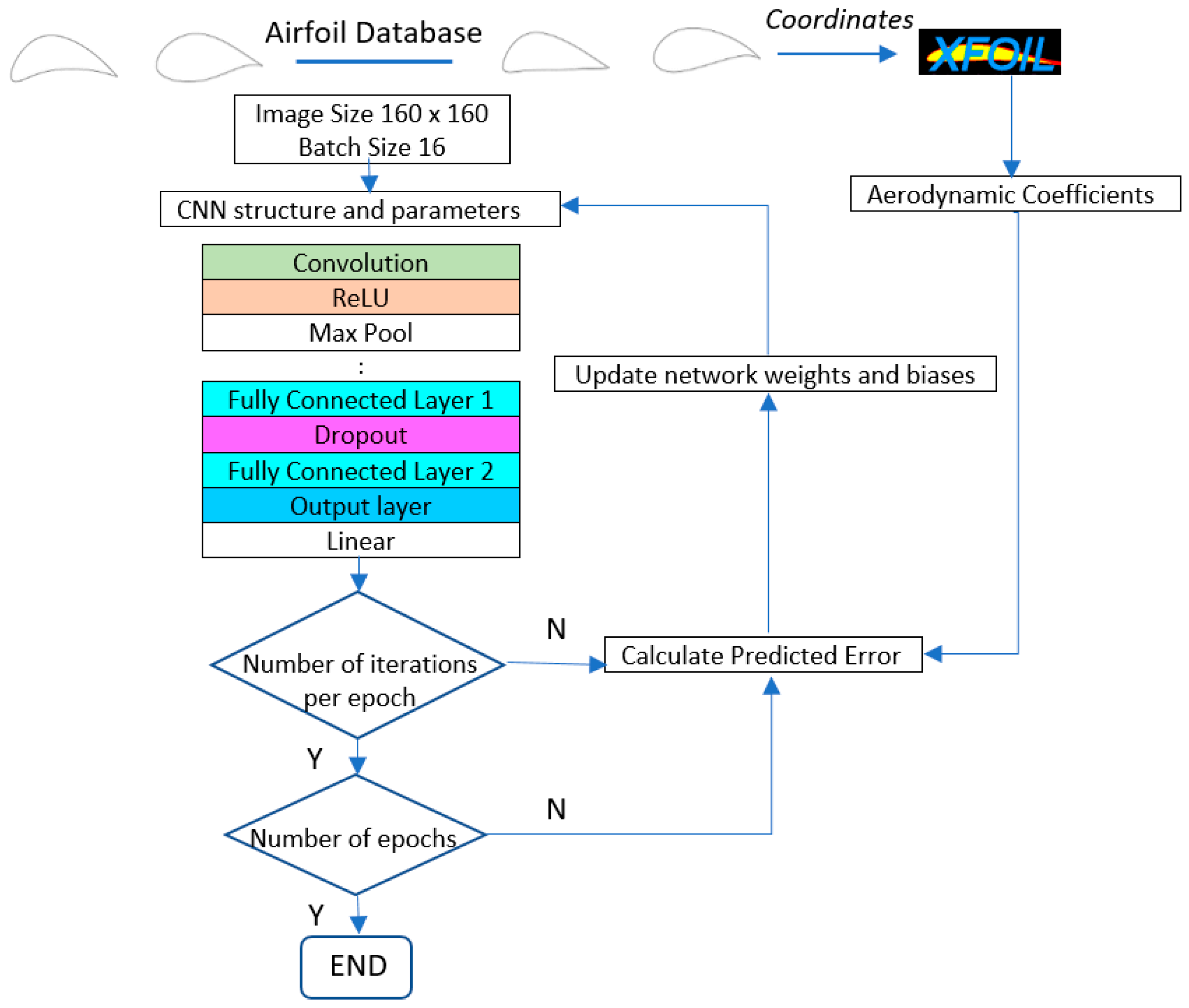
A detailed study was conducted for aerodynamic data generation using CFD and XFOIL. XFOIL was selected for the current study as it gives reasonably good results in less time. To generate the airfoil database, CST parameters of various low Reynolds number airfoils were used. Greyscale images of airfoils of size 160 × 160 pixels were used as input for the proposed CNN. The proposed CNN has five consecutive convolutional and pooling pairs with two fully connected layers. Several optimizers were tested to obtain the best model for predicting 48 aerodynamic coefficients. The trained CNN network had the capability to predict aerodynamic coefficients with high accuracy. This network was then used for multi-objective optimization of the airfoil for a specific alpha using NSGA-II. Similar multi-objective optimization was also performed using NSGA-II and XFOIL. The Pareto fronts of both optimizations were compared for validation and accuracy. The rest of the paper is organized as follows. Section 2 gives a general theoretical and structural discussion about neural networks and optimizers. Data generation is discussed in Section 3. The proposed CNN structure is presented in Section 4. The predicted results and further discussion are presented in Section 5. Section 6 presents a few conclusions, followed by the References section.

2. Machine Learning Methods

Machine learning refers to the branch of computer algorithms that learn from training data, extract features, generalize, and apply the results to test data. One machine learning algorithm that is widely used in the fields of autonomous exploration, speech recognition, and medical image analysis is deep learning [32,33,34]. In deep learning, the CNN has proven very effective in analyzing visual imagery. The main advantage of a CNN is that it can reduce the size of the image without losing essential features that are required for good predictions.

A CNN can be divided into two parts, i.e., feature extraction and classification. Feature extraction consists of convolutional layers and pooling layers. The convolutional layers are used to extract features. The purpose of the pooling layer is to reduce the spatial size of the convolved features. The second part of the CNN is the classification. This part consists of multiple fully connected layers. The input of these layers consists of non-linear combinations of high-level features. The output is the probability of the input image being in a specific class in the case of a classification problem or a scalar value in the case of a regression problem.

In order to learn complex patterns in the data, activation functions are added in neural networks. The activation function can be linear or non-linear. The output of a linear activation function is simply the weighted sum of the inputs, and backpropagation cannot be applied. Non-linear activation functions in neural networks introduce non-linear capabilities and also address the problems of linear activation functions. The details of the most commonly used activation functions are presented in

Table 1. Activation functions in CNN.

Function	Linear	Sigmoid	Tanh	ReLU
Formula	$y=ax$	$y=1/\left(1+e^{-x}\right)$	$y=\frac{e^x-e^{-x}}{e^x+e^{-x}}$	$y=\max \left(0,x\right)$
Nature	Linear	Non-Linear	Non-Linear	Non-Linear
Range	[−inf inf]	[0 1]	[−1 1]	[0 inf]
Response

.

The CNN model uses an optimizer to change parameters such as weights and learning rate to minimize the loss function. Gradient descent is the most basic optimization algorithm. The gradient of the loss function with respect to the parameters is calculated, and the parameters are updated using backpropagation. Hence, the parameter update rule is given by Equation (1).

$${\theta }_{t+1}={\theta }_t-\eta d_t$$

(1)

where $d_t$ represents the gradient of objective function $J\left(\theta \right)$ based on parameter $\theta$ at time $t$ and $\eta$ is the learning rate. Variants of gradient descent are stochastic gradient descent (SGD) and mini-batch gradient descent. The challenge in gradient descent methods is choosing the optimum value of the learning rate. A small learning rate requires more training epochs, whereas a large learning rate can cause the network to quickly converge to a suboptimal solution.

An alternate option is adaptive learning rate methods. The most commonly used methods are AdaGrad, RMSprop and Adam. AdaGrad assigns a small learning rate to parameters associated with frequently occurring features and a high learning rate to parameters associated with infrequent features. The parameter update rule for AdaGrad is given by Equation (2).

$${\theta }_{t+1}={\theta }_t-\frac{\eta }{\sqrt{D_t+ϵ}}{d}_t$$

(2)

where $D_t$ is a diagonal matrix. Each element of this matrix is the sum of squared gradients with respect to the parameter $\theta$ at time $t$. In addition, $ϵ$ is a vector of small numbers to avoid division by zero. The problem with AdaGrad is that for dense features, the learning rate decreases rapidly to the point where the algorithm is unable to acquire additional knowledge. RMSprop is introduced to address AdaGrad’s monotonically decaying learning rate. The RMSprop weight update rule divides the learning rate by the square root of the exponentially decaying average of squared gradients $R{\left[d^2\right]}_t$. The weight update rule is given by Equation (3).

$${\theta }_{t+1}={\theta }_t-\frac{\eta }{\sqrt{R{\left[d^2\right]}_t+ϵ}}{d}_t$$

(3)

The Adam optimizer keeps the exponentially decaying average of the past squared gradients (first moment) and the exponentially decaying average of past gradients (second momentum).

$$m_t={\beta }_1{m}_{t-1}+\left(1-{\beta }_1\right)d_t$$

(4)

$$v_t={\beta }_2{v}_{t-1}+\left(1-{\beta }_2\right)d_t^2$$

(5)

Here, $m_t$ and $v_t$ are estimates of the first moment (the mean) and second moment (variance) of the gradients, respectively, and ${\beta }_1$ and ${\beta }_2$ are very small numbers. In addition, $m_t$ and $v_t$ are biased towards zero when the decay rates are very small. To overcome this bias, the corrected $m_t$ and $v_t$ are given by

$${\widehat{m}}_t=\frac{m_t}{1-{\beta }_1^t}$$

(6)

$${\widehat{v}}_t=\frac{v_t}{1-{\beta }_2^t}$$

(7)

The parameter update rule for the Adam optimizer is given by Equation (8).

$${\theta }_{t+1}={\theta }_t-\frac{\eta }{\sqrt{{\widehat{v}}_t+ϵ}}{\widehat{m}}_t$$

(8)

3. Data Generation

CNN requires a large amount of data for the training data. Aerodynamic data for low Reynolds number airfoils can be obtained from wind tunnel experimentation, CFD, or panel method codes. It is not possible to perform experimentation on such a large scale. On the other hand, CFD requires considerable time. Panel method codes such as XFOIL can give results within seconds. This section presents a detailed aerodynamic analysis to ensure that the data used for CNN training have high accuracy.

The classical validation case for low Reynolds number airfoil data is E387 at a Reynolds number of 2.0 × 10⁵. Experimental data can be found in [35]. CFD analysis requires grid study and solver settings. Ansys ICEM was used to generate a C-H grid around the airfoil. Four grids were studied to ensure that the selected grid was fine enough to capture the laminar separation bubble and associated flow physics. The grid study was performed for an alpha of 4°. The details of grids and the corresponding lift and drag coefficients are presented in

Table 2. Grid study of E387 at Reynolds number 2.0 × 10⁵.

Grid	Size	${\mathit{c}}_{\mathit{l}}$	${\mathit{c}}_{\mathit{d}}$	Residuals
1	46,042	0.794	0.0131	1 × 10−4
2	69,192	0.794	0.0132	1 × 10−4
3	96,742	0.796	0.0132	1 × 10−5
4	128,692	0.796	0.0132	1 × 10−5

. This analysis was carried out using Ansys Fluent pressure-based, steady, Transition SST, coupled pressure–velocity, and second-order upwind schemes for spatial discretization.

Lift and drag coefficients for all the grids were the same. The grid selection was made on the basis of the pressure coefficient distribution, as shown in Figure 2. The pressure coefficient distribution for grids 1 and 2 shows oscillation near the laminar separation. Grids 3 and 4 show no oscillation and match the experimental data. Hence, grid 3 was selected for further analysis.

The aerodynamic data of E387 were also generated using XFOIL [36]. For the XFOIL analysis, a value of 9 was used for Ncrit, which represents the standard turbulence level. Drag polar values obtained from CFD and XFOIL are compared in Figure 3 below.

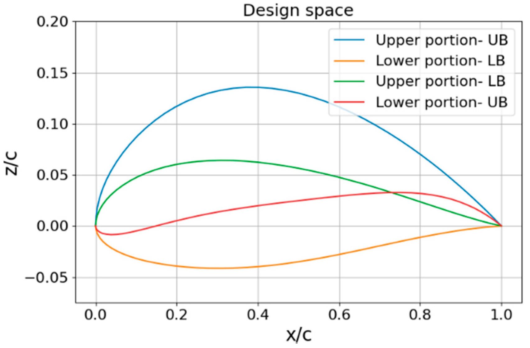
The results of CFD and XFOIL were in good agreement with experimental data, except for very high angles of attack. However, considering the time consumed in CFD simulation, XFOIL was selected for data generation. To generate the airfoil database, 15 low Reynolds number airfoils were considered. These airfoils are recommended for low-altitude solar-powered UAVs in the literature [37]. These airfoils were parameterized using CST, using a fourth-order polynomial, which gave ten parameters: five each for the lower and upper surfaces. For each parameter, the highest and lowest values of all the airfoils were used as the upper bound (UB) and lower bound (LB), respectively. The airfoil dataset was then created using Latin hypercube sampling (LHS). The entire design space using this UB and LB is shown in Figure 4.

The design spaces of the upper and lower portions overlap at the trailing edge. A constraint was applied to check the thickness of the airfoil. If the thickness was negative, the corresponding airfoil sample was discarded. An additional constraint was applied to ensure that the maximum thickness was between 9% and 14%. Aerodynamic data were generated for a Reynolds number of 0.17 × 10⁶, representing flight conditions of 9 m/s at an altitude of 800 m with a chord length of 0.3 m.

4. CNN Structure

The input of the proposed CNN was 160 × 160 greyscale images of the airfoils. A total of 3500 airfoils were generated using UB, LB, and LHS. After applying the thickness constraint and removing diverging airfoils, 2300 airfoils were used for training. Hence, 90% of the images were used for training and the remaining 10% were used for validation. The aerodynamic coefficients were normalized using the maximum and minimum values. The pixel values of the input images were also normalized. Five pairs of convolutional and pooling layers were used with the ReLU activation function. All convolutional layers had valid padding with a stride of 1. Other details of the convolutional layers are presented in

Table 3. Parameters for convolutional and pooling layers.

Layer	Filter Size	Pool Size	No. of Filters	Stride	Output Shape
Conv-1	5 × 5	---	64	1	(156, 156, 64)
Pool-1	---	2 × 2	---	2	(78, 78, 64)
Conv-2	3 × 3	---	128	1	(76, 76, 128)
Pool-2	---	2 × 2	---	2	(38, 38, 128)
Conv-3	3 × 3	---	256	1	(36, 36, 256)
Pool-3	---	2 × 2	---	2	(18, 18, 128)
Conv-4	3 × 3	---	256	1	(16, 16, 256)
Pool-4	---	2 × 2	---	2	(8, 8, 256)
Conv-5	3 × 3	---	512	1	(6, 6, 512)
Pool-5	---	2 × 2	---	2	(3, 3, 512)

. All pooling layers had 2 × 2 filters and a stride of 2. Two fully connected layers were applied after flattening. The first fully connected layer had 256 neurons and the second layer had 128 neurons. The output layer had 48 nodes with a linear activation function. These nodes corresponded to 16 lift, drag, and moment coefficients, respectively. A batch size of 16 was used with the mean squared error as the loss function. A dropout of 0.1 was applied between the fully connected layers. The Python language with the Keras deep learning API was used to set up this proposed CNN.

The training process for the proposed airfoil-CNN prediction model is shown in Figure 5. The number of iterations represents one batch of airfoils passing through the network during an epoch.

5. Results and Discussion

The proposed CNN was trained using several optimizers to obtain the best results in the minimum time. An SGD optimizer can be used with a constant, exponential, and step decay learning rate scheduler. Different learning rates and parameters were tried to obtain the optimum results.

Table 4. Convergence of SGD with constant, exponential, and step decay.

Learning Rate	Constant	Exp. Decay	Step Decay
Formula	$lr=cont$	$lr=l{r}_0\ast exp\left(-k\ast eph\right)$	$lr=l{r}_0\ast drop^\left(eph/ep{h}_{drp}\right)$
Parameters	$const=0.1$	$l{r}_0=0.15, k=0.0025$	$l{r}_0=0.1, drop=0.75, ep{h}_{drp}=80$
Loss Function

shows the convergence of the SGD with the constant, exponential, and step decay learning rate scheduler and associated parameters, where $lr$ is the learning rate, $l{r}_0$ is the initial learning rate, $drop$ is the percentage drop in $lr$, $eph$ is the epoch, $ep{h}_{drp}$ is the number of epochs after which $drop$ is applied, and $k$ is the hyperparameter.

The convergence and accuracies of all learning rate schedulers were almost the same. However, exponential and step decay show relatively smooth learning ability. For the first 400 epochs, MSE converges very fast. After that, features are only fine-tuned, and convergence is reduced. It is important to mention here that this level of convergence is achieved after extensive trial and error.

Three adaptive learning rate optimizers, AdaGrad, RMSprop, and Adam, were also considered for training. The initial learning rate was varied from 1 to 0.00001 for each optimizer. The RMS convergence for these optimizers is presented in

Table 5. Convergence of AdaGrad, RMSprop, and Adam.

Optimizer	AdaGrad	RMSprop	Adam
Parameters	$l{r}_0=0.1$	$l{r}_0=0.0001$	$l{r}_0=0.0001$
Loss Function

.

The MSE curves for AdaGrad, RMSprop, and Adam show oscillation, which means relatively higher weight updates. The order of convergence of these adaptive optimizers was the same as that of SGD. For all the optimizers, the training MSE was lower than the test MSE. This is because of dropout. Dropout randomly turns off neurons and makes prediction difficult for the network. Dropout is not applied to the test data. The selection of optimizers must be made considering the best output for particular input data. In [31], SGD with step decay was selected, whereas in [24], the performance of SGD was the worst. In our case, all optimizers show similar accuracy after parameter tuning. However, Adam was selected for further analysis as it may be the best optimizer for deep learning [19,21,23,28,29,30].

The predicted lift, drag, and moment coefficients for three random test airfoils are shown in Figure 6. The predicted results are in good agreement with the actual data. Hence, the trained network has the potential to predict aerodynamic coefficients with high accuracy.

For all the training and test airfoils, a comparison of predicted and actual aerodynamic coefficients is shown in Figure 7. It can be seen that most of the data points are clustered near a 45° line, indicating that predicted values are very close to actual values. Drag data are a little scattered at higher angles of attack. Drag prediction can be improved by adding more airfoils for training.

The trained CNN was used to design an airfoil using NSGA-II. NSGA-II is a multi-objective optimization method that searches for Pareto optimal solutions in the design space with high convergence speed. NSGA-II creates a parent population $P_t$ of size $N$. An offspring population $Q_t$ of the same size is created from $P_t$ using cross-over and mutation functions. Every individual in both populations is then ranked based on their fitness value. Every individual is then compared with all the other individuals in pairs to check for dominance and the number of dominations. Accordingly, individuals are classified into different Paretos. This process is called non-dominated sorting. The Pareto front can now be formed by individuals with zero domination count, i.e., they are not dominated by any other individual. A new population is then created using the individuals from the best fronts until the specified size ($N$) is reached. The population size, generation, cross-over probability, and mutation probability were set at 200, 40, 0.9, and 0.1, respectively. The optimization problem is defined as:

$$\begin{gathered} Min. f_1\left(x\right)=c_l \\ Min. f_2\left(x\right)=\frac{1}{c_l/c_d} \\ L{B}_i\le x_i\le U{B}_i i=1, . . . ,10 \end{gathered}$$

(9)

where $c_l$ and $c_d$ are lift and drag coefficients, respectively. The optimization problem is also set up in Python using $pymoo$. In pymoo, each objective function is supposed to be minimized. Hence, the drag-to-lift ratio is selected as the objective function instead of the lift-to-drag ratio. This multi-objective optimization was also performed using NSGA-II and XFOIL. Here, NSGA-II directly calls XFOIL for aerodynamic coefficients. The purpose of this was to compare the CNN predictions with XFOIL for a wider range of airfoil shapes and corresponding aerodynamic coefficients. The angle of attack considered for this study was 4.5°. The Pareto fronts for both NSGA-II with CNN and NSGA-II with XFOIL optimization are shown in Figure 8. Dominated solutions for NSGA-II with CNN are also plotted.

From Figure 8, it is clear that the Pareto fronts overlap each other, except for a lift coefficient of 0.6 to 0.7. Hence, more training airfoils are required that operate at this lift coefficient range at an alpha of 4.5°. Overall, CNN exhibits very good prediction accuracy. Eight airfoils were selected from the NSGA-II with CNN Pareto front for further analysis, corresponding to lift coefficients of 0.5, 0.6, 0.7, 0.8, 0.9, 1.0, 1.1, and 1.2. The objective function values, lift-to-drag ratios $c_l/c_d$, maximum thickness-to-chord ratios $t/c_{max}$, location of maximum thickness $x_{t/c_{max}}$, and airfoil shapes are shown in

Table 6. Details of selected airfoils for NSGA-II with CNN.

${\mathit{f}}_1\left(\mathit{x}\right)$	${\mathit{f}}_2\left(\mathit{x}\right)$	${\mathit{c}}_{\mathit{l}}/{\mathit{c}}_{\mathit{d}}$	$\mathit{t}/{\mathit{c}}_{\mathit{m}\mathit{a}\mathit{x}}$	${\mathit{x}}_{\mathit{t}/{\mathit{c}}_{\mathit{m}\mathit{a}\mathit{x}}}$	Airfoil Shape
0.515	0.0530	18.847	0.1212	0.435
0.600	0.0305	32.724	0.1123	0.402
0.698	0.0168	59.286	0.1036	0.37
0.801	0.0140	70.983	0.0987	0.339
0.900	0.0124	80.272	0.0982	0.309
1.005	0.0120	83.310	0.0988	0.279
1.103	0.0114	87.708	0.0970	0.309
1.199	0.0109	91.4677	0.0915	0.309

. The airfoil with a lift coefficient of 0.515 was 12% thick, but the airfoil shape was not feasible for general aviation. As the lift coefficient increases, airfoil thickness decreases to decrease skin friction drag and the airfoil shape becomes more feasible and cambered. The maximum lift-to-drag ratio was achieved for a lift coefficient of 1.2 with a 9.1% thick airfoil. Above a lift coefficient of 1.2, no Pareto front solution was found, possibly because of the minimum thickness constraint.

A summary of computational time for data generation, training, and optimization is presented in

Table 7. Comparison of computational time.

Model	Operation	Time (Minutes)	Machine
NSGA-II with CNN	Data generation	95	Intel @ 2.9 GHz
	Training (1000 epochs)	17	NVIDIA GeForce
	Optimization	25	Intel @ 2.9 GHz
	Total	137	---
NSGA-II with XFOIL	Optimization	242	Intel @ 2.9 GHz

. The total time for NSGA-II with CNN was 137 min, which includes 95 min for data generation. High-performance GPUs were used for training. Multi-objective optimization using CNN costs 25 min, which is 90% less computational time compared to NSGA-II with XFOIL optimization.

6. Conclusions

This paper presents a framework for the design of low Reynolds number airfoils. CNN was used to predict the aerodynamic coefficients of low Reynolds number airfoils. Data generation methods using CFD and XFOIL were discussed in detail and XFOIL was selected to obtain aerodynamic data. Training data for 2300 airfoils were constructed, and greyscale airfoil images of 160 × 160 pixels were used as input. The output was 48 aerodynamic coefficients. The proposed CNN had five conv-pooling pairs with two fully connected layers. After parameter tuning, different learning rate schedulers exhibited the same convergence as adaptive optimizers. The results showed that CNN can accurately predict aerodynamic coefficients of low Reynolds number airfoils, including in the low-drag lift coefficient range. The trained model was used for multi-objective optimization using NSGA-II. Optimization was performed for a 4.5° angle of attack. The Pareto fronts of CNN and XFOIL were compared. It is concluded that CNN provides accurate results in 90% less computational time.