Article

Comparison of Tethered Post-Capture System Models for Space Debris Removal

1
School of Aerospace Engineering, Beijing Institute of Technology, Beijing 100086, China
2
School of Mechanical Engineering, Beijing Institute of Technology, Beijing 100086, China
*
Author to whom correspondence should be addressed.
Aerospace 2022, 9(1), 33; https://doi.org/10.3390/aerospace9010033
Submission received: 8 November 2021 / Revised: 2 December 2021 / Accepted: 13 December 2021 / Published: 11 January 2022
(This article belongs to the Special Issue Space Debris Removal: Challenges and Opportunities)

Abstract

:
The space debris problem poses a huge threat to operational satellites and has to be addressed. Multiple removal methods have been proposed to keep Earth’s orbit stable. Flexible connection capturing methods, such as the harpoon system, tether–gripper system and the net system, are potential candidate methods for space debris removal in the future. However, the tethered system is usually assumed as a dumbbell model where two end masses are connected by a rigid bar. This traditional model is not accurate enough to predict the motion of the target, neither the whole system. In this paper, three models, namely the modified dumbbell model, lumped-mass model and the ANCF model, to describe a tethered post-capture system for space debris removal are described and compared. Moreover, modal analysis of the tethered system is performed, and an analytical solution of the system’s natural frequency is derived. In addition, two configurations of the tethered system, namely the single tether configuration and the sub-tether configuration are simulated and compared based on three models, respectively. Finally, the influence on the chaser satellite by the initial angular velocity of the target is analyzed.

1. Introduction

With the development of space technology, the number of yearly launches is dramatically increasing, which brings the side-effect of the space debris problem. Based on the data from the United States Space Surveillance Network (US-SSN), the number of space debris objects that larger than 10 cm is over 29,000 as of November 2021 [1]. Collisions between space debris and operational satellites, or even between satellites, have been reported every year since 2009. In the first half of the year 2021, two breakups were detected by the 18th Space Control Squadron (18 SPCS) of the U.S. Space Force. Both breakups are associated with meteorological satellites, one is the NOAA 17 from the US, and the other is the YunHai 1-02 from China. The 18 SPCS has identified and tracked 102 and 43 fragments from the two events, respectively [1]. Two months later, the International Space Station (ISS) was struck by a space debris object and its robotic Canadarm2 was punctured and a small hole created (see Figure 1) [2]. Fortunately, the damage is not serious enough to stop the robotic arm from functioning. Nevertheless, the space debris problem already poses a huge threat to any operational satellite and has to be addressed.
To remove a space debris object from orbit, multiple methods have been proposed by researchers, including robotic arm, net capturing, harpoon, tentacle capture, etc. [3]. The flexible connection capture method is defined as a method that the end-effector and the satellite are connected by a flexible medium, a tether in most cases. The net, harpoon and tethered-gripper capture method are all examples of the flexible connection method by definition (see Figure 2).
A wide range of research, discussions and experiments associated with the flexible connection method have been performed. For example, a harpoon capture system has been designed and demonstrated to be capable of penetrating real satellite panels by Reed and Barraclough [4]. Tamaki and Tanaka have investigated the penetration characteristics of a harpoon with various shapes of the tip by simulation [6]. Sizov and Aslanov proposed an optimization algorithm that is able to provide small amplitudes of the tether and debris oscillations during towing with harpoon assistance [7]. To study the controllability of a harpoon system using the elastic tether after capture, Cleary and O’Connor have applied the wave-based control method to prevent a tether entanglement and provide a controlled deorbit [8]. For the net capture method, it has in total three phases to deorbit a space debris object, that is the deployment, capture and post-capture phases. Numerous research studies focused on the first two phases, e.g., the sensitivity analysis [9], simulator design [9,10,11,12], parabolic flight experiments [12,13,14], and even on-orbit experiments [15]. Shan et al. have analyzed the initial conditions, such as the bullet mass, shooting velocity and the shooting angle’s influence on the output parameters, the net opening area, the deployment time and the travelling distance during the net deployment phase [9]. Benvenuto et al. have compared the planar and conical net deployment process based on a mass–spring model [11,16]. Botta et al. have applied a commercial software, Vortex, to establish a model of a net and investigated the contact dynamics during capturing [17]. A novel space robot system called the maneuverable tethered space net robot with four Cubesats equipped at four corners of the net was developed by Zhang and Huang [18,19,20]. Pang et al. have used the one-dimensional Melnikov method to analyze the chaotic behavior of the tethered spacecraft [21]. Golebiowski et al. have developed a simulator based on the Cossrat rod theory and validated their model using a zero-gravity parabolic flight experiment [12]. Another parabolic flight experiment has been carried out by the GMV company in Spain, where the mass–spring model has been verified [13]. The University of Surrey performed an on-orbit experiment in 2018 and successfully tested the feasibility of both the net capture method and harpoon system [22,23].
Many exciting results have been achieved for the first two phases of capturing a space debris object; therefore, the recent research focus has switched to the dynamics analysis of a tethered post-capture system. O’Connor has applied a modified dumbbell model to describe a tethered system and proposed a wave-based control method to detumble a spinning target [24]. The authors of this paper have used a series of mass–spring–damper elements to model the flexibility of the main tether [25]. Stadnyk and Ulrich have introduced the ANCF model for the dynamics analysis of a tethered system and experimentally validated it [26]. In this paper, we summarize those three models and provide the detailed formulation of each model for both harpoon and tethered-net system. Moreover, a systematic comparison among them is made from different aspects, especially from a viewpoint of modal analysis. By running the simulations of different tethered systems under each model, three models are cross-verified and their initial condition influences are also analyzed.

2. Dynamic Models of the Tethered System

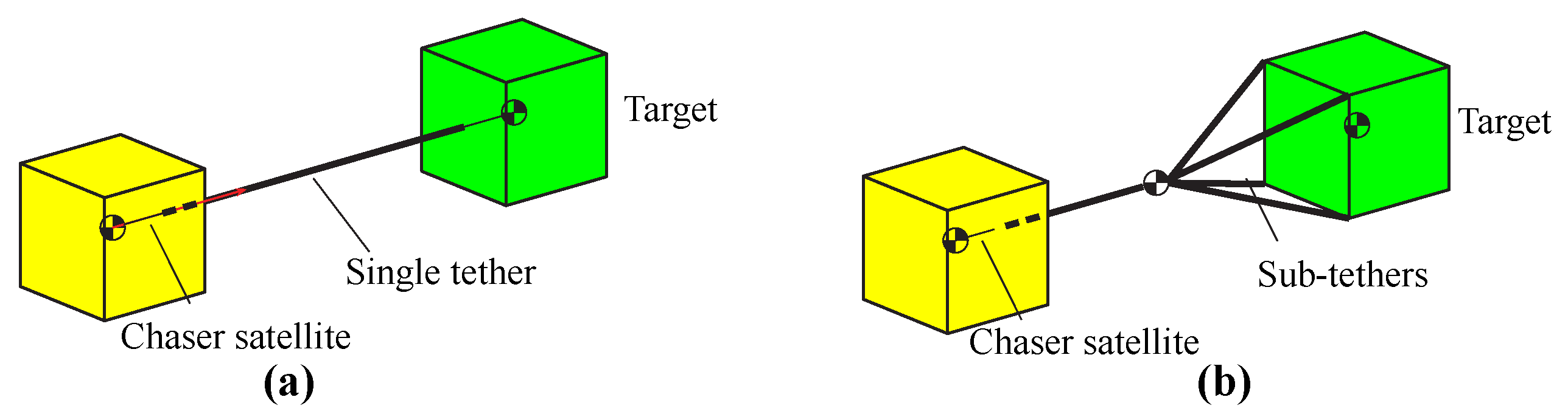
2.1. Configuration of Tethered System

As introduced in Section 1, to remove a space debris object from orbit, a chaser satellite slides close to a target, captures it and deorbits together with it or sends it to a graveyard orbit. The tethered combined system consists of the chaser satellite, the target and the tether connecting them. Hovell and Ulrich have proposed two configurations for the combined system as shown in Figure 3; one is the single tether configuration and the other is the sub-tether configuration in which the tether attached to the service satellite branches into four smaller tethers that are attached to the target at various locations [27]. The single tether configuration as shown in Figure 3a is more suitable for describing the harpoon system and the tether–gripper system. However, it is better to use the sub-tether configuration to model the simplified net system since it can better describe the interaction between the net and the target, even though no contact effect between the net and target is taken into consideration (see Figure 3b). It is noteworthy that the only difference between these two configurations is regarding the existence of sub-tethers. Dynamic analysis of these configurations in a planar environment has been performed and experimentally validated [28]. In this paper, we provide multiple modeling methods for the configurations and investigate their dynamics in a 3D environment.

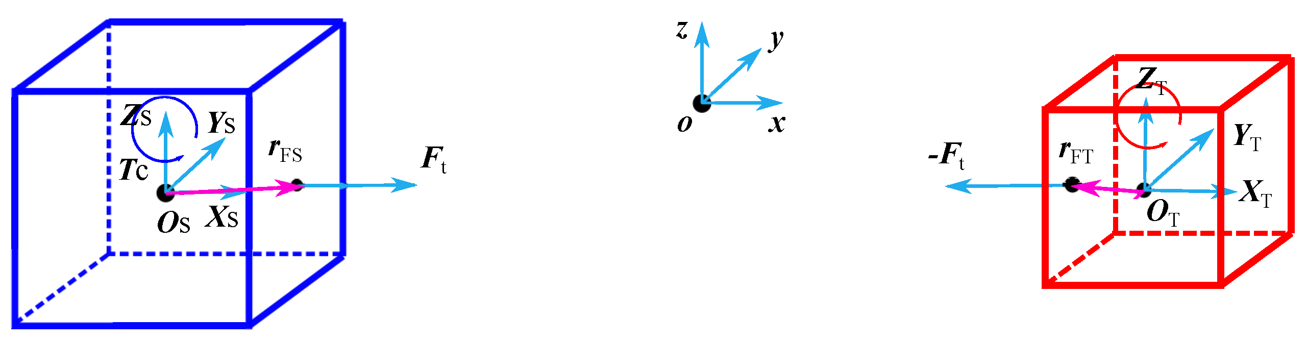
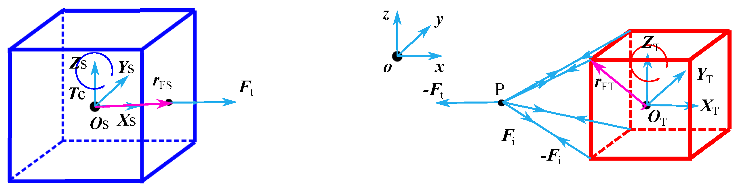
2.2. Modified Dumbbell Model

2.2.1. Single Tether Configuration

The traditional dumbbell model was used for modeling the tethered satellite system, in which two satellites are simplified as tip masses connected by a rigid rod. Misra et al. have used this dumbbell model to analyze the motion of a tethered system in the stationkeeping phase [29]. However, the tether is assumed to be rigid and its length is constant, thus not accurately describing the physical properties of a tether. Figure 4 displays the concept of the proposed modified dumbbell model for the single tether configuration. In the proposed model, o x y z represents the inertial frame, O S X S Y S Z S and O T X T Y T Z T represent the body frame of the satellite and the target, respectively. Points S and T are two ends of the connecting positions of the tether on each object, and r F S and r F T are two position vectors resolved in their individual body frame. The constraint between the satellite and the target is assumed as a force constraint rather than a geometrical one. This force F t is defined as a function of the distance between two objects and written as
F t = ( E A ( L L 0 ) L + c L ˙ ) i L > = L 0 0 L < L 0
where E is the Young’s Modulus of the tether, A is the cross-section of the tether, L is the current distance between two connecting points, L 0 is the initial length of the tether, and i indicates the direction of the force which should be pointing from one connecting point to the other, c is the damping coefficient. The satellite and target are regarded as two rigid bodies instead of end masses. Their governing equations are written as
m k a k = F k ± F t ,
J k ω ˙ k + ω k × J k ω k = T k ,
where k = S , T , and S and T represent the satellite and target, respectively. In Equation (3), m k , J k represent the mass and moment of inertia, a k and ω k represent the linear acceleration and angular velocity of the rigid bodies, F k represents the external force such as microgravity and aerodynamic drag ect. and T k represents the external torque.

2.2.2. Sub-Tether Configuration

The above section provides the modified dumbbell model for the single tether configuration after capturing a space debris object. This model can be easily extended to a sub-tether configuration as shown in Figure 3b only by adding four sub-tethers in the model. The concept of the modified dumbbell model for the sub-tether configuration is shown in Figure 5, where a mass point has to be added at the intersection point P and its governing equation is
m j a j = F i F t ,
where m j is the lumped mass of the main tether and sub-tethers, a j the acceleration of the mass point and F i ( i = 1 , 2 , 3 , 4 ) is the tension forces in sub-tethers, respectively. The tension force F i can be obtained similarly via Equation (1) by changing parameters to those of the sub-tethers.

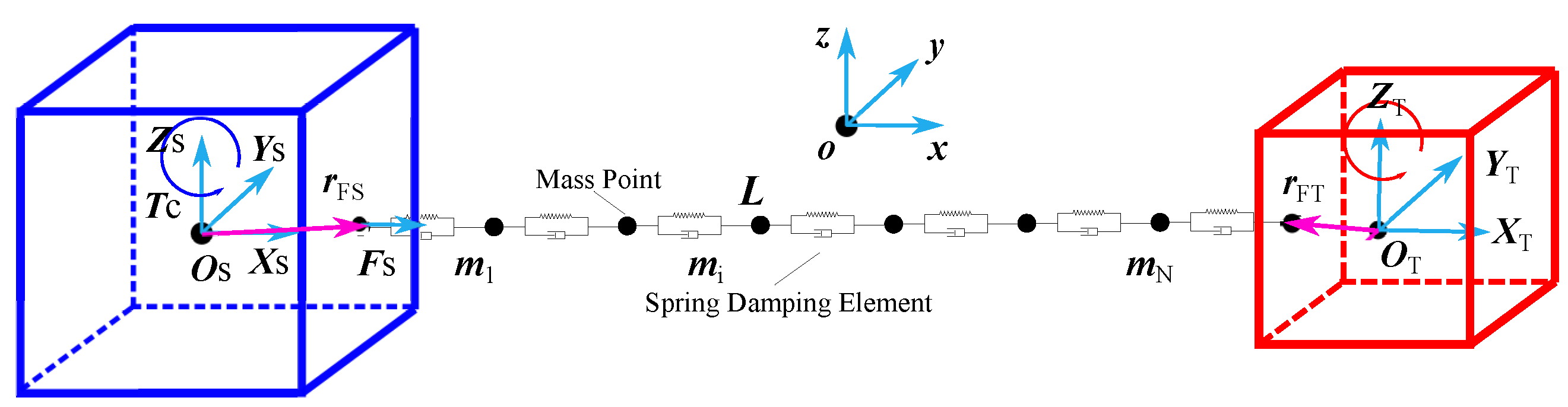
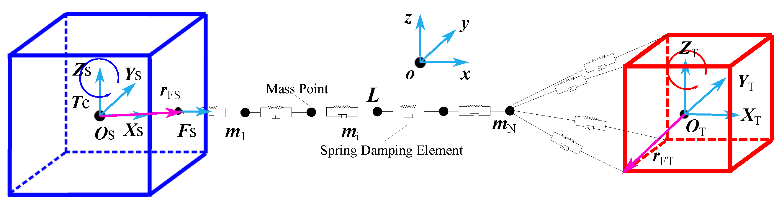
2.3. Lumped-Mass Model

2.3.1. Single Tether Configuration

The lumped-mass model has been widely used in the modeling of a net and/or a tether, and it was also called the mass–spring model. The basic idea of this model is to discrete the tether as a series of mass points connected by a non-linear spring–damper element. Its concept is shown in Figure 6. The reason that the spring–damper element is non-linear is due to the spring’s capability for standing tension but not compression. This property allows the spring to better describe the nature of a tether. The lumped-mass model has been widely discussed in references [9,10,16], and the tension force F i j between nodes i and j is given as
F i j = ( E A l 0 ( r i j l 0 ) 2 ξ m i k r ˙ i j ) r ^ i j r i j > l 0 , 0 r i j l 0 ,
In this equation, r i j and r ˙ i j are the distance and relative velocity between the i-th and j-th node. Furthermore, r ^ i j represents the unit direction vector pointing from the i-th node to the j-th node. l 0 is the initial unstretched mesh length, ξ is its damping ratio, and m i is the mass of the i-th node. The model of two rigid bodies is the same as the modified dumbbell model in Equation (3).

2.3.2. Sub-Tether Configuration
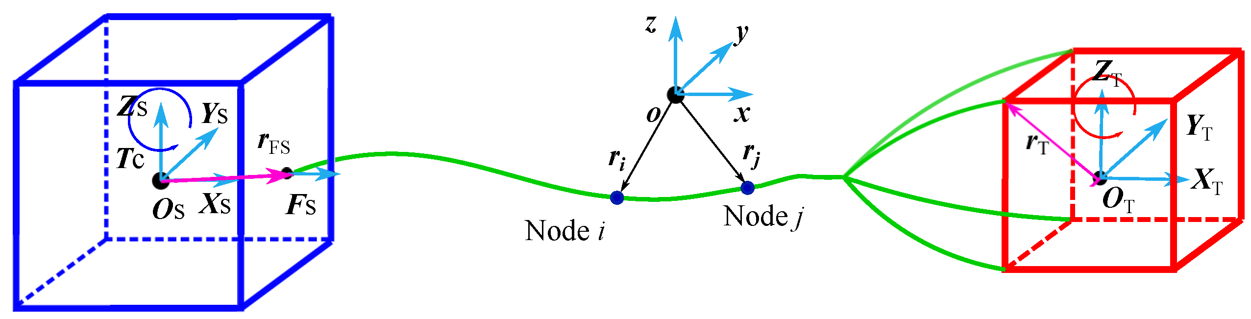
Similar to the modified dumbbell model for the sub-tether configuration, the lumped mass model can also be extended by adding four sub-tethers in the model as shown in Figure 7. Their dynamic equations can be obtained using the same method and are therefore not repeated here again.

2.4. ANCF Model

2.4.1. Single Tether Configuration

Absolute Nodal Coordinates Formulation (ANCF) was originally proposed by Shabana and is utilized in solving large displacement and deformation problems [30]. In ANCF, absolute positions and the gradients of the positions act as the element nodal coordinates to describe the configuration of a flexible system. In contrast, infinitesimal or finite rotations are used as nodal coordinates in the classical finite element method that limits its use to problems with small deformations and rotations. Moreover, the mass matrix in ANCF is constant and no centrifugal and Coriolis forces are involved in the derivation of dynamic equations.
To establish an ANCF model for a combined tethered system, the dynamic models of two rigid bodies are the same as the other two models mentioned in Equation (3); the model of the tether is however built by the ANCF cable element. The concept of the ANCF model for the tethered system is shown in Figure 8.
One cable element contains two end nodes and the arbitrary position in a cable element can be expressed as,
r = S e
where S = [ S 1 I , S 2 I , S 3 I , S 4 I ] is the global shape function, I is a 3×3 identity matrix, e = [ e 1 , e 2 ] T is the absolute nodal coordinates at two ends of the cable element. It is certain that
e i = [ r i , r i x ] ( i = 1 , 2 ) ;
where r i is the global displacement and r i x = r i x is the global slope of the element. The shape function S i is defined as
S 1 = 1 3 ξ 2 + 2 ξ 3 , S 2 = l 0 ( ξ 2 ξ 2 + ξ 3 ) , S 3 = 3 ξ 2 2 ξ 3 , S 4 = l 0 ( ξ 2 + ξ 3 ) ,
where ξ = x / l 0 , and x is the coordinate of arbitrary point on the element.
The constant mass matrix M i can be derived by evaluating the kinetic energy expression which is
T i = 1 2 V ρ r ˙ i T r ˙ i V = 1 2 e ˙ i T M i e ˙ i
where ρ is the density of the element material and r ˙ i is the velocity of the i-th element. The constant mass matrix M i is consequently obtained as
M i = V ρ S T S d V .
The elastic forces of a cable element can be derived from the elastic energy, and that of a deformed cable element contains two parts: the strain energy due to longitudinal deformation and the strain energy due to bending. The strain energy due to longitudinal deformation and bending is, respectively, expressed as
U l a = 1 2 0 l 0 E A ε l 2 d x , U l b = 1 2 0 l 0 E I κ l 2 d κ ,
where ε l can be expressed based on Cauchy–Green longitudinal strain as
ε l = 1 2 ( r T r 1 ) .
and the curvature κ of the cable centerline is given by the formula derived from the Seret–Frenet frame as
κ = | r x × r x x | | r x | 3 .
Using the expression of the strain energy, one obtains the vector of elastic forces
Q e = U e T = K e
and K is the nonlinear stiffness matrix of the element. In order to minimize the number of mathematical operations in the computer implementation, Gaussian quadrature was used for the integration of the non-rational strain energy expressions to approximate the elastic forces. The expressions of the elastic forces in ANCF are non-linear and coordinate- or time-dependent. Several simplified models of elastic forces for the beam element have been derived by Berzeri and Shabana [31].
In the tethered system, two ends of the tether are constrained with two rigid bodies, respectively. This makes the system a coupled rigid–flexible multibody system. Using the principle of virtual power and introducing the Lagrange multipliers, one can derive the system equations of motion for the tethered system as
M e 0 0 M r Φ q T Φ q 0 e ¨ q ¨ r λ = Q e Q r γ
where M e and M r are the constant ANCF mass matrix and rigid bodies mass matrix, respectively; Q e is the generalized elastic force associated with absolute nodal coordinates e , and Q r is the external force applied on the rigid bodies which is governed by its coordinates q r ; here, λ represents the Lagrange multiplier; Φ q is the Jacobin matrix of the constraint equations Φ (Equation (16)); γ is obtained by differentiating the constraint equations twice with respect to time. Based on the configuration of the tethered system in Figure 8, two ends of the tether are constraint with two rigid bodies by sphere joints and the constraint equations of the system is expressed as
Φ = r c + A u Se = 0 ,
where r c is the mass center of a rigid body; u is the vector pointing to the connecting position in the body frame and A represents the rotation matrix with respect to the inertial frame. Differentiating the constraint equations once with respect to time will obtain
Φ ˙ = r c ˙ + A ˙ u S e ˙ = 0 ,
in which the derivative of the rotation matrix is complicated to compute. With the help of the expression of the angular velocity
ω ˜ = A ˙ A T ,
where ( ) ˜ represents the anti-symmetric matrix of the vector ( ) , one can easily simplify the Equation (17) as
Φ ˙ = r c ˙ + ω ˜ A u S e ˙ = 0 .
Differentiating the above equation once more with respect to time will produce
Φ ¨ = r c ¨ + ω ˙ ˜ A u ω ˜ ω ˜ A u S e ¨ = 0 ,
from where the Jacobin matrix Φ q and the term γ can be obtained.

2.4.2. Sub-Tether Configuration

Compared with the single tether configuration under ANCF model, the sub-tether configuration shown in Figure 9 contains more constraint equations. They not only include the constraints of the connecting point with the rigid body, but also include the constraint at the intersection point, whose constraint equation is
e s i e e = 0 ,
in which e s i is the vector of absolute nodal coordinates of the start of sub-tether i (i = 1,2,3,4), and e e is the vector of the end of the main tether. The structure of system equations and derivations makes no difference with the single tether configuration.

3. Modal Analysis of Tethered System

3.1. Analytical Results

Section 2 describes three dynamic modeling methods for a tethered post-capture system, and two of them do not consider the bending stiffness of the main tether. Therefore, this section only discuss the axial vibration of the main tether for modal analysis. Since a tether is not able to withstand compression, the tether becomes slack when the distance between two end bodies is smaller than the original length of the tether. To establish the theoretical model of the tether for modal analysis and to determine the optimal number of segments, the tether is divided in the simulation, the main tether is assumed as an elastic rod, and two end bodies are assumed as two mass points for analysis in this section. It is easy to establish the equation of equilibrium for a elastic rod as
E 2 u ( x , t ) x 2 = ρ 2 u ( x , t ) t 2 ,
where E, ρ are the Young’s modulus and density of the main tether. Here, u ( x , t ) is the solution of displacement along the tether, and it is feasible to assume its form as follows
u ( x , t ) = ϕ ( t ) U ( x ) = [ a sin ( ω t ) + b cos ( ω t ) ] [ c sin ( λ x ) + d cos ( λ x ) ] ,
where a , b , c , d are underdetermined coefficients, λ = ω ρ / E and ω is its natural frequency. Underdetermined coefficients can be obtained by substitution of boundary conditions into Equation (23). It is easy to find the analytical solution of natural frequencies for an elastic rod or string with free–free boundary conditions in any structural dynamics textbook, which is
ω n = n π l E ρ , n = 1 , 2 , ,
where l is the length of the elastic rod or string.
However, a tethered post-capture system contains not only the main tether but also two end-lumped masses. The boundary conditions for the system therefore become
E A u ( 0 , t ) x m S 2 u ( 0 , t ) t 2 = 0 , E A u ( L , t ) x m T 2 u ( L , t ) t 2 = 0 ,
where m S and m T represent the mass of the satellite on left and the target on right in Figure 4, respectively. Substitution of Equation (25) into Equation (23) is able to obtain the characteristic equation of the tethered system as
tan ( λ l ) = E A λ ( m S + m T ) m S m T ω 2 E ρ A 2 .
Therefore, the corresponding natural frequencies of a tethered system can be obtained by solving Equation (26). Since the radius of the main tether is usually small, the second term in the denominator in Equation (26) is negligible, and it can be further simplified as
tan ( ω l ρ / E ) = E ρ A ( m S + m T ) m S m T ω .

3.2. Modified Dumbbell Model

Based on the derivation of the modified dumbbell model in Section 2.2, it is straightforward to write the equations of motion of an undamped tethered system in matrix form as
M u ¨ + K u = 0 .
where M and K are the mass and stiffness matrix of the tethered system, u is the displacement vector of two end masses. Their explicit forms are
M = m S 0 0 m T , K = k k k k , u = u S u T ,
where k = E A / L is the stiffness of the tether, u S and u T are the displacement of the satellite and target, respectively.
Then the frequencies and mode shapes of the tethered system can be obtained by solving the eigenvalue problem
( K ω 2 M ) u = 0 .
Simply changing the mass of the satellite and target to half the mass of the tether in the mass matrix is able to achieve the frequencies and mode shapes of the tether without tip masses.

3.3. Lumped-Mass Model

The equations of motion of the tethered system under the lumped-mass model have the same form with that of the dumbbell model as shown in Equation (28). The mass matrix and stiffness are different as follows
M = m S m i m i m T , K = k k 0 0 0 k 2 k k 0 0 0 0 0 0 k 2 k k 0 0 0 k k ,
where m i = m t / N is the distributed mass along the tether, m t the mass of the tether, N the number of the mass points, k = N E A / L the stiffness of each segment. It results in the same eigenvalue problem as Equation (30). For there to be a nontrivial solution of Equation (30), the determinant of the matrix K ω 2 M should be zero. Solving the characteristic equation obtains the natural frequencies of the system. Changing the mass m S and m T to m i in mass matrix is also able to achieve the frequencies of the tether without tip masses.

3.4. ANCF Model

In Section 2.4, the constant mass matrix M i in the ANCF model has been derived. The stiffness matrix of a tether can be obtained by taking the derivative of elastic force with respect to the generalized coordinates e , or taking the derivative of strain energy with respect to e twice. Since we only consider the axial vibration of the tether, we use the strain energy due to longitudinal deformation only. The stiffness matrix is therefore
K i = 2 U l a e 2 .
Performing the derivative, we can obtain
K i = 0 l E A ε l e ε l e d x + 0 l E A ε l 2 ε l e 2 d x .
It is seen from the above equation that the stiffness matrix is dependent on the current configuration of the system. Since calculating the natural frequency only requires the stiffness matrix at an initial configuration, and we assume there is no initial stress in the system, i.e., ε l is zero in the beginning, the second term of the stiffness matrix in Equation (33) is therefore zero. Only the first term is left. The expression of ε l is already shown in Equation (12). Taking the derivative of ε l with respect to e yields
ε l e = S x T S x e = S a e .
where S x is the first derivative of shape function S with respect to position coordinates x, and S a = S x T S x for short. Note that
S a = S x T S x = 1 l 0 2 S ξ T S ξ = 1 l 0 2 S b .
where S b = S ξ T S ξ for short, and S ξ is the first derivative of shape function S with respect to natural coordinates ξ .
Therefore, the initial stiffness matrix becomes
K i = 0 l E A ε l e ε l e d x = 0 l E A ( S a e ) ( S a e ) d x = E A l 0 3 0 1 ( S b e ) ( S b e ) d ξ .
The above achieved mass matrix and stiffness matrix are for one element. Assemble them to obtain the system mass matrix M and stiffness matrix K . Use Equation (30) to solve the eigenvalue problem and achieve the natural frequency and mode shapes for the main tether without tip masses. It is noteworthy that the mass matrix need to be modified if a tethered system is considered. The rigid tip mass should be added and the new mass matrix becomes
M n = M + M r .

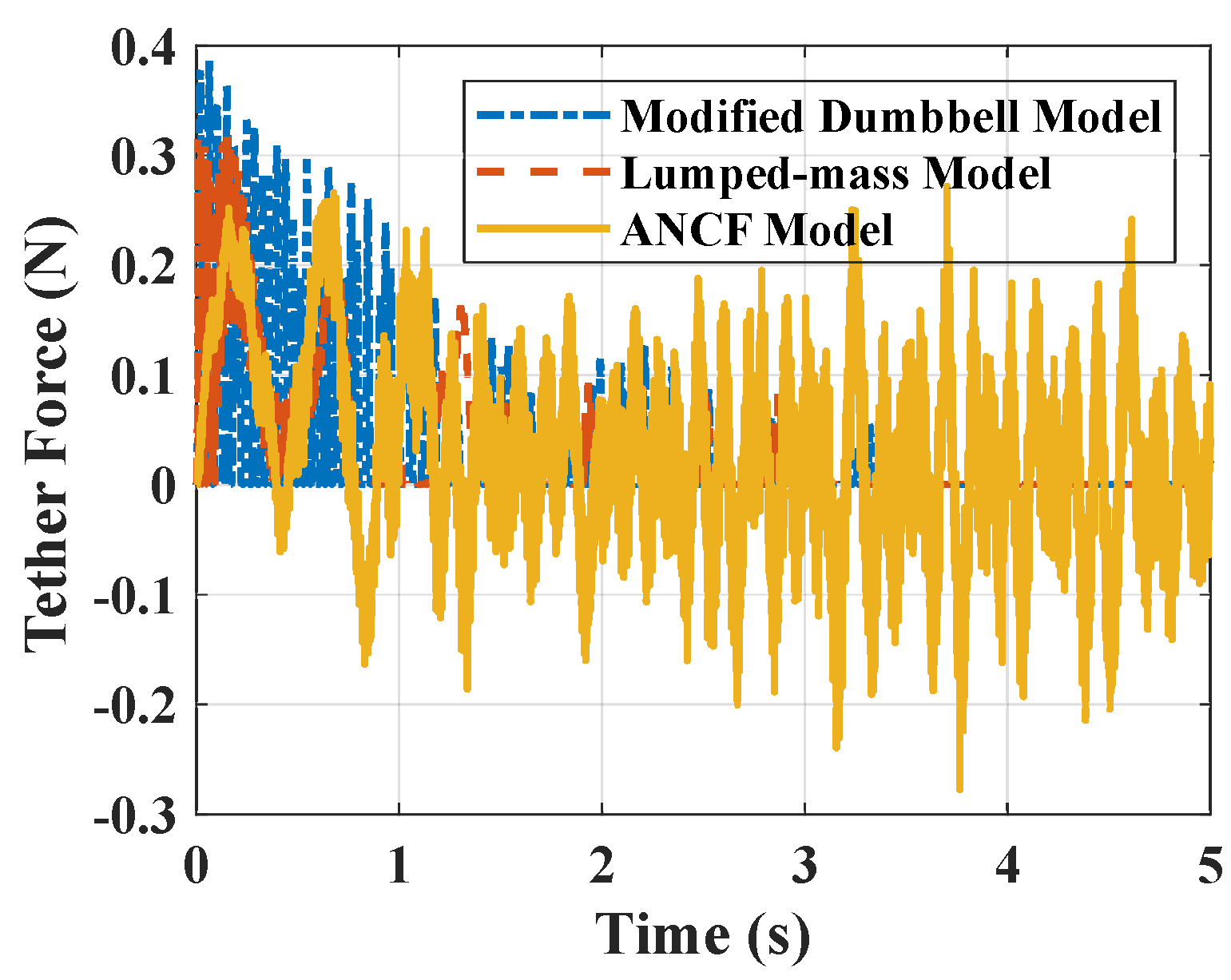
4. Comparison of Three Models

To systematically compare three modeling methods for tethered system after capturing a space debris object provided in Section 2, simulations of both the single tether configuration and the sub-tether configuration are performed based on the above three models in this section. Six groups of simulations in total, two configurations under three models, respectively, are run and the results are compared. Moreover, natural frequencies are calculated based on three models and the results are compared with the analytical solution. Moreover, the influence of the initial conditions of the tethered system is also discussed.

4.1. Single Tether Configuration

For the harpoon method and the tether–gripper method, the combined system can be simplified as two rigid bodies connected by a flexible tether as shown in Figure 3a. The target is assumed as a Cubesat weights 3.5 kg, to be captured by a 10 kg chaser Cubesat equiped with a harpoon or gripper. As most of the space debris is tumbling due to its residual momentum, we set the initial angular velocity of the target as 0.3 rad/s rotating about its axis with the largest moment of inertia. Other simulation parameters are summarized in Table 1.
Simulations of the tethered system with the parameters in Table 1 under three models were performed. Screenshots of the animations are listed and compared in Table 2. It can be seen that their configurations at the same moments under three models are close to each other. Figure 10 shows the position trajectory of the mass center of the target along the x direction. It can be seen that the curves overlap each other, indicating that the three models are all able to describe the motion of system correctly. The change of the angular velocity of the target is shown in Figure 11 and it indicates that the tether force applies on the target and generates a torque on the target, thus detumbling the target. Its angular velocity is decreased from 0.3 rad/s to around 0.21 rad/s in 5 s, and all the three models present quite close results. In this respect, it is implied that a tethered system is not only able to capture a target but also able to detumble the target simultaneously. As shown in Figure 12, the tether force in the modified dumbbell model and the lumped-mass model is always positive. This is because that the tether in those two models is not able to withstand compression but only tension. In contrast, the tether in ANCF model can withstand both. In addition, in the first two models, it is also seen that the force is not always applied on the tether. It is zero when the tether is not at tension.

4.2. Sub-Tether Configuration

For the net capturing method, the combined system model can be simplified as two rigid bodies connected by a main flexible tether and four sub-tethers as shown in Figure 3b. When a net finishes capturing a target, not all cables of the net are at tension. Therefore, it is reasonable to simplify the net as four sub-tethers connecting to the target, which is a typical configuration proposed by Hovell and Ulrich for the post-capture system by a net [28]. Here, we use this sub-tether configuration in the simulation and the contact between the net and the target is not taken into consideration. Table 3 lists the screenshots of animations of three models. It is not surprising to notice that those configurations at the same moments have good agreements. Figure 13, Figure 14 and Figure 15 display the position, angular velocity of the target and the tether force with respect to time, respectively. Similar conclusions can be drawn to the simulation of the single tether system except for the complicated situation in the sub-tether configuration. Moreover, the angular velocity of the target is decreased 20% more than that of a single tether system in 5 s, which implies that the sub-tether configuration has more detumbling efficiency than that of the single tether configuration. The reason of why the simulation is run up to 5 s is because the tumbling target will entangle with the main tether if no control is performed after 5 s. In that case, the contact detection algorithm and contact dynamics have to be considered, which is not the focus of this paper.

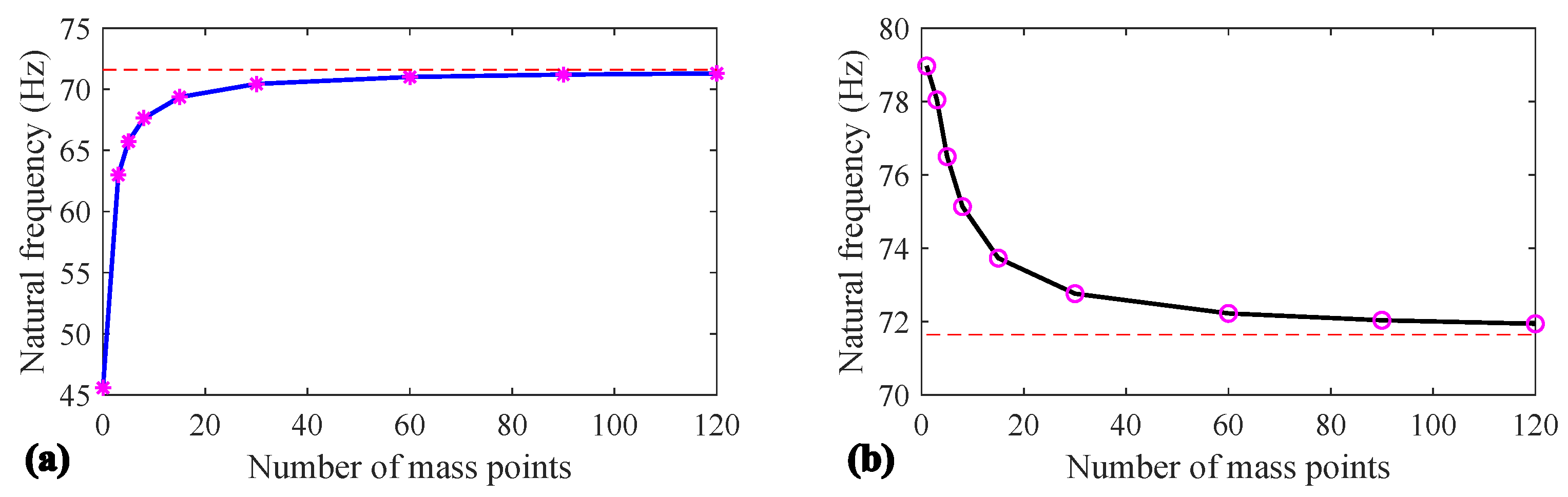
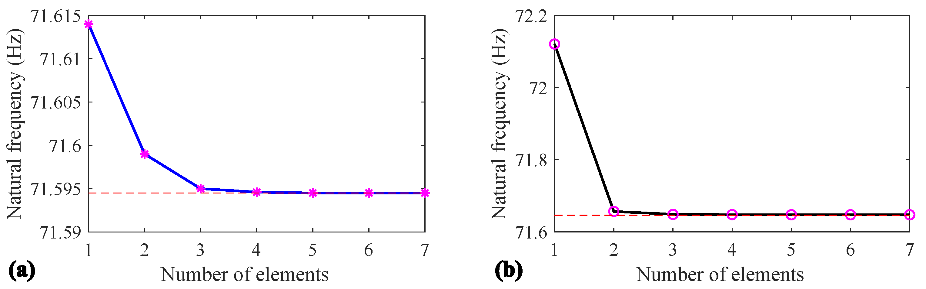
4.3. Comparison of Natural Frequency

To further compare three models from the viewpoint of vibration, the natural frequencies of the main tether and the tethered system based on three models are calculated and compared with the analytical results introduced in Section 3. The parameters of the system are the same as shown in Table 1. First five orders of natural frequencies of the main tether and the tethered system are shown in Table 4 and Table 5, respectively. Since the modified dumbbell model only has two degrees of freedom in 2D space and one of the mode is the rigid motion, it has only the first order of natural frequency and that of the main tether is far from the analytical result. Natural frequencies of the main tether based on the lumped-mass model are close to the analytical. However, the results come from the discrete model with 100 mass points along a 2.25-m elastic tether. For comparison, the ANCF model only requires seven elements to receive even closer results. When it comes to the tethered system, two end masses are attached at both ends and the first order of natural frequency drops down dramatically. It is also interesting to see that the modified dumbbell model is able to capture that mode accurately. The lumped-mass model with 10 discrete mass points can already obtain a quite close match, let alone the 7-element ANCF model. This is because the mass of the tether is much smaller than that of two end masses; therefore, the end masses dominate the natural frequency of the system.
It can be seen that more discrete mass points and elements in the model will lead to a more accurate result based on the above discussion. However, more discrete elements will definitely increase the computational time. In order to choose the optimal number of points into which the tether is divided to maintain the efficiency and adequacy of the simulation, convergence study for both the lumped mass model and the ANCF model is carried out. Figure 16 and Figure 17 show the convergence of natural frequencies to the analytical results with respect to the increasing elements under two models. On one hand, this analysis indicates both models are able to describe the dynamics of a tether and tethered system accurately, and they are cross-verified. On the other hand, this analysis provides the reader a guideline of how to choose a proper number of elements from a viewpoint of vibration.

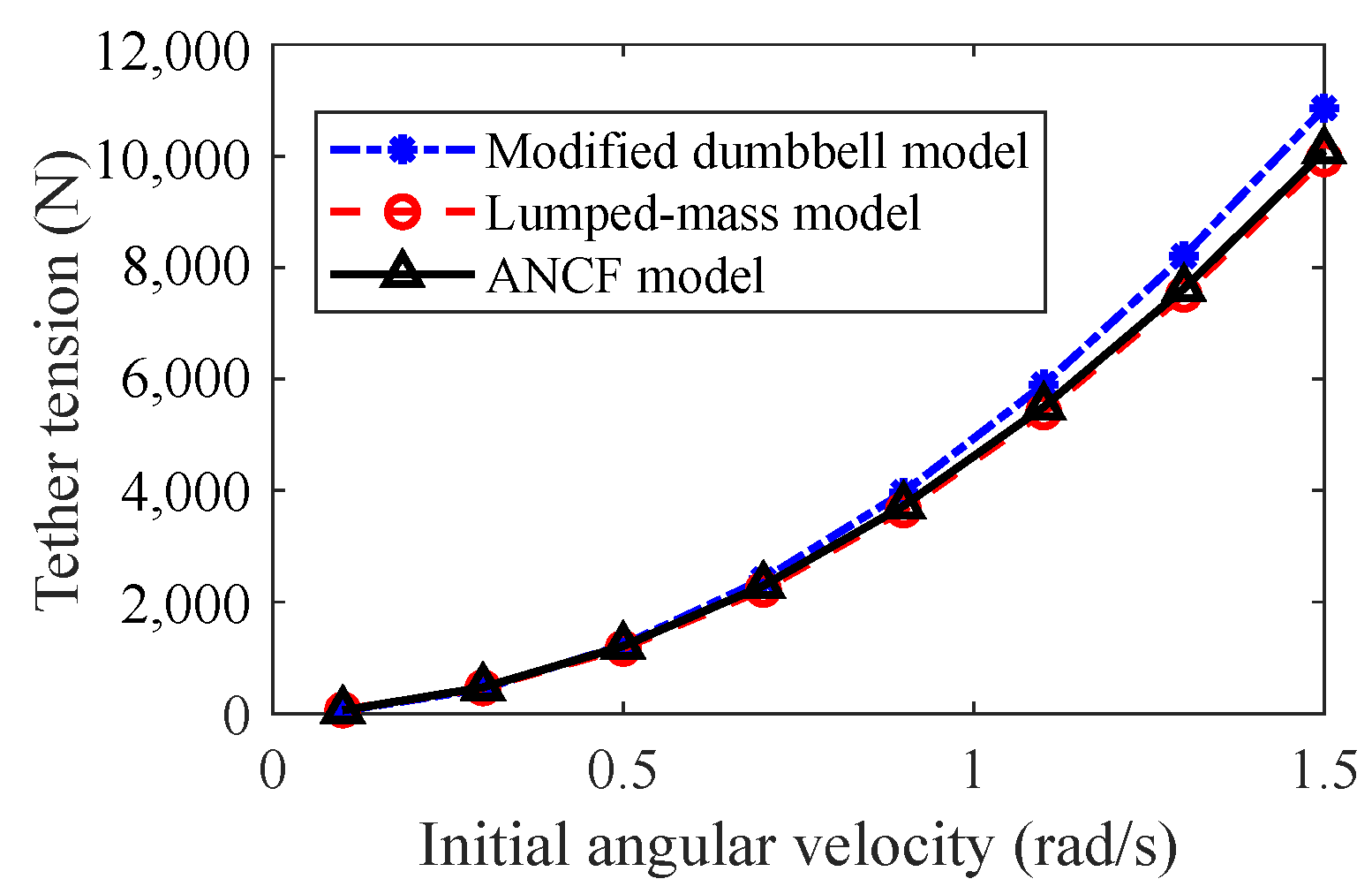
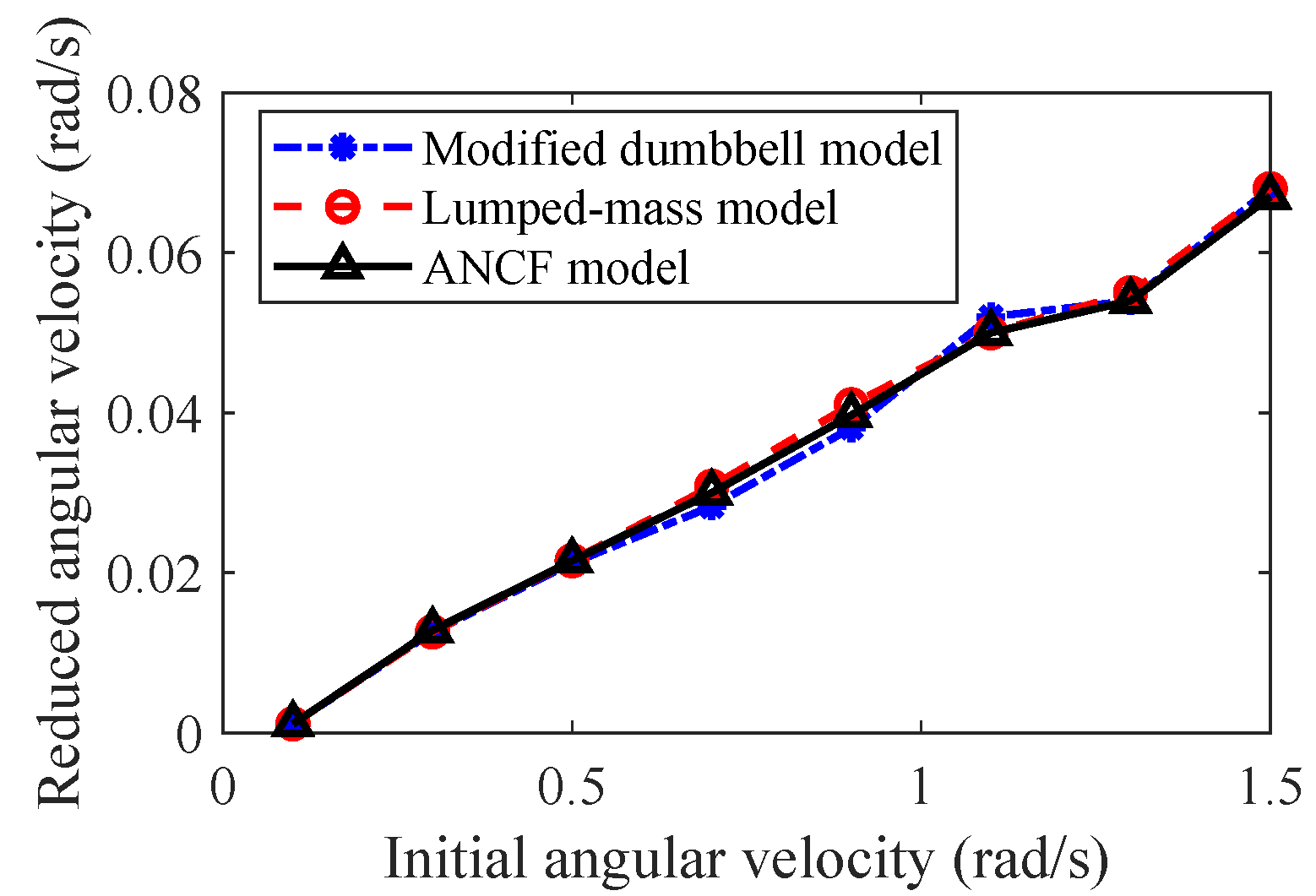
4.4. Influence by Initial Condition

Section 4.1 and Section 4.2 introduced the cross-verification of the three presented models when dealing with a small target. However, the most threatening and urgent targets to be removed are usually massive ones. This section discusses a removal of an 8-ton target by a Microsat weighing 500 kg. Since a rotating massive target can cause a huge force in the tether, thus pulling the satellite, the faster it rotates, the larger the force will be; Kevlar is strong enough to be selected as the material of the main tether. To investigate how this impact force changes with respect to the initial angular velocity of a massive target, simulations based on those three models were performed, and the simulation parameters are summarized in Table 6.
Figure 18 describes the changing of the impact force on the satellite when the target rotates based on three models. It can be seen that the impact force is non-linearly changing with respect to the target’s initial angular velocity. Moreover, three models present the same trend and relatively closer values of the tether tension force, that of lumped-mass model and ANCF model almost overlap each other. Since the tether tension force will generate an inverse torque on the target thus detumbling it, the reduced values of target’s angular velocity is shown in Figure 19, which also have good agreements among three models.

5. Conclusions

This paper compares three models of describing a tethered post-capture system for space debris removal, namely the modified dumbbell model, lumped-mass model and the ANCF model. Three models have been established in detail and modal analysis of the tethered system was performed. Comparison among three models was deeply made via numerical simulations. Simulations of different case studies have shown good agreements among models. By running simulations of both the single tether system and the sub-tether system, it concludes that the tethered-system is able to capture a target and de-tumble a target simultaneously, and the sub-tether configuration is more efficient in detumbling a target than the single tether configuration. Comparison of natural frequencies of a tethered system provides the cross-verification from the viewpoint of vibration, and the convergence study offers a guideline to determine the number of elements in the lumped-mass model or ANCF model. In addition, it was found that the impact force on the satellite is non-linearly dependent on the target’s initial angular velocity. Based on those comparisons, three models are all able to predict the motion of a tethered system accurately. However, the modified dumbbell model is recommended to model a tether system as a first guess due to its simplicity. Both the lumped-mass model and the ANCF model are able to describe the flexibility and longitudinal vibration of the main tether, but the ANCF model requires less elements to capture the dynamics of it. Future study will focus on the detumbling control and the orbital effect influence of the tethered system during de-orbiting based on those models.

Author Contributions

Conceptualization, M.S. and L.S.; methodology, M.S.; software, M.S.; validation, M.S. and L.S.; formal analysis, M.S.; investigation, M.S.; resources, L.S.; data curation, L.S.; writing—original draft preparation, M.S.; writing—review and editing, L.S.; visualization, L.S.; supervision, L.S.; project administration, M.S.; funding acquisition, M.S. All authors have read and agreed to the published version of the manuscript.

Funding

This research was funded by National Natural Science Foundation of China, grant number 12102034 and Beijing Institute of Technology Research Fund Program for Young Scholars.

Institutional Review Board Statement

Not applicable.

Informed Consent Statement

Not applicable.

Conflicts of Interest

The authors declare no conflict of interest.

References

  1. NASA Orbital Debris Program Office. Orbital Debris Quaterly News; National Aeronautics and Space Administration: Washington, DC, USA, 2021; Volume 25, pp. 1–12. [Google Scholar]
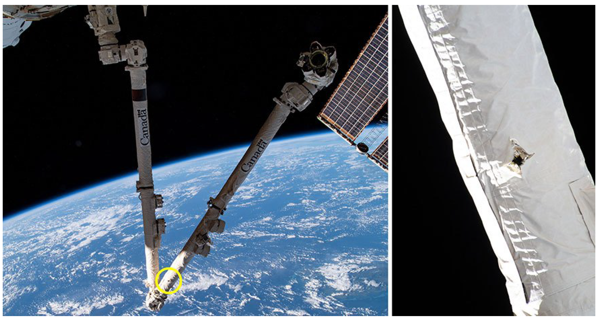
  2. GlobalNews. Damage on Canadarm. 2021. Available online: https://globalnews.ca/news/7913922/canadarm2-damaged-international-space-station-junk/ (accessed on 7 June 2021).
  3. Shan, M.; Guo, J.; Gill, E. Review and comparison of active space debris capturing and removal methods. Prog. Aerosp. Sci. 2016, 80, 18–32. [Google Scholar] [CrossRef]
  4. Reed, J.; Barraclough, S. Development of harpoon system for capturing space debris. In Proceedings of the 6th European Conference on Space Debris, Darmstadt, Germany, 22–25 April 2013; Volume 723, p. 174. [Google Scholar]
  5. Bischof, B. ROGER-Robotic geostationary orbit restorer. In Proceedings of the 54th International Astronautical Congress of the International Astronautical Federation, Bremen, Germany, 29 September–3 October 2003. [Google Scholar]
  6. Tamaki, Y.; Tanaka, H. Penetration Characteristics of Metal Harpoons with Various Tip Shapes for Capturing Space Debris. In Proceedings of the 8th European Conference on Space Debris, Darmstadt, Germany, 20–23 April 2021. [Google Scholar]
  7. Sizov, D.A.; Aslanov, V.S. Space Debris Removal with Harpoon Assistance: Choice of Parameters and Optimization. J. Guid. Control. Dyn. 2020, 44, 767–778. [Google Scholar] [CrossRef]
  8. Cleary, S.; O’Connor, W.J. Control of space debris using an elastic tether and wave-based control. J. Guid. Control. Dyn. 2016, 39, 1392–1406. [Google Scholar] [CrossRef]
  9. Shan, M.; Guo, J.; Gill, E. Deployment Dynamics of Tethered-Net for Space Debris Removal. Acta Astronaut. 2017, 132, 293–302. [Google Scholar] [CrossRef]
  10. Botta, E.M.; Sharf, I.; Misra, A.K.; Teichmann, M. On the simulation of tether-nets for space debris capture with Vortex Dynamics. Acta Astronaut. 2016, 123, 91–102. [Google Scholar] [CrossRef]
  11. Benvenuto, R.; Salvi, S.; Lavagna, M. Dynamics analysis and GNC design of flexible systems for space debris active removal. Acta Astronaut. 2015, 110, 247–265. [Google Scholar] [CrossRef]
  12. Golebiowski, W.; Michalczyk, R.; Dyrek, M.; Battista, U.; Wormnes, K. Validated simulator for space debris removal with nets and other flexible tethers applications. Acta Astronaut. 2016, 129, 229–240. [Google Scholar] [CrossRef]
  13. Medina, A.; Cercós, L.; Stefanescu, R.M.; Benvenuto, R.; Pesce, V.; Marcon, M.; Lavagna, M.; González, I.; López, N.R.; Wormnes, K. Validation results of satellite mock-up capturing experiment using nets. Acta Astronaut. 2017, 134, 314–332. [Google Scholar] [CrossRef]
  14. Shan, M.; Guo, J.; Gill, E.; Golebiowski, W. Validation of Space Net Deployment Modeling Methods Using Parabolic Flight Experiment. J. Guid. Control. Dyn. 2017, 40, 3319–3327. [Google Scholar] [CrossRef]
  15. Aglietti, G.; Taylor, B.; Fellowes, S.; Ainley, S.; Tye, D.; Cox, C.; Zarkesh, A.; Mafficini, A.; Vinkoff, N.; Bashford, K.; et al. RemoveDEBRIS: An in-orbit demonstration of technologies for the removal of space debris. Aeronaut. J. 2020, 124, 1–23. [Google Scholar] [CrossRef]
  16. Benvenuto, R.; Lavagna, M.; Salvi, S. Multibody dynamics driving GNC and system design in tethered nets for active debris removal. Adv. Space Res. 2016, 58, 45–63. [Google Scholar] [CrossRef]
  17. Botta, E.M.; Sharf, I.; Misra, A.K. Contact Dynamics Modeling and Simulation of Tether Nets for Space-Debris Capture. J. Guid. Control. Dyn. 2016, 40, 110–123. [Google Scholar] [CrossRef]
  18. Zhang, F.; Huang, P. Releasing dynamics and stability control of maneuverable tethered space net. IEEE/ASME Trans. Mechatronics 2016, 22, 983–993. [Google Scholar] [CrossRef]
  19. Zhang, F.; Huang, P.; Meng, Z.; Zhang, Y.; Liu, Z. Dynamics analysis and controller design for maneuverable tethered space net robot. J. Guid. Control. Dyn. 2017, 40, 2828–2843. [Google Scholar] [CrossRef]
  20. Huang, P.; Wang, D.; Meng, Z.; Zhang, F.; Guo, J. Adaptive postcapture backstepping control for tumbling tethered space robot–target combination. J. Guid. Control. Dyn. 2015, 39, 150–156. [Google Scholar] [CrossRef]
  21. Pang, Z.; Yu, B.; Jin, D. Chaotic motion analysis of a rigid spacecraft dragging a satellite by an elastic tether. Acta Mech. 2015, 226, 2761–2771. [Google Scholar] [CrossRef]
  22. Forshaw, J.L.; Aglietti, G.S.; Fellowes, S.; Salmon, T.; Retat, I.; Hall, A.; Chabot, T.; Pisseloup, A.; Tye, D.; Bernal, C.; et al. The active space debris removal mission RemoveDebris. Part 1: From concept to launch. Acta Astronaut. 2020, 168, 293–309. [Google Scholar] [CrossRef] [Green Version]
  23. Aglietti, G.S.; Taylor, B.; Fellowes, S.; Salmon, T.; Retat, I.; Hall, A.; Chabot, T.; Pisseloup, A.; Cox, C.; Mafficini, A.; et al. The active space debris removal mission RemoveDebris. Part 2: In orbit operations. Acta Astronaut. 2020, 168, 310–322. [Google Scholar] [CrossRef] [Green Version]
  24. O’Connor, M.; Clearly, S.; Hayden, D. Debris de-tumbling and de-orbiting by elastic tether and wave-based control. In Proceedings of the 6th International Conference on Astrodynamics Tools and Techniques (ICATT), Darmstadt, Germany, 14–17 March 2016. [Google Scholar]
  25. Shan, M.; Shi, L. Post-capture control of a tumbling space debris via tether tension. Acta Astronaut. 2021, 180, 317–327. [Google Scholar] [CrossRef]
  26. Stadnyk, K.; Ulrich, S. Validating the Deployment of a Novel Tether Design for Orbital Debris Removal. J. Spacecr. Rocket. 2020, 57, 1335–1349. [Google Scholar] [CrossRef]
  27. Hovell, K.; Ulrich, S. Attitude stabilization of an uncooperative spacecraft in an orbital environment using visco-elastic tethers. In Proceedings of the AIAA Guidance, Navigation, and Control Conference, San Diego, CA, USA, 4–8 January 2016; p. 0641. [Google Scholar]
  28. Hovell, K.; Ulrich, S. Postcapture dynamics and experimental validation of subtethered space debris. J. Guid. Control. Dyn. 2018, 41, 519–525. [Google Scholar] [CrossRef]
  29. Misra, A.; Nixon, M.; Modi, V. Nonlinear dynamics of two-body tethered satellite systems: Constant length case. J. Astronaut. Sci. 2001, 49, 219–236. [Google Scholar] [CrossRef]
  30. Shabana, A.A. Flexible multibody dynamics: Review of past and recent developments. Multibody Syst. Dyn. 1997, 1, 189–222. [Google Scholar] [CrossRef]
  31. Berzeri, M.; Shabana, A. Development of simple models for the elastic forces in the absolute nodal co-ordinate formulation. J. Sound Vib. 2000, 235, 539–565. [Google Scholar] [CrossRef]
Figure 1. Damage on Canadarm2 [2].
Aerospace 09 00033 g001
Figure 2. Flexible connection capture methods. (a) Harpoon method [4], (b) net method [5], (c) tether–gripper method [5].
Aerospace 09 00033 g002
Figure 3. Configurations of a tethered system [27].
Aerospace 09 00033 g003
Figure 4. Concept of the modified dumbbell model.
Aerospace 09 00033 g004
Figure 5. Concept of the modified dumbbell model for sub-tether configuration.
Aerospace 09 00033 g005
Figure 6. Concept of the lumped-mass model for a single tether configuration.
Aerospace 09 00033 g006
Figure 7. Concept of the lumped-mass model for a sub-tether configuration.
Aerospace 09 00033 g007
Figure 8. Concept of the ANCF model for a single tether configuration.
Aerospace 09 00033 g008
Figure 9. Concept of the ANCF model for sub-tether configuration.
Aerospace 09 00033 g009
Figure 10. Position of the mass center of the target.
Aerospace 09 00033 g010
Figure 11. Angular velocity of the target.
Aerospace 09 00033 g011
Figure 12. Tether force.
Aerospace 09 00033 g012
Figure 13. Position of the mass center of the target.
Aerospace 09 00033 g013
Figure 14. Angular velocity of the target.
Aerospace 09 00033 g014
Figure 15. Tether force.
Aerospace 09 00033 g015
Figure 16. Convergence study of the lumped-mass model. (a) Natural frequency convergence of the main tether; (b) natural frequency convergence of the tethered system.
Aerospace 09 00033 g016
Figure 17. Convergence study of the ANCF model. (a) Natural frequency convergence of the main tether; (b) natural frequency convergence of the tethered system.
Aerospace 09 00033 g017
Figure 18. Impact force on the satellite with respect to the initial angular velocity.
Aerospace 09 00033 g018
Figure 19. Reduced angular velocity with respect to the initial angular velocity.
Aerospace 09 00033 g019
Table 1. Simulation Parameters.
ParameterValue
Service SatelliteMass m S , (kg)10
Dimensions −, (m)0.6 × 0.6 × 0.6
TargetMass m T , (kg)3.5
Dimensions −, (m)0.4 × 0.4 × 0.4
TetherMain tether length L, (m)2.25
Sub-tether length l, (m)0.4123
Tether diameter d, (mm)5
Damping coefficient c, (-)0.1
Young’s modulus E, (Pa) 4.456 × 10 7
Table 2. Simulation Animation Screenshots for Single Tether Configuration.
ModelsScreenshots of Animations
t = 0 s                    t = 2.5 s                    t = 5 s
Modified Dumbbell Model Aerospace 09 00033 i001
Lumped-mass Model Aerospace 09 00033 i002
ANCF Model Aerospace 09 00033 i003
Table 3. Simulation animation screenshots for the sub-tether configuration.
ModelsScreenshots of Animations
t = 0 s                    t = 2.5 s                    t = 5 s
Modified Dumbbell Model Aerospace 09 00033 i004
Lumped-mass Model Aerospace 09 00033 i005
ANCF Model Aerospace 09 00033 i006
Table 4. Natural frequencies of the main tether (Hz).
OrderAnalyticalModified Dumbbell ModelLumped-Mass ModelANCF Model
171.5945.5871.2471.59
2143.19-142.46143.19
3214.78-213.65214.79
4286.38-284.79286.44
5357.97-355.86358.22
Table 5. Natural frequencies of the tethered system (Hz).
OrderAnalyticalModified Dumbbell ModelLumped-Mass ModelANCF Model
11.9471.9491.9481.948
271.646-74.57471.647
3143.216-147.555143.217
4214.802-217.549214.814
5286.392-283.120286.464
Table 6. Simulation parameters.
ParameterValue
Service SatelliteMass m S , (kg)500
Dimensions −, (m)2.5 × 2.5 × 2.5
TargetMass m T , (kg)8000
Dimensions −, (m)5 × 5 × 5
TetherMain tether length L, (m)100
Tether diameter d, (mm)50
Damping coefficient c, (-)0.1
Young’s modulus E, (GPa)131
Publisher’s Note: MDPI stays neutral with regard to jurisdictional claims in published maps and institutional affiliations.

