Article

The Impact of Steady Blowing from the Leading Edge of an Open Cavity Flow

by
Naser Al Haddabi
1,*,
Konstantinos Kontis
2 and
Hossein Zare-Behtash
2
1
Department of Engineering, University of Technology and Applied Sciences, Al Musannah 314, Oman
2
James Watt School of Engineering, University of Glasgow, Glasgow G12 8QQ, UK
*
Author to whom correspondence should be addressed.
Aerospace 2021, 8(9), 255; https://doi.org/10.3390/aerospace8090255
Submission received: 7 July 2021 / Revised: 30 August 2021 / Accepted: 2 September 2021 / Published: 9 September 2021
(This article belongs to the Special Issue Advances in Aerospace Sciences and Technology II)

Abstract

:
Cavity flows occur in a wide range of low-speed applications (Mach number 0.3 ), such as aircraft wheel wells, ground transportation, and pipelines. In the current study, a steady jet is forced from a cavity leading edge at different momentum fluxes (0.11 kg/ms 2 , 0.44 kg/m·s 2 , and 0.96 kg/m·s 2 ). The investigation was performed for an open cavity with length to depth ratio of 4 at the Reynolds number based on a cavity depth of approximately 50,000. Particle image velocimetry, surface oil flow visualisation, constant temperature anemometry, and pressure measurements were performed in this investigation. The aim of the jet blowing is to separate the cavity separated shear layer from the recirculation zone to reduce the cavity return flow, and hence stabilise the cavity separated shear layer. It was found that increasing the jet momentum flux causes an increase in the cavity return flow due to the increase in the thickness of the cavity separated shear layer. The study also found that the jet populates the separated shear layer with a large number of small-scale disturbances. These disturbances increase the broad band level of the pressure power spectra and Reynolds shear stress in the cavity separated shear layer. On the other hand, the jet disturbances make the shedding of the large vortical structures more intermittent.

1. Introduction

Flows over cavities induce strong flow oscillations which can substantially increase noise, drag, and vibration and lead to structural fatigue. Cavity flows impact a wide range of high-speed applications [1,2], as well as low-speed applications. Low-speed applications include aircraft wheel wells, ground transport vehicles, and pipelines [3,4,5].
A typical flow topology within a shallow open cavity at low speeds is illustrated in Figure 1. Due to momentum transfer, the cavity separated shear layer expands as it develops downstream. Eventually, it impinges on the cavity trailing edge. As a result, a portion of the separated shear layer flow deflects back towards the cavity leading edge, forming a large recirculation vortex inside the cavity (main recirculation vortex). Driven by the main recirculation vortex, a weaker recirculation vortex (secondary vortex) is usually formed near the cavity leading edge [6].
The cavity separated shear layer is highly unstable. The oscillations of the shear layer are associated with: (i) shedding of large, coherent vortical structures due to Kelvin–Helmholtz (K-H) instabilities and (ii) flapping vertical motion of the shear layer due to pressure change across the separated shear layer [7].
The organisation or the regularity of the cavity separated shear layer oscillations is recognised from the unsteady pressure/velocity spectra. Highly organised regular oscillations exhibit a well defined spectral peak or peaks, while low organised random oscillations are associated with a broadband spectra. The organisation of the oscillations is affected by different factors: (i) the feedback cycle [8], (ii) the jet-like return flow [9], (iii) the double oscillation mode [10], (iv) the intermittency of the vortex shedding phenomena [11], (v) the small-scale disturbances [11], and (vi) the interaction with the streamwise vorticity [12]. In the feedback cycle, the disturbances, which can be hydrodynamic [8], acoustic [13], standing wave [14], or due to fluid–elastic interactions [15], are generated in the cavity and then feed back towards the cavity separated shear layer to organise and enhance the oscillations of this layer. On the other hand, the jet-like return flow modulates the oscillations of the cavity separated shear layer [9]. The remaining factors reduce the oscillations’ organisation.
Controlling the open cavity flow at low Mach numbers M < 0.3 has been investigated thoroughly in the past 60 years [16]. The main objectives of these investigations have been to: (i) suppress the narrow-band peaks of the cavity separated shear layer oscillations and (ii) attenuate the narrow-band acoustic tones and the overall sound pressure level (OSPL) of the cavity-induced noise. Generally, stabilising the cavity separated shear layer (first objective) implies a reduction in the noise level (second objective) [17].
Cavity flow control methods can be classified based on power requirement into active and passive control methods. Active control methods for open cavity were reviewed by Cattafesta et al. [18], while some of passive cavity control methods were reviewed by Rockwell and Naudascher [15]. In a different way, cavity flow control methods can also be classified based on the working principles into four categories, which are: (i) geometry modification of the cavity leading and trailing edges, (ii) excitation of the upstream boundary layer, (iii) unsteady jets, and (iv) steady jets. Geometry modification aims to minimise the interaction between the separated shear layer and the cavity trailing edge by modifying the cavity shape: for example, ramping the cavity leading and trailing edges [19], rounding, and offsetting the cavity trailing edge [20] or installing a spoiler at the cavity leading edge [21]. Overall, the geometry modification approach has been highly successful in suppressing the cavity oscillations in their design conditions but may degrade in off-design conditions. Another method of suppressing the cavity separated shear layer oscillations is by exciting the boundary layer upstream of the cavity. A typical example of this approach is the experiments of Patricia et al. [14]. The authors installed fences and roughness elements upstream of the cavity at M between 0.12 and 0.24, and L / D between 1 and 4. According to this study, the tripping devices generated broadband turbulences that disorganised the cavity oscillations. The hydrodynamic and acoustic pressure spectra showed that the roughness elements suppressed some acoustic modes without any net reduction in the overall noise. However, the tripping devices were found less effective at higher free stream velocities.
Although the aforementioned control techniques are relatively simple and easy to implement, the effectiveness of some of them is limited to a narrow range of flow conditions. For this reason, some researchers use unsteady jets [22,23], which are easily incorporated within a feedback control system to gain wider operational conditions as well as reduce the cost of electrical power consumption. This approach suppresses cavity oscillations by either (i) forcing a new frequency into the cavity separated shear layer to disorganise the oscillations of the cavity separated shear layer, or (ii) forcing the cavity separated shear layer to oscillate at a phase angle different from that of the feedback disturbances. This approach has been adopted in a number of experiments, such as the work of Debiasi and Samimy [22] and Little et al. [23]. Although the unsteady jets were quite effective, they were not able to suppress the cavity oscillations completely, due to the inherent limitation of these systems [24].
Steady jets have also been used to control cavity flows. Sarohia [17] forced a steady jet of fluid from the cavity floor at M between 0.18 and 0.35, and L / D from 0.5 to 1.5. The fluid was injected along the cavity floor. The velocity spectra of the cavity separated shear layer showed that the injection suppressed the dominant spectral peak, but it increased the amplitude of the lower-frequency peak. According to the authors, the injection of the steady flow along the cavity floor eliminates any mass imbalance between the inflow and outflow to the cavity. Furthermore, the jet pushed the cavity shear layer upwards and away from the cavity trailing edge. As a result, the feedback of disturbances towards the shear layer is minimised. Consequently, the cavity induced noise is significantly reduced.
Suponitsky et al. [25] carried out a computational study at R e D of 5000 and an open cavity ( L / D = 4). In their study, steady flow is simultaneously injected and sucked at the cavity leading and trailing edges, respectively. According to the study, increasing the injection rate beyond a threshold value causes the cavity separated shear layer to be isolated from the recirculation zone. As a result, the main recirculation vortex becomes weaker, and the momentum of the return flow decreases. Consequently, the shear layer becomes more stable, and the oscillations are effectively suppressed. The threshold value for the injection rate was found to be C μ 0.11 % , where C μ is the momentum coefficient, which is expressed as
C μ = ρ j U j 2 A j 0.5 ρ f U f 2 A c a v i t y
where j and f correspond to the injected flow and the free stream, respectively. A j and A c a v i t y are the slot area and the cavity floor area, respectively. A similar effect was achieved with injection alone. Therefore, the suction at the cavity trailing edge, according to the authors, does not seem to have any significant impact on the oscillations apart from keeping the net forced mass flux zero.
The control effectiveness of steady jet blowing from the leading edge in the work of Suponitsky et al. [25] at R e D of 5000 motivated the current investigation to test the effectiveness of this method at a higher Reynolds number, R e D 50,000. In this study, a steady jet is forced in the streamwise direction from the cavity leading edge of an open cavity ( L / D = 4 ) with different momentum fluxes (J = 0.11 kg/m·s 2 , 0.44 kg/m·s 2 , and 0.96 kg/m·s 2 ). The study first investigates the steady jet behaviour under a quiescent condition with no free-stream flow. Then, it investigates the impact of steady jet blowing on the time-averaged field for cavity flow topology, separated shear layer, and return flow. Finally, the study examines the jet impact on the separated shear layer oscillations and large coherent structures.

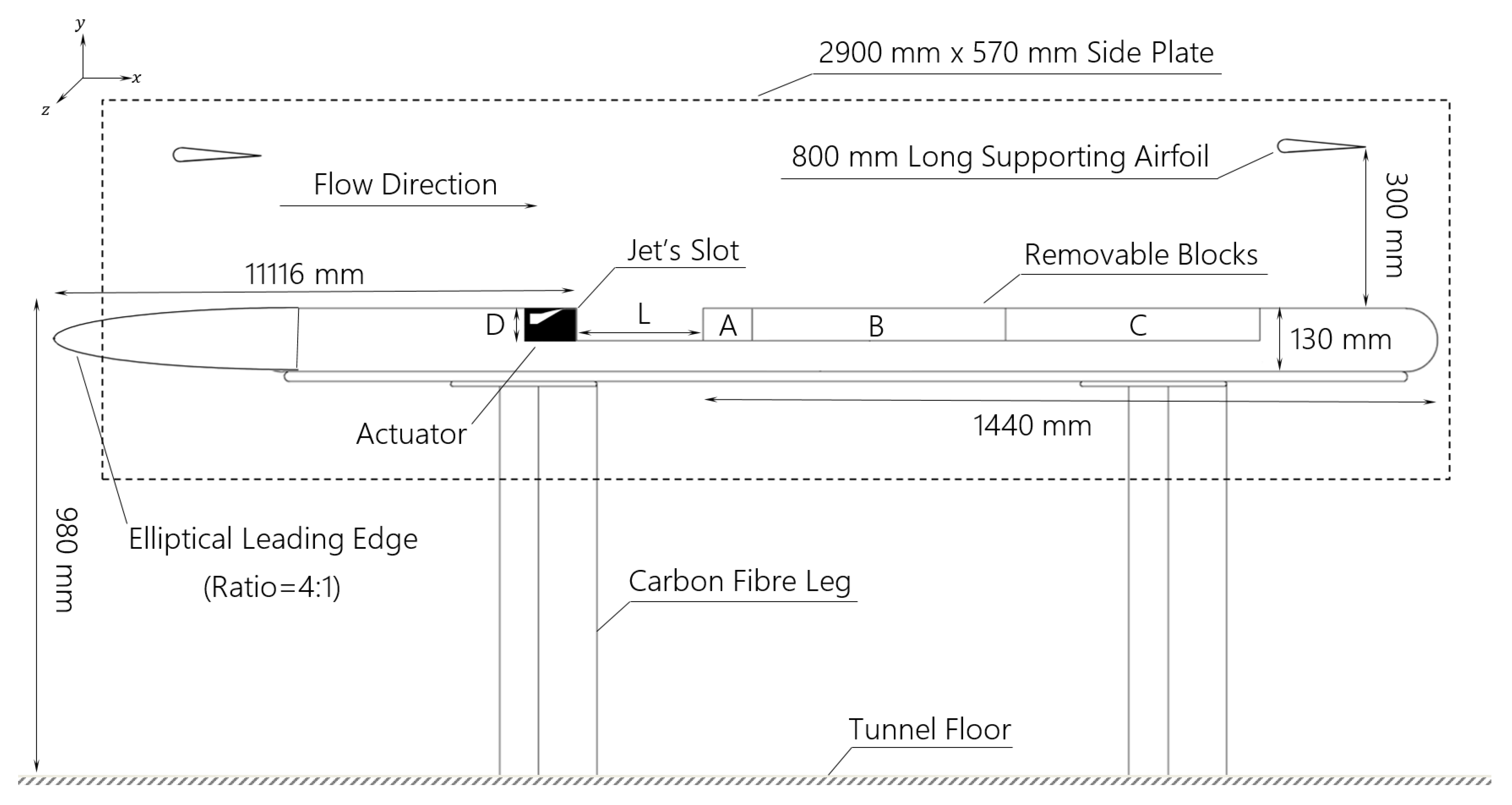
2. Experimental Setup

The experiments were carried out in the De Havilland tunnel at the University of Glasgow, which is a closed-return wind tunnel. The wind speed at the test section can reach up to approximately 76 m/s. The averaged turbulence intensities of the free stream are 1.82%, 1.95%, and 2.29% for free stream velocities of 11.1, 22.1, and 43.7 m/s, respectively. The main body of the cavity model is made of wooden panels and painted black to minimise laser reflections for the laser-based flow diagnostic methods. With a model span of 800 mm, the estimated model blockage ratio is approximately 5.9%.
As illustrated in Figure 2, the leading edge of the model has a smooth elliptic shape with a length of 400 mm and a width of 100 mm, which yields an axis ratio of 4. To allow full development to a turbulent boundary layer, a trip made of a sand-paper strip was glued to the model surface 600 mm upstream of the cavity leading edge. The experiments were performed on an open cavity with length L, depth D, and span W of 260 mm, 65 mm, and 800 mm, respectively. This yields an L / D ratio of 4 and a length to span ratio L / W of 0.325. The reference point for the coordinate system is located at the cavity leading edge. The x-axis corresponds to the streamwise direction, while the y-axis is in the vertical direction. The z-axis is along the span of the model.
The actuator was positioned at the cavity leading edge and fastened to the model by bolts screwed from underneath the model. To reduce manufacturing costs and air supply requirements, the actuator covers only the central portion of the cavity span. The actuator consists of an actuator housing, removable plastic insert, perforated tube, top plate, air chamber, a mesh, nozzle, knife edge, and jet outlet. The jet outlet is positioned at the cavity leading edge. The jet outlet is 1.85 mm wide and 400 mm long. The air-tight actuator housing, which was made of aluminium, is 65 mm high, 100 mm wide, and 420 mm long. The plastic inserts were made using a 3D printer and then surface-smoothed with sandpaper. Three design elements were added to the actuator to ensure a uniform jet along the span of the slot: (i) perforated tube to provide a uniform air supply, (ii) a chamber where the air mixes, and (iii) a mesh downstream of the air chamber to increase the pressure in the chamber, which enhances the mixing. Within the mid-span region of the jet ( 40 z / h 40 ), the velocity variation is approximately 5%.
The experiments were carried out at free stream velocity of 11.1 m/s, which corresponds to R e D 50,000 and R e θ = 1.28 × 10 3 . The upstream boundary layer was fully turbulent. For the jet-on cases, the jet’s bulk Reynolds number ( R e B u l k ), momentum flux per unit width (J), and momentum coefficient ( C μ ) are shown in Table 1. The jet momentum flux per unit width J is
J = b b ρ j U j 2 d y
where b, ρ j , and U j denote the half jet width, jet density, and jet streamwise velocity, respectively. The jet Reynolds number R e b u l k is based on the jet full width 2 b and the jet bulk velocity at x / h = 2.5 . The jet bulk velocity U B u l k is
U B u l k = b b ρ j U j d y b b ρ j d y
The surface oil flow visualisation technique was used to examine the flow on the cavity floor. Paraffin oil was mixed with fluorescent pigments with a mixture ratio (paraffin oil volume to fluorescent pigments volume) of 4 to 1. The mixture was then applied to the locations of interest as a thin layer by a paint roller. After a predetermined running time at the targeted speed, the shape of the formed patterns became time-independent. During the operation of the tunnel, the mixture is illuminated with a UV-LED light source, and images of the formed patterns are captured from the top of the test section by a Canon EOS 600D camera.
The jet’s bulk velocity was measured using constant temperature anemometry (CTA). For these measurements, a StreamLine-Pro system from Dantec Dynamics was used. The system consists of a hot-wire probe, CTA frame, analogue to digital converter (A/D), and a PC. The auxiliary components of the system include an automatic calibrator to calibrate the system and a traverse unit with its own controller to traverse the hot-wire probe. An x-wire miniature probe (55P61) was aligned parallel to the jet flow with each probe wire forming an angle of 45 with respect to the jet direction in order to measure the cross components of velocity. The probe was inserted into a straight probe support, which connects each probe wire to an individual module in the CTA frame via a short-length BNC cable. The bandwidth of the CTA module is typically 100–250 kHz. Each module consists of 1:20 general-purpose Wheatstone bridge and a feedback loop to convert the convected heat into voltage. The module also contains a signal conditioner, which filters the voltage signal and then amplifies it to the desired level. The signal is then sent to a 16 bit A/D converter board through a connection box. The A/D converter board (National Instrument PCI-6143) has 8 individual channels with a simultaneous sampling rate of 250 KS/s per channel and an analogue input resolution of 16 bit. This yields an analogue input resolution of 0.067 mV for input voltages between 0 and 5 volts. The A/D converter digitises the voltage signal and saves it onto the PC, where it is converted into a velocity signal using the calibration curve.
The sources of errors in CTA measurements include drift, calibration equipment, curve-fitting of the calibration curve, analogue to digital converter board resolution, probe positioning, temperature variations, ambient pressure variations, and gas composition. The relative expanded uncertainty for HWA velocity sample at normal experimental conditions is approximately 2.47%. The calculations of the relative expanded uncertainty for HWA velocity sample follow the instructions from the manufacturer of the HWA system [26].
A two-dimensional particle image velocimetry system (PIV), shown in Figure 3, was used to study the cavity velocity field. The laser beam is emitted from a dual-pulsed Litron Nd:YAG laser head, with a repetition rate of 200 Hz and wavelength of 532 nm. The laser head consists of two laser resonators, each emitting a laser beam. The laser beam is guided via a number of fixed mirrors into the laser sheet optics at the top of the test section, where the beam is expanded by a cylindrical lens into a thin laser sheet, which illuminates the mid-span of the cavity. PIV raw images are captured using a Phantom V341 digital high-speed video camera, placed perpendicular to the laser sheet. The camera is fitted with a 105 mm Sigma lens and equipped with CMOS sensor, which has a full resolution of 2560 × 1600 pixel at a frame rate of 10 to 800 frames/second. The camera was triggered and synchronised with the laser pulses by a high-speed controller.
Olive oil particles were generated from an Aerosol Generator PivPart160 atomiser and injected into the wind tunnel as tracer particles before acquiring the images. The atomiser generates particles with a mean diameter of 1 μ m. The Stokes number of the particles is much smaller than 0.1; hence, the tracking error of the particles is negligible in the current study. Each interrogation area contained a considerable number of seeding particles, which enhances the signal-to-noise ratio [27]. Before acquiring the images, sufficient time was allowed for the particles to distribute homogeneously in the wind tunnel.
Davis 8 software from LaVision was used to process and post-process the raw images. The images were processed using a multi-pass cross-correlation approach with decreasing interrogation windows from 32 × 32 pixels (2 passes) to 16 × 16 pixels (3 passes). The size of the interrogation windows could not be reduced further due to the limited number of particles. However, the interrogation windows were overlapped by 50%, which increased the spatial resolution to approximately 1 mm × 1 mm. Basic filters and post-processing tools, including correlation value limit, median filter, peak ratio, and 3 × 3 pixels smoothing filter, were applied to the processed images.
The uncertainty for time-averaged two-dimensional PIV measurements is due to the PIV equipment σ E , the seeding particle lag σ L , the sampling size σ S , and the processing algorithm σ P [28]. The combined uncertainty for the time-averaged PIV measurements is 3.45%, where the combined uncertainty is
σ T = σ E 2 + σ L 2 + σ S 2 + σ P 2 = 0 + 0 + 3.39 2 + 1 2 = 3.45 %
Pressure measurements were utilised to carry out the spectral analysis of the wall pressure fluctuations. Pressure taps were drilled at different locations along the cavity mid-span. Only one tap at a time was used for measurements. The tap was connected to a differential pressure transducer via a hypodermic and a 1 mm diameter flexible tube of a total length of approximately 85 mm. The shortest possible flexible tube was used to minimize the attenuation effect of high frequencies. The second port of the transducer is open to the atmosphere (outside the wind tunnel), which is the reference pressure. A 5-core cable connected the transducer to a DC voltage supply module (NI 9246), a data acquisition module (NI 9205), and a grounding connection. The two modules were inserted into a grounded compact chassis (NI cDAQ-9178), which is connected via a USB connection to a computer and controlled with LabVIEW program.
The differential pressure transducer (First Sensor-LBA series) is a bi-directional transducer with an operating pressure of 0 to 5 mbar and a full-scale output voltage of 0.5 to 4.5 volts. The total accuracy of the transducer is ±1.5% of the sum of the pressure reading and the full-scale span. The pressure transducer has a maximum frequency response of 1 kHz.
The unsteady pressure measurements for the power spectral density (PSD) were performed at x / L of 0.5 and 0.75. A total of 4.4 million samples were acquired for these measurements at a sampling rate of 20 kHz. Matlab was used to generate the power spectral density (PSD) using Welch’s algorithm [29]. In order to minimise the effect of spectral leakage, the pressure time series was multiplied by a window function before executing fast Fourier transform (FFT) algorithm [30]. A total of 440 windows were used for averaging. A 10,000-point FFT with Hanning window was used to compute the power spectral density. Hanning window is usually used for random and periodic data because it has a moderate frequency resolution and amplitude uncertainty compared to other types of window functions. With these parameters, the margin of error for the 95% confidence level is between −0.42% and +0.44% of the spectral peak amplitude.

3. Results and Discussion

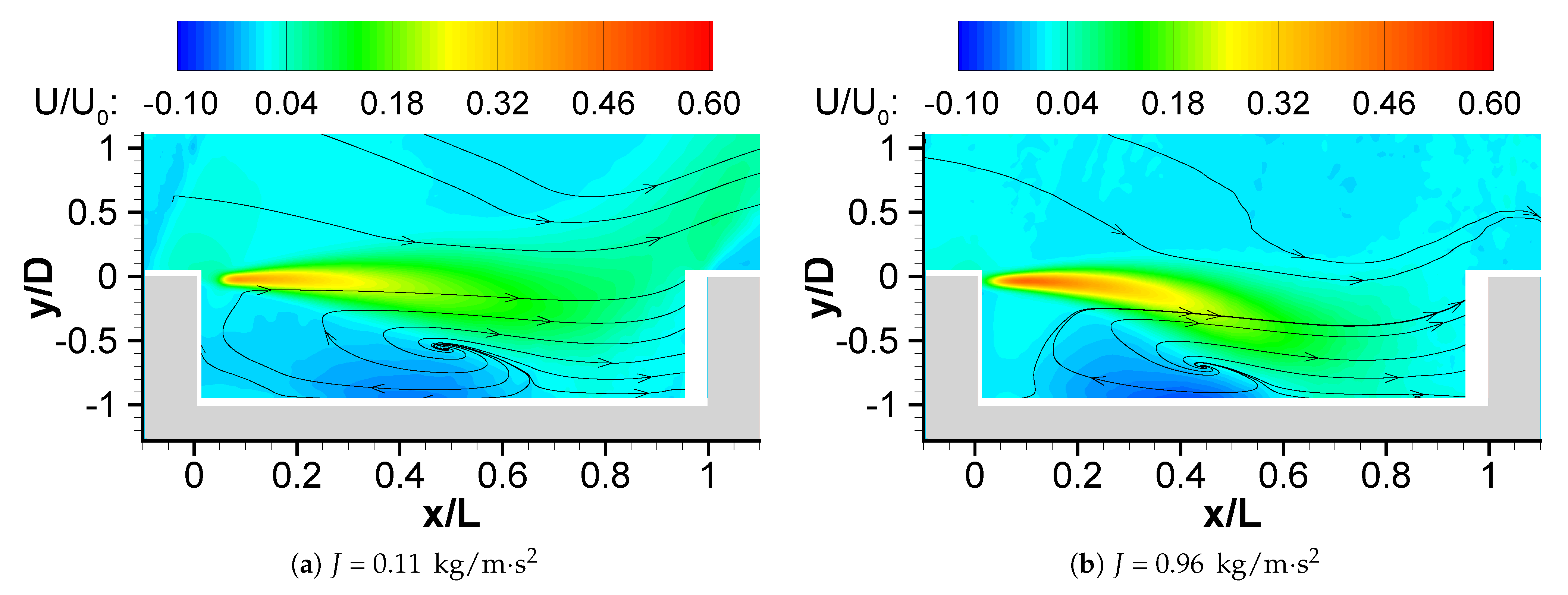
3.1. Jet Behaviour under Quiescent Conditions

The jet characteristics were examined in two stages: (i) CTA measurements for the jet without the cavity model and (ii) PIV measurements for the jet with the cavity model. Both stages were performed under quiescent conditions. The first stage aims to calculate the jet’s bulk velocity and the jet angle, while the second stage aims to examine the jet behaviour in the cavity under quiescent conditions. Figure 4 shows the vertical shift of the jet centre along the x-axis for the jet without the cavity model. In this figure, y c denotes the local y-position of the jet centre, while y x / h = 2.5 indicates the y-position of the jet centre at x / h = 2.5 , which is the closest position to the slot that the CTA probe could reach without blocking the jet or damaging the CTA probe. Using the horizontal distance and the maximum vertical shift provided in the figure, the maximum estimated jet angle is 2.2 . This angle is negligible and within the uncertainty of the CTA probe angle. Thus, it is concluded that the centreline of the jet is approximately parallel to the x-axis.
Installing the actuator inside the cavity model yields a significant change in the jets’ angle. Figure 5 illustrates the time-averaged velocity streamlines and U / U 0 contours for J = 0.11 kg/m·s 2 and J = 0.96 kg/m·s 2 . For J = 0.11 kg/m·s 2 , the jet deflects slightly towards the cavity floor, and then it deflects upwards as it approaches the cavity trailing edge. A similar behaviour was noted for 0.44 kg/m·s 2 . For J = 0.96 kg/m·s 2 , the jet deflects downwards until it reattaches at the cavity floor, and then the jet impinges on the cavity trailing edge and deflects upwards. At the same time, a portion of the jet is recirculated towards the cavity leading.
The jet deflection towards the cavity floor at J = 0.96 kg/m·s 2 is attributed to the coanda effect. As the characteristic jet velocity (or J) increases, the jet entrains more fluid from the cavity [31]. As a result, the static pressure at the cavity floor decreases, until it reaches a threshold value. Beyond this point, the pressure force causes the jet to deflect towards the cavity floor. Figure 6 shows the time-averaged V velocity distribution along the cavity floor ( y / D = 0.9 ) for different J values. The positive V velocity indicates upward fluid movement or jet entrainment, while the negative V velocity indicates a downward fluid movement. The jet entrainment at J = 0.11 kg/m·s 2 and J = 0.44 kg/m·s 2 is quite small. Increasing J to 0.96 kg/m·s 2 yields a significant increase in the entrainment at the upstream half ( 0 x / L 0.4 ), which forces the jet to deflect downwards. As the jet deflects and reattaches onto the cavity floor, the sign of V shifts from positive to negative. In summary, the jet is parallel to the x-axis. However, installing the jet in the cavity model causes it to deflect downwards towards the cavity floor due to the coanda effect. If this effect persists in the dynamic conditions (wind tunnel is on), jet deflection will increase the cavity return flow instead of reducing it.

3.2. Time-Averaged Flow Field

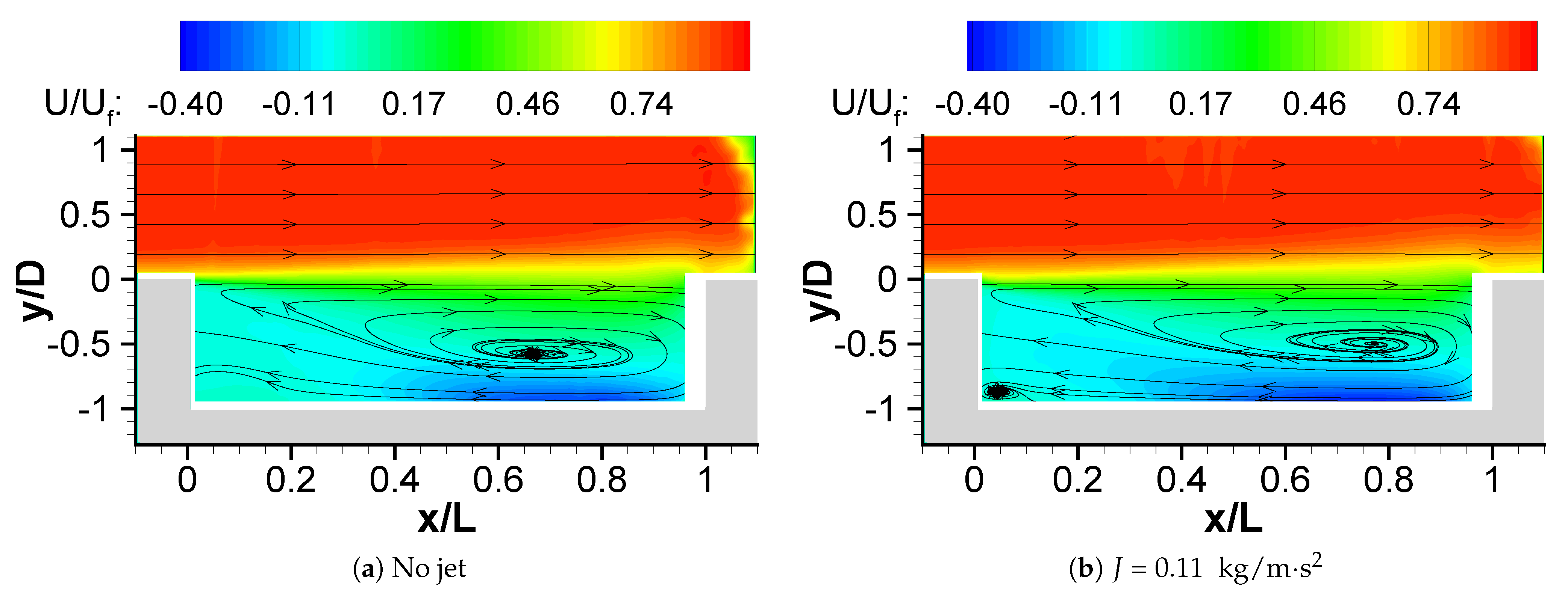
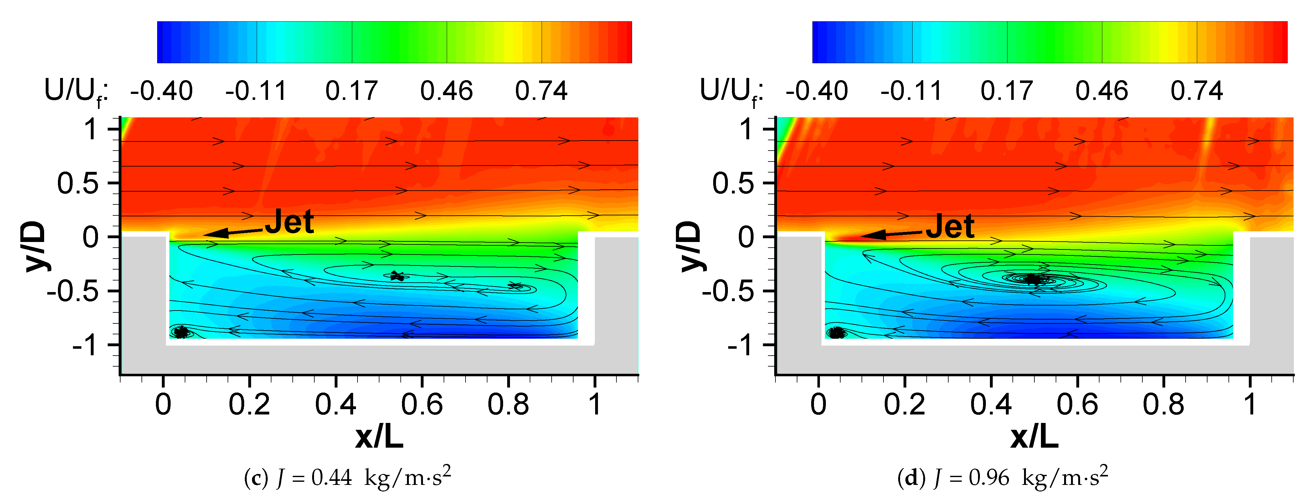
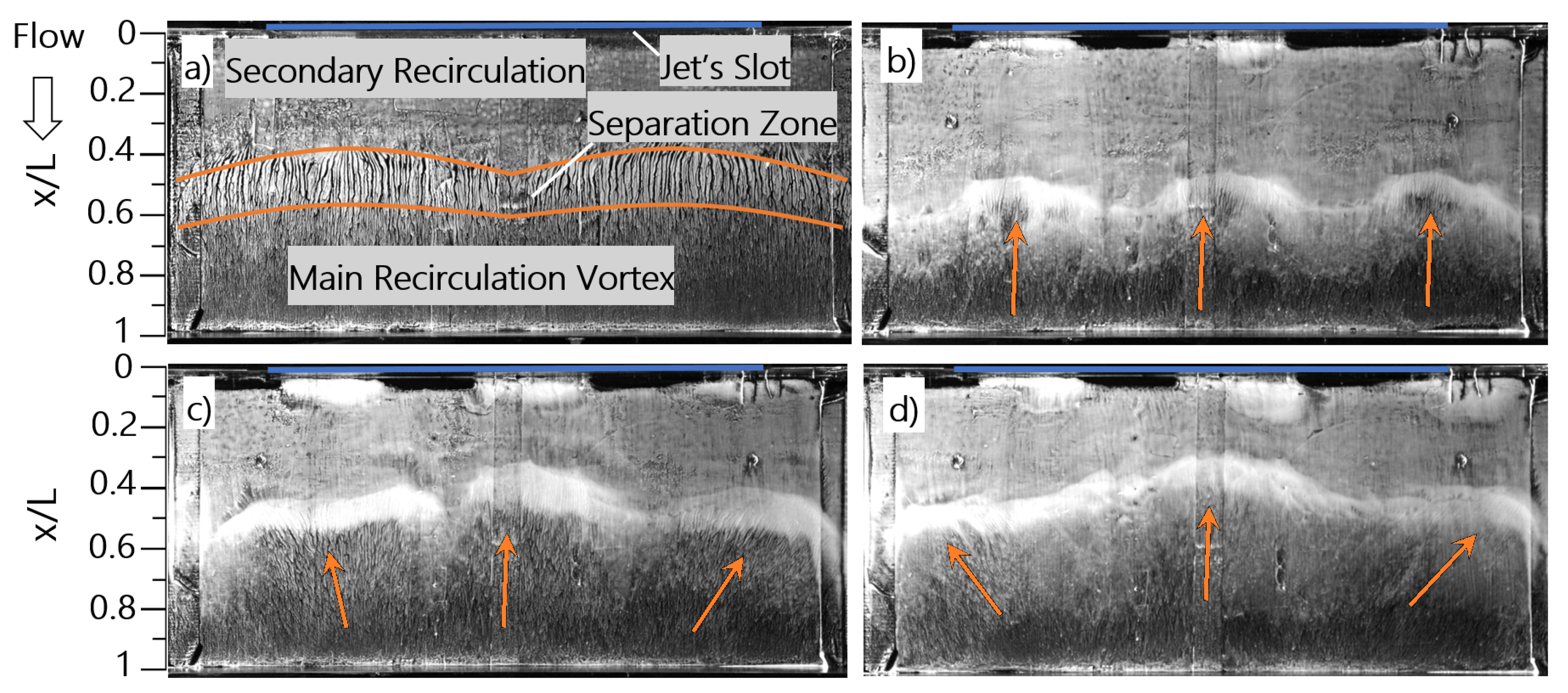
3.2.1. Jet Impact on the Cavity Flow Topology

The time-averaged U / U f fields in the cavity for the no-jet and jet-on cases are shown in Figure 7. Forcing the jet at J = 0.11 kg/m·s 2 does not yield significant changes in the velocity field. As J increases to 0.44 kg/m·s 2 , the jet penetration through the shear layer appears clearly at the cavity leading edge region, as indicated by the arrow in Figure 7c. The centre of the main recirculation vortex shifts upstream, while the return flow rate increases. Increasing J to 0.96 kg/m·s 2 causes a clearer jet penetration effect and shifts the main recirculation vortex (centred at x / L 0.5 ) further towards the cavity leading edge due to the increase in the return flow rate, as illustrated in Figure 7d. In contrast, increasing the jet’s momentum flux in the simulation of Suponitsky et al. [25] at R e D of 5000 caused a reduction in the return flow rate and suppression in oscillations of the cavity separated shear layer. Therefore, the increase in the return flow rate in the current study is believed to enhance separated shear layer oscillations.

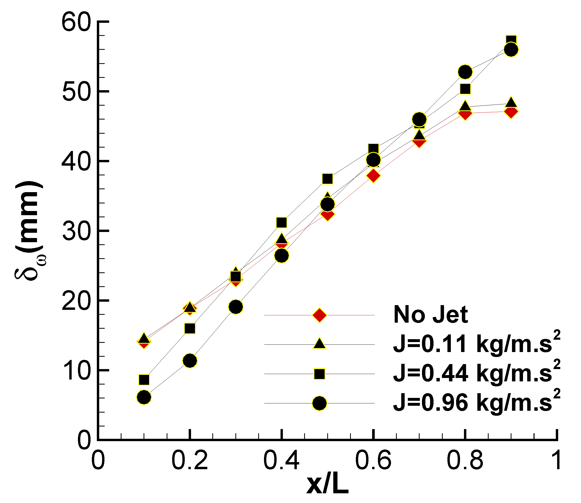
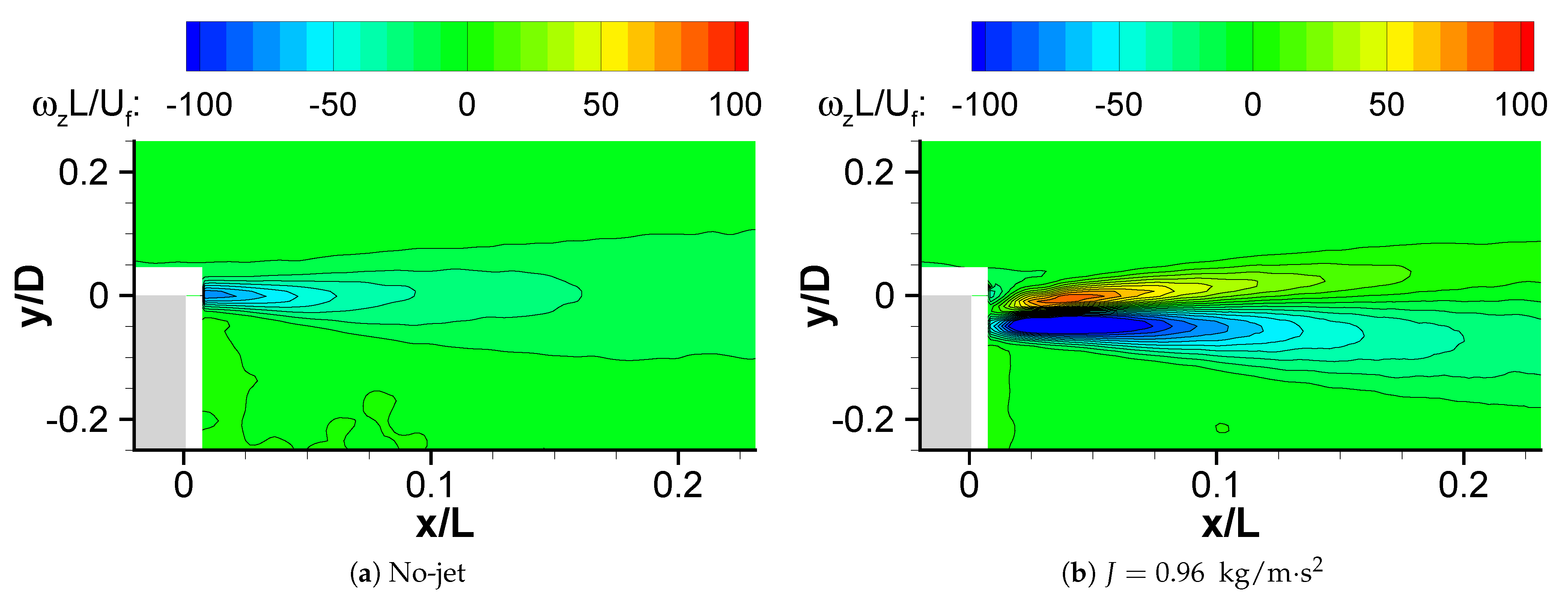
3.2.2. Jet Impact on the Cavity Separated Shear Layer

Figure 8 shows the vorticity thickness of the cavity shear layer along the x-axis. The vorticity thickness δ ω is defined as
δ ω = U 2 U 1 { U y } m a x
where { U y } m a x is the local maximum velocity gradient across the mixing layer, while U 2 is the free stream velocity and U 1 = 0 . Based on this figure, the growth rates of the cavity separated shear layer for the no-jet and jet-on cases are estimated in Table 2. As evident from the table, the growth rate increases with J. This increase is attributed to two factors: (i) the transfer of jet momentum to the lower part of the cavity separated shear layer, which will be discussed later, and (ii) the strong interaction between the jet and the cavity trailing edge, which increases the V component of velocity and hence increases the thickness of the cavity separated shear layer at this region.
To further investigate the jet impact on the separated shear layer, Figure 9 shows the time-averaged PIV raw images and U / U f profiles at different axial stations for different values of J. To show the U / U f profiles clearly, they are separated by equal margins along the x-axis of the plot. At J = 0.11 kg/m·s 2 , the jet completely mixes with the cavity flow near the cavity leading edge and hence has almost no influence on the velocity profiles downstream, as illustrated in Figure 9a. However, at J = 0.44 kg/m·s 2 , the jet penetrates the cavity separated shear layer. As the jet expands downstream, the velocity difference decreases until the two profiles collapse into one profile at x / L 0.6 . At J = 0.96 kg/m·s 2 , the penetration effect is stronger, as shown in Figure 9d. Even at J = 0.96 kg/m·s 2 , the figure does not show any downward deflection in the cavity separated shear layer, which was observed previously in Figure 5 for the quiescent condition due to the coanda effect. However, at this J value, the lower side of the jet grows faster than the upper side. The difference in the jet’s growth rate between the two halves of the jet is because the upper side of the jet is in contact with the relatively fast-moving free stream, while the lower side of the jet is in contact with the relatively slow-moving cavity flow. As a result, the jet’s growth rate on the lower side is larger than that of the upper side. This is because the strongly advected side of the jet (the upper side) has difficulty in entraining the free stream fluid into the jet, as the jet momentum at this side of the jet is relatively small compared to the momentum of the free stream, and vice versa for the weakly advected side of the jet (the lower side) [32]. This is consistent with reported studies on jet interaction in a co-flowing free stream, such as the studies of Ben Haj Ayech et al. [33] and Kalifa et al. [34]. It is also important to note that the jet causes a reduction in the streamwise velocity near the cavity trailing edge (region “C”), as demonstrated in Figure 9d. This reduction is attributed to the increase of the upward V velocity at the cavity trailing edge, which impedes the flow of the shear layer and increases the thickness of the the cavity separated shear layer.

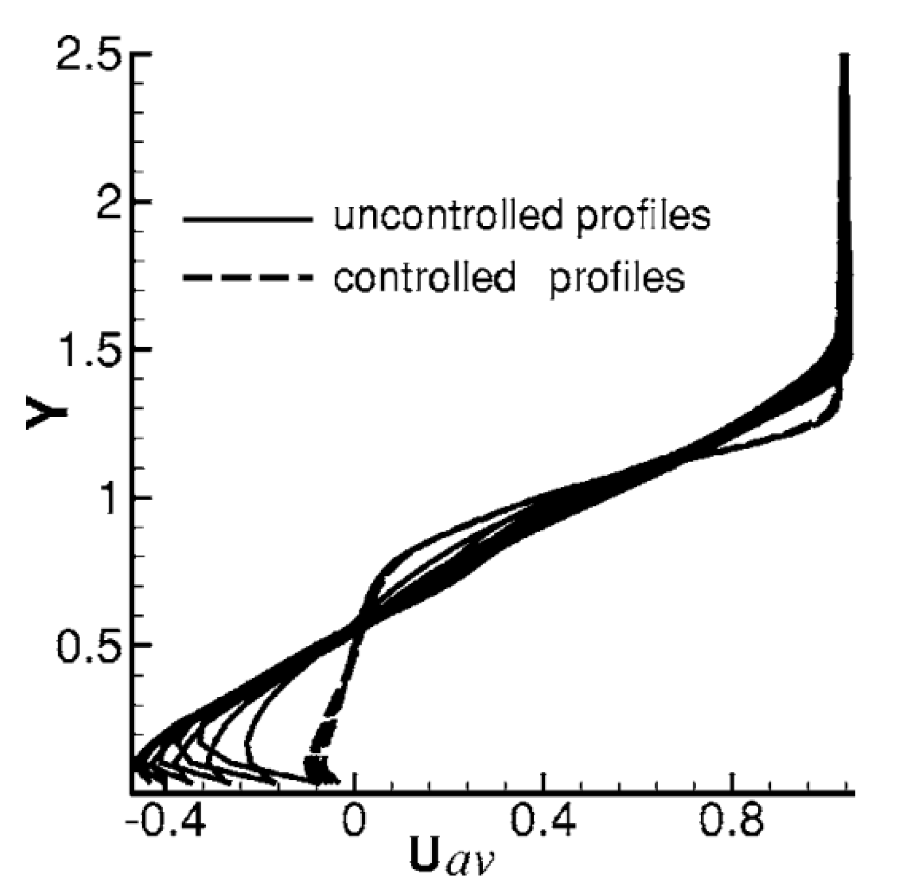
3.2.3. Jet Impact on the Return Flow

Figure 10 shows the time-averaged V / U f along the centre of the main recirculation vortex. As J increases, the jet impingement at the cavity trailing edge increases the return flow velocity and pushes the main recirculation vortex upstream. As a result, more return flow impacts the cavity leading edge region. However, increasing J from 0.44 kg/m·s 2 to 0.96 kg/m·s 2 does not produce a significant increase in the amount of the return flow impacting the cavity leading edge.
The increase in the return flow velocity causes the separation point to move towards the cavity leading edge. Figure 11 shows the distribution of U / U f along the cavity floor ( y / D = 0.9 ). The streamwise locations X R 1 , X R 2 , and X R 3 , 4 denote the separation point for the no-jet, J = 0.11 kg/m·s 2 , and J = 0.44 kg/m·s 2 cases, respectively. The results show that for J = 0.11 kg/m·s 2 , the separation point is displaced upstream from x / L 0.2 to x / L 0.1 . Increasing J to 0.44 kg/m·s 2 slightly shifts the separation point to x / L 0.07 . There is almost no change in the position of the separation point between J = 0.44 kg/m·s 2 and J = 0.96 kg/m·s 2 cases.
The small difference in the return flow rate and position of the separation point between the J = 0.44 kg/m·s 2 and J = 0.96 kg/m·s 2 cases is attributed to the divergence of the return flow. Figure 12 shows the images of the surface oil flow visualisations for the no-jet and jet-on cases. The images are for the central portion on the cavity. The blue line at the cavity leading edge indicates the slot. At J = 0.11 kg/m·s 2 , the return flow is parallel to the x-axis, as evident from Figure 12b. As J increases, the return flow starts to diverge towards the side walls. This divergence increases with J, as illustrated in Figure 12c,d. This divergence is attributed to the impingement of the jets at the cavity trailing edge. This impingement raises the stagnation pressure at the mid-span of the cavity compared to the side regions, where the jet is not applied. As a result, the return flow diverges towards the side regions of the cavity. Despite this flow divergence, the return flow at the mid-span region remains parallel to the x-axis, and hence, the flow at this region, where the PIV and pressure measurements are acquired, is likely to be two-dimensional.

3.3. Jet Impact on the Oscillations of the Cavity Separated Shear Layer

The jet also has an impact on the oscillations and the large coherent structures of the cavity separated shear layer. The unsteady wall pressure spectral density (PSD) at x / L = 0.5 for different J values is illustrated in Figure 13. As evident from the figure, a sharp spectral peak exists at S t 3 . This peak coincides with the frequency of the first acoustic transversal mode. The transversal acoustic mode has been observed by Ziada et al. [35], Debiasi and Samimy [22], Little et al. [23], Chan et al. [36], and Ashcroft and Zhang [11]. Although the jet supplies the cavity flow with additional disturbances, the spectral peak at S t 3 is not affected. This proves again that this spectral peak is not related to the cavity separated shear layer but to the acoustic transversal mode.
The pressure spectral density (PSD) does not reveal any peak associated with the oscillations of the cavity separated shear layer. This is probably because the oscillations are random and not organised. The randomness of cavity oscillations in the current study is perhaps due to the large cavity length. As the cavity length increases, the cavity shear layer oscillations jump from lower oscillation modes to higher modes until the oscillations become irregular at a certain threshold value [37]. For axi-symmetrical cavities, the cavity length threshold was found by Gharib and Roshko [38] and Sarohia [37] to be L / θ 0 = 155 and L / δ 0 18 . The former threshold value was obtained at a Reynolds number based on the model diameter R e d i a of 2.4 × 10 4 , while the latter value was obtained at R e d i a of 2 × 10 4 and 10 5 . The upstream momentum boundary layer thickness θ 0 and boundary layer thickness δ 0 in the present study are 1.69 mm and 13.9 mm, respectively. Thus, for the current study, the cavity length is approximately at the threshold point for both reported values ( L / θ 0 154 and L / δ 0 = 18.7 ).
Figure 13 also shows that the turbulence broadband level increases with J. This is due to the relatively small-scale disturbances generated by the jet, which are responsible for the rise in the turbulence fluctuation. The increase in the turbulence fluctuation is also evident by the increase in the Reynolds shear stresses. Figure 14 shows the dimensionless time-averaged Reynolds shear stress < u v > / U f 2 for the no-jet (baseline) and jet-on cases. As illustrated in the figure, increasing J yields a substantial increase in the Reynolds shear stress in the shear layer. Figure 15 shows the time-averaged vorticity of the shear layer with no-jet and with jet ( J = 0.96 kg/m·s 2 ). The presence of the jet generates two regions of narrow thickness and high vorticity. These opposite-vorticity regions are generated due to the higher velocity at the jet centre compared to the velocity at the jet boundaries. In these two regions, small-scale counter-rotating vortical structures are continuously shed due to Kelvin–Helmholtz instability [39]. Although these small-scale structures might have a short life-span, they increase the fluctuation level and affect the large coherent vortical structures in the cavity separated shear layer.
In order to study the impact of the jet on the large coherent vortical structures, these structures are further examined. To reveal these structures in the cavity separated shear layer, the fluctuating velocity flow fields were generated. The fluctuating velocity flow fields were produced by subtracting the instantaneous flow fields from the time-averaged field. Afterwards, a spatial filter with a Gaussian kernel was used to filter out small structures, and hence it generates a clearer visualisation of the large coherent structures. Figure 16a shows the unfiltered fluctuating velocity field. Two large vortical structures appear: one centred at ( x / L 0.4, y / D 0.3) and the other centred at ( x / L 0.8, y / D 0.2). Applying the spatial filter with a Gaussian kernel size of 18 mm × 18 mm (Figure 16b) provides a clearer visualisation of vortical structures. Increasing the filter size to 27 mm × 27 mm (Figure 16c) enhances the clarity of the large vortical structures further. A further increase in the kernel size (Figure 16d) filters out some flow details without improving the clarity of the large vortical structures. Thus, it was decided to implement the spatial filter with a Gaussian kernel size of 27 mm × 27 mm. Using this method, 400 sequential images were examined to count the large coherent vortical structures passing over the cavity trailing edge.
Figure 17 shows the vortex count of the large coherent vortical structures passing over the cavity trailing edge for R e θ = 1.28 × 10 3 . As illustrated in the figure, increasing the jet’s momentum flux makes the formation of large coherent vortical structures more intermittent. This suppression effect is probably because the jet supplies the cavity with relatively small-scale disturbances. As J increases, the jet populates the separated shear layer with these small-scale disturbances, which impede the formation of the large coherent vortical structures. A similar finding was reported by Smith and Glezer [40], who examined the interaction between a conventional rectangular (primary) air jet and a co-flowing synthetic jet at a Reynolds number based on the exit jet velocity of 300–440. In their study, the spectrum analysis showed that the Kelvin–Helmholtz (K-H) instabilities (which lead to the formation of the vortical structures in the separated layer) were suppressed particularly in the jet–jet interaction region, as the large vortical structures were replaced by small-scale disturbances.

3.4. Further Discussion

Although the momentum coefficient C μ in the current study (between 0.57% and 5.04%) significantly exceeds the threshold value of C μ found by Suponitsky et al. [25], C μ 0.11 % , steady blowing from the cavity leading edge does not yield any noticeable improvements in the stability of the cavity separated shear layer. According to Suponitsky et al. [25], the effectiveness of this control method is linked to the suppression of the cavity return flow velocity. To investigate this further, the dimensionless streamwise velocity profiles from the current study (Figure 9d) are compared with the velocity profiles from the simulation of Suponitsky et al. [25] in Figure 18. Figure 9d shows the velocity profiles along the cavity length, while Figure 18 shows the profiles in the last quarter of the cavity 3 < L / D < 4 for flow controlled by the injection and suction. According to Suponitsky et al. [25], suction at the cavity trailing edge does not have a significant effect of on the cavity flow field, but it provides a mass source for the jet injection. Therefore, it can be assumed that Figure 18 also represents the controlled case by injection from the cavity leading edge. As illustrated in Figure 9d, adding the jet in the current study increases the thickness and streamwise velocity of the cavity separated shear layer, especially at the lower portion of the cavity separated shear layer (below y / d = 0 ). As a result, the return flow velocity increases. In contrast, Figure 18 illustrates that the jet in Suponitsky et al.’s [25] work reduced the thickness of the cavity separated shear layer. The jet also reduced the streamwise velocity at the lower portion of the cavity separated shear layer (below Y = 1 ). This is the justification for the reduction in the cavity return flow velocity in the study of Suponitsky et al. [25], though the authors did not provide a detailed justification for this reduction.
The contradicting results between the two studies are attributed to two controlling parameters: (i) the ratio of the slot height to the boundary layer momentum thickness h / θ and (ii) the velocity ratio ( U j / U f ). In the current study h / θ = 1.09 , while U j / U f is between 0.8 to 1.8. In the work of Suponitsky et al. [25], h / θ = d / θ × h / d = 68.5 × 0.1 = 6.85 , whereas U j / U f is between 0.15 and 0.4. If we assume that the boundary layer thickness is eight times the momentum thickness, then the slot height in the study of Suponitsky et al. [25] is as thick as the cavity separated shear layer at the cavity leading edge. On the other hand, the slot height in the current study is much smaller than the cavity separated shear layer. Forcing the jet at a high velocity ratio through a narrow slot yielded a steep and highly unstable velocity profile as shown in Figure 9d. This enhances mixing between the jet and the cavity separated shear layer and hence increases the growth rate of the cavity separated shear layer and the velocity of the cavity return flow. One the other hand, the jet in the study of Suponitsky et al. [25] was forced through a wider slot and at a smaller velocity ratio. This produced less steep and more stable velocity profiles (as shown in Figure 18). This reduced the thickness of the cavity separated shear layer and the momentum of the lower part of the cavity separated shear layer (below Y = 1 ). This finding is consistent with the simulation of Hnaien et al. [41] for the interaction of two plane parallel jets separated by a small gap. The study was performed at a jet Reynolds number of 6000. The authors concluded that the weak jet exercises some resistance on the strong jet and hence reduces its growth rate. In contrast, the strong jet increases the momentum of the weak jet and thus increases its growth rate. Although the aforementioned study is between two jets and the current study is between a separated shear layer and a jet, both jet and separated shear layer are considered as shear flows. Another factor to be taken into account is the impact of the jet at the cavity trailing edge. In the work of Suponitsky et al. [25], the jet modified the velocity profiles at the cavity trailing edge region. On the other hand, no significant change in velocity profiles in this region was observed in the current study. This perhaps is due to the intensive mixing between the jet and the cavity separated shear layer or due to the large cavity length which allowed the jet to mix with the cavity separated shear layer and diminished upstream of the cavity trailing edge. In summary, the control effectiveness of the jet blowing from the cavity leading edge requires a careful selection of U j / U f and h / θ to stabilise the cavity separated shear layer. Reducing the cavity length can help to avoid the diminishing of the jet upstream of the cavity trailing edge. To support this conclusion, we recommend a parametric study on the effect of U j / U f and h / θ and cavity length (with constant L / D and C μ ) on the control effectiveness of the jet blowing from the cavity leading edge.

4. Conclusions

The impact of the cavity leading edge blowing was investigated at R e D 50,000 and 0.11 kg/m·s 2 J 0.96 kg/m·s 2 . The main objective of this control method is to reduce the cavity return flow by isolating the cavity separated shear layer from the recirculation zone in order to stabilise the cavity separated shear layer. Although Suponitsky et al. [25] found that this control method was highly effective in suppressing cavity separated shear layer oscillations at a relatively low Reynolds number ( R e D 5000 ), the current study found that this method does not yield any noticeable improvement in the stability of the cavity separated shear layer. The jet increased the thickness of the lower part of the cavity separated shear layer, and hence the cavity return flow increased. The jet also populates the cavity separated shear layer with a large number of relatively small-scale disturbances originating from the jet itself. As a result, the broad band level of the pressure spectral density and Reynolds shear stress increased significantly within the cavity separated shear layer. On the other hand, as the jet’s momentum flux increases, the shedding of the large coherent vortical structures becomes more intermittent. This is probably due to the presence of the jet’s small-scale disturbances, which impede the formation of the large vortical structures.

Author Contributions

Conceptualization, N.A.H., K.K. and H.Z.-B.; methodology, N.A.H., K.K. and H.Z.-B.; formal analysis, N.A.H. and H.Z.-B.; resources, N.A.H., K.K. and H.Z.-B.; data curation, N.A.H.; writing—original draft preparation, N.A.H.; writing—review and editing, N.A.H., K.K., H.Z.-B.; funding acquisition, K.K.; supervision K.K., H.Z.-B. All authors have read and agreed to the published version of the manuscript.

Funding

This research received no external funding.

Institutional Review Board Statement

Not applicable.

Informed Consent Statement

Not applicable.

Data Availability Statement

Not applicable.

Acknowledgments

We are sincerely grateful for all the support from the technical staff and the colleagues who helped in completing this work. The support of the EPSRC-funded National Wind Tunnel Facility project (grant EP/L024888/1) is gratefully acknowledged.

Conflicts of Interest

The authors declare no conflict of interest.

Nomenclature

bLocal jet half width [m]
C μ Jet’s momentum coefficient [%]
DCavity depth [m]
fRepetition rate of the particle image velocimetry [Hz]
hCharacteristic slot width [m]
JJet’s momentum flux per unit width [kg/m·s 2 ]
LCavity length [m]
L E Cavity leading edge
MMach number
R e B u l k Reynolds number based on the bulk velocity of the jet
R e D Reynolds number based on the cavity depth
R e d i a Reynolds number based on the model diameter
R e θ Reynolds number based on the boundary layer momentum thickness
S t Non-dimensional frequency S t = f L / U f
tTime [s]
T E Cavity trailing edge
< u >Time-averaged streamwise velocity fluctuation [m/s]
UThe streamwise velocity [m/s]
U 0 Jet exit velocity [m/s]
U f The free stream velocity [m/s]
< v >Time-averaged normal-to-wall velocity fluctuation [m/s]
VNormal-to-wall velocity [m/s]
WCavity width [m]
xThe streamwise distance from the reference point [m]
yThe vertical distance from the reference point [m]
zThe spanwise distance from the reference point [m]
δ ω The vorticity thickness [m]

References

  1. Srinivasan, G.R. Acoustics and unsteady flow of telescope cavity in an airplane. J. Aircr. 2000, 37, 274–281. [Google Scholar] [CrossRef]
  2. Vakili, A.D.; Gauthier, C. Control of cavity flow by upstream mass-injection. J. Aircr. 1994, 31, 169–174. [Google Scholar] [CrossRef]
  3. Gai, S.L.; Soper, T.J.; Milthorpe, J.F. Shallow Rectangular Cavities at Low Speeds Including Effects of Yaw. J. Aircr. 2008, 45, 2145–2150. [Google Scholar] [CrossRef]
  4. Ziada, S.; Lafon, P. Flow-excited acoustic resonance excitation mechanism, design guidelines, and counter measures. Appl. Mech. Rev. 2014, 66. [Google Scholar] [CrossRef]
  5. He, B.; Xiao, X.; Zhou, Q.; Li, Z.-H.; Jin, X.-S. Investigation into external noise of a high-speed train at different speeds. J. Zhejiang Univ. Sci. A 2014, 15, 1019–1033. [Google Scholar] [CrossRef] [Green Version]
  6. Ukeiley, L.; Murray, N. Velocity and surface pressure measurements in an open cavity. Exp. Fluids 2005, 38, 656–671. [Google Scholar] [CrossRef]
  7. Tuna, B.A.; Tinar, E.; Rockwell, D. Shallow flow past a cavity: Globally coupled oscillations as a function of depth. Exp. Fluids 2013, 54, 1586. [Google Scholar] [CrossRef]
  8. Rockwell, D.; Knisely, C. The organized nature of flow impingement upon a corner. J. Fluid Mech. 1979, 93, 413. [Google Scholar] [CrossRef]
  9. Lin, J.C.; Rockwell, D. Organized Oscillations of Initially Turbulent Flow past a Cavity. AIAA J. 2001, 39, 1139–1151. [Google Scholar] [CrossRef] [Green Version]
  10. Yan, P.; Debiasi, M.; Yuan, X.; Little, J.; Ozbay, H.; Samimy, M. Experimental Study of Linear Closed-Loop Control of Subsonic Cavity Flow. AIAA J. 2006, 44, 929–938. [Google Scholar] [CrossRef] [Green Version]
  11. Ashcroft, G.; Zhang, X. Vortical structures over rectangular cavities at low speed. Phys. Fluids 2005, 17, 015104. [Google Scholar] [CrossRef]
  12. Rockwell, D.; Naudascher, E. Self-Sustained Oscillations of Impinging Free Shear Layers. Annu. Rev. Fluid Mech. 1979, 11, 67–94. [Google Scholar] [CrossRef]
  13. Rossiter, J.E. Wind Tunnel Experiments on the Flow over Rectangular Cavities at Subsonic and Transonic Speeds; Ministry of Aviation, Royal Aircraft Establishment, RAE Farnborough: Farnborough, UK, 1964. [Google Scholar]
  14. Patricia, J.; Block, W.; Heller, H. Measurements of Farfield Sound Generation from a Flow-Excited Cavity; NASA: Washington, DC, USA, 1975. [Google Scholar]
  15. Rockwell, D.; Naudascher, E. Review—Self-sustaining oscillations of flow past cavities. Trans. ASME J. Fluids Engng 1978, 100, 152–165. [Google Scholar] [CrossRef]
  16. Sarno, R.L.; Franke, M.E. Suppression of flow-induced pressure oscillations in cavities. J. Aircr. 1994, 31, 90–96. [Google Scholar] [CrossRef]
  17. Sarohia, V.; Massier, P.F. Control of cavity noise. J. Aircr. 1976, 14, 833–837. [Google Scholar] [CrossRef]
  18. Cattafesta, L.N.; Song, Q.; Williams, D.R.; Rowley, C.W.; Alvi, F.S. Active control of flow-induced cavity oscillations. Prog. Aerosp. Sci. 2008, 44, 479–502. [Google Scholar] [CrossRef]
  19. Franke, M.; Carr, D. Effect of geometry on open cavity flow-induced pressure oscillations. In Proceedings of the 2nd Aeroacoustics Conference, Hampton, VA, USA, 24–26 March 1975. [Google Scholar] [CrossRef]
  20. Ethembabaoglu, S. On the Fluctuating Flow Characteristics in the Vicinity of Gate Slots. Ph.D. Thesis, University of Trondheim, Trondheim, Norway, 1973. [Google Scholar]
  21. Cattafesta, L.N., III; Williams, D.R.; Rowley, C.W.; Alvi, F.S. Review of Active Control of Flow-Induced Cavity Resonance. In Proceedings of the 33rd AIAA Fluid Dynamics Conference, Orlando, FL, USA, 23–26 June 2003. [Google Scholar] [CrossRef]
  22. Debiasi, M.; Samimy, M. Logic-Based Active Control of Subsonic Cavity Flow Resonance. AIAA J. 2004, 42, 1901–1909. [Google Scholar] [CrossRef] [Green Version]
  23. Little, J.; Debiasi, M.; Caraballo, E.; Samimy, M. Effects of open-loop and closed-loop control on subsonic cavity flows. Phys. Fluids 2007, 19, 065104. [Google Scholar] [CrossRef]
  24. Rowley, C.W.; Williams, D.R. Dynamics and Control of High-Reynolds-Number Flow Over Open Cavities. Annu. Rev. Fluid Mech. 2006, 38, 251–276. [Google Scholar] [CrossRef]
  25. Suponitsky, V.; Avital, E.; Gaster, M. On three-dimensionality and control of incompressible cavity flow. Phys. Fluids 2005, 17, 104103. [Google Scholar] [CrossRef]
  26. Jørgensen, F.E. How to Measure Turbulence with Hot-Wire Anemometers—A Practical Guide; Technical Report; Dantec Dynamics: Skovlunde, Denmark, 2002. [Google Scholar]
  27. Raffel, M.; Willert, C.E.; Wereley, S.; Kompenhans, J. Particle Image Velocity A Practical Guide. J. Vis. Exp. JoVE 2012. [Google Scholar] [CrossRef] [Green Version]
  28. Lazar, E.; DeBlauw, B.; Glumac, N.; Dutton, C.; Elliott, G. A Practical Approach to PIV Uncertainty Analysis. In Proceedings of the 27th AIAA Aerodynamic Measurement Technology and Ground Testing Conference, Chicago, IL, USA, 28 June–1 July 2010. [Google Scholar]
  29. Welch, P. The use of fast fourier transform for the estimation of power spectra: A method based on time averaging over short, modifed periodograms. IEEE Trans. Audio Electroacoust. 1967, 15, 70–73. [Google Scholar] [CrossRef] [Green Version]
  30. Schmid, H. How to Use the FFT and Matlab’s Pwelch Function for Signal and Noise Simulations and Measurements; Technical Report August; Institute of Microelectronics, University of Applied Sciences NW Switzerland: Windisch, Switzerland, 2012. [Google Scholar]
  31. Morton, B.R.; Taylor, G.; Turner, J.S. Turbulent Gravitational Convection from Maintained and Instantaneous Sources. Proc. R. Soc. A Math. Phys. Eng. Sci. 1956, 234, 1–23. [Google Scholar] [CrossRef]
  32. Wang, H. Interaction in a Still or Co-Flowing Environment Jet. Ph.D. Thesis, Hong Kong University of Science and Technology, Hong Kong, China, 2012. [Google Scholar]
  33. Ayech, S.B.H.; Habli, S.; Saïd, N.M.; Bournot, P.; Le Palec, G. A numerical study of a plane turbulent wall jet in a coflow stream. J. Hydro-Environ. Res. 2016, 12, 16–30. [Google Scholar] [CrossRef]
  34. Kalifa, R.B.; Habli, S.; Saïd, N.M.; Bournot, H.; Palec, G.L. The effect of coflows on a turbulent jet impacting on a plate. Appl. Math. Model. 2016, 40, 5942–5963. [Google Scholar] [CrossRef]
  35. Ziada, S.; Ng, H.; Blake, C.E. Flow excited resonance of a confined shallow cavity in low Mach number flow and its control. J. Fluids Struct. 2003, 18, 79–92. [Google Scholar] [CrossRef]
  36. Chan, S.; Zhang, X.; Gabriel, S. Attenuation of Low-Speed Flow-Induced Cavity Tones Using Plasma Actuators. AIAA J. 2007, 45, 1525–1538. [Google Scholar] [CrossRef]
  37. Sarohia, V. Experimental and Analytical Investigation of Oscillatoins in Flows over Cavities. Ph.D. Thesis, California Institute of Technology, Pasadena, CA, USA, 1975. [Google Scholar]
  38. Gharib, M.; Roshko, A. The effect of flow oscillations on cavity drag. J. Fluid Mech. 1987, 177, 501–530. [Google Scholar] [CrossRef] [Green Version]
  39. Friedlander, S.; Lipton-Lifschitz, A. Localized instabilities in fluids. In Handbook of Mathematical Fluid Dynamics; Elsevier: Amsterdam, The Netherlands, 2003; pp. 289–354. [Google Scholar]
  40. Smith, B.L.; Glezer, A. Jet vectoring using synthetic jets. J. Fluid Mech. 2002, 458, 1–34. [Google Scholar] [CrossRef]
  41. Hnaien, N.; Khairallah, S.M.; Aissia, H.B.; Jay, J. Numerical Study of Interaction of Two Plane Parallel Jets. Int. J. Eng. 2016, 29, 1421–1430. [Google Scholar]
Figure 1. Typical flow topology in a shallow open cavity.
Aerospace 08 00255 g001
Figure 2. Side view drawing of the experimental model.
Aerospace 08 00255 g002
Figure 3. The experimental setup for the two-dimensional PIV.
Aerospace 08 00255 g003
Figure 4. Shift of the jet centre along the x-axis for actuator without the cavity model [quiescent condition] with different J values.
Aerospace 08 00255 g004
Figure 5. Time-averaged velocity streamlines and U / U 0 contours for actuator with the cavity model [quiescent condition] with different J values.
Aerospace 08 00255 g005
Figure 6. The time-averaged V velocity distribution along y / D = 0.9 for actuator with the cavity model [quiescent condition] with different J values.
Aerospace 08 00255 g006
Figure 7. Contours of the time-averaged U / U f for R e D 50,000; sharp edge at LE; different J.
Aerospace 08 00255 g007aAerospace 08 00255 g007b
Figure 8. The vorticity thickness of the cavity separated shear layer along x-axis for R e D 50,000; sharp edge at LE; different J.
Aerospace 08 00255 g008
Figure 9. The time-averaged PIV raw images and the time-averaged U / U f profiles for R e D 50,000; sharp edge at LE; different J. C.S.S.L. denotes the cavity separated shear layer.
Aerospace 08 00255 g009aAerospace 08 00255 g009b
Figure 10. Profiles of the time-averaged V / U f along the centre of the main recirculation vortex for R e D 50,000; sharp edge at LE; different J.
Aerospace 08 00255 g010
Figure 11. Distribution of U / U f along the cavity floor ( y / D = 0.9 ) for R e D 50,000; sharp edge at LE; different J.
Aerospace 08 00255 g011
Figure 12. Surface oil flow visualisations for R e D 50,000; sharp edge at LE; different J: (a) no jet, (b) J = 0.11 kg/m·s 2 , (c) J = 0.44 kg/m·s 2 , and (d) J = 0.96 kg/m·s 2 .
Aerospace 08 00255 g012
Figure 13. Unsteady wall pressure power spectral density at x / L = 0.5 for R e D 50,000; sharp edge at LE; different J.
Aerospace 08 00255 g013
Figure 14. Contours of the time-averaged dimensionless time-averaged Reynolds shear stress < u v >/ U f 2 for R e D 50,000; sharp edge at LE; different J.
Aerospace 08 00255 g014aAerospace 08 00255 g014b
Figure 15. Contours of the time-averaged ω z L / U f at the cavity leading edge region for R e D 50,000; sharp edge at LE; different J.
Aerospace 08 00255 g015
Figure 16. Snapshots of the instantiation vorticity and the fluctuating velocity streamlines with different filter sizes. The dashed arrow indicates the free stream direction. R e D 50,000; sharp edge at LE; no-jet.
Aerospace 08 00255 g016
Figure 17. Vortex count of the coherent vortical structures for R e D 50,000.
Aerospace 08 00255 g017
Figure 18. Dimensionless time-averaged streamwise velocity profiles in the last quarter of the cavity 3 < L / D < 4 for the uncontrolled and controlled by the injection and suction with B c = 1 % cases; R e D = 5000; L / D = 4 . Note: Y = y / D , U a v is the dimensionless time-averaged streamwise velocity (Suponitsky et al. [25]).
Aerospace 08 00255 g018
Table 1. Test conditions for jet-on cases.
Re Bulk J(kg/m·s 2 ) C μ (%)
2900.110.57
4650.442.31
9650.965.04
Table 2. Growth rate of the cavity separated shear layer for R e D 50,000; sharp edge at LE; different J.
J(kg/m·s 2 )No Jet 0.11 0.44 0.96
d δ ω / d x 0.1800.1830.2290.256
Publisher’s Note: MDPI stays neutral with regard to jurisdictional claims in published maps and institutional affiliations.

