Two-Phase Flow Phenomena in Gas Turbine Compressors with a Focus on Experimental Investigation of Trailing Edge Disintegration

Abstract

Two-phase flow in gas turbine compressors occurs, for example, at heavy rain flight condition or at high-fogging in stationary gas turbines. The liquid dynamic processes are independent of the application. An overview on the processes and their approach in literature is given. The focus of this study lies on the experimental investigation of the trailing edge disintegration. In the experiments, shadowgraphy is used to observe the disintegration of a single liquid rivulet with constant liquid mass flow rate at the edge of a thin plate at different air flow velocities. A two side view enables calculating droplet characteristics with high accuracy. The results show the asymptotic behavior of the ejected mean droplet diameters and the disintegration period. Furthermore, it gives a detailed insight into the droplet diameter distribution and the spreading of the droplets perpendicular to the air flow.

1. Introduction

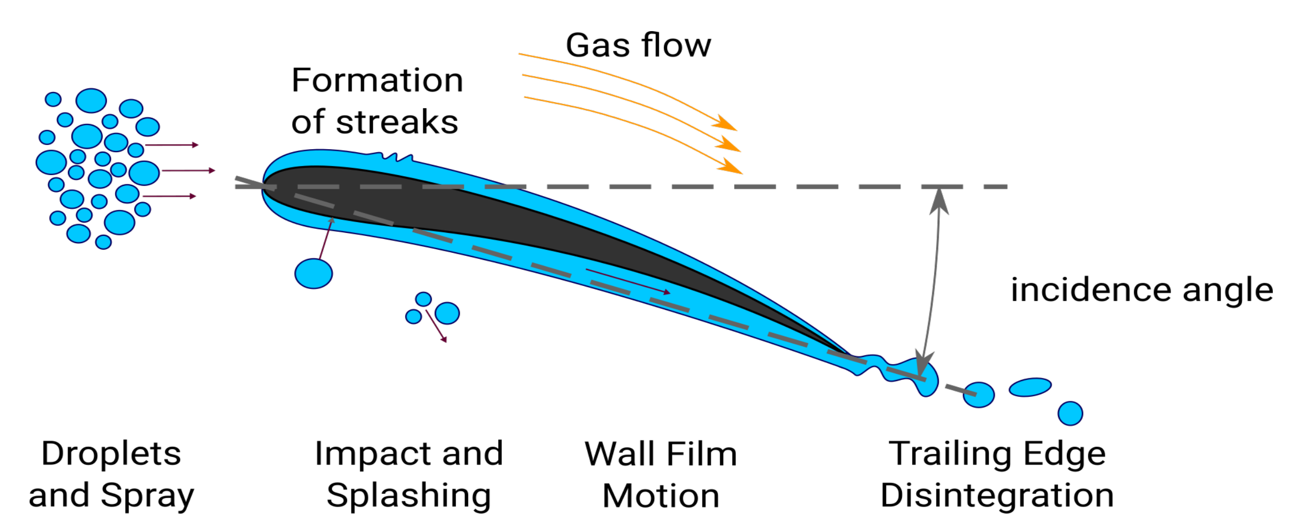
Two-phase flow in gas turbine compressors occurs e.g., at heavy rain flight conditions or in high-fogging applications. The liquid dynamic processes can be categorized into four major processes. All of them are shown in Figure 1. In the following, the processes will shortly be stated, followed by a more detailed description of the processes within each regime. Literature findings will be cited to show the state-of-the-art understanding of the processes and their modeling. In flight conditions, as well as in high-fogging in stationary gas turbines, many polydisperse droplets are present, with diameter distributions in the range of 10 to $200\mathsf{\mu }\mathrm{m}$ [1]. The first process accounts for single droplet interaction with the air flow and the influence of polydisperse spray. As soon as the droplets enter the compressor, interactions with the compressor parts are inevitable, where mainly the compressor blades will be hit by droplets as they are redirecting the flow. This curvature of the streamlines cannot be followed by droplets of all size due to inertia effects and thus droplets impact onto the compressor blade surface. Depending on the incidence angle $\alpha$, impact is possible on the pressure and the suction side. The question arises whether the droplet stays attached onto the surface, or if it is rejected back into the air flow or a combination of both. The subsequent wetting of the compressor blade surface through sticking droplets is another major process, which can be subdivided into wall film motion, wall film breakup and rivulet flow. The last process is the trailing edge disintegration. Driven by the shear of the gas flow, the liquid reaches the trailing edge of the compressor blade and disintegrates into ligaments and droplets. At this point, the processes will start over again, as the outcoming droplets from the first compressor row are penetrating towards the second row and so on.

To highlight the importance of this article for the completeness of understanding all of the processes, their appearance in literature is given in the following. First, droplets and spray are considered. The relative velocity between gas and droplet leads to a deformation of the droplet. If the relative velocity is high, the droplet can break up into smaller fractions. There exist several publications regarding droplets in accelerated air flow, which characterize the outcome. A detailed description of droplet breakup mechanisms can be found in [3]. Droplets with $D\ge 100\mathsf{\mu }\mathrm{m}$ can reach the bag breakup regime, which is experimentally investigated in [4].

Impact on the compressor blade surface is mainly observed for droplets with $D\ge 30\mathsf{\mu }\mathrm{m}$. This can be explained by their relaxation behavior. Analytic estimations considering drag of the droplets show that the limit for perfect relaxation within the characteristic length of a compressor blade lies at $D\approx 25\mathsf{\mu }\mathrm{m}$ [5]. Thus, larger droplets are not able to follow the curved streamlines around the compressor blade and thus might hit the surface. The phenomena of droplet impact onto dry and wetted walls has been investigated by many authors in literature. Although more possible outcomes exist when a droplet hits a wall, for the application of two-phase-flow in gas turbine compressors, only the distinction between deposition and splashing into a number of secondary droplets is of interest. In [6], a splashing criteria is given for droplet impact on dry surfaces and in [7] for wetted surface depending on the liquid film height, respectively. The existence of a liquid film affects not only the splashing limit, but also the splashing outcome. It is possible that more liquid mass is ejected into the air flow than the impacting droplet mass itself. Therefore, the modeling of droplet impact and its outcome play a major role in the prediction of the arising liquid wall film. To gain insight in the deposited liquid mass and the secondary droplet spectrum which is ejected back into the air flow, direct numerical investigations of single droplet impact validated with experimental data were performed in [2,8]. Another approach is to use empirical correlations, as in [6], for single droplet impact on dry walls or in [9] for single droplet impact on shear driven liquid wall films.

If enough liquid mass is deposited on the compressor blade surface, a thin wall film is created. The air flow drives the liquid wall film towards the trailing edge through shear stress. At the pressure side, a closed wavy film runs down the compressor blade. Here, the film is quite stable, as droplet impact occurs continuously over the pressure side. This is mainly due to its concave shape [1]. In contrast, on the suction side, droplet impact is only visible within a short region from the leading edge. As soon as the stabilizing effect of droplet impact ceases, the wall film is sensitive to instabilities. In many cases, the thin wall film breaks up into rivulets. The breakup position, the number of rivulets, as well as their height and width, were experimentally investigated in [1] and an empirical approach to calculate the wall film height is given. Simulations of the liquid wall film under the same conditions using simplified incompressible Navier–Stokes equations were performed in [2]. Simplifications were possible due to the small aspect ratio between film height and blade length. Both methods were capable of reproducing the experimental data qualitatively well. Recently, the breakup of shear driven films and the consecutive movement of rivulets has been analyzed experimentally and analytically in [10].

At the trailing edge, the liquid accumulates and disintegrates periodically. Due to the breakup of the wall film, only separated rivulets reach the trailing edge. In literature, atomization is widely investigated because of its wide field of applicability (combustion, painting, spray cooling, etc). However, research focused mainly on atomization with the use of nozzles or liquid jets and sheets. An overview is given in [11,12,13].One type of nozzle is using a similar method for atomization: prefilm atomizers. Here, the liquid forms a thin film on a wall, driven towards the trailing edge by the concurrent gas flow, where it disintegrates into droplets. In [14], the column-wise disintegration at a prefilmer’s trailing edge is shown and the disintegration of each rivulet is assumed to be independent. Additional information on the influence of ambient pressure and film loading on the ejected droplet spectrum is given in [15]. However, findings from prefilm atomizers cannot directly be adopted to the disintegration at the trailing edge of a compressor blade. This ensues from the geometrical dimensions, as the ratio between prefilmer length and channel height are much smaller compared to gas turbine applications. Therefore, the top wall may influence the boundary layer in prefilm atomizers. First, experimental investigations on trailing edge disintegration in conditions comparable to gas turbines were performed in [16] and continued in [17], with a focus on the droplet size, acceleration and disintegration time. More recently, Refs. [18,19] investigated the effect of the trailing edge size and the angle of attack on the disintegrated droplet characteristics. Ref. [2] investigated the disintegration of a single liquid rivulet at the trailing edge of a thin plate. The goal of the cited work was to gain integral insight in the disintegration process, thus to be able to put up a model for numerical investigations.

This manuscript shall continue the work done in [2]. Instead of using a superhydrophobic surface, a thin acrylic glass (PMMA) plate is used. In addition, the observation area is increased to be able to observe the complete disintegration process, even for larger ligaments. The focus lies on a more detailed description of the disintegration process. This includes the comparison of the whole droplet diameter distribution and their evolution instead of mean values, investigation of ligament length scales at the instance of disintegration and their time scales. In particular, the length scales of ligaments are an interesting feature in gas turbine compressors. It determines if a secondary breakup can take place until the next compressor stage is reached, or if even the ligament will hit the next stage.

2. Materials and Methods

The following experiments are performed in a flow channel with quadratic cross section with an edge length of $80\mathrm{mm}$. The inlet of the flow channel is a nozzle with an area ratio of $31.6$. The nozzle is followed by a section with constant cross section with a length of $6.0\mathrm{m}$. At the end of the flow channel a diffusor with an area ratio of $2.8$ is used to connect the channel to the compressor, which is used in suction mode. The compressor is controlled via the rotational frequency and the maximum volume flow rate can be adjusted by using a throttle valve. Within this experimental campaign, only about $50\%$ of the maximum volume flow rate is used, as it is sufficient to reach the designated velocity range of 10–38 m/s and, therefore, the adjustability of the compressor is higher. The Reynolds number of the air flow $R{e}_G$ is in the range of 12,900–45,600, where

$$R{e}_G=\frac{{\rho }_G{u}_{G}L}{{\mathsf{\mu }}_G}.$$

(1)

In Equation (1), $\rho$ is the density, u the velocity, L is the characteristic length, and $\mathsf{\mu }$ is the dynamic viscosity. The experimental setup parameters are given in

Table 1. Parameters of the experimental test campaign.

Liquid Mass Flow Rate (g/h)	900
Air flow velocity (m/s)	10.5	13.3	15.3	16.7	18.4	19.8	21.4	22.7	23.9
$R{e}_G$	12,930	16,640	18,999	20,737	23,051	25,022	26,809	28,188	29,678
Air flow velocity (m/s)	24.6	26.0	27.2	28.3	29.1	30.3	31.0	31.6	32.7
$R{e}_G$	30,277	32,571	34,374	34,831	35,815	37,625	38,154	38,892	40,246
Air flow velocity (m/s)	33.9	34.7	35.1	36.1	36.8	37.4
$R{e}_G$	41,723	42,326	42,814	44,034	44,888	45,620

.The length of the thin plate $L=20\mathrm{mm}$ is chosen as a characteristic length for the $R{e}_G$ number. The prevailing velocity during the experiment is measured with a Prandtl probe $1.25\mathrm{m}$ downstream from the probe position. Within this velocity range, the three main disintegration regimes can be observed. These are defined analogous to the breakup processes of liquid jets [20]: symmetric and asymmetric Rayleigh breakup and bag breakup.

The test section position is $3.21\mathrm{m}$ from the nozzle exit, which gives an entrance length of $40.1$ hydraulic diameters, after which a fully developed turbulent flow can be assumed [21]. The thin PMMA plate with a length of $L=20\mathrm{mm}$ and a thickness of $t_p=20\mathsf{\mu }\mathrm{m}$ is mounted horizontally in the center of the channel. To ensure that disintegration takes place in the focus plane, the rivulet is guided to the trailing edge in a straight line. This is done by putting a hydrophobic coating on the sides of the PMMA plate, leaving a small gap in the middle for the rivulet with a width of $1\mathrm{mm}$. The apparent contact angle of the two surfaces are ${\theta }_{app}=80.4^{\circ }$ for PMMA and ${\theta }_{app}=105.2^{\circ }$ for the hydrophobic surface. The liquid is supplied through a capillary needle, which enters the flow channel from above and has an inner diameter of $D_{in}=0.6\mathrm{mm}$ and an outer diameter of $D_{out}=0.91\mathrm{mm}$. Its tip is close to the thin plate surface, to ensure that the liquid deposits on the surface without splashing and a less possible disturbance. The liquid mass flow is controlled via a Coriolis mass flow controller (Bronkhorst Deutschland Nord GmbH, 59174 Kamen, Germany).

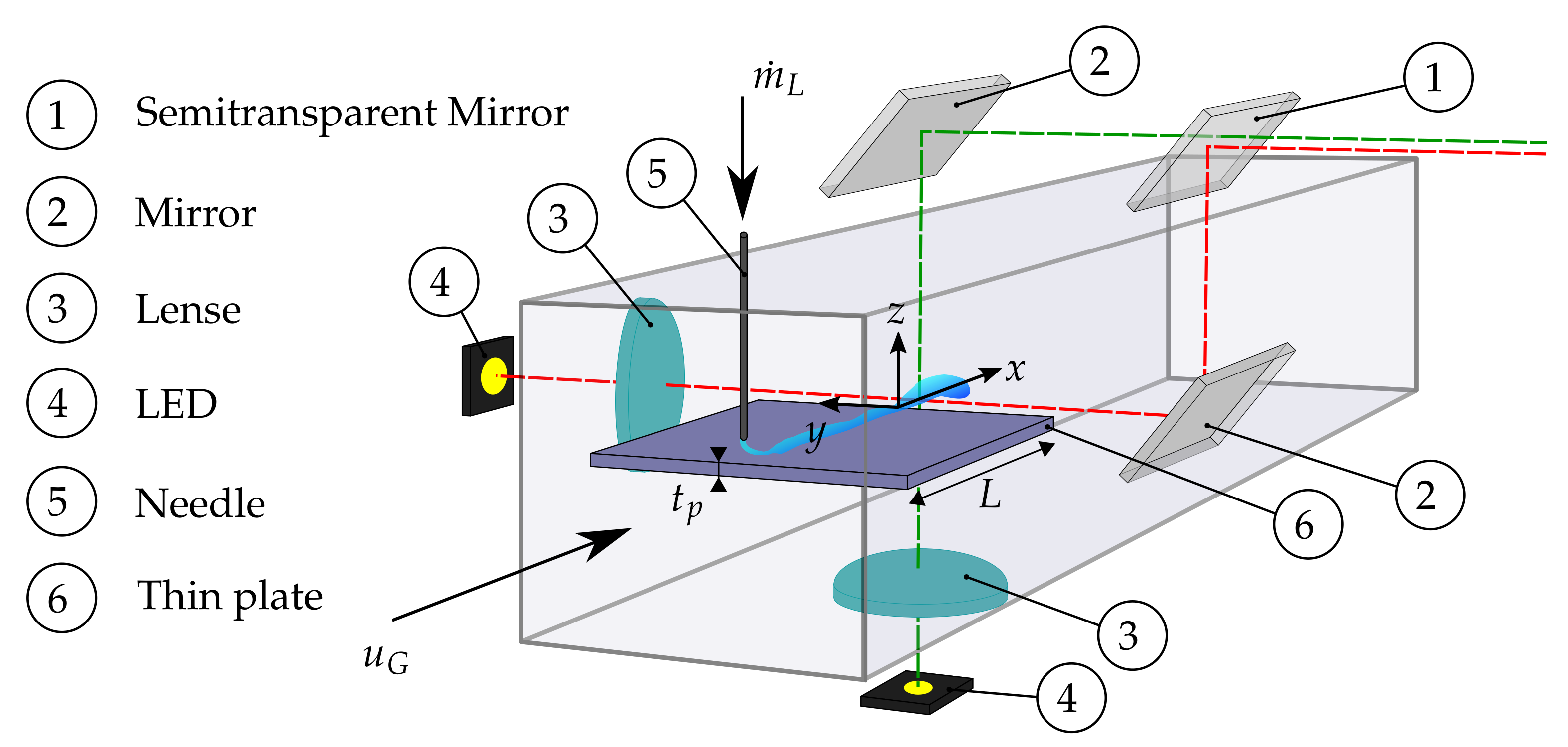
The observation of the disintegration process is done optically, using shadowgraphy. The optical setup is shown in Figure 2, where all parts and the dimensions of the thin plate are labeled and the global coordinate system, with the origin at the trailing edge, is shown. The pictures are lit by a LED on each side and the light is paralellized using plano-convex lenses to gain more brightness and reach uniform background lighting. The top and side view are captured with one camera. Therefore, the optical setup contains two silver-coated mirrors and one semi-transparent mirror. All mirrors are movable with six degrees of freedom to be able to adjust the light path and optimize the captured image. To focus the image on the camera, a lens with a fixed focal length of $f=150\mathrm{mm}$ was used. The aperture was closed as much as possible to gain a large depth of field. This is important, as the disintegration produces ligaments and droplets that fill the whole captured area. A high speed camera (PHOTRON SA1.1) is used at a full resolution of 1024 × 1024 pixels with a maximum frame rate of $5400\mathrm{fps}$, which is needed to capture the high frequencies of the disintegration process. Additionally, when bag breakup occurs, small droplets are catapulted from the lamella at high speeds. To capture this without blur, the shutter speed is set to 1/62,000 s. $8\mathrm{bit}$ greyscale images are used and the scale of the image is 38.9 $\mathsf{\mu }$m pixel for top and side view. The image is split unequally for top and side view with a ratio of 2:3, as the disintegration processes, mainly the bag breakup, takes place over a larger area in the side view than in the top view. The top view is in the upper part of the image, whereas the side view is in the lower part. Together with the scale, this gives a field of view for the top view of 39.8 × 23.9 mm${}^2$ and for the side view of 39.8 × 15.9 mm${}^2$. With these preferences, the high speed camera is able to capture $10,928$ frames, which equals a time interval of about $2\mathrm{s}$. As shown later, the disintegration period decreases with growing gas velocity. This means that, for the same time interval, more disintegrations occur. For statistical measures, it is important to have a sufficiently large number of disintegrated droplets. Therefore, the experimental cases at velocities $v_G\le 15.3\mathrm{m}/\mathrm{s}$ are repeated two or three times to gain a larger database and therefore reduce uncertainty.

In the following, the routine to evaluate the single images will shortly be discussed. The complete evaluation is performed using MATLAB R2020a (The MathWorks Inc., Natick, MA, USA.) As mentioned before, shadowgraphy is used in the experiments. At the beginning of each experiment a background picture is taken, where no liquid is visible. From this picture, the position of the trailing edge can be evaluated. In the first step of the evaluation, each frame is subtracted from the background, which leaves only the liquid structures visible and all background structures and most noise are removed. These differential images are then split into top and side view. The images need to be binarized to evaluate the properties of the visible structures. The threshold to perform the binarization is evaluated separately for the top and side view. To also account for slightly changing brightness intensity between the experiments, the threshold is evaluated for each experiment separately. To set the threshold value, one image of each series containing an exposed droplet is used. The droplet should be large in comparison to its image series. The threshold is then defined as the mean of the inflection points’ gray value of straight lines through the droplet center. An intrinsic routine gathers the properties of the structures in the binarized image, such as area, centroid, eccentricity and the equivalent diameter, which is stored for each image. The equivalent diameter is defined as the diameter of a circle having the same area as the identified liquid structure. A filtering routine removes very small structures, which arise from remaining noise and also identifies the ligament which is connected to the trailing edge. The evaluation of the disintegration period is done semi-automatically, where one period is defined as the disintegration of a connected ligament. 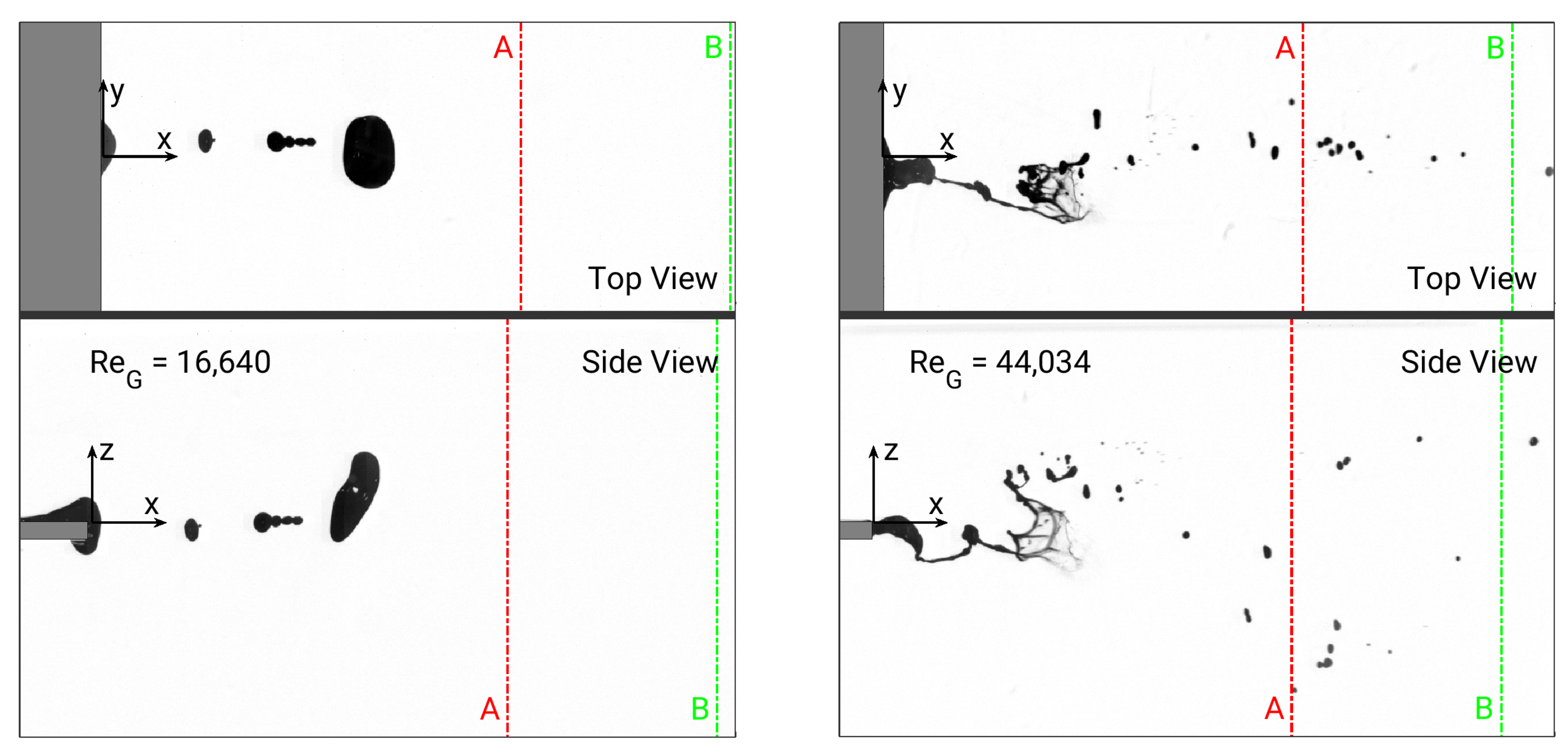Figure 3 shows the disintegration process at two different gas velocities. The corresponding $R{e}_G$ number is given in the image. At low gas velocities, disintegration is easily distinguishable, as the time between two disintegrations is large enough for droplets to be transported out of the observed area. With increasing gas velocities, the process reaches higher frequencies, which leads to overlapping disintegrations, so the droplets of the previous disintegration are not transported out of the observed area, before the following disintegration begins. This makes an automation difficult. Therefore, the routine detects possible disintegration time frames depending on the ligament length touching the trailing edge and the number of droplets close to the trailing edge. The method is implemented conservatively, to assure that all disintegrations are recognized. Excess frames where no disintegration occurs are manually removed. After knowing the disintegration frames, the data for each disintegration can be evaluated in a statistical manner.

Due to the high-speed imaging, several images are taken of the same disintegration. In order to not account for the same droplets multiple times, the droplets are counted at two positions, which are highlighted in Figure 3 with dashed lines. Position A has a distance of 600 pixel ($23.3\mathrm{mm}$) from the trailing edge and position B a distance of 900 pixel ($35.0\mathrm{mm}$), respectively. With the count at the two positions, changes due to secondary breakup can be estimated. The estimation of the droplet parameters is done in parallel for the top and side view and matched together in the end. In this way, not only planar, but spatial information can be evaluated for each droplet. Therefore, the volume can be calculated with higher accuracy and with it derived quantities like the equivalent diameter.

3. Results and Discussion

This section is divided into four parts. The parts describe the different stages on the travel from the rivulet at the trailing edge, over the disintegration process itself to the developed spray and the deviation of the trajectories of the droplets. The first part covers the liquid rivulet and the ligament which is connected to the trailing edge. Second, the disintegration process itself is characterized. Here, the disintegration period and the disintegrated volume are evaluated. Third, the ejected droplets are characterized. The focus lies on the droplet diameter and its distribution depending on the ambient conditions. The last part deals with the droplet trajectories, more precisely with the spreading perpendicular to the air flow direction.

3.1. Rivulet and Ligament Characteristics

In the following, the characteristics of the liquid rivulet and the ligament which still touches the trailing edge are discussed in detail. The evaluated image always shows the trailing edge of the thin plate, which makes the evaluation of rivulet parameters possible. With the two side view, the height and the width of the rivulet can be measured. Both measurements are performed directly at the trailing edge. The third parameter of interest is the length of the ligament, which still touches the trailing edge. The length is defined as the horizontal distance between the trailing edge and the farthest point of the ligament. Over time, all three parameters are fluctuating periodically, which can be explained by mass conservation. The mass flow controller provides a constant mass flow rate, which is transported to the trailing edge. As the disintegration process is discontinuous, but occurs periodically, liquid accumulates at the trailing edge, which leads to an increase of rivulet width and height. At some point, the liquid starts to flow over the trailing edge and a ligament develops. While this ligament is growing, width and height of the rivulet at the trailing edge are already decreasing. As soon as the ligament disintegrates, only a small portion remains at the trailing edge and the cycle starts all over. To compare the three parameters for different $R{e}_G$ numbers, mean values will be calculated. This is done by using arithmetic mean values $\overline{x}$. In addition, the standard deviation S is calculated with

$$S=\sqrt{\frac{1}{N-1}{\sum }_{i=1}^N{(x_i-\overline{x})}^2}.$$

(2)

The number of evaluated data points $x_i$ is N. For the rivulet height and width, all values in each experimental test case are used. For the maximum ligament length, only the values one frame before the ligament disintegrates are used.

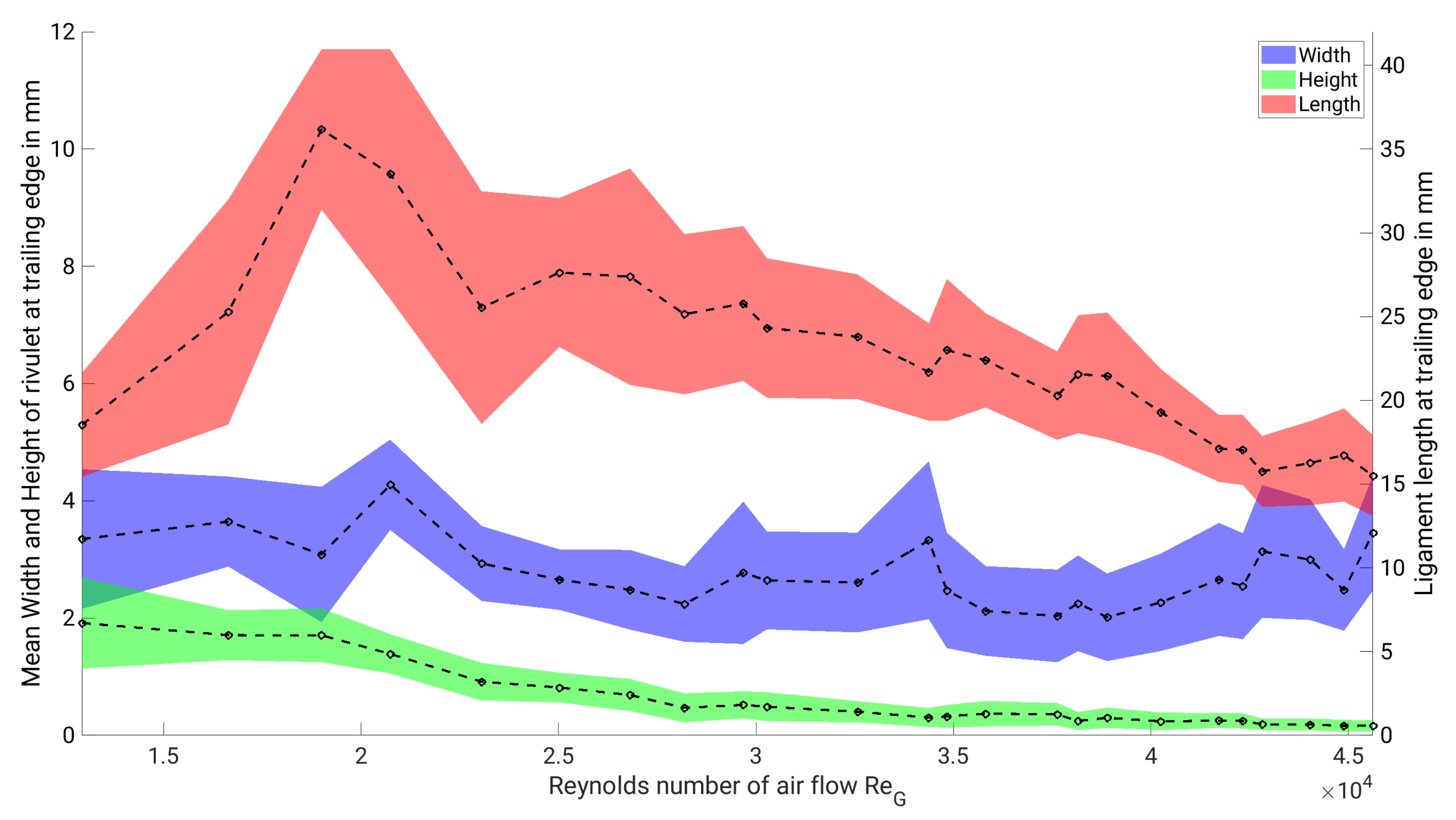
Figure 4 shows the evolution of the three parameters depending on the air flow $R{e}_G$ number. The dashed lines are the mean values, where the dots show the $R{e}_G$ numbers where measurements were taken. The colored area shows the standard deviation S. First, we want to look at the rivulet width (colored in blue). It takes values from $2.0\mathrm{mm}$ at $R{e}_G=38,890$ up to $4.2\mathrm{mm}$ at $R{e}_G=20,740$. However, it is quite constant for a wide range of $R{e}_G$ numbers with a width of about $2.7\mathrm{mm}$. It is also apparent that the standard deviation is nearly independent of the $R{e}_G$ number and has a value of about $S=0.9\mathrm{mm}$. If we now look at the rivulet height, a monotonous decrease is visible. This can be explained by mass conservation. As $R{e}_G$ of the air flow increases, the shear stress at the liquid surface increases. Respectively, the velocity of the rivulet will increase. Thus, with constant width, the height has to reduce to get a smaller cross section to fulfill mass conservation. The standard deviation is also decreasing for larger $R{e}_G$ numbers. Finally, the ligament length $L_{lig}$ at the instance of disintegration will be discussed. It shows an interesting behavior, as it is first strongly increasing with $R{e}_G$ showing a maximum at $R{e}_G=19,000$.

After that, it decreases slowly until it reaches approximately the same value as for low $R{e}_G$ numbers. The standard deviation is large for low $R{e}_G$ numbers with up to $28\%$. However, after the maximum value of $L_{lig}$, the standard deviation is reducing to $17\%$. The non monotonous behavior of $L_{lig}$ can be explained by a change in the disintegration process. At the point of maximum ligament length, the transition from asymmetric Rayleigh breakup towards bag breakup takes place. The air flow velocity is high enough to transport the liquid ligament far downstream, before the Rayleigh instabilities force a breakup of the ligament into droplets. On the other side, the air flow velocity is low enough, so that liquid surface tension is able to keep the ligament together. This is in contrast to high air flow velocities, where liquid bags are also created; however, they are immediately disintegrated into separate droplets.

3.2. Disintegration

Disintegration occurs periodically at the trailing edge. Two main characteristics will be evaluated in the following: the disintegration period and the disintegrated volume. The disintegration period is defined in this context as the time between the beginning of two consecutive disintegrations. The disintegrated volume is the corresponding volume of all droplets that disintegrates from the trailing edge within that time frame. As mentioned above, the definition of a disintegration is easy for low $R{e}_G$ numbers, as the droplets of each disintegration are transported out of the evaluation area, before the next one starts. In the case of overlapping disintegrations, one disintegration is defined as one flapping of the ligament, as can be seen in Figure 3 at $R{e}_G=$44,034.

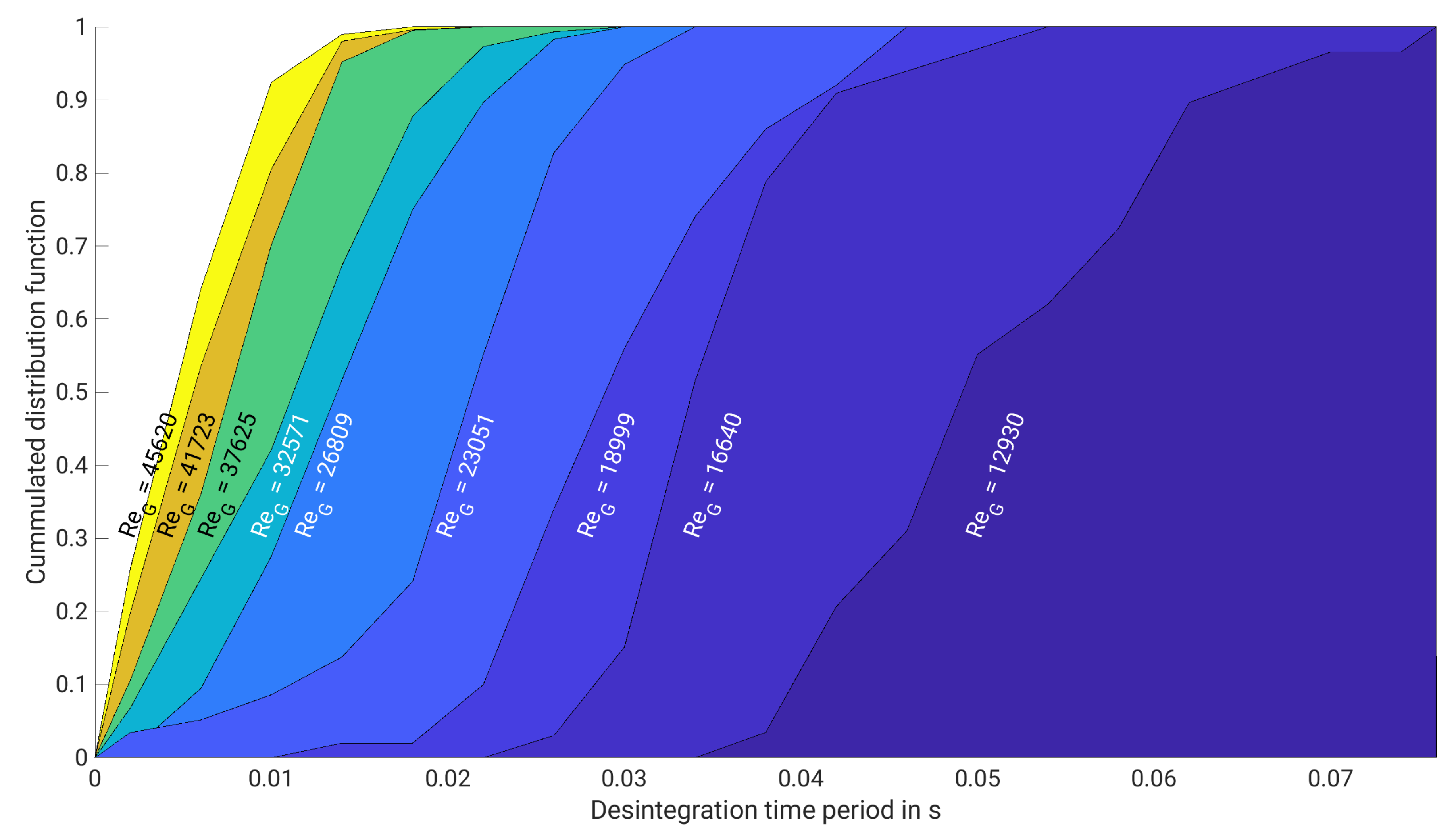
To describe the disintegration period depending on the $R{e}_G$ number, two effects shall be discussed. On one side, the influence on the mean disintegration period and on the other side, the influence on the variation of the disintegration period. In Figure 5, the cumulative distribution function (CDF) of the disintegration time period for different $R{e}_G$ numbers is shown. From the CDF, different results can be seen. The shift of the colored areas from right to left shows that, with increasing $R{e}_G$ number, the average disintegration period tends to smaller values. This shift follows an asymptotic behavior, as the difference is getting smaller for increasing $R{e}_G$ numbers. The averaged disintegration period tends to a finite minimum value of about $0.006\mathrm{s}$.

It needs to be mentioned that the CDF is not shown for every $R{e}_G$ number from the experiments. This is due to the asymptotic behavior. For $R{e}_G>$37,625, the different CDF lie so close together that an optical distinction is no longer possible. From the CDF, statements on the distribution can also be made. The width between the points, where the CDF have the values of 0 and 1, states which disintegration periods were visible in the experiments. The slope at a distinct time value is proportionally linked to the probability of this value. Again, for an increasing $R{e}_G$ number, the width is decreasing and the slopes are increasing. This shows that not only is the variability of disintegration times smaller for higher $R{e}_G$ numbers, but also the probability of disintegration times apart from the mean value.

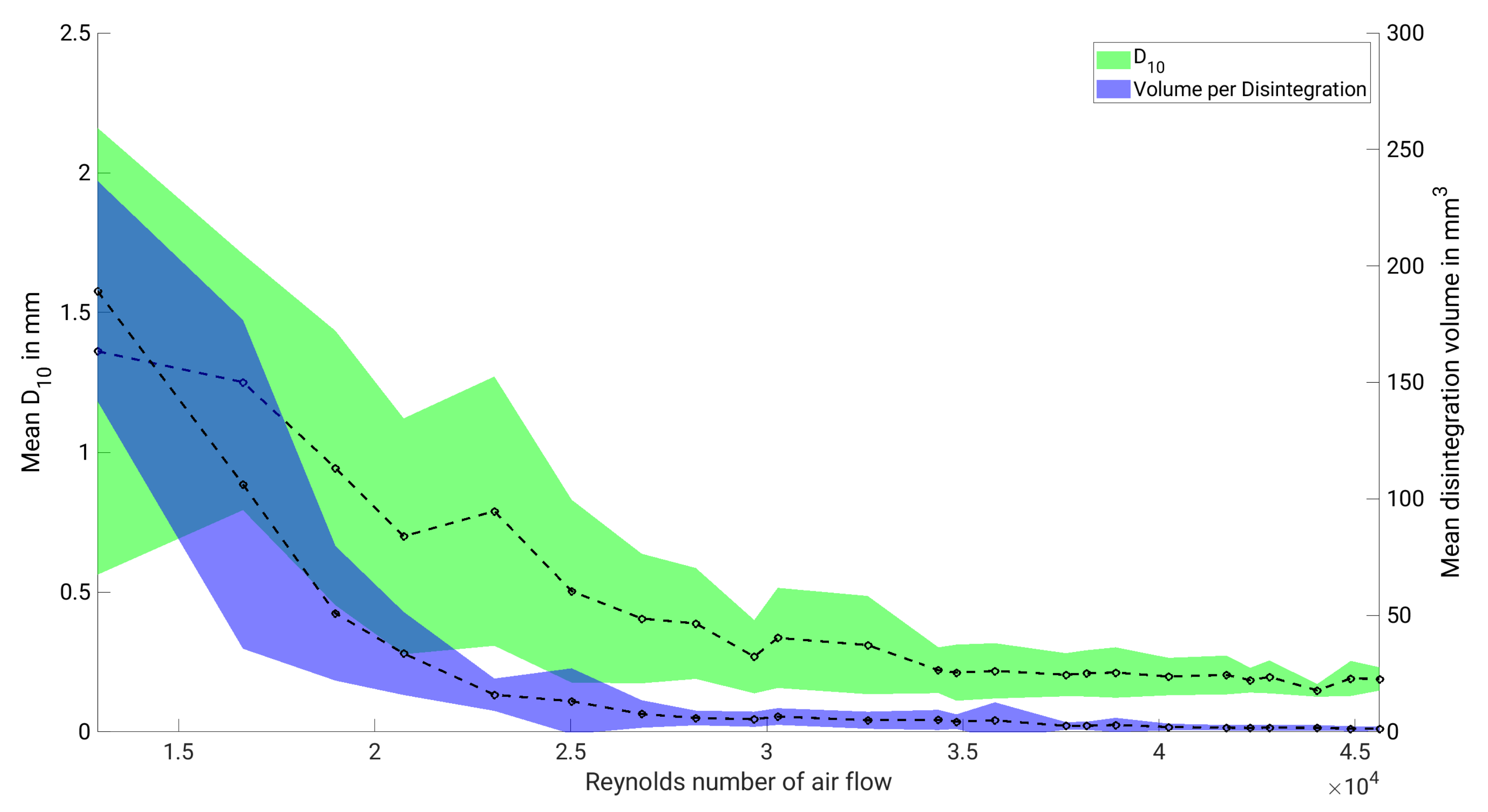
The disintegrated volume is strongly coupled to the disintegration period, as the mass flow rate towards the trailing edge is fixed. Therefore, it is assumed that the disintegrated volume shows the same asymptotic behavior as the disintegration period. This can be seen in Figure 6. The dashed line in the blue area shows the mean disintegration volume. To get the average, the disintegrated volume at every disintegration and the total number of disintegrations observed were evaluated. The blue area shows the standard deviation calculated with Equation (2). The behavior confirms the above stated assumption. With increasing $R{e}_G$ numbers, the disintegration volume decays asymptotically to a value of $1.3{\mathrm{mm}}^3$. The same findings apply for the standard deviation.

3.3. Droplets and Spray

At the instance of disintegration, one ligament contains the whole disintegrated volume for the cases where no bag breakup occurs. With time, this ligament further disintegrates into smaller droplets due to surface tension and shear stress through the outer air flow. If bag breakup occurs, the thin film of the bag ruptures and many small droplets are ejected before the ligament disintegrates from the trailing edge. The resulting spray of droplets will be characterized in the following two ways. First, an integral view by comparing the mean droplet diameter $D_{10}$ will be given. This can be seen in Figure 6. The dashed line corresponding to the green area shows the average $D_{10}$ of all disintegrations within one experiment. The area represents the standard deviation calculated with Equation (2). The overall behavior of $D_{10}$ also follows an asymptotic decrease as has been seen for the disintegration period and volume. It approaches a value of $D_{10}=0.189\mathrm{mm}$. It needs to be mentioned that the averaging only contains droplets that can be seen with the used resolution. Therefore, the diameter of the droplet needs to stretch over at least three pixels to be distinguished from background noise. This corresponds to a diameter of $120\mathsf{\mu }\mathrm{m}$. The ratio between $D_{10}$ at $R{e}_G=$12,930 to the value at $R{e}_G=45,620$ is larger compared to the ratio of the third root of the disintegrated volume at the same $R{e}_G$ numbers. This indicates that the number of droplets ejected at low $R{e}_G$ numbers needs to be smaller than at higher $R{e}_G$ numbers. The large standard deviation at small $R{e}_G$ numbers can be explained with the droplet diameter distribution.

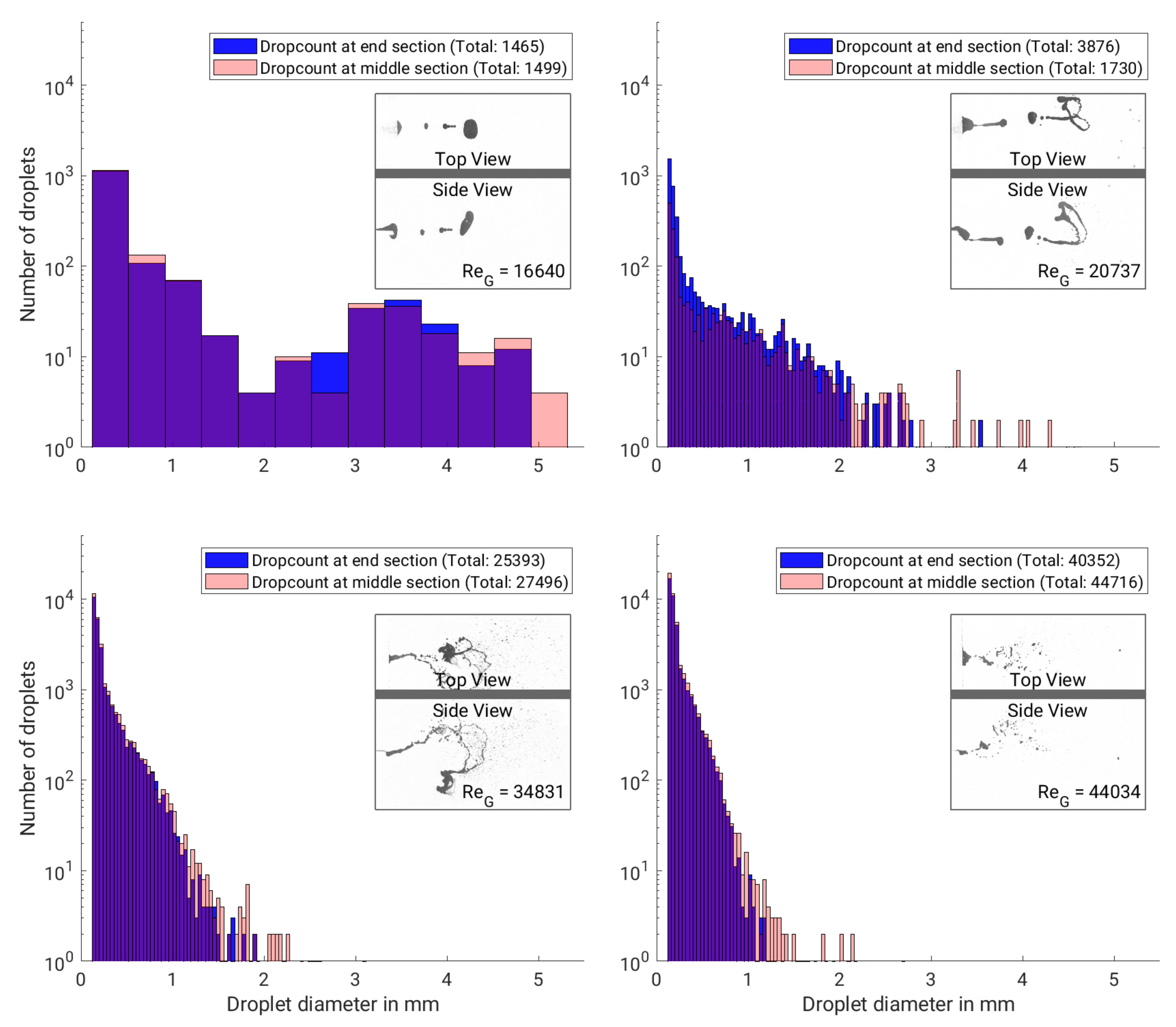
Figure 7 shows histograms and the total number of counted droplets for four $R{e}_G$ numbers. The values are given in the plot. The histogram bin size is adapted to each test case. The $R{e}_G$ numbers were selected to show different observed outcomes within the experiments. To be exact, each plot contains two histograms. One counts the droplets at position A (colored in blue) and the other counts the droplets at position B (colored in red). The positions were described above and are shown in Figure 3. The idea of these two counting positions is to show secondary breakup via a shift of the histogram. Every histogram plot contains one frame of the corresponding experiment to illustrate the physical behavior. This frame shows the top and side view, both labeled in the picture. First, the histogram plot at $R{e}_G=$16,640 will be discussed. Both histograms resemble a bimodal distribution. This can be explained by the physical behavior of the disintegration process at this $R{e}_G$ number, which can be assigned to symmetric Rayleigh breakup. Before disintegration, the ligament stretches out into the air flow. Most of the liquid is accumulated at the tip of the ligament. The breakup occurs close to the trailing edge and the elongated ligament disintegrates into one large droplet, which develops from the liquid at the tip and several smaller droplets that are formed from the tail. In some cases, the separation of the smaller droplets is not finished when they reach position A, but at position B. This can be seen by the slight shift of the histogram towards smaller diameters. With this shift, a higher total number of counted droplets is expected at the end. However, a discrepancy is observed here, as the total number is slightly higher at position A. A possible explanation is the minimum droplet diameter that can be evaluated. For $R{e}_G=$20,737, the histogram looks quite different. It resembles a log-normal distribution with a peak at small droplet sizes and a nearly monotone negative slope until a diameter of $2.3\mathrm{mm}$. At position A, droplet diameters up to $4\mathrm{mm}$ can be found. The secondary breakup from A to B is visible, as only diameters up to $3.5\mathrm{mm}$ were measured at position B and the bin counts are higher for smaller droplets. These findings match the characteristics of the physical regime, which is the transition region from asymmetric Rayleigh breakup to bag breakup. As can be seen in the image of the experiment, within this regime, the ligament is elongated and bent up or downwards. The ligaments still have a large volume which results in large equivalent diameters if they are not disintegrated before the counting position. From the curved ligament, a bag can also develop, which then disintegrates into very small droplets. However, at these $R{e}_G$ numbers, disintegration is often ongoing at position A, which explains the strong shift in the histogram and the augmentation in the total number of droplets. The cases for $R{e}_G=$34,831 and $R{e}_G=$44,034 are very similar to each other. The log-normal distribution of the histogram is more pronounced as in the case above. This is visible from the linear slope in the semi-logarithmic plot. Secondary breakup happens at both cases, as the histogram at position A shows non-zero counts for larger diameters compared to the histogram at position B. An overall comparison of the four data samples confirms the findings from above: The ejected droplet diameters are decreasing, both average and maximum diameter. In addition, the total number of ejected droplets is increasing with higher $R{e}_G$ numbers. In conclusion, it shall be mentioned that it is very important to match the observed diameter distribution, especially the large diameters. These droplets hold a large part of the total volume compared to their number. These large droplets are also contributing to the erosion at a high extent, due to their elevated inertia. The inertia causes a higher probability to hit a blade surface and a higher energy level at impact. To be able to model the diameter distribution correctly, a large database is needed, which has been the scope of this study.

3.4. Droplet Spreading

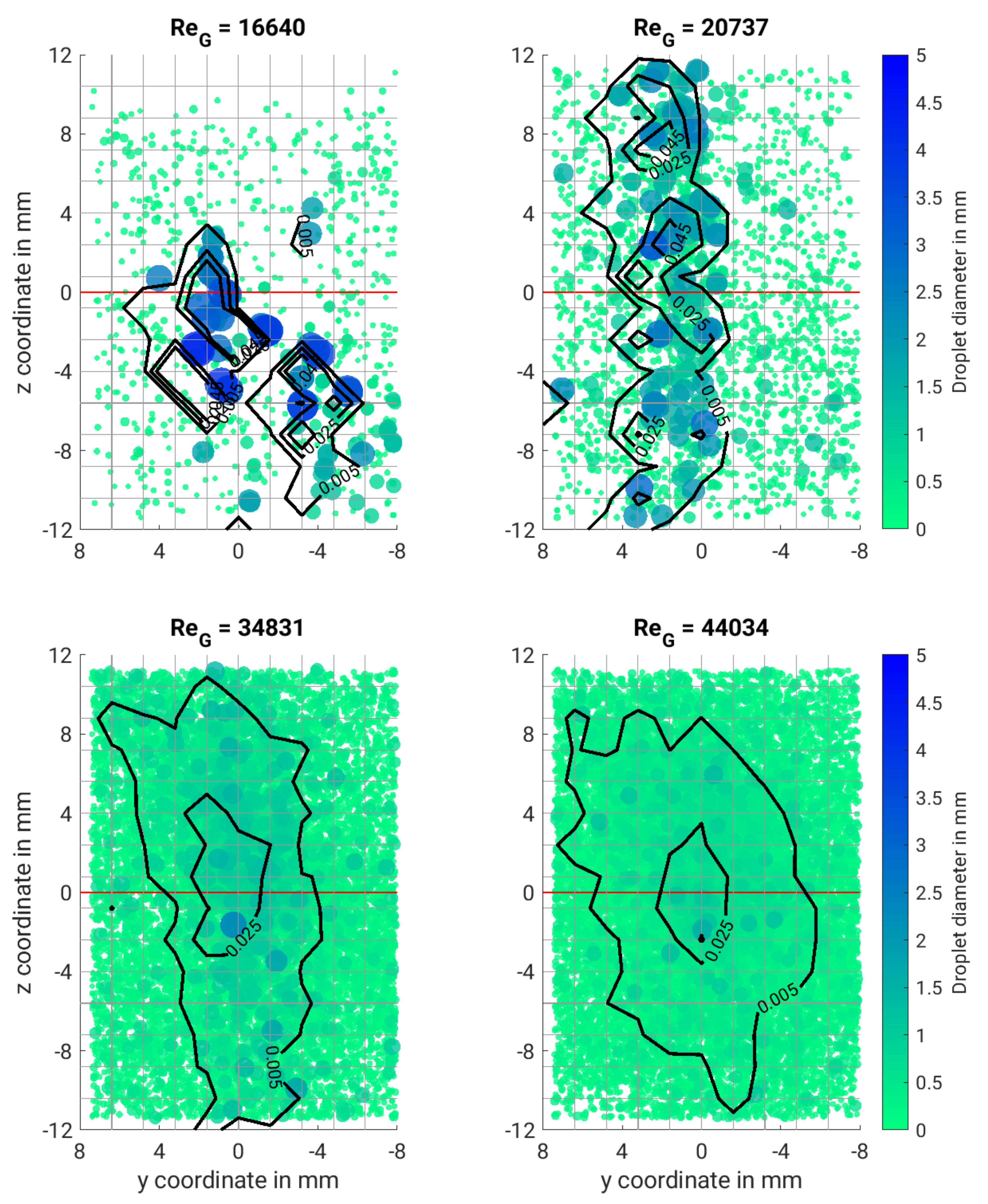
This last section covers the deviation of the disintegrated droplets. Therefore, the location of the droplets at position B is visualized. Figure 8 shows this visualization for the same experimental cases, discussed above. Every droplet that is counted position B is shown as a colored dot. The location is according to the measured value in the experiment. The equivalent diameter of the droplet is visualized with the color and the size of the dot. The position of the trailing edge accords to $z=0$ and the rivulet is placed at $y=0$, which matches the center of the evaluation area. The first observation comparing the plots is again the number of droplets and their spatial distribution. Although the small droplets at $R{e}_G$ = 16,640 are spread widely across the whole area, their number is too small to cover it completely. This is in contrast to the cases with $R{e}_G$ = 34,831 and $R{e}_G$ = 44,034, where the whole area is covered with droplets. However, this mainly arises from the large number of small droplets. Furthermore, it can be seen that the deviation strongly depends on the droplet diameter. Large droplets show less deviation compared to small droplets.

This arises from the fact that the small droplets with the large deviations are mainly ejected within the bag breakup regime. At the instance of bag breakup, the thin film of the bag ruptures and small droplets are ejected radially into the air flow with a high velocity. This ejection velocity distributes them over the whole area. Larger droplets don’t experience this strong acceleration and are therefore not distributed in the same amount. At $R{e}_G$ = 16,640, most large droplets are located at $z\le 0$ mm, which is below the trailing edge. This is due to gravity. At $R{e}_G$ = 20,737, the flapping of the ligament in the $xz$-plane at asymmetric Rayleigh breakup also accelerates the larger droplets in this plane and causes the visible deviation. To further compare the distribution of the droplets quantitatively, the area has been divided into equally sized squares. These are indicated in the plot with the grey grid lines. Within each square, the volume of all corresponding droplets has been cumulated ($V_{sq}$) and normalized by the total volume of all droplets ($V_{total}$). The contour lines represent these normalized values ($V_{sq}/V_{total}$). From the contour lines, it can be derived that, with increasing $R{e}_G$ number, the distribution of the droplet volume across the area at position B gets more continuous. This qualitative statement from optical observation of the contour plots can be confirmed quantitatively—on one hand by the maximum value of $V_{sq}/V_{total}$ and on the other hand by the area that shows a value of $V_{sq}/V_{total}\ge 0.005$. The calculated values are given in

Table 2. Comparison of the cumulated and normalized droplet volume $V_{sq}/V_{total}$ at position B.

${\mathit{Re}}_{\mathit{G}}$	$\mathit{max}({\mathit{V}}_{\mathit{sq}}/{\mathit{V}}_{\mathit{total}})$	${\mathit{V}}_{\mathit{sq}}/{\mathit{V}}_{\mathit{total}}>0.05$
$16,640$	$0.182$	$13.3\%$
$20,737$	$0.082$	$24.0\%$
$34,831$	$0.042$	$37.3\%$
$44,034$	$0.047$	$39.3\%$

. It can be seen that, for higher $R{e}_G$ numbers, the maximum value of $V_{sq}/V_{total}$ decreases and the area where $V_{sq}/V_{total}\ge 0.05$ increases at the same time. Both indicates that the distribution of the droplet volume is more continuous. The contour also shows how the transition from a spotty to a continuous distribution happens. First, the distribution is spreading in the z-direction. This is due to the up and downward flapping of the ligament in the asymmetric Rayleigh breakup. As soon as bag breakup becomes more dominant, the radial spreading of the droplets prevails and the distribution is also widened in the y-direction.

4. Conclusions

The performed experiments extend the database shown in [2]. The integral findings, concerning the mean droplet diameter after disintegration and also the breakup regimes, are in good accordance with [2]. The additional detailed evaluation of the experiments gives the opportunity to model the disintegration process in a more complex manner. In the following, the key findings will be summarized. The rivulet width at the trailing edge is nearly constant for all examined $R{e}_G$ with a value of $2.7\mathrm{mm}$ and a standard deviation $S=0.9\mathrm{mm}$. The height is decreasing monotonously from $1.9\mathrm{mm}$ at $R{e}_G=$12,930 to a minimal value of $0.16\mathrm{mm}$ at $R{e}_G=$45,620. The maximum ligament length measured from the trailing edge first increases until it reaches a maximum at $R{e}_G=$18,999 with $L_{lig}=7.81\mathrm{mm}$. At higher $R{e}_G$, bag break up occurs more often and the mean ligament length decreases. Disintegration period and volume are strongly coupled and show a monotonous asymptotic decrease with $R{e}_G$ towards the minimum disintegration period of $0.006\mathrm{s}$ and disintegration volume of $1.3{\mathrm{mm}}^3$. The observation of the resulting disintegrated spray shows a change of the diameter distribution from a bimodal to a log-normal distribution with the onset of bag breakup. Additionally, the mean diameter is asymptotically decreasing to a minimum value of $D_{10}=0.19\mathrm{mm}$. Droplet spreading lateral to the air flow is strongly coupled to the breakup regime. At the symmetrical Rayleigh breakup regime, mainly the central region behind the trailing edge will be hit. At the asymmetrical Rayleigh breakup regime, the droplets spread vertically. With the onset of bag breakup, the droplets are spread both vertically and horizontally. Additionally, the homogenity of the lateral distribution is increasing with $R{e}_G$. These findings will help to improve simulations of cases where trailing edge disintegration occurs. The future scope will be to further extend the database to cover a larger range of ambient conditions. Particularly interesting will be the dependence on the contact angle and the liquid mass flow rate. In addition, the investigation of higher air flow velocities is considered to see if another breakup regime can be seen, as for jet breakup. With this database, the existing models shall be extended to cope with the above-mentioned requirements.