One of the important elements introduced in the equations of motion is a characterization of sensors and actuators. The selection is based on the assumed choice for the rendezvous mission and improves the accuracy of overall dynamic behavior. The following sections provide a general description of component suites, their models, and validity. We remind the reader that the motivation for component selection is based on the relative effectiveness for the mission at hand, rather than a theoretical optimization evaluation. In particular, cameras are selected to play a primary role in the relative position measurement.
5.1. Sensors
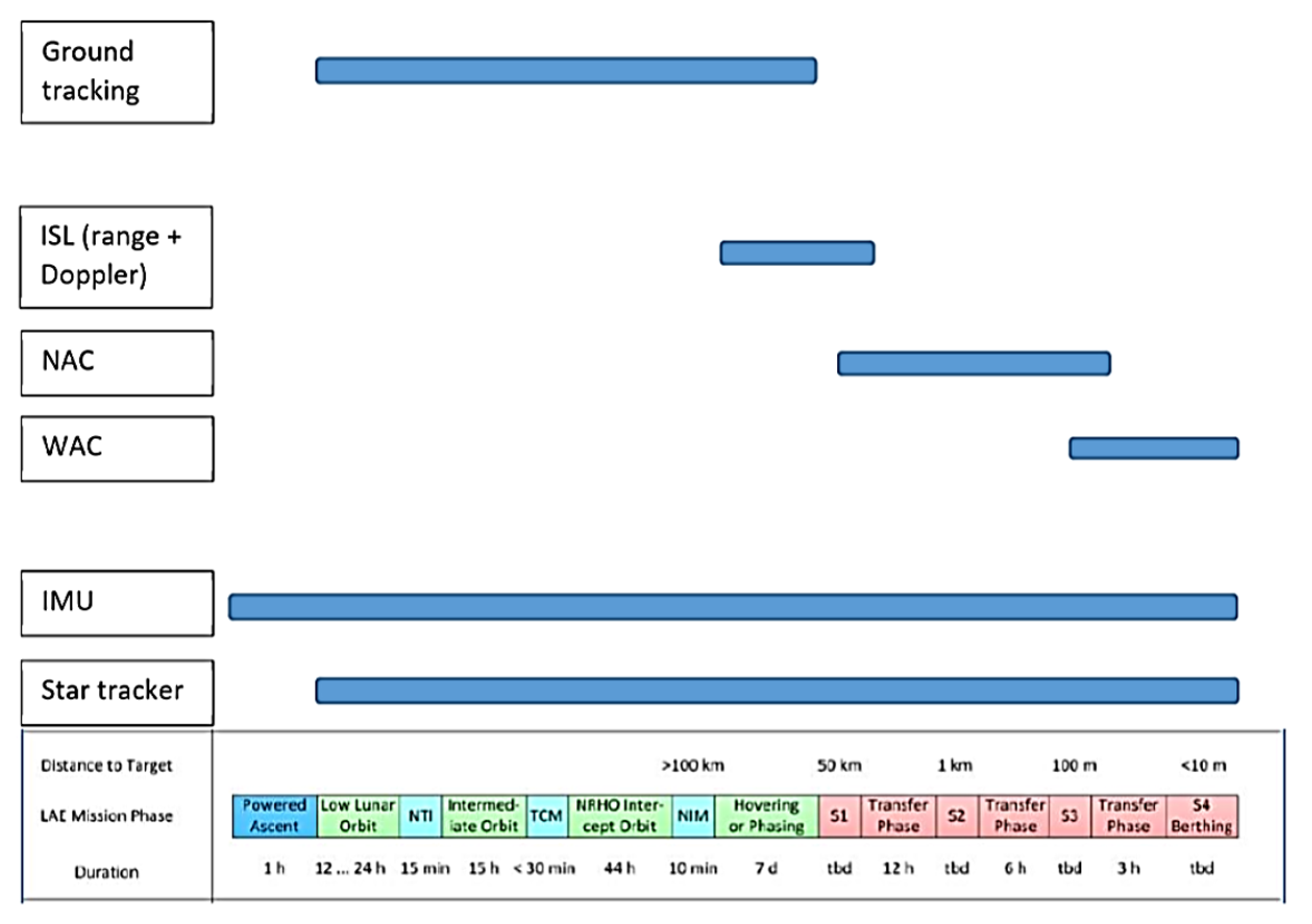
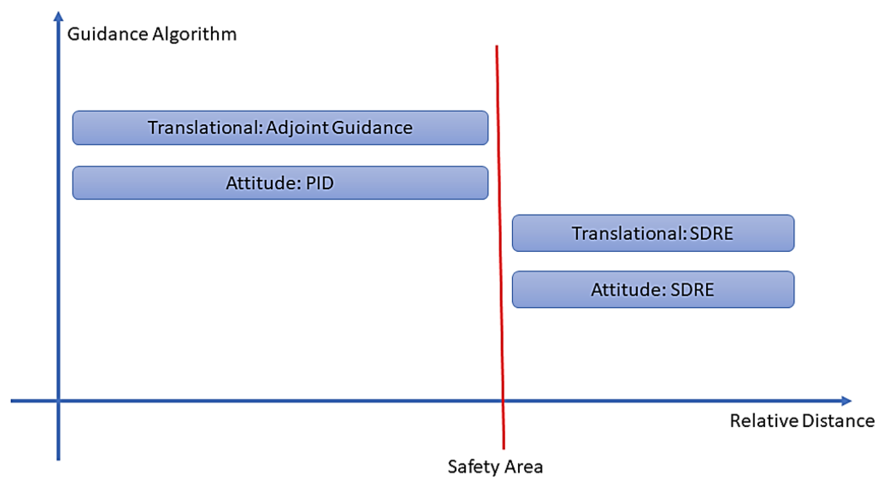
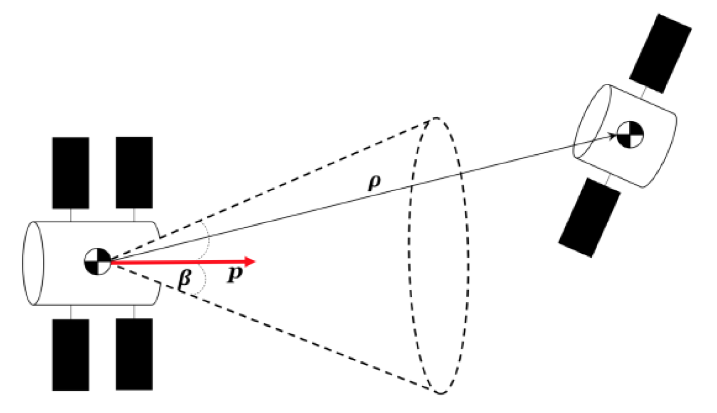
Due to the characteristics of the mission, the set of sensors used by the guidance and control depends on the relative distance between chaser and target, which selects which suite is active at any particular moment. A qualitative representation is shown in
Figure 14.
Of particular interest are:
Inter Satellite Link
Wide Angle Camera
Narrow Angle Camera
ISL, WAC, and NAC were implemented in the model as a single block, with the active sensor selected in relation to the relative distance between chaser and target, with the amount of error committed by the selected sensor’s suite used to define the working ranges of each set-up. The main camera parameters are shown in
Figure 15.
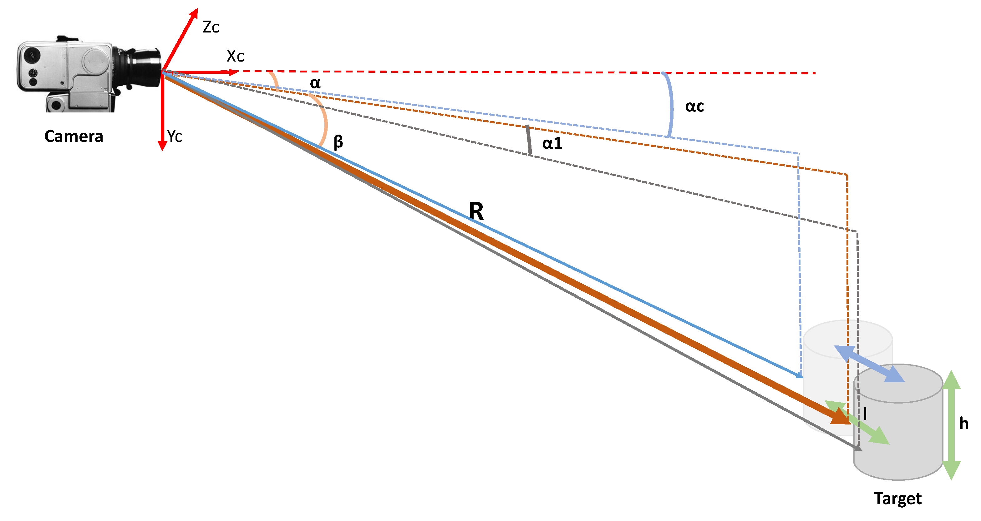
Range estimation using the NAC is computed according to:
The error is a function of the relative distance
R as shown in
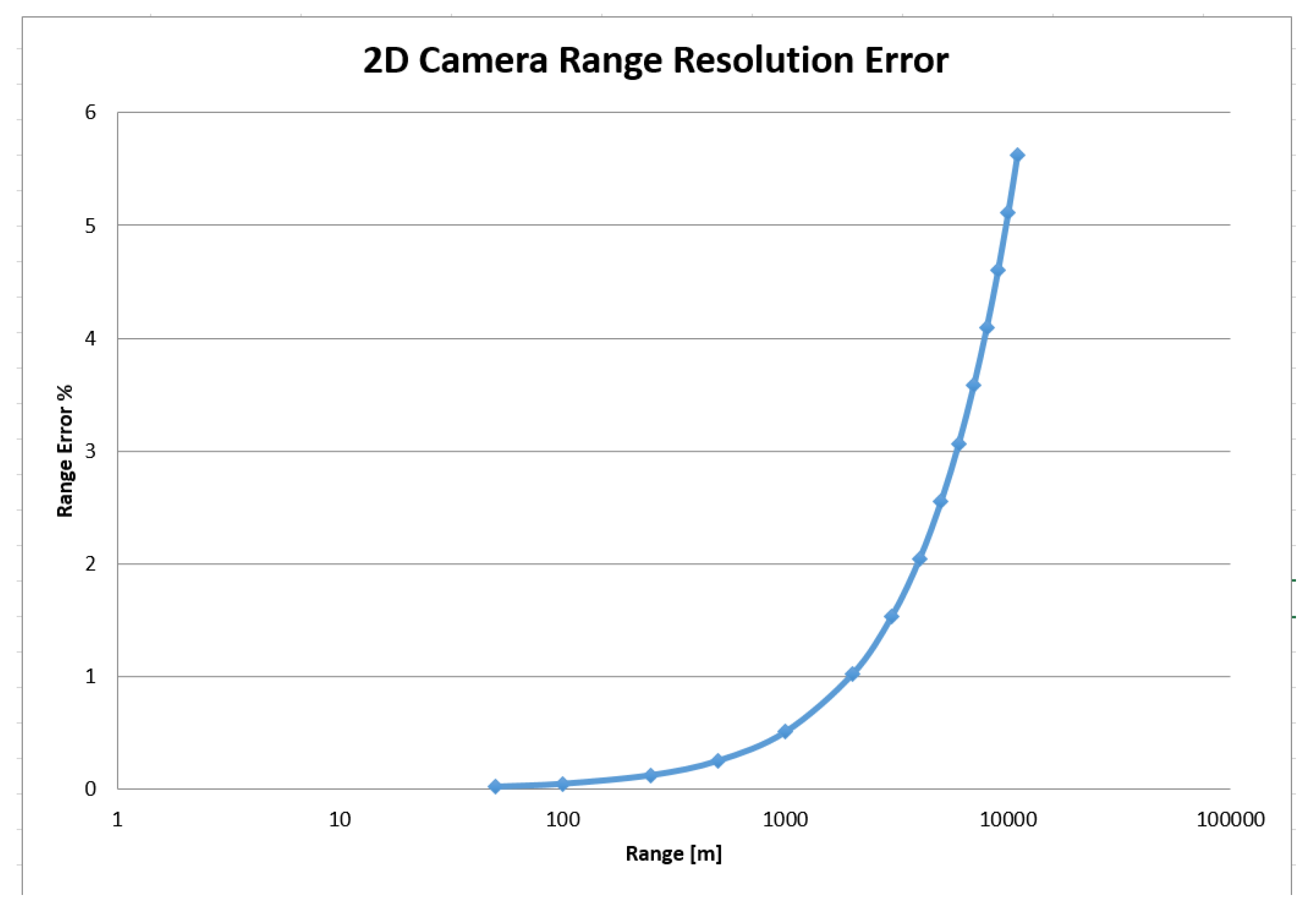
Figure 16.
If the distance is above 10 km, the sensor used to estimate the range is the ISL; in fact, it commits an error in the range estimation equal to
, and, looking at
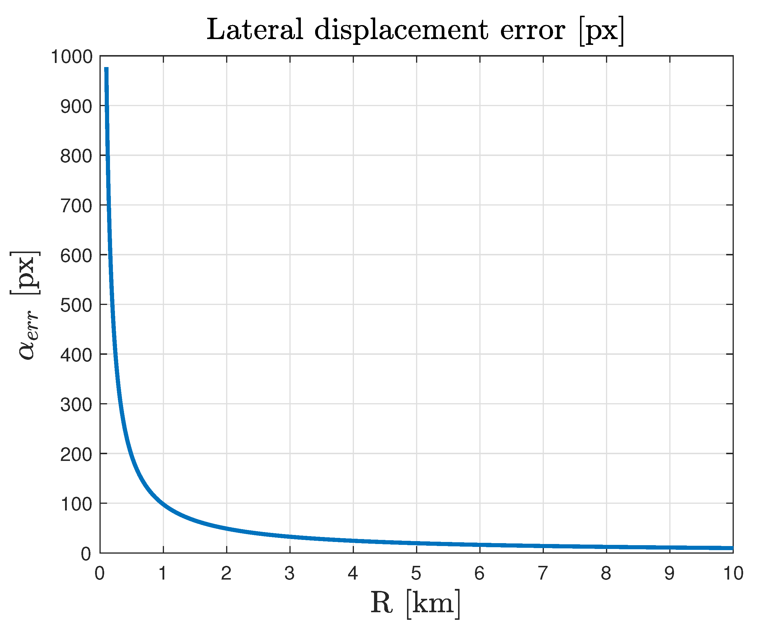
Figure 16, it is possible to notice that the range estimation error produced by the NAC is above
for ranges larger than 6 km. The NAC is also used for the measurement of the lateral displacement (
and
) and an error of
of the target angular visible size is taken into account (about 1–2 px) at large distances.
At medium distances (10 km–1 km), the ISL is deactivated and the range is estimated using the NAC using Equation (21):
where:
l is the target length that is equal to 5 m;
is the measured azimuth angle of the target center of mass, affected by an error of of the target illuminated size.
is the difference between the azimuth of the centre of the illuminated zone and the azimuth of a side of the illuminated zone.
the pixel angular size of the visible Target area.
The lateral displacement is still measured with the NAC and the relative is between 5 and 100 px (
of the target illuminated side). The lateral displacement error is computed using Equation (22), and the trend is reported in
Figure 17.
The angular error
defines the limits between medium distances and short distances; in fact, medium distances are considered those for which
is less than
, but the lateral displacement error, computed with Equation (22), is less than 100 px; as a result, the medium distances are those included in the range 1–10 km:
The short distances are considered those between 1 km and 5 m; here, the sensor used is the WAC and the error on lateral displacement is equal to and the error on R is . At short distances, it is also possible to estimate the relative attitude, with an error of 5 degrees maximum.
The estimation of the translational velocity is based on the differentiation principle and a subsequent Kalman filtering procedure; however, in this work, the entire navigation chain is modeled as in Equation (23):
where
is the relative port-to-port velocity affected by the error,
is the velocity without errors,
is the relative position affected by error,
is the relative position, and
is a white noise.
A similar approach was used to model the angular velocity error, as described in Equation (24)
where
is the relative angular velocity affected by the error,
is the velocity without errors,
is the relative attitude affected by error,
is the relative attitude, and
is a white noise. Both
and
characteristics can be selected by the user.
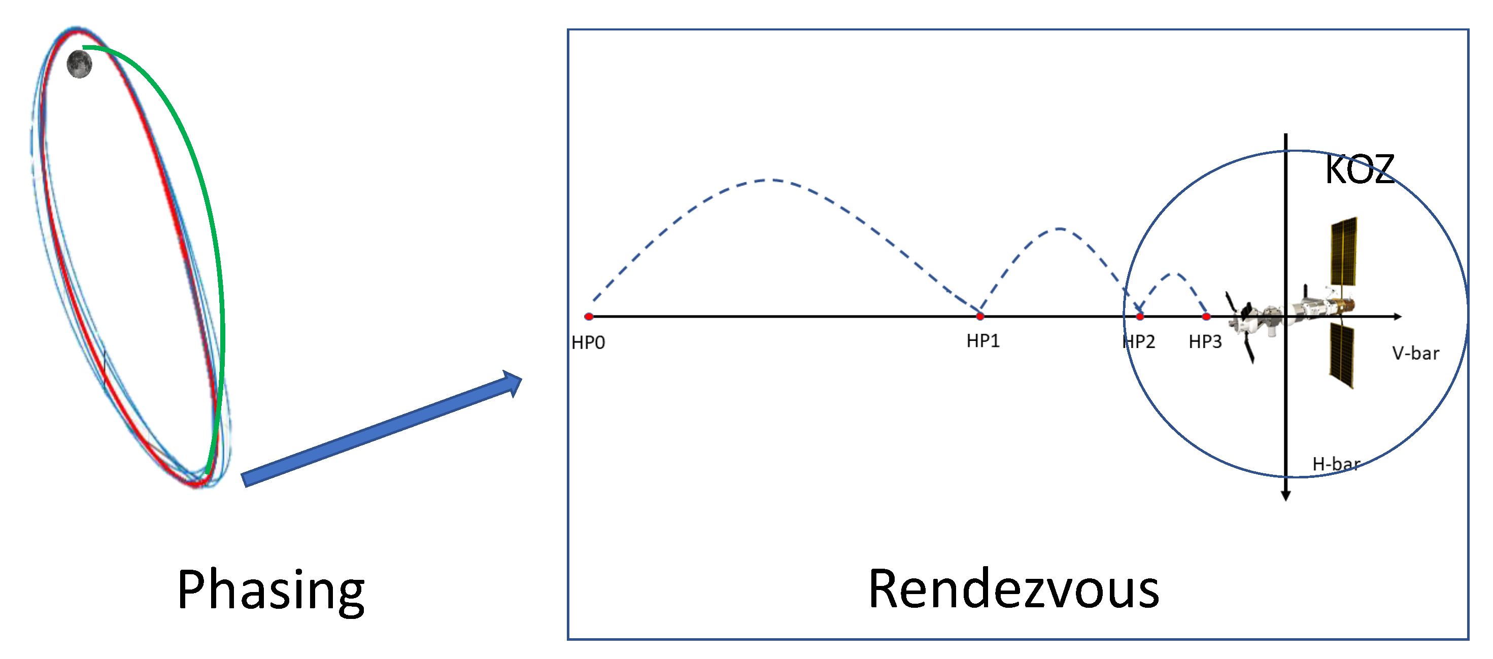
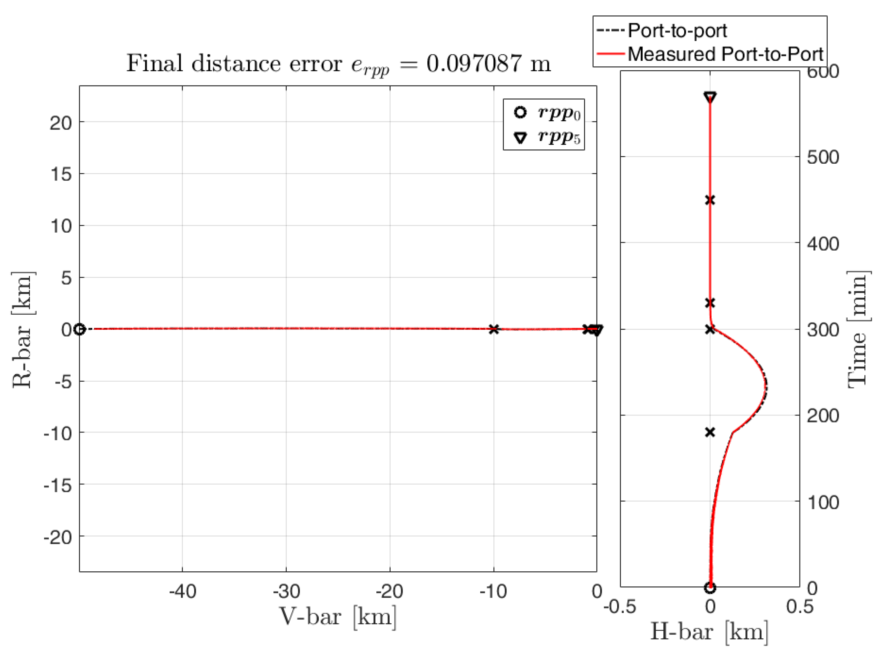
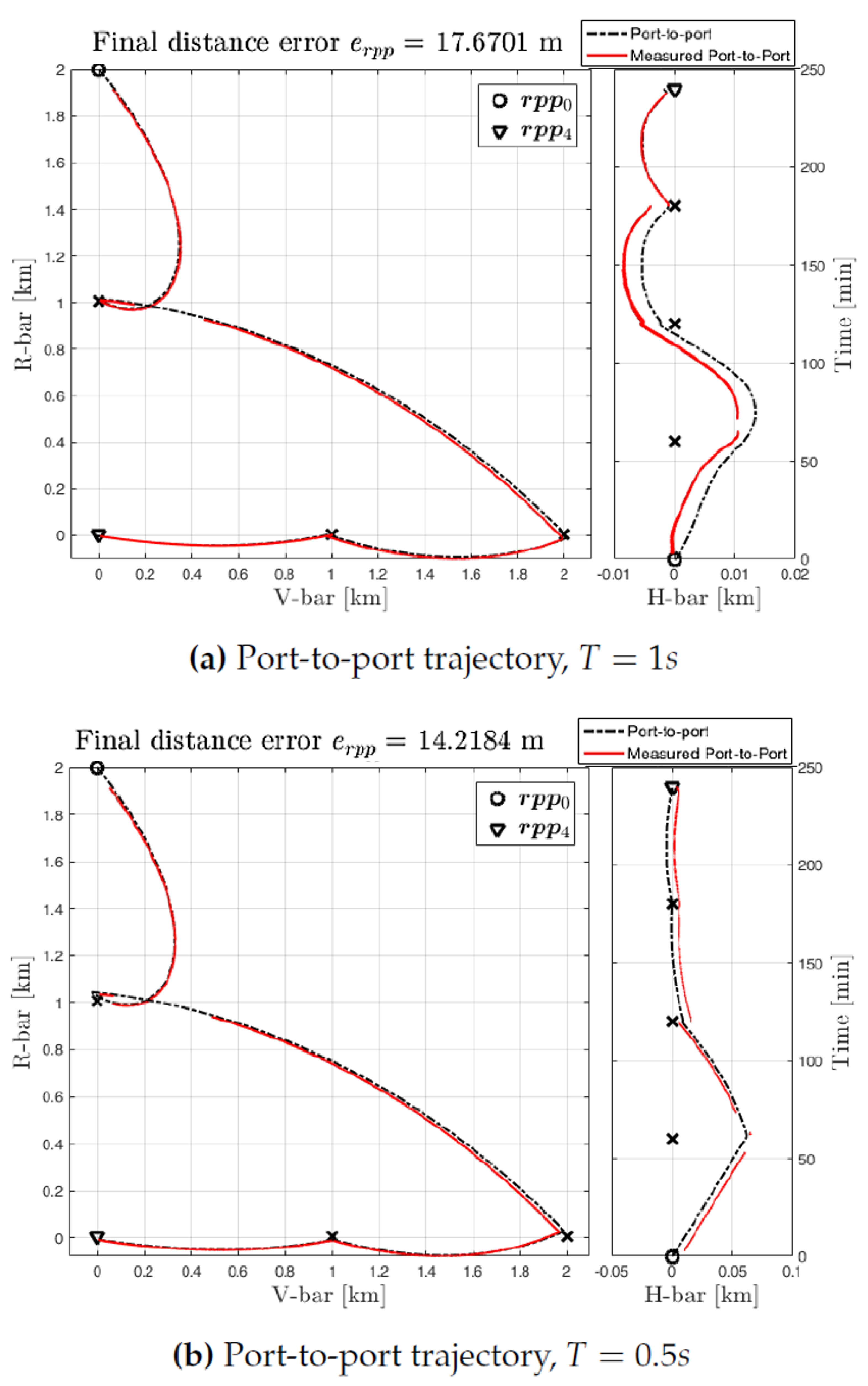
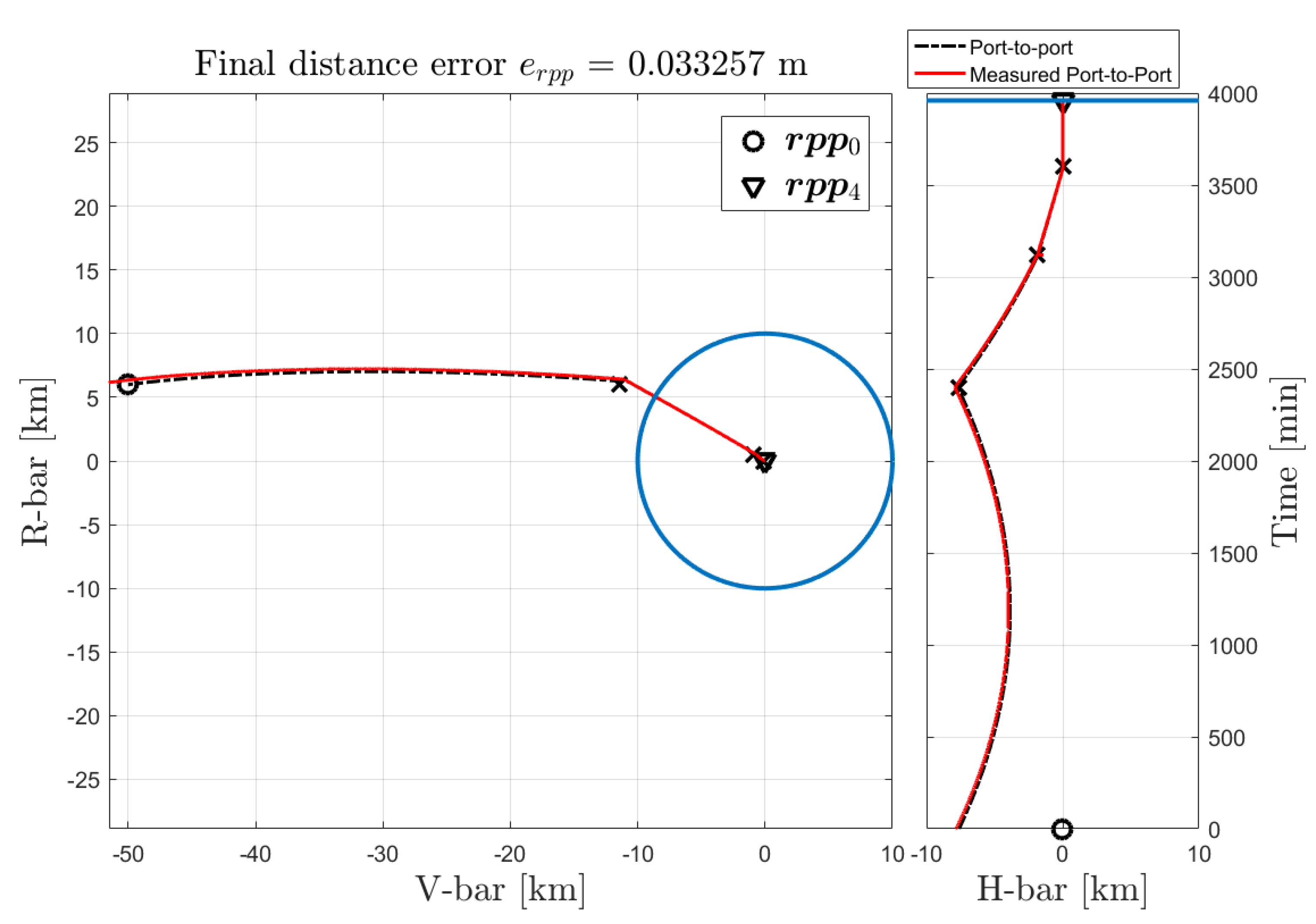
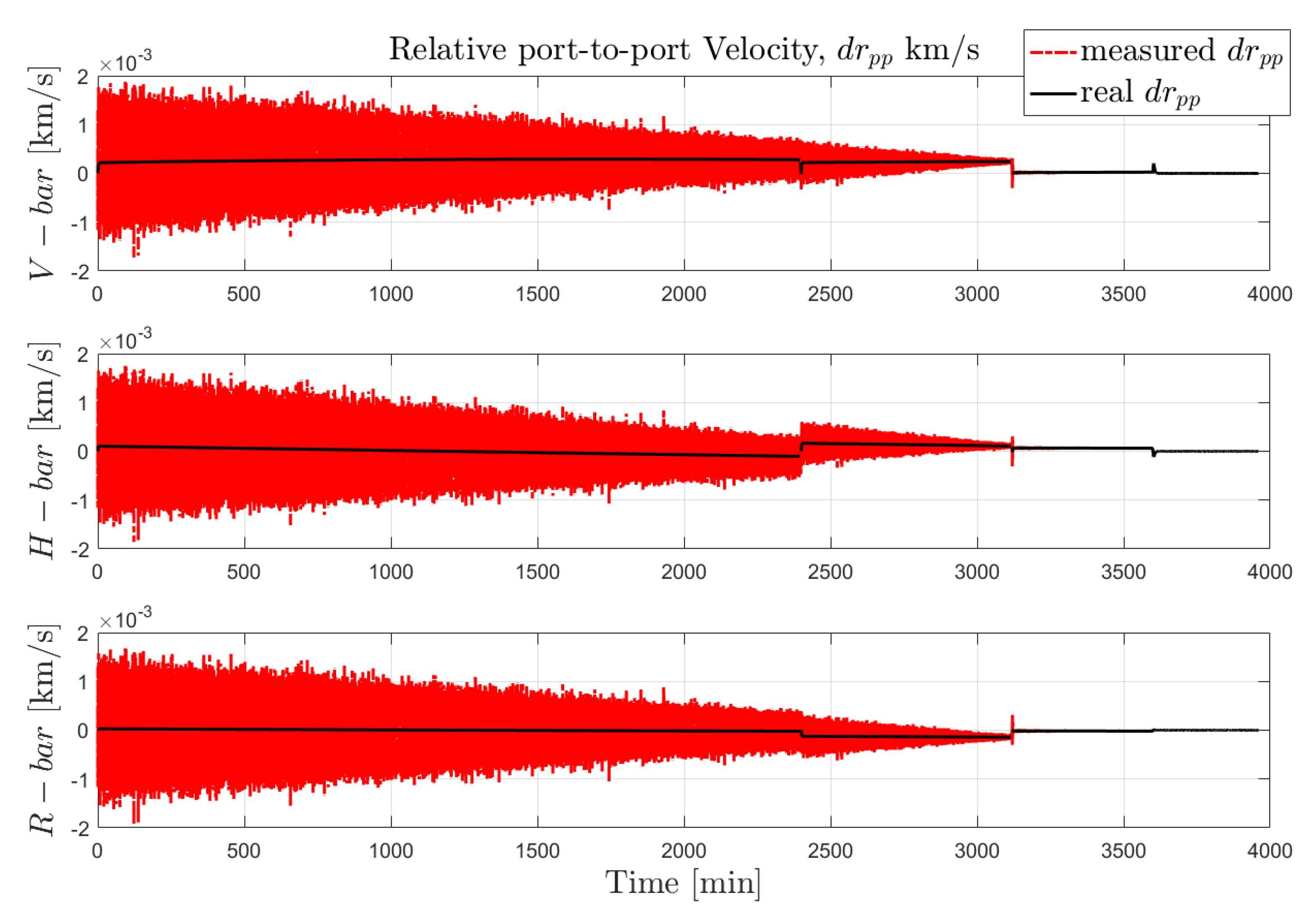
The performance of the sensors with the estimated range measurement is shown by the port-to-port trajectory in
Figure 18 drawn in red, representative of a V-bar approach to the target.
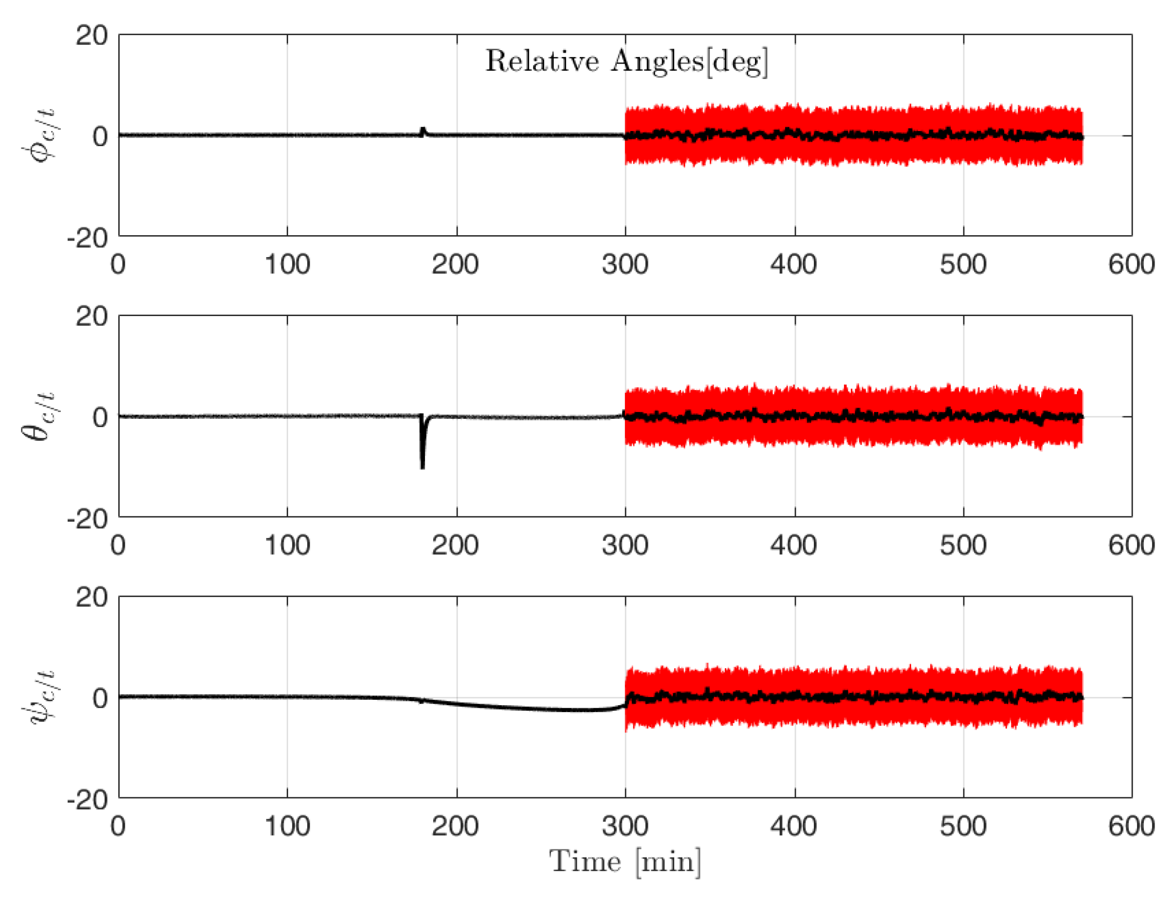
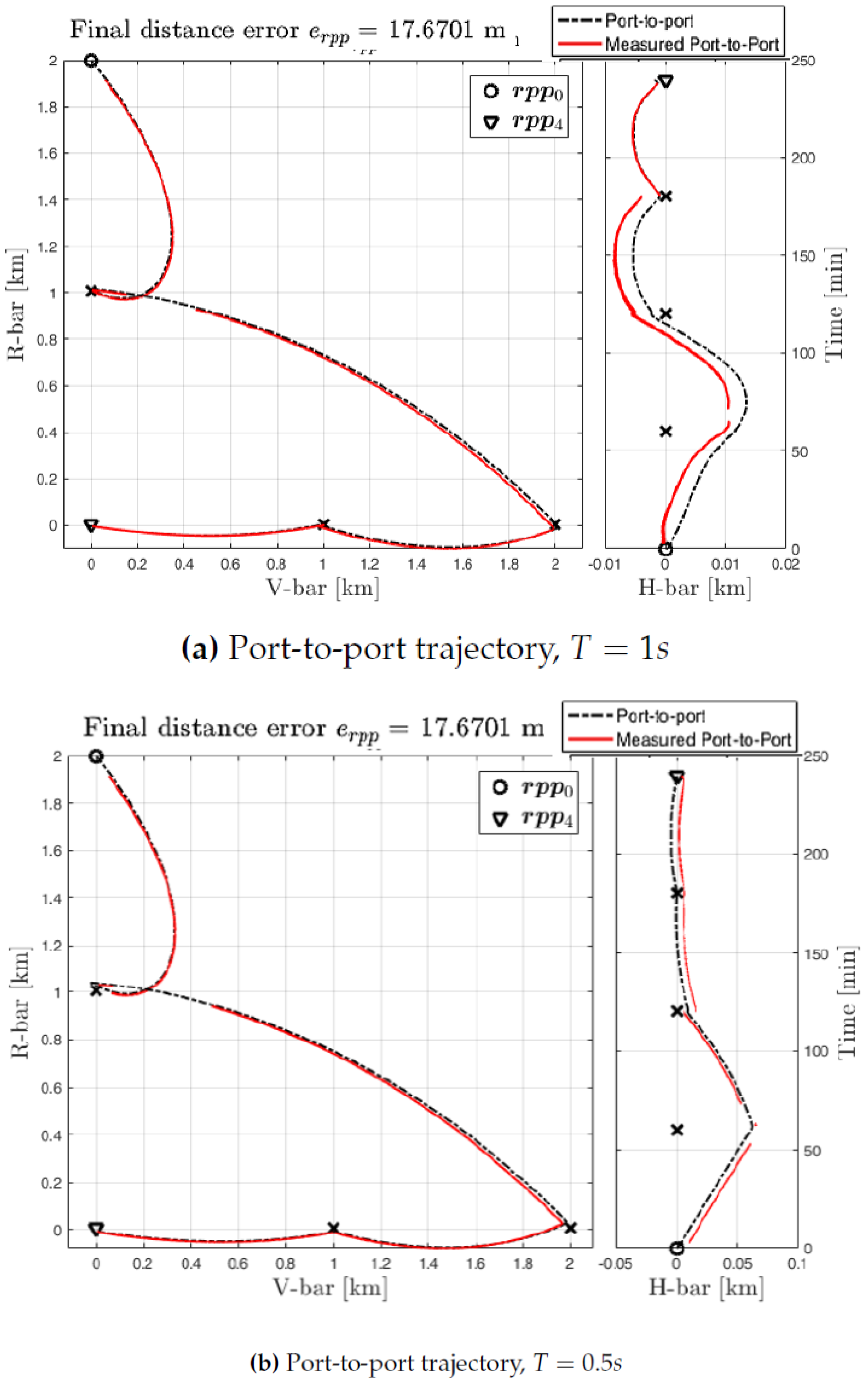
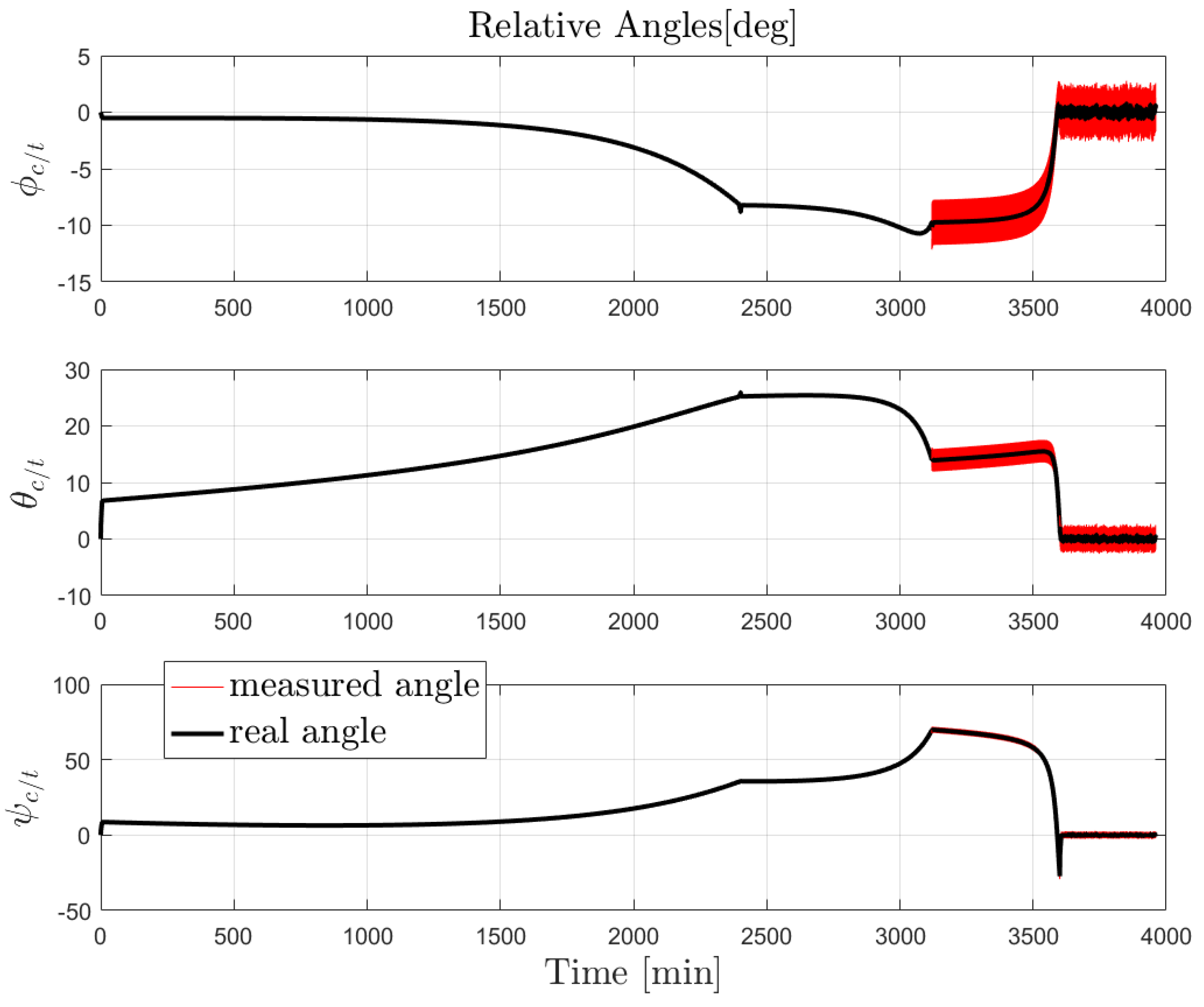
It is important to remark that the range is measured with the camera only when the the target is within the camera field of view; the sensors are initialized at every hold-point and the sensor suite changes only in the hold-points depending on the target-chaser distance at hold-point. The camera is also used to measure the relative attitude for short distances as shown in
Figure 19. The range measurements are always available since we assume the implemented controllers capable of keeping the target within the camera’s FOV.
5.2. Actuators
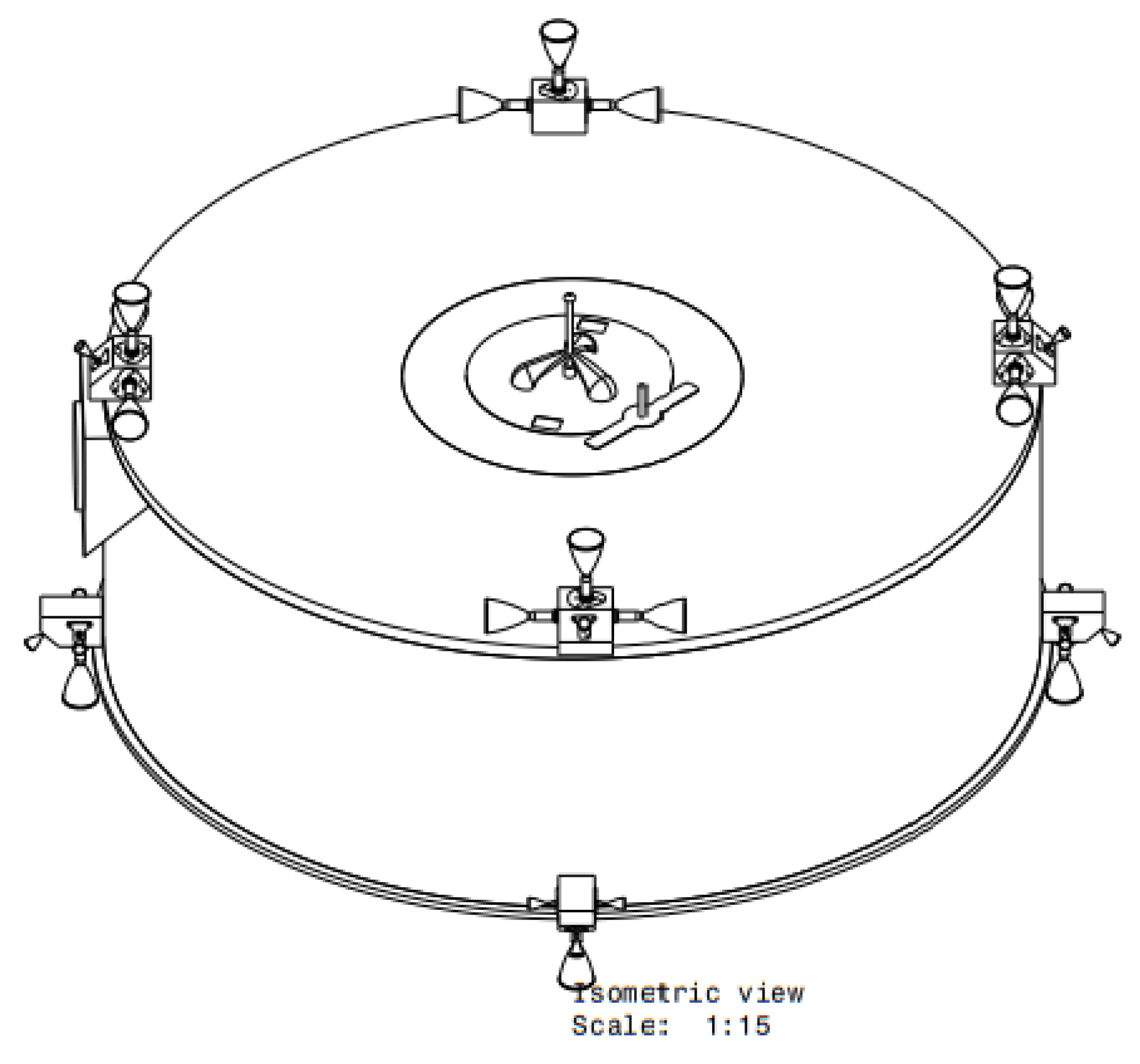
In general, the set of actuators implements the firing command sequences, and allows the vehicle to separate the motion along different axes and the translational motion from the rotational one. With reference to the Heracles mission, the propulsion is implemented by a main engine and 16 RCS-thrusters of 10N each [
11] located on the edges of the chaser vehicle. In this paper, we limit ourselves to describe the model the latter, synthetically shown in
Figure 20 and
Figure 21. The main sources of errors are thrust magnitude errors, thrust direction errors, rise/fall time, and delays.
The sixteen engines magnitude can be modeled as:
where
F is the nominal thrust level at steady state condition,
is the theoretical bit efficiency, and
is the impulse bit efficiency random variation. As said before, in our scenario,
F is equal to 10N.
The theoretical impulse bit efficiency is computed from the empirical formula given by Equation (26), which is based on the duration of the thruster firing command
and the thruster off-time:
and
are expressed in seconds, and
and
are the efficiency factor constants.
According to [
12],
and
can be selected using a PWM approach. The random variation of the impulse bit efficiency
is assumed to be Gaussian with zero mean and the standard deviation
, given by Equation (27).
The misalignment is mainly composed of two contributions: internal and external.
The internal error is due to a misalignment between thrust vector and flange. They are constant over a single thruster firing, but they change randomly from one firing to the next, so the internal uncertainty is assumed to behave as a Gaussian noise. The external errors are due to some misalignment between flange and master reference cube.
The uncertainties remain constant for the entire simulation, but they change from a simulation to the other. As a consequence, the external uncertainty is assumed to behave as a uniformly distributed variable.
In addition to magnitude and direction uncertainty, it is necessary to also take into account the Rise/Fall time behavior [
7]. The thrust is discretized following a PWM logic. The motors have a dynamic and minimum
and
times. The Rise/fall times are taken into account through a filtering operation: the PWM signal will be filter by a 1st or 2nd order filter according to Equations (28) and (29). In the filter equation, we can also take into account a time delay
:
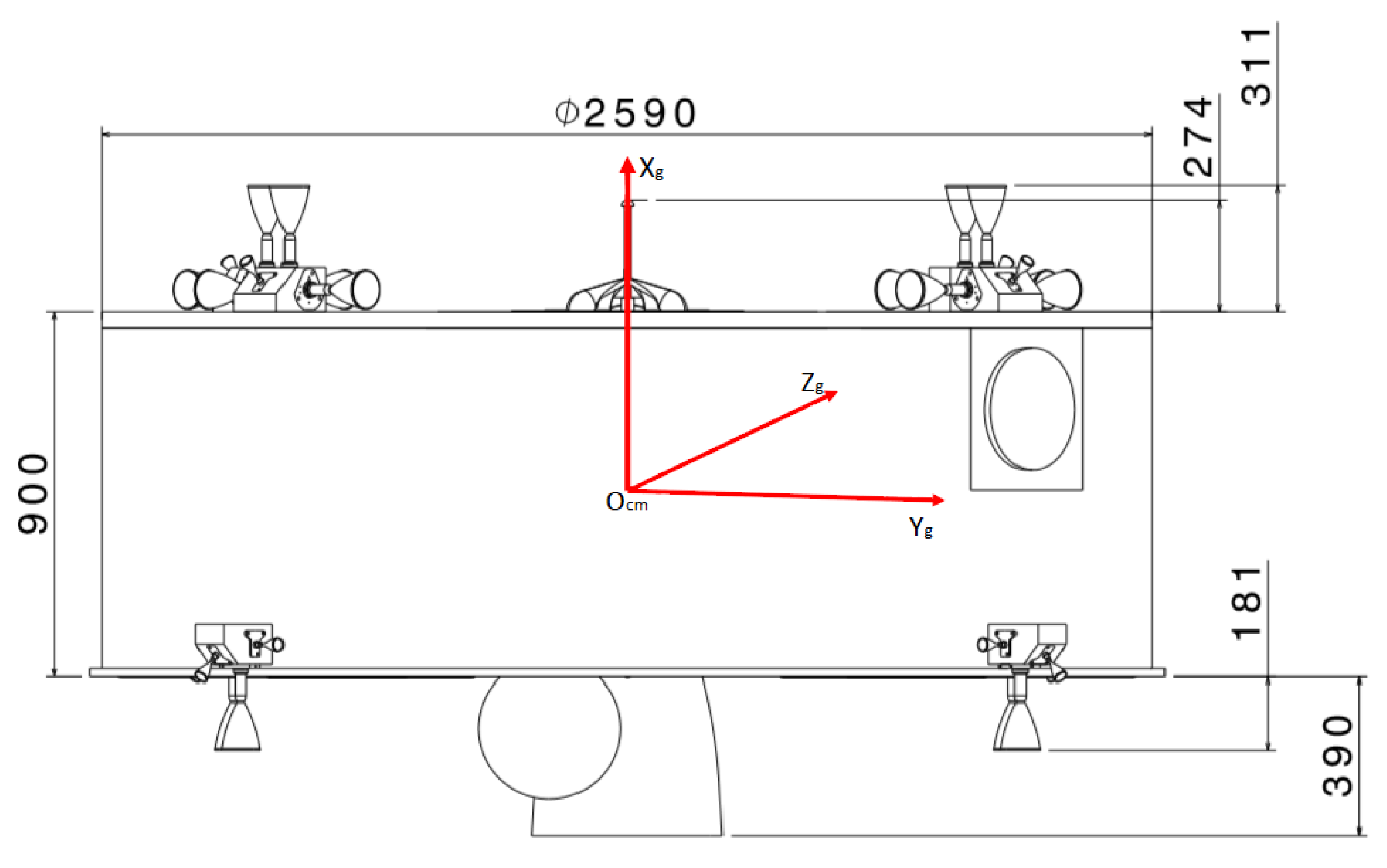
The location of the thrusters depends on the vehicle, its configuration, geometry, and mission. Thus, the contribution that each actuator gives to torques and forces can be computed with respect to the chaser center of mass in the body frame axis, which is the Geometrical frame, defined earlier. Due to the absence of data, the chaser vehicle is considered as a perfect cylinder with uniform density and constant mass; therefore, the body reference system—that coincides with in this case—was located along principal axes of inertia.
The relationship between the thrust of each motor and the torques and forces produced is then computed by projection. Let us define:
, the vector that contains all the thrust provided by the small thrusters:
The 6 × 1 vector of forces and torques, in chaser body frame, is called
, and it is defined as:
The relation between
,
and
is a linear relationship given by Equation (32):
where
is called the 6 × 16 control allocation matrix [
5].
Control allocation is an area with a large amount of literature and many algorithmic techniques, spanning from structural geometry approaches, to several types of optimization methods. Ref. [
13] is especially interesting for our application; in fact, it avoids the use of a PWM module after the control allocation because it computes the optimal combination of duty-cycle to minimize a linear cost function given by:
where
is the vector that contains the duty-cycles; each element of this vector is included between 0 and 1, and
, where
is the maximum thrust supplied by a thruster. It defines the control law in (32).
Another advantage of this technique is that, by minimizing the duty-cycle vector, the fuel-consumption is minimized as well because it is proportional to the summation of all thruster on time. For the reasons briefly explained above, also supported by empirical results, one of the selected control allocation techniques for comparison is the one proposed by [
13]. Clearly, the selection of a specific allocation algorithm also depends on safety factors and software computational power specific for space applications. Therefore, a look-up table approach was also investigated in this study.
The control allocation methods described above are described in detail in Refs. [
13,
14], and the interested reader is referred to them. In the following, we only present rendezvous simulation results as a function of PWM working frequency (1 Hz and 2 Hz, respectively). The optimal control allocation in Equation (33) selects an optimal combination of Pulse Width Modulation duty cycle at each step—in the sense that it minimizes the summation over all duty-cycles and, consequently, the fuel consumption. The optimization method is the interior-point-legacy (default) and the optimization procedure was executed at each step using available routines. The rendezvous maneuver simulation is shown in
Figure 22, indicating better performance with a higher PWM frequency.
In the look-up table algorithm, the thruster modulator is the on-board function that computes parameters for the actuation of the thrusters during a control cycle. The main objective is to compute the percentage of the total duration of the control cycle for which each thruster must be open such that that the average effect of the thrusters over the control cycle results in a force and torque as requested by the controller. The resulting trajectories are shown in
Figure 23, for the same frequency range.
Using the Heracles mission data, a comparison in terms of thrust consumption is shown in
Table 5. The table displays the integral of the acceleration at the thruster during the entire maneuver duration. The “ideal” implies a simulation performed using perfect sensors and actuators, while “non-ideal” indicates results obtained with more accurate models for sensors and actuators as described earlier.


