Article

A Substructure Synthesis Method with Nonlinear ROM Including Geometric Nonlinearities

School of Aeronautics Science and Engineering, Beihang University, Beijing 100191, China
*
Author to whom correspondence should be addressed.
Aerospace 2021, 8(11), 344; https://doi.org/10.3390/aerospace8110344
Submission received: 4 October 2021 / Revised: 6 November 2021 / Accepted: 11 November 2021 / Published: 14 November 2021
(This article belongs to the Section Aeronautics)

Abstract

:
Large flexible aircraft are often accompanied by large deformations during flight leading to obvious geometric nonlinearities in response. Geometric nonlinear dynamic response simulations based on full-order models often carry unbearable computing burden. Meanwhile, geometric nonlinearities are caused by large flexible wings in most cases and the deformation of fuselages is small. Analyzing the whole aircraft as a nonlinear structure will greatly increase the analysis complexity and cost. The analysis of complicated aircraft structures can be more efficient and simplified if subcomponents can be divided and treated. This paper aims to develop a hybrid interface substructure synthesis method by expanding the nonlinear reduced-order model (ROM) with the implicit condensation and expansion (ICE) approach, to estimate the dynamic transient response for aircraft structures including geometric nonlinearities. A small number of linear modes are used to construct a nonlinear ROM for substructures with large deformation, and linear substructures with small deformation can also be assembled comprehensively. The method proposed is compatible with finite element method (FEM), allowing for realistic engineering model analysis. Numerical examples with large flexible aircraft models are calculated to validate the accuracy and efficiency of this method contrasted with nonlinear FEM.

1. Introduction

Geometric nonlinearities must be considered in the design process of modern, high-performance aircraft, especially high-altitude long-endurance (HALE) aircrafts. Because of light-weight design and substantial flexibility, the wings of HALE aircraft always have high slenderness and produce large deformation during flight. Such large deformation leads to vital changes in structural stiffness characteristics and aerodynamic configuration, which obviously affect dynamic response, stability and flight performance of aircraft [1,2,3]. Accurate calculation of structural dynamic response has great significance in the design of high-performance aircrafts [4].
Direct numerical simulation approach of geometric nonlinear dynamic response with physical degrees of freedom (DoFs), such as commercial finite element method (FEM) packages, often holds prohibitive computational burden. Especially for complex aircraft structures, detailed FEM models of structures often tend to possess large numbers of DoFs in order to account for extremely detailed geometric features and material distributions. High computational burden leads to analytical difficulties on aeroelasticity or optimization, etc. Reduced-order model (ROM) is an attractive theory for economical geometric nonlinear dynamic response simulation. Parametric ROM is especially receiving attention, in which the equations of motion are expressed explicitly in the form of ordinary differential equations (ODEs) including polynomial terms of coordinates. These can be directly integrated in the time domain, or be used for further analysis by well-established approaches [5]. Several researches of this approach have been explored in the recent past. Direct and indirect methods are two broad classes of methods for addressing ROM including geometric nonlinearities. In the category of direct methods, knowledge of the dynamic characteristics of the full-order model are required. It is difficult to realize with the complexity of the structures. Indirect methods are non-intrusive and applicable to model establishment with commercial FEM software, which will be more practical. Stiffness coefficients can be obtained from test cases including forces and deformations.
The indirect methods are divided into two categories: the enforced displacement approach and the force-based approach. In the enforced displacement approach, constraint forces are solved after prescribed shape of structures are given [6]. In the force-based approach, corresponding deformations are computed after prescribed forces are applied. Accounting for the effect of foreshortening effects requires additional procedures in these two approaches. Membrane modes or dual modes can be included in structure modeling, and natural frequencies are beyond the bandwidth of interest. Meanwhile, the reduction basis becomes large [7,8]. Modal derivatives (MD) are efficient approaches to enrich the modal basis and have become popular for recovering the foreshortening effects [9]. Hollkamp and Gordon improved the force-based approach to recover the in-plane deformation with the outer-plane deformation which is called the implicit condensation and expansion (ICE) method [10]. Foreshortening effects were captured implicitly in the nonlinear test cases, and high frequency modes were not needed. Response of the axial direction could be simulated in a post-processing step [10,11]. McEwan implemented that approach to conduct dynamic simulations of shells under intense acoustic excitations and received satisfactory accuracy [12,13]. Besides the modal-based reduction techniques described above, the data-based reduction techniques could also be used for ROM construction [14,15]. Cooper and Cestino et al. introduced the ICE method to aeroelastic analysis of large flexible wings coupled with the double lattice method (DLM) and the results presented the important influence of geometric nonlinearities in aircraft structures [16,17]. An et al. considered the follower force effects of aerodynamic loads in static and dynamic aeroelastic response analysis and the simulation results showed satisfied agreement with wind tunnel test results [18,19]. A review of ROM methods for geometric nonlinear structures was presented by Mignolet et al. [20].
Although the ROM method reduces the analysis complexity and cost effectiveness, taking the complex aircraft model as a whole structural model is still unbearable, especially in aeroelastic or optimization analysis where many iterations may be required. The substructure method is widely recognized as an effective method for modeling of structures with a large number of DoFs through dividing structures into simpler substructure components [21]. Compared with the overall modal structure reduction method, the substructure methods can still guarantee low model order and high calculation accuracy. Especially for large flexible aircraft models, the major source of geometric nonlinearities is the wing components. The fuselage and other components of aircraft maintain linearity in flight conditions. Processing all aircraft structures as nonlinear structures will greatly increase the computational complexity and cost. The substructure method considering geometric nonlinear factors in subcomponents should become an important methodology for large flexible aircraft modeling.
Belonging to the fixed interface component mode synthesis (CMS) method, Hurty indicated that the motion of each subcomponent could be expressed by a combination of linear modes, constraint modes and rigid-body modes [22]. Craig and Bampton improved Hurty’s method to integrate constraint modes and rigid-body modes [23]. It is famously known as the C-B method. Rubin combined attachment modes or flexible residual with free interface modes which is also a typical method based on CMS techniques [24]. Craig and Chang developed a free and hybrid interface CMS method by supplemented free interface linear modes [25,26]. Classic substructure methods based on CMS techniques have been proven to be effective in linear structure analysis and there are also many applications of substructure method on concentrated nonlinear problems [27,28,29,30]. With applications in distributed nonlinear problems, Apiwattanalunggran extended the fixed interface CMS method by using fixed interface nonlinear normal modes to analyze structures with weak nonlinearities [31]. Karpel added virtual mass elements to the substructures to simulate the effects of other substructures components [32]. They analyzed the static and dynamic responses of large flexible structures. This method divided the wing component into segments rather than as a whole structure in order to connect with the fuselage, so it was more like a combination of the nonlinear CMS method and the finite segment method. Kantor extended this method and applied it into a simple large flexible aircraft [33]. With strip theory, geometrical nonlinear aeroelastic analysis was implemented. Joannin and Laxalde extended the classic CMS method by nonlinear complex modes for the study of nonlinear and mistuned cyclic structures [34,35]. Kuether presented two modal substructure methods with nonlinear normal modes and a nonlinear reduced-order model under linearization [36]. He also studied a nonlinear substructure method combined ICE method and C-B method with a simple beam model and gave the comparison of calculation results based on back-bone curves [37,38]. Wu et al. developed interface reduction techniques in the C-B method considering geometric nonlinearities and modal derivatives were used for nonlinear displacement recovery [39]. However, existing substructure methods for structure modeling with geometric nonlinear subcomponents is often independently based on the fixed interface substructure techniques. Under the analysis requirement of complex structures, especially aircraft structures, key points of each component, such as wing and fuselage modeling, are different. Development of a hybrid interface substructure technique considering geometric nonlinearities is essential.
This paper aims to develop a nonlinear hybrid interface substructure method in order to solve nonlinear dynamic response analysis problems of large flexible aircraft structures. Complex structure models can be divided into nonlinear components and linear components. The nonlinear components are modeled with ROM by ICE method using selected linear modes as reduced basis vectors in modal space. A series of static test cases are applied to generate nonlinear stiffness coefficients by a regression procedure. Nonlinear stiffness terms of ROM are approximated with polynomials. The linear components are modeled naturally by linear modes. Each component is assembled to satisfy force equilibrium and compatibility by CMS techniques. A set of nonlinear equations of motion can be integrated into simulation dynamic transient responses under various inputs. The application of the method described can be employed with a relatively detailed FEM and largely reduces the computational burden.
The content of this paper is arranged as follows. Nonlinear ROM construction for nonlinear components is presented in Section 2.1. Nonlinear substructure method based on hybrid interface substructure method is introduced in Section 2.2. Numerical examples of a large flexible aircraft are given in Section 3. Considering the characteristics of aircraft, wing sections are modeled as nonlinear components and the fuselage section is simulated as a linear component. The results validate the validity and efficiency contrasted with nonlinear FEM solutions. In Section 4, we finally draw useful conclusions.

2. Theory and Methods

2.1. Nonlinear ROM Method

Construction of ROM considering geometric nonlinearities is illustrated in this section. It can be applied not only to structure modeling with global geometric nonlinearities, but also later for geometric nonlinear component modeling in a substructure method.

2.1.1. Structure Equations

The development of the structural ROM is based on equations derived from a Galerkin approach to solve geometric nonlinear dynamics in a weak form [6]. The equation of motion of the structure may often be given in a dynamic equation as:
  ( F i j S j k ) X k + ρ 0 b i 0 = ρ 0 u ¨ i
where tensor S is the second Piola–Kirchhoff (P-K) stress tensor, tensor F is the deformation gradient tensor, ρ 0 is the mass density of the structure and b 0 is the vector of the body force. X denotes the position vector of the structure in the reference configuration and u i denotes the deformed position vector. With the Galerkin approach, a truncated basis of linear modes Φ = [ Φ 1 , Φ 2 , , Φ n ] are chosen as the basis functions. A quadratic and cubic polynomial form describing the nonlinear relationship and the dynamic equation in terms of the generalized coordinates can be expressed as [18]:
M i j q ¨ j + E i j ( 1 ) q j + E i j l ( 2 ) q j q l + E i j l p ( 3 ) q j q l q p = F i
where M i j are the terms of the reduced mass matrix, F i are the modal components of the external force, q 1 , q 2 , , q n are general modal coordinates, E i j ( 1 ) , E i j l ( 2 ) and E i j l p ( 3 ) are the components of the tensors of the reduced stiffness. Einstein summation convention is applied to the formulation.
When a truncated basis of the linear modes is chosen as the basis functions, M i j and E i j ( 1 ) can be expressed in the formulation as:
{ M i j = M i , i = j M i j = 0 , i j
{ E i j ( 1 ) = E i , i = j E i j ( 1 ) = 0 , i j
where M i represents the modal mass term of the i t h basis function, and E i is the modal stiffness term of the i t h basis function. The formulation of the nonlinear dynamic equations corresponding to the i t h basis function can be written as:
M i q ¨ i + E i q i + E i j l ( 2 ) q j q l + E i j l p ( 3 ) q j q l q p = F i
The nonlinear ROM equations are obtained in modal space with far fewer degrees of freedom than the full-order FE model. Nonlinear modal restoring forces Q ¯ i = E i j l ( 2 ) q j q l + E i j l p ( 3 ) q j q l q p become functions of general modal coordinates q = ( q 1 , q 2 , , q n ) .
In another way, the equations of motion can be discretized by FEM in physical space:
M u ¨ + K u + f N L ( u ) = F
where M is the linear mass matrix and K is the linear stiffness matrix, f N L ( u ) indicates the nonlinear restoring force function, u and F are displacement vector and external force vector in physical space. The geometric nonlinear theory demonstrates that the quadratic and cubic polynomials of displacement are accurate enough to describe the nonlinear restoring force [40]. Introduced linear mode Φ and reduced system by:
u = Φ q
The low-order structure dynamic equations of Equation (6) are in the same formulation as Equation (5). When given specified external forces, the time-dependent modal coordinates can be calculated from Equation (5), and physical displacement vector u is solved by Equation (7).

2.1.2. Regression Analysis of Nonlinear Stiffness Coefficients

An explicit calculation of the nonlinear stiffness is not practical especially for complex FEM models. Regression analysis is used to identify the nonlinear stiffness coefficients E i j l ( 2 ) and E i j l p ( 3 ) , the static formulation of Equation (5) is:
E i j l ( 2 ) q j q l + E i j l p ( 3 ) q j q l q p = F i E i q i
Evidently, if there is a set of specified static loads and corresponding structural deformations, the unknown nonlinear stiffness terms related to the applied loads and the structural displacement resultant can be found by using regression analysis. Corresponding deformation can be calculated by commercial FEM software packages, such as MSC.Nastran [12,13].
Considering that there are NT sets of static test load cases and corresponding deformations, the loads and deformations are transformed into modal space. To solve the unknown nonlinear modal stiffness terms, the left side of Equation (7) can be fitted in a regression progress. The regression problem can be presented as:
{ E i j l ( 2 ) q j 1 q l 1 + E i j l p ( 3 ) q j 1 q l 1 q p 1 = F i 1 E i q i 1 E i j l ( 2 ) q j 2 q l 2 + E i j l p ( 3 ) q j 2 q l 2 q p 2 = F i 2 E i q i 2                                    E i j l ( 2 ) q j N T q l N T + E i j l p ( 3 ) q j N T q l N T q p N T = F i N T E i q i N T
It should be noted that the superscript without bracket denotes the serial number of test cases from 1 to NT instead of the power value.

2.1.3. Strategy for Generating Test Load Cases

Regression analysis is performed using the commercial software package on the actual deformation and load testing after FEM analysis. The accuracy of the nonlinear stiffness coefficients depends directly on the rationality of the selected test load cases, which is related to the success of recovery of the nonlinear structure equations. Two factors are important in generation of test load cases. The first is the spatial distribution of the load over the FEM model. The second is the overall magnitude of the FEM loading [12]. With the absence of a priori information about the exact nature of the nonlinear stiffness coefficients, a sum of a number of weighted mode shapes are often used as test load cases in ROM [12,13,16]. For a given test load cases:
F = r = 1 N R a r K Φ r
Here, F is a vector of discrete loads in physical nodal space, a r are scalar weighting factors for each mode shape and NR is the number of modes selected for test load case generation. The selected test cases cover all the possible nonlinear characteristics of the structure investigated. The desired displacement at the points of interest can be reached by selecting appropriate weighting factors a r . The scalar weighting factors a r can be obtained as:
a r = W c ϕ r ( c )
where W C is the desired transverse displacement at location “C” in the structural model, and ϕ r ( c ) is the transverse displacement of Φ r at location “C”.

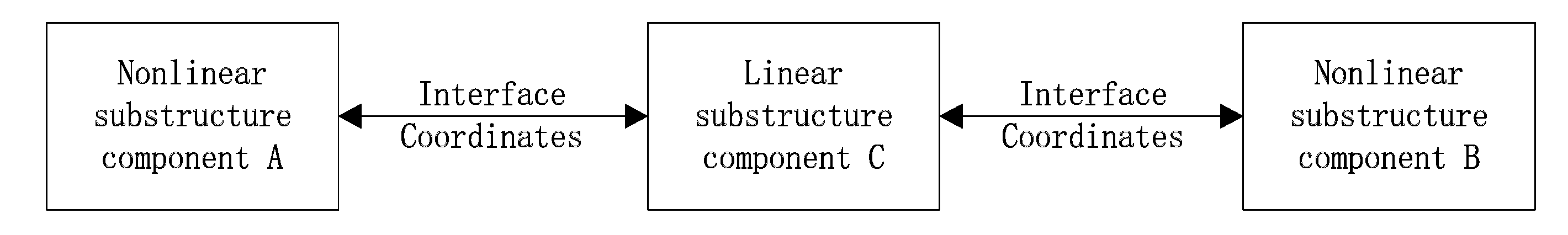
2.2. Nonlinear Substructure Method with ROM

To simulate the dynamic response of complex structure by using the substructure synthesis method, the whole structure should be divided into a limited number of substructures. The substructure synthesis method extended to consider geometric nonlinearities is illustrated in this section. The structure can be divided into nonlinear substructure components with fixed interface and linear substructure components with free interface. Nonlinear components can be modeled by ROM proposed before.

2.2.1. Nonlinear Substructure Component

Considering a nonlinear substructure ( n l = 1 , 2 , , p ) system, each dynamic equation of substructures in physics coordinates can be expressed as:
( m t t m t b m b t m b b ) ( n l ) { u ¨ t u ¨ b } ( n l ) + ( k t t k t b k b t k b b ) ( n l ) { u t u b } ( n l ) + { g t ( u ) g b ( u ) } ( n l ) = { O G b } ( n l ) + { f t f b } ( n l )
Subscript t , b represents interior and boundary coordinates, g ( u ) is the nonlinear function, G b is the boundary load vector and f is the external force vector.
It should be noted that, only the geometrical nonlinear problem is considered here, and the nonlinear problem of interface connection of aircraft structure is not considered. The applied ICE method, g t ( u ) and g b ( u ) can be obtained from regression analysis described before. When given u b ( n l ) = 0 as fixed interface boundary condition, the structure dynamic equation of interior freedoms is:
m t t ( n l ) u t ( n l ) + k t t ( n l ) u t ( n l ) + g t ( u t , u b = 0 ) ( n l ) = 0
Using linear modes to reduce order with u t ( n l ) = Φ t ( n l ) q t ( n l ) , the low order equation is:
M ˜ t ( n l ) q ¨ t ( n l ) + Ω ˜ t ( n l ) q t ( n l ) + g ˜ t ( n l ) ( q t ( n l ) ) = 0
M ˜ t ( n l ) = Φ t ( n l ) T m t t ( n l ) Φ t ( n l ) = d i a g ( M 1 , M 2 , , M n ) ( n l )
Ω ˜ t ( n l ) = Φ t ( n l ) T k t t ( n l ) Φ t ( n l ) = d i a g ( E 1 , E 2 , , E n ) ( n l )
g ˜ t ( n l ) ( q t ( n l ) ) = ( E 1 j l ( 2 ) q j q l + E 1 j l p ( 3 ) q j q l q p , E 2 j l ( 2 ) q j q l + E 2 j l p ( 3 ) q j q l q p , , E n j l ( 2 ) q j q l + E n j l p ( 3 ) q j q l q p ) ( n l ) T
where M i , E i and Φ t represent the modal mass term, modal stiffness term and mode shape matrix corresponding to substructure with fixed interface. Static constraint modes (SCMs) Ψ b are introduced to translate displacement:
{ u t u b } ( n l ) = ( Φ t Ψ b ) ( n l ) { q t u b } ( n l ) = ( Φ t t ψ t b O b t I b b ) ( n l ) { q t u b } ( n l )
The structure dynamic equation can be reformulated as:
( M ~ t M t b M b b M b b ) ( n l ) { q ¨ t u ¨ b } ( n l ) + ( Ω ~ t O O K b b ) ( n l ) { q t u b } ( n l ) + { g ~ t g ~ b } ( n l ) = { O G b } ( n l ) + { f ~ t f ~ b } ( n l )
M b b ( n l ) = ψ t b ( n l ) T ( m t t ( n l ) ψ t b ( n l ) + m t b ( n l ) ) + m b t ( n l ) ψ t b ( n l ) + m b b ( n l ) M t b ( n l ) = Φ t ( n l ) T ( m t ( n l ) ψ t b ( n l ) + m b b ( n l ) ) M b t ( n l ) = M t b ( n l ) T f ˜ t ( n l ) = Φ t t ( n l ) f t ( n l ) f ˜ b ( n l ) = ψ t b ( n l ) f t ( n l ) + f b ( n l )

2.2.2. Linear Substructure Component

Considering a linear substructure ( l = 1 , 2 , , q ) system, each substructure dynamic equation in physics coordinates can be expressed as:
( m t t m t b m b t m b b ) ( l ) { u ¨ t u ¨ b } ( l ) + ( k t t k t b k b t k b b ) ( l ) { u t u b } ( l ) = { O G b } ( l ) + { f t f b } ( l )
According to the basic assumption in the free interface CMS method [25], the displacement of each substructure can be represented by combination of linear modes Φ ( l ) under free-interface boundary and residual modes Ψ d ( l ) as follows:
{ u t u b } ( l ) = ( Φ Ψ d ) ( l ) { q G b } ( l )
Modal coordinates q ( l ) can represent all freedom, and not only interior freedom, because of the free interface boundary condition. The structure dynamic equation can be reformulated as:
( M ˜ O O M b b ) ( l ) { q ¨ G ¨ b } ( l ) + ( Ω ˜ O O K b b ) ( l ) { q G b } ( l ) = { f ˜ t f ˜ b } ( l )
M ˜ ( l ) = Φ ( l ) T m t t ( l ) Φ ( l ) Ω ˜ ( l ) = Φ ( l ) T k t t ( l ) Φ ( l ) M b b ( l ) = Ψ d ( l ) T m b b ( l ) Ψ d ( l ) K b b ( l ) = Ψ d ( l ) T k b b ( l ) Ψ d ( l )

2.2.3. Substructure Synthesis Techniques

For simplicity, it is assumed that the whole structure consists of two nonlinear substructures (Sub-A and Sub-B) components and one linear substructure (Sub-C) component. The connected relationship is shown in Figure 1.
Three components dynamic equations can be presented based on Equations (19) and (21) as:
( M ˜ t M t b M b b M b b ) ( A ) { q ¨ t u ¨ b } ( A ) + ( Ω ˜ t O O K b b ) ( A ) { q t u b } ( A ) + { g ˜ t g ˜ b } ( A ) = { O G b } ( A ) + { f ˜ t f ˜ b } ( A )
( M ˜ t M t b M b b M b b ) ( B ) { q ¨ t u ¨ b } ( B ) + ( Ω ˜ t O O K b b ) ( B ) { q t u b } ( B ) + { g ˜ t g ˜ b } ( B ) = { O G b } ( B ) + { f ˜ t f ˜ b } ( B )
( M ˜ O O M b b ) ( C ) { q ¨ G ¨ b } ( C ) + ( Ω ˜ O O K b b ) ( C ) { q G b } ( C ) = { f ˜ t f ˜ b } ( C )
The compatibility equations of the interface coordinates and forces can be written as follows:
u b ( A ) = u b ( C A ) = B d ( C A ) ( Φ ( C ) q ( C ) + Ψ d ( C ) G b ( C ) )
u b ( B ) = u b ( C B ) = B d ( C B ) ( Φ ( C ) q ( C ) + Ψ d ( C ) G b ( C ) )
G b ( A ) = B f ( C A ) G b ( C )
G b ( B ) = B f ( C B ) G b ( C )
Here B d ( C A ) , B d ( C B ) , B f ( C A ) and B f ( C B ) are Bohr matrices for determining position of the connection freedoms between substructures. Substituting Equations (28)–(31) into Equations (25)–(27) and moving nonlinear terms to the right side of equations, coupling of these equations can be given as:
M { q ¨ t ( A ) q ¨ t ( B ) q ¨ ( C ) G ¨ b ( C ) } + K { q t ( A ) q t ( B ) q ( C ) G b ( C ) } = F ( q t ( A ) , q t ( B ) , G b ( C ) )
M = S T M ¯ S , K = S T K ¯ S , F = S T F ¯
  M ¯ = ( M ¯ 1 M ¯ 2 M ¯ 3 ) , K ¯ = ( K ¯ 1 K ¯ 2 K ¯ 3 )
F ¯ = ( f ˜ t ( A ) g ˜ t ( A ) , f ˜ b ( A ) g ˜ b ( A ) , 0 , f ˜ t ( B ) g ˜ t ( q t ) ( B ) , f ˜ b ( B ) g ˜ b ( B ) , 0 ,   f ˜ t ( C ) , f ˜ b ( C ) ) T
M ¯ 1 = ( M ˜ t ( A ) M t b ( A ) M b t ( A ) M b b ( A ) O ) Μ ¯ 2 = ( M ˜ t ( B ) M t b ( B ) M b t ( B ) M b b ( B ) O ) M ¯ 3 = ( M ˜ ( C ) O O M b b ( C ) )
K ¯ 1 = ( Ω ˜ t ( A ) K b b ( A ) B f ( C A ) O ) K ¯ 2 = ( Ω ˜ t ( B ) K b b ( B ) B f ( C B ) O ) K ¯ 3 = ( Ω ˜ ( C ) O O K b b ( C ) )
S = ( Ι B d ( C A ) T Φ ( C ) B d ( C A ) T Ψ d ( C ) I Ι B d ( C B ) T Φ ( C ) B d ( C B ) T Ψ d ( C ) I Ι Ι )
Given the specified external force, the modal coordinate response can be obtained from Equation (32) and the physical coordinate response can be solved by Equations (18) and (22). In this manner, the dynamic transient response of a large flexible structure with substructures is successfully simulated using the proposed method.

3. Numerical Examples
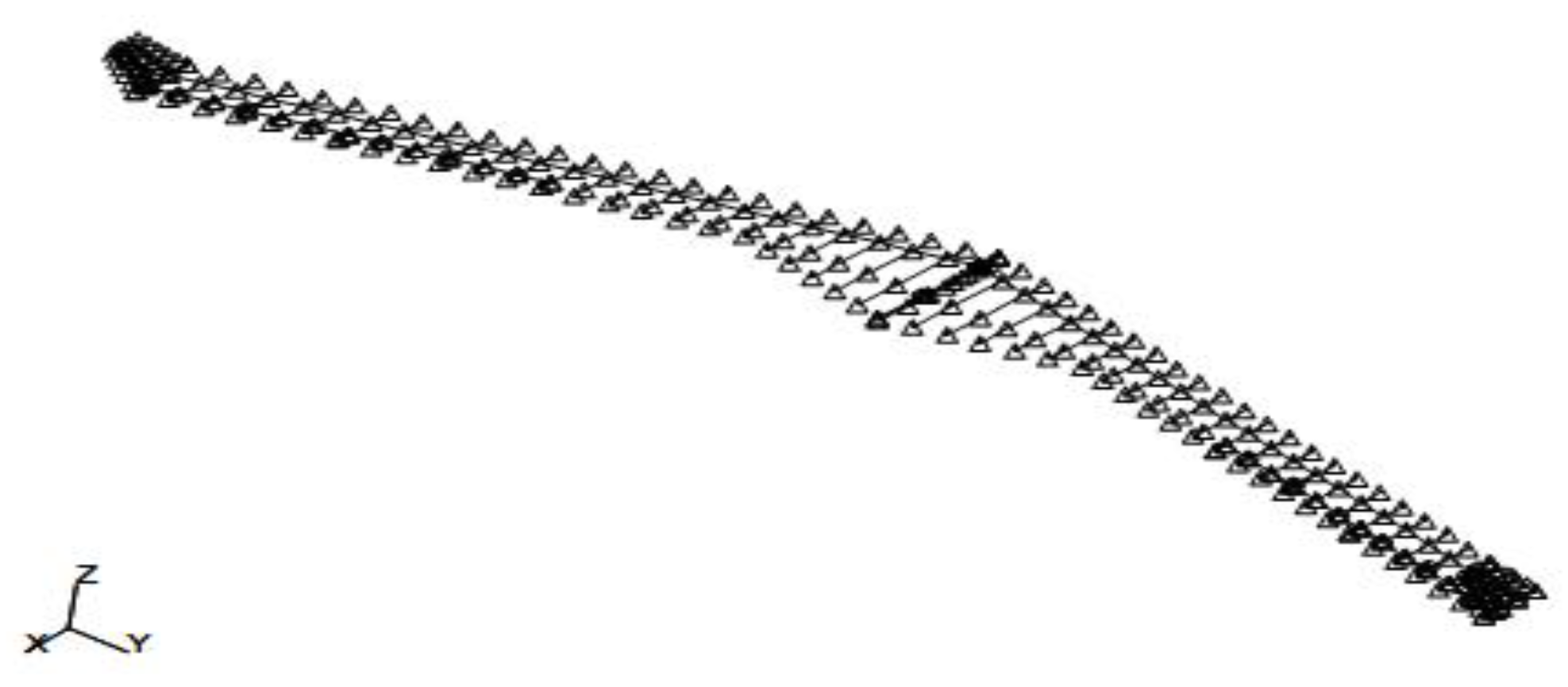
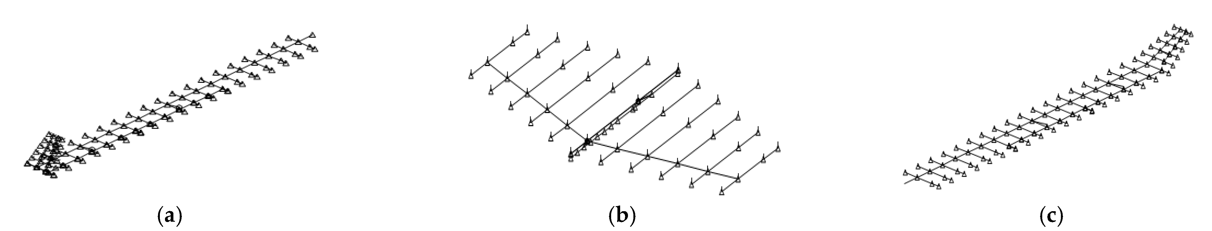
A large flexible aircraft model is presented here to demonstrate the accuracy and efficiency of the proposed method for nonlinear dynamic transient analysis. Static analysis with lateral loads on wing-tip and dynamic transient analysis with harmonic lateral loads on wing-tip are implemented. The response analysis results are compared to nonlinear FEM.

3.1. FEM Model

A large flexible aircraft model with flying wing configuration is presented in Figure 2. Main design parameters are given in Table 1. This aircraft model is composed of a central fuselage fusion with two side wings. The vertical tails are set at each wing tip. The FEM model of the aircraft model is constructed with beam elements and concentrated mass elements. Aluminum is selected as the material of the beam elements and the properties of the material are: E = 73 Gpa, ρ = 2700 kg/m3 and μ = 0.3.
Low order linear mode analysis results of the aircraft model are presented in Figure 3 and Table 2. The first order of elastic mode is 1st symmetric vertical bending mode and the frequency is 3.67 Hz which indicated that the flexibility of the model is high.
With the substructure method proposed, the aircraft model can be divided into the fuselage substructure component, left wing substructure component and right wing substructure component. Three FEM models of the substructures are presented in Figure 4. Low order linear modes analysis results of substructures are given in Figure 5 and Figure 6 and Table 3 and Table 4. The boundary condition of the fuselage substructure model is free condition and the boundary condition of the wing substructure models is root fixed condition. It is consistent with the synthesis method described before. Due to the symmetricity of the aircraft structure, only the right wing substructure analysis results are shown.
The first order mode of the wing component is 1st vertical bending mode and the frequency is 3.58 Hz. Other low order modes also have lower frequencies. In contrast, the first order mode of fuselage is a symmetric mode and the frequency is 49.39 Hz. Wing substructure components are much more flexible than the fuselage substructure component. With the geometric nonlinear problem of the aircraft model, wing components have large deformation under the loads and the fuselage component can be analyzed as a linear component.

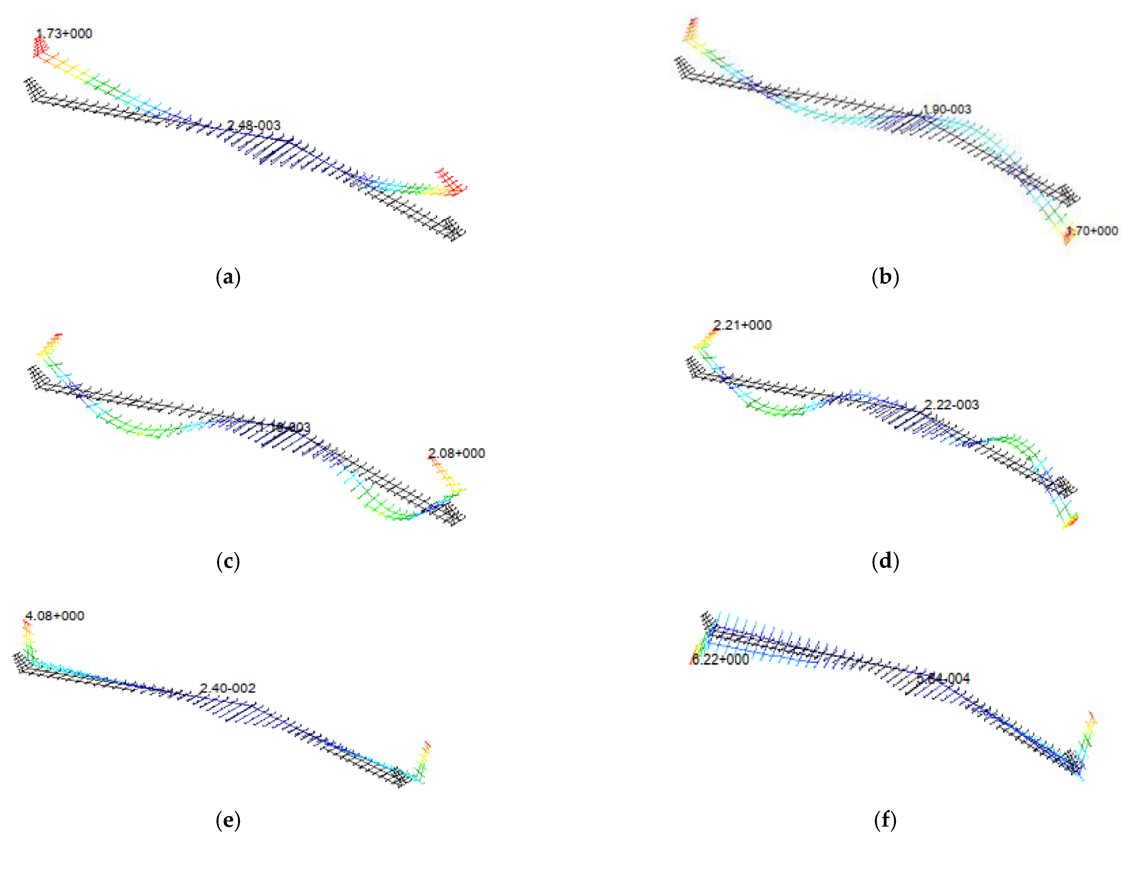
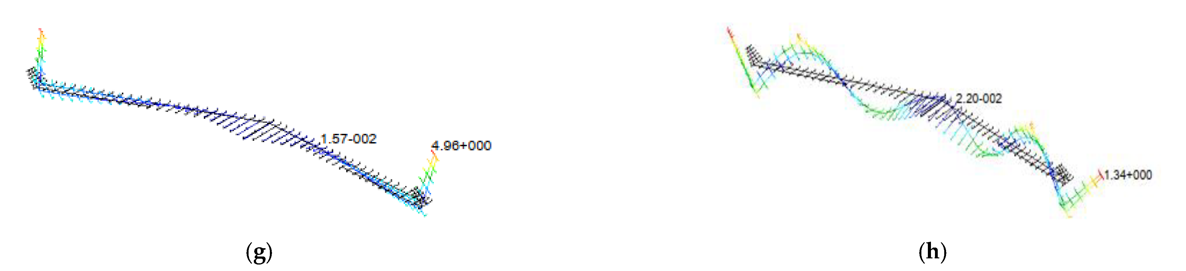
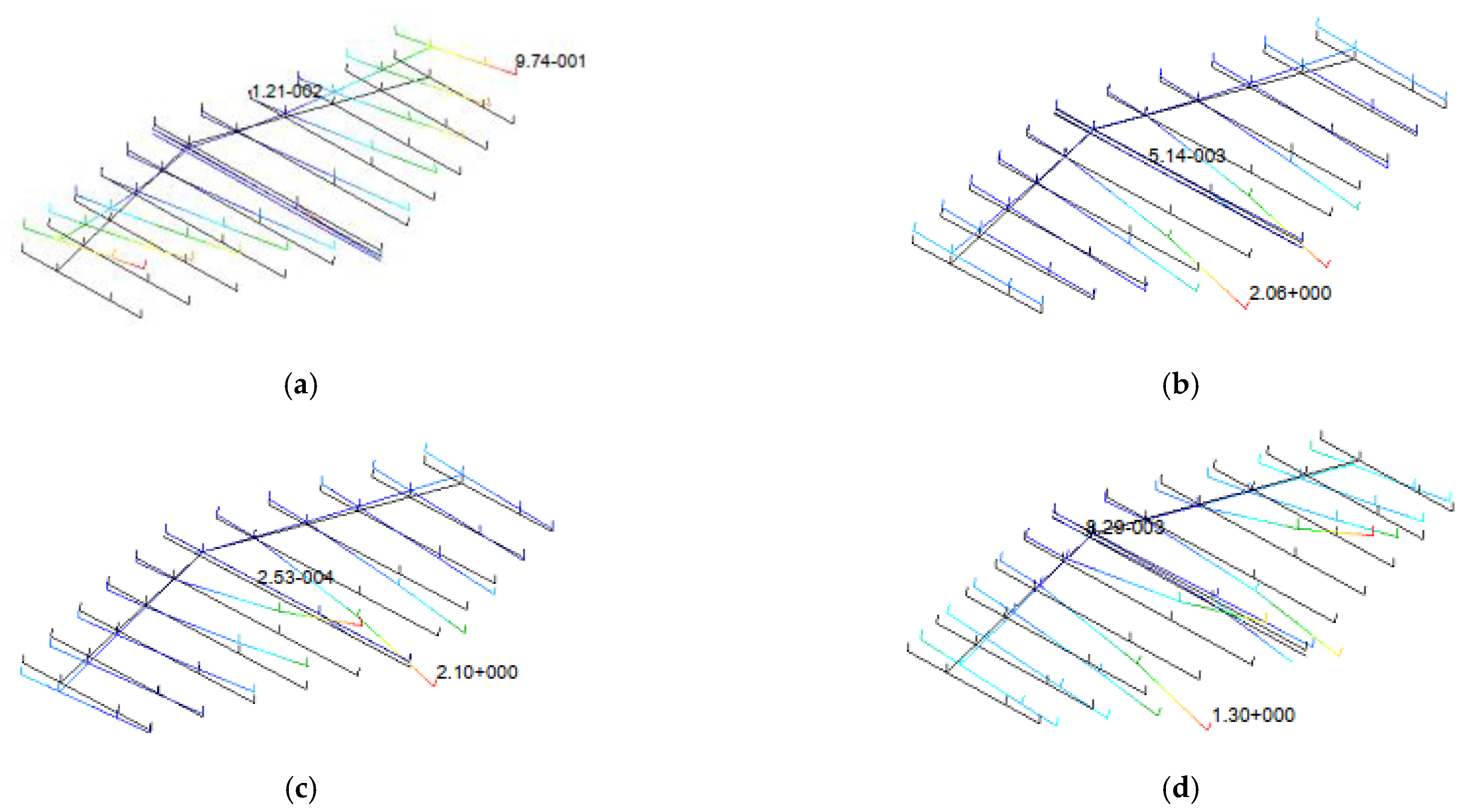
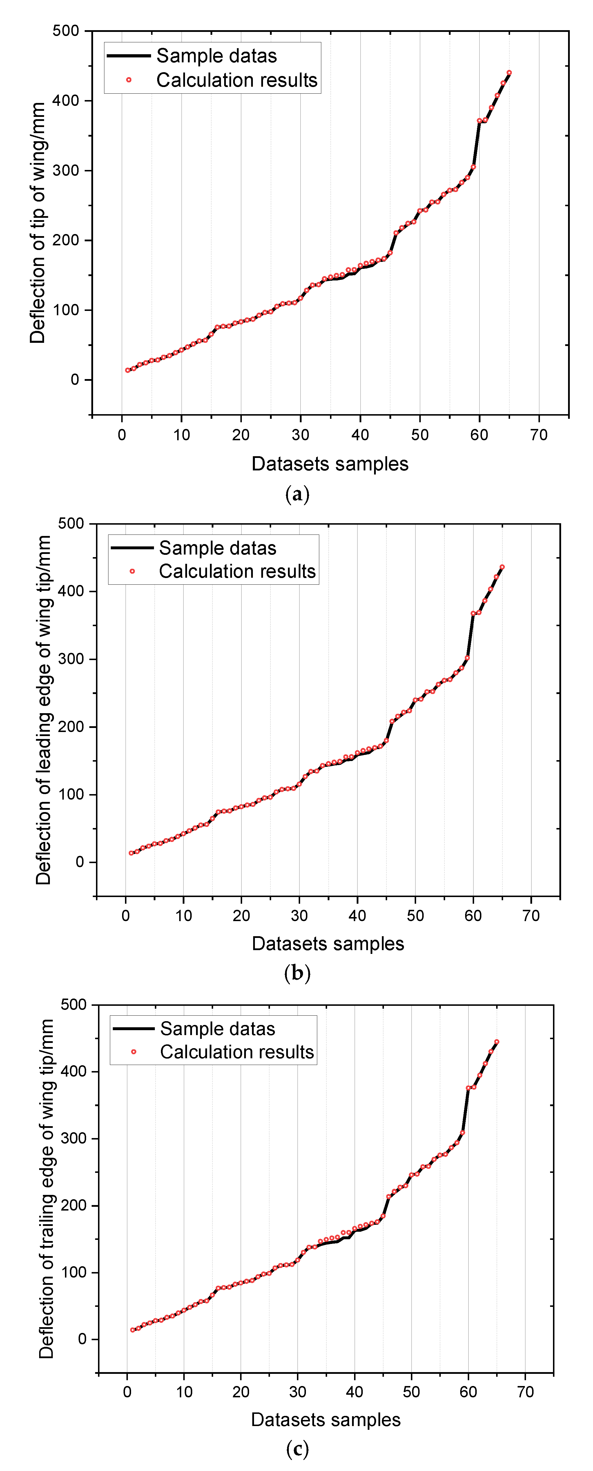
3.2. ROM Model of Wing Components

The ICE technique is used for ROM conduction of the wing component including geometric nonlinearities. The accuracy of the nonlinear component model should be validated before complex structure modeling. The sample datasets used in these numerical examples are generated in MSC.Nastran. The first vertical bending mode and the first torsion mode are selected for generating test load cases with Equation (10). Applied load on wing model structure, corresponding deformation in physical space can be calculated directly. Choosing a series of appropriate scalar weighting factors to satisfy demand of large deformation situations, the test datasets used include 216 samples and the distribution of vertical deflection of the wing tip by sample numbers is shown in Figure 7.
The maximum wingtip deflection in the samples is about 20% of the span length of the wing model. It satisfies the requirement of nonlinear analysis of aircraft structures. The ROM model is validated by predicting the static deformation of the wing model. In this part, 70% (151 samples) of the 216 samples are used for training the ROM model and the remaining 30% (65 samples) are used for validation of the model performance. The least-square technique is used as regression method for finding nonlinear stiffness coefficients. Figure 8 presents the validation results with remaining samples. Deflection in the z direction of the point of the wing tip on the beam, leading edge point of the wing tip and trailing edge point of the wing tip are used for validations. The numbers of validation data samples have been rearranged from small actual values to big values. The prediction results show that the predicted values reach good agreement with actual values. The established ROM model has good performance in large deformation response simulation of wing components.

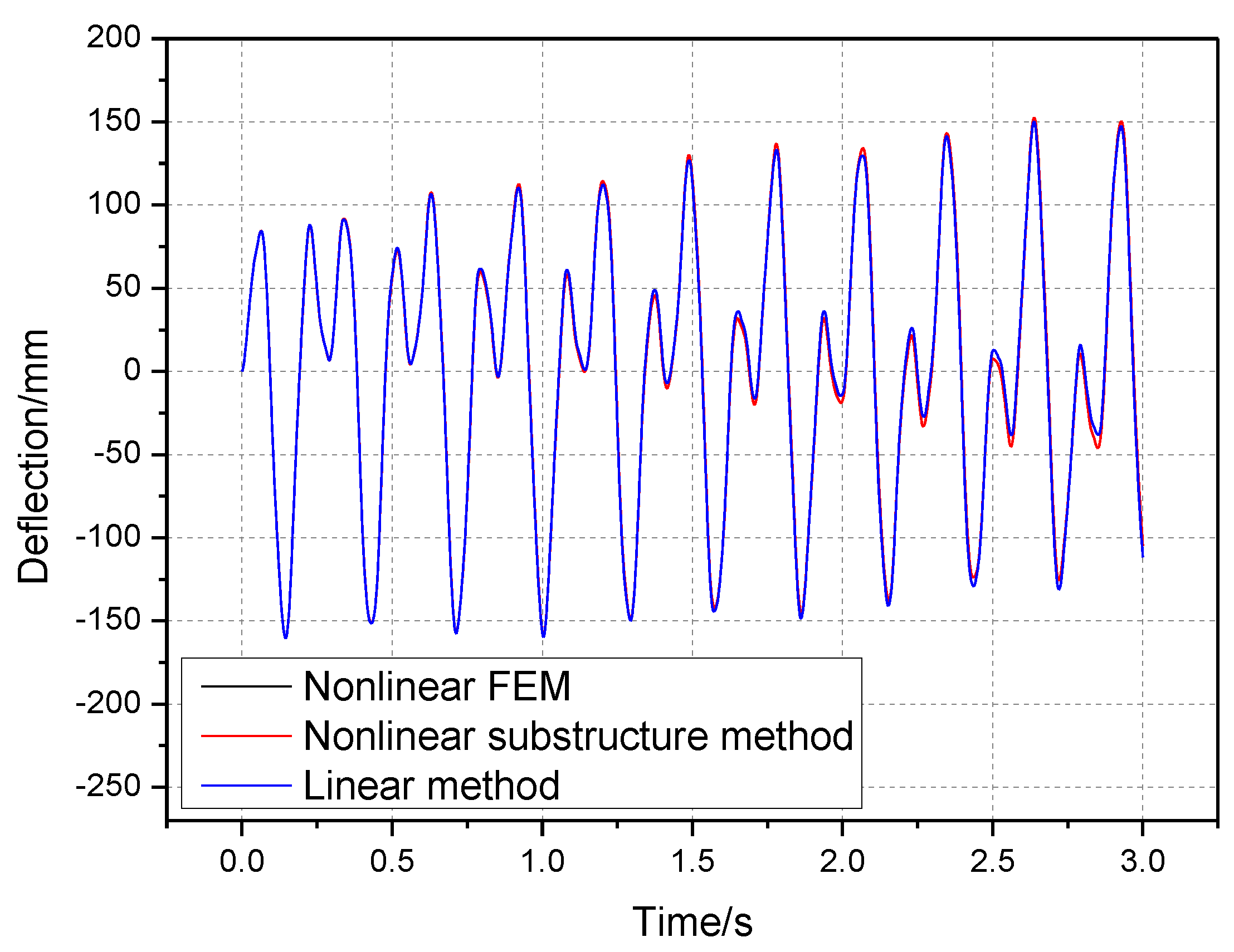
3.3. Response Analysis Results of Aircraft

With the ROM of nonlinear wing components established, the aircraft structure model can be assembled. Nonlinear static and dynamic responses are simulated for validations. In nonlinear static response analysis, lateral loads along the z direction are applied on the tip of the left and right wings. The aircraft model is fixed at the center of gravity. The response analysis results of wing tip deflection are given in Figure 9, using the nonlinear substructure method proposed, nonlinear FEM (full order method, Nastran SOL106) and linear analysis method (full order, Nastran SOL101), up to the load level. It can be seen that the analysis results of the nonlinear substructure method can reach good agreement with the nonlinear FEM. The nonlinear substructure method has obvious advantages in computational cost compared to the full order analysis method. In comparison, the deflection results of the linear analysis are obviously higher than the nonlinear analysis method and the difference gradually increases with increasing load. The linear analysis method is not suitable for modeling the large flexible structures.
In nonlinear transient dynamic response analysis, a harmonic lateral load is applied on the tip of the left and right wings. The boundary condition is the same as static response analysis. The harmonic load F is given as:
F = F 0 sin ( 2 π f t )
where F 0 is the load amplitude and f is the load frequency. The time step of simulation is set as 0.001 s and the total time is 3 s. Nonlinear FEM (full order method, Nastran SOL400) and linear analysis method (full order, Nastran SOL109) are also implemented with the same time step parameters for contrast.
Figure 10 and Figure 11 present dynamic transient analysis results of wing tip with load amplitude 7 N and 20 N. The load frequencies are both 2 Hz. With lower load amplitude, the linear and nonlinear analysis results show no obvious difference. The analysis results using the nonlinear substructure method proposed match well with results from nonlinear FEM.
When the load amplitude increases to 20 N, the geometric nonlinearities lead to an important impact in response analysis. The linear analysis and nonlinear analysis results are obviously different. The analysis results of nonlinear substructure method can still reach a good agreement with nonlinear FEM. In the case of large deformation, the method proposed in this paper shows high accuracy for dynamic response simulation.
Figure 12 and Figure 13 give the dynamic transient response analysis results with a large deformation when changing the load frequencies to 1 Hz and 3 Hz. The load amplitude remains 20 N. Load frequencies are lower than the first order elastic mode frequency and the response deformations increase with increasing load frequency. Figure 14 gives the dynamic transient response analysis results with the load frequency changing to 7 Hz. Load frequency is much higher than the first order elastic mode frequency and the response deformation is small. The analysis results from the nonlinear substructure method still maintain good agreement with nonlinear FEM. It is worth noting that the difference between two nonlinear analysis methods does not change significantly as the response deformation increases. With load frequencies of 1 Hz and 3 Hz, the linear analysis method also leads to obviously different response results when considering geometric nonlinearities as before.
High computing efficiency is an important value for low order models. The computational costs of different methods are presented in Table 5. The nonlinear substructure method spends much less time compared to nonlinear FEM with the same computing hardware (3.40 Ghz, Intel core i7-3770, 8.00 GB RAM). It will be a huge advantage of the application of this method in optimization or aeroelasticity, etc. which needs massive iterative processing.

4. Conclusions

In this paper, a novel nonlinear hybrid interface substructure method with ROM has been developed for dynamic transient response analysis for aircraft structure models with large flexibility. Nonlinear ROM based on ICE techniques is an efficient method for large flexible structure modeling. However, for complex aircraft models, only wing components have large deformation. The analysis can be more efficient and practical if the substructure method can be applied. The method proposed divides the structure into nonlinear substructure components and linear substructure components. The nonlinear substructure components are modeled with ICE techniques and the nonlinear stiffness coefficients are approximated with polynomials. Regression analysis is used for finding the nonlinear stiffness coefficients. The linear components are modeled naturally by linear modes. Each component is assembled by CMS techniques and the boundary conditions of force equilibrium and displacement compatibility are satisfied.
Numerical examples with large flexible aircraft models are presented to validate the accuracy and efficiency compared to nonlinear FEM. Under static loads and dynamic harmonic loads, the analysis results reveal high consistency with nonlinear FEM in both small and large deformation conditions. Meanwhile, the computational time is much lower than nonlinear FEM. The nonlinear substructure method proposed in this paper has high accuracy and efficiency at the same time. It can be used well for large flexible structure response analysis.

Author Contributions

Conceptualization, C.A. and C.X.; methodology, C.A. and Y.M.; software, C.A. and Y.M.; validation, C.X., Y.M. and C.A.; writing—original draft preparation, C.A.; writing—review and editing, C.A. and C.X.; visualization, C.A. and Y.M.; project administration, C.Y. All authors have read and agreed to the published version of the manuscript.

Funding

This research received no external funding.

Institutional Review Board Statement

Not applicable.

Informed Consent Statement

Not applicable.

Data Availability Statement

The data presented in this study are available on request from the corresponding author.

Conflicts of Interest

The authors declare no conflict of interest.

References

  1. Patil, M.J.; Hodges, D.H. On the importance of aerodynamics and structural geometrical nonlinearities in aeroelastic behavior of high-aspect-ratio wings. In Proceedings of the 41st AIAA/ASME/ASCE/AHS/ASC Structures, Structural Dynamics, and Materials Conference and Exhibit (AIAA), Reston, VI, USA, 3–8 April 2000. [Google Scholar]
  2. Eaton, A.J.; Howcroft, C.; Coetzee, E.B.; Neild, S.A.; Lowenberg, M.H.; Cooper, J.E. Numerical Continuation of Limit Cycle Oscillations and Bifurcations in High-Aspect-Ratio Wings. Aerospace 2018, 5, 78. [Google Scholar] [CrossRef] [Green Version]
  3. Tang, D.M.; Dowell, E.H. Experimental and theoretical study on aeroelastic response of high-aspect-ratio wings. AIAA J. 2001, 39, 1430–1441. [Google Scholar] [CrossRef]
  4. Ovesy, H.R.; Nikou, A.; Shahverdi, H. Flutter analysis of high-aspect-ratio wings based on a third-order nonlinear beam model. Proc. Inst. Mech. Eng. Part G J. Aerosp. Eng. 2012, 227, 1090–1100. [Google Scholar] [CrossRef]
  5. Nicolaidou, E.; Hill, T.L.; Neild, S.A. Indirect reduced-order modeling: Using nonlinear manifolds to conserve kinetic energy. Proc. R. Soc. A 2021, 476, 20200589. [Google Scholar] [CrossRef] [PubMed]
  6. Muravyov, A.A.; Rizzi, S.A. Determination of nonlinear stiffness with application to random vibration of geometrically non-linear structures. Comput. Struct. 2003, 81, 1513–1523. [Google Scholar] [CrossRef]
  7. Rizzi, S.A.; Przekop, A. System identification-guided basis selection for reduced-order nonlinear response analysis. J. Sound Vib. 2008, 315, 467–485. [Google Scholar] [CrossRef]
  8. Wang, X.; Mignolet, M.; Eason, T.; Spottswood, S. Nonlinear reduced order modeling of curved beams: A comparison of methods. In Proceedings of the 50th AIAA/ASME/ASCE/AHS/ASC Structures, Structural Dynamics, and Materials Conference, Palm Springs, CA, USA, 4–7 May 2009. [Google Scholar]
  9. Jain, S.; Tiso, P.; Rutzmoser, J.B.; Rixen, D.J. A quadratic manifold for model order reduction of nonlinear structural dynamics. Comput. Struct. 2017, 188, 80–94. [Google Scholar] [CrossRef] [Green Version]
  10. Hollkamp, J.J.; Gordon, R.W. Reduced-order models for nonlinear response prediction: Implicit condensation and expansion. J. Sound Vib. 2008, 318, 1139–1153. [Google Scholar] [CrossRef]
  11. Kuether, R.J.; Deaner, B.J.; Hollkamp, J.J.; Allen, M.S. Evaluation of geometrically nonlinear reduced-order models with nonlinear normal modes. AIAA J. 2015, 53, 3273–3285. [Google Scholar] [CrossRef]
  12. McEwan, M.I.; Wright, J.R.; Cooper, J.E.; Leung, A.Y.T. A combined modal/finite element analysis technique for the dynamic response of a nonlinear beam to harmonic excitation. J. Sound Vib. 2001, 243, 601–624. [Google Scholar] [CrossRef]
  13. McEwan, M.I.; Wright, J.R.; Cooper, J.E.; Leung, A.Y.T. A finite element/modal technique for nonlinear plate and stiffened panel response prediction. In Proceedings of the 42nd AIAA/ASME/ASCE/AHS/ASC Structures, Structural Dynamics, and Materials Conference and Exhibit, Reston, VA, USA, 11–14 June 2001. [Google Scholar]
  14. Kim, K.; Khanna, V.; Wang, X.Q.; Mignolet, M.P. Nonlinear reduced order modeling of flat cantilevered structure. In Proceedings of the 50th AIAA/ASME/ASCE/AHS/ASC Structures, Structural Dynamics, and Materials Conference, Structures, Structural Dynamics, and Materials and Collocated Conferences, Reston, VA, USA, 4–7 May 2009. [Google Scholar]
  15. Feeny, B.F.; Kappagantu, R. On the physical interpretation of proper orthogonal modes in vibrations. J. Sound Vib. 1998, 211, 607–616. [Google Scholar] [CrossRef]
  16. Harmin, M.Y.; Cooper, J.E. Aeroelasic behavior of a wing including geometric nonlinearities. Aeronaut. J. 2011, 115, 767–777. [Google Scholar] [CrossRef] [Green Version]
  17. Cestino, E.; Frulla, G.; Marzocca, P. A reduced order model for the aeroelastic analysis of flexible wings. SAE Int. J. Aerosp. 2013, 6, 447–458. [Google Scholar] [CrossRef]
  18. An, C.; Yang, C.; Xie, C.C.; Yang, L. Flutter and gust response analysis of a wing model including geometric nonlinearities based on a modified structural ROM. Chin. J. Aeronaut. 2020, 33, 48–63. [Google Scholar] [CrossRef]
  19. Xie, C.C.; An, C.; Liu, Y.; Yang, C. Static aeroelastic analysis including geometric nonlinearities based on reduced order model. Chin. J. Aeronaut. 2017, 30, 638–650. [Google Scholar] [CrossRef]
  20. Mignolet, M.P.; Przekop, A.; Rizzi, S.A.; Spottswood, S.M. A review of indirect/nonintrusive reduced order modeling of nonlinear geometric structures. J. Sound Vib. 2013, 332, 62437–62460. [Google Scholar] [CrossRef]
  21. De Klerk, D.; Rixen, D.J.; Voormeeren, S.N. General framework for dynamic substructuring: History, review and classification of techniques. AIAA J. 2008, 46, 1169–1181. [Google Scholar] [CrossRef]
  22. Hurty, W.C. Dynamic analysis of structural systems using component modes. AIAA J. 1965, 3, 678–685. [Google Scholar] [CrossRef]
  23. Craig, R.R.; Bampton, M. Coupling of structures for dynamic analyses. AIAA J. 1968, 6, 1313–1319. [Google Scholar] [CrossRef] [Green Version]
  24. Rubin, S. Improved Component-Mode Representation for Structural Dynamic Analysis. AIAA J. 1975, 13, 995–1006. [Google Scholar] [CrossRef]
  25. Craig, R.R.; Chang, C.J. Free-interface methods of substructure coupling for dynamic analysis. AIAA J. 1976, 14, 1633–1635. [Google Scholar] [CrossRef]
  26. Craig, R.R.; Chang, C.J. On the use of attachment modes in substructure coupling for dynamic analysis. In Proceedings of the 18th AIAA/ASME/ASCE/AHS/ASC Structures, Structural Dynamics, and Materials Conference, Structures, Structural Dynamics, and Materials and Collocated Conferences, Reston, VA, USA, 21–23 March 1977. [Google Scholar]
  27. Kim, D.K.; Bae, J.S.; Lee, I.; Han, J.H. Dynamic characteristics and model establishment of deployable missile control fin with nonlinear hinge. J. Spacecr. Rocket. 2005, 1, 66–77. [Google Scholar] [CrossRef]
  28. Clough, R.W.; Wilson, E.L. Dynamic analysis of large structural systems with local nonlinearity. Comput. Method Appl. Mech. Eng. 1979, 17, 107–129. [Google Scholar] [CrossRef]
  29. Fey, R.H.B.; Van Campen, D.H.; Kraker, D. Long term structural dynamics of mechanical systems with local nonlinearities. J. Vib. Acoust. 1996, 118, 147–153. [Google Scholar] [CrossRef] [Green Version]
  30. Yuan, J.; Salles, L. An adaptive component mode synthesis method for dynamic analysis of jointed structure with contact friction interfaces. Comput. Struct. 2020, 229, 106177. [Google Scholar] [CrossRef]
  31. Apiwattanalunggarn, P.; Shaw, S.W.; Pierre, C. Component mode synthesis using nonlinear normal modes. Nonlinear Dyn. 2005, 41, 17–46. [Google Scholar] [CrossRef]
  32. Bernhammer, L.O.; Breuker, R.D.; Karpel, M. Geometrically Nonlinear Structural Modal Analysis using Fictitious Masses. AIAA J. 2017, 55, 3584–3593. [Google Scholar] [CrossRef] [Green Version]
  33. Kantor, E.; Raveh, D.E.; Cavallaro, R. Nonlinear Structural, Nonlinear Aerodynamic Model for Static Aeroelastic Problem. AIAA J. 2019, 1, 1–13. [Google Scholar] [CrossRef]
  34. Joannin, C.; Chouvin, B.; Thouverez, F.; Ousty, J.P.; Mbaye, M. A nonlinear component mode synthesis method for the compu-tation of steady-state vibrations in non-conservative systems. Mech. Syst. Signal Process. 2017, 83, 75–92. [Google Scholar] [CrossRef] [Green Version]
  35. Laxalde, D.; Thouverez, F. Complex non-linear modal analysis for mechanical systems: Application to turbomachinery bladings with friction interfaces. J. Sound Vib. 2009, 322, 1009–1025. [Google Scholar] [CrossRef] [Green Version]
  36. Kuether, R.J.; Allen, M.S. Nonlinear Modal substructuring of systems with geometric nonlineariteis. In Proceedings of the 54th AIAA/ASME/ASCE/AHS/ASC Structures, Structural Dynamis and Materials Conference, Reston, VA, USA, 8–11 April 2013. [Google Scholar]
  37. Kuether, R.J.; Allen, M.S. Hollkamp, J.J. Modal substructuring of geometrically nonlinear finite-element models. AIAA J. 2016, 54, 691–702. [Google Scholar] [CrossRef] [Green Version]
  38. Kuether, R.J.; Allen, M.S.; Hollkamp, J.J. Modal substructuring of geometrically nonlinear finite element models with interface reduction. AIAA J. 2017, 55, 1695–1706. [Google Scholar] [CrossRef]
  39. Wu, L.; Tiso, P.; van Keulen, F. Interface reduction with multilevel Craig-Bampton substructuring for component mode synthesis. AIAA J. 2018, 56, 2030–2044. [Google Scholar] [CrossRef]
  40. Yang, C.; Liang, K.; Rong, Y.F.; Sun, B. A hybrid reduced-order modeling technique for nonlinear structural dynamic simulation. Aerosp. Sci. Technol. 2019, 84, 724–733. [Google Scholar] [CrossRef]
Figure 1. Connected relationship.
Aerospace 08 00344 g001
Figure 2. Aircraft FEM model.
Aerospace 08 00344 g002
Figure 3. Modal shape of first eight elastic modes. (a) 1st symmetric vertical bending. (b) 2nd asymmetric vertical bending. (c) 2nd symmetric vertical bending. (d) 3rd asymmetric vertical bending. (e) 1st symmetric horizontal bending. (f) 1st asymmetric torsion. (g) 1st symmetric torsion. (h) 3rd symmetric vertical bending.
Aerospace 08 00344 g003aAerospace 08 00344 g003b
Figure 4. Substructure model of left wing component, fuselage component and right wing component. (a) left wing component. (b) fuselage component. (c) right wing component.
Aerospace 08 00344 g004
Figure 5. Wing component modal shape of first four elastic modes. (a) 1st vertical bending. (b) 2nd vertical bending. (c) 1st horizontal bending. (d) 1st torsion.
Aerospace 08 00344 g005
Figure 6. Fuselage component modal shape of first four elastic modes. (a) 1st order mode, symmetric. (b) 2nd order mode, symmetric. (c) 3rd order mode, asymmetric. (d) 4th order mode, asymmetric.
Aerospace 08 00344 g006
Figure 7. Samples of deflection.
Aerospace 08 00344 g007
Figure 8. Prediction of wing tip deflection of wing tip point, leading edge point and trailing edge point. (a) point of the wing tip on the beam. (b) leading edge point of the wing tip. (c) trailing edge point of the wing tip.
Aerospace 08 00344 g008
Figure 9. Static response analysis results.
Aerospace 08 00344 g009
Figure 10. Dynamic transient analysis results with F 0 = 7   N and f = 2   H z .
Aerospace 08 00344 g010
Figure 11. Dynamic transient analysis results with F 0 = 20   N and f = 2   Hz .
Aerospace 08 00344 g011
Figure 12. Dynamic transient analysis results with and F 0 = 20   N and f = 1   Hz .
Aerospace 08 00344 g012
Figure 13. Dynamic transient analysis results with F 0 = 20   N and f = 3   Hz .
Aerospace 08 00344 g013
Figure 14. Dynamic transient analysis results with F 0 = 20   N and f = 7   Hz .
Aerospace 08 00344 g014
Table 1. Design parameters.
ItemValue
Wingspan/mm4800.0
Length of fuselage/mm1033.0
Aspect ratio17.1
Root chord length of wing/mm240.0
Distance between c.g. and node/mm326.0
Width of fuselage/mm1200.0
Weight/kg20.0
Table 2. Elastic modes analysis results.
OrderModeFrequency/Hz
11st symmetric vertical bending3.67
22nd asymmetric vertical bending7.08
32nd symmetric vertical bending20.31
43rd asymmetric vertical bending25.31
51st symmetric horizontal bending31.31
61st asymmetric torsion33.64
71st symmetric torsion34.37
83rd symmetric vertical bending39.61
Table 3. Wing component mode analysis results.
OrderModeFrequency/Hz
11st vertical bending3.58
22nd vertical bending22.31
31st horizontal bending31.97
41st torsion34.95
Table 4. Fuselage component mode analysis results.
OrderModeFrequency/Hz
11st order mode, symmetric49.39
22nd order mode, symmetric92.26
33rd order mode, asymmetric94.04
44th order mode, asymmetric111.05
Table 5. Computational time with different method.
Computational TermNonlinear FEM/minNonlinear Substructure Method/min
F0 = 20 N and f = 2 Hz402.5
F0 = 20 N and f = 1 Hz342.3
F0 = 20 N and f = 3 Hz654.5
F0 = 20 N and f = 7 Hz352.5
Publisher’s Note: MDPI stays neutral with regard to jurisdictional claims in published maps and institutional affiliations.

