1. Introduction
In the previous decades, schemes enabling the staggered (partitioned) coupling between linearized low fidelity aerodynamics and structural mechanics have been the workhorse of the computational aeroelastic community.
Low solution turnaround time compared with solution schemes utilizing higher fidelity aerodynamics, greater robustness compared to monolithic schemes, and the ability to treat each discipline separately using different specialized techniques have highly contributed to this end. Such coupling schemes represent the current state-of-the-art in computational aeroelasticity [
1,
2].
However, progress in lightweight materials leading to wings of constantly increasing flexibility and aspect ratio, aiming at significant fuel savings, the inclusion of a variety of continuous deformation morphing devices, and a tendency for modern airliners to operate near the transonic region have placed renewed emphasis on using higher fidelity aerodynamics in computational aeroelastic solutions.
Differences in the results for divergence and flutter limits, as well as the predicted aerodynamic loads between solutions obtained using high and low fidelity aerodynamics for such cases were pinpointed in [
3,
4].
The ability of linearized aerodynamics to accurately predict the aeroelastic behavior for future wing configurations is therefore in doubt and must be evaluated on a case-by-case basis, as outlined in several studies [
5,
6].
As a direct consequence, finding ways to efficiently integrate high fidelity aerodynamics into aeroelastic packages represents a current serious challenge in the field of computational aeroelasticity [
2,
7].
Using high fidelity aerodynamics bears the promise of sufficiently tackling future aeroelastic problems, even in cases where the validity of low fidelity aerodynamics degrades quickly.
Such cases include aeroelastic analyses in regions with strong non-linear flow effects, the treatment of very high aspect ratio wings exhibiting high deformation magnitudes relative to their span, and cases where panel methods fail to provide aerodynamic results of sufficient accuracy for the intended use.
The inability of linearized low fidelity aerodynamics to capture the aeroelastic behavior in the transonic region (most notably, differences in predicting the transonic dip in dynamic aeroelastic analyses compared to non-linear methods) has been well documented [
8]. Due to their formulation, linearized aerodynamics were never designed to capture aerodynamic non-linearities such as shock waves that form in the transonic regime. Therefore, substantial deviation in the response compared to using high fidelity aerodynamics can occur. Surprisingly, the differences in the results between lower and higher fidelity aerodynamics in static aeroelastic analyses have not been studied as thoroughly [
5].
Other cases where the flow physics cannot be accurately described with low fidelity aerodynamics or semi-empirical formulations include flutter arising from separated flow as is the case of rotor blades [
9] and vortex-boundary-shock interactions and aeroelastic instabilities that are caused by aerodynamic-nonlinearities during maneuvering of fighter aircraft primarily [
10].
The very high aspect ratio wing configuration is one of the candidates for future unconventional aircraft wing geometries. Due to the high non-linear deformation exhibited by such wings, the aerodynamic behavior changes significantly during deformation. Low fidelity aerodynamic models including various degrees of aerodynamic non-linearity have been adapted to the above cases; however, the results have been shown to be less accurate compared to time domain solutions using high fidelity aerodynamics. A trend toward overly conservative predictions due to underestimating the aerodynamic damping and significant differences in the aeroelastic deflections have been highlighted in several studies [
4,
11].
Finally, the detail in the flow field solution that can be achieved with a low fidelity aerodynamic analysis (for example, using panel methods) can be insufficient for the aeroelastic optimization and tailoring of a flexible structure, particularly if local effects are considered. Considering fluid-structure interaction during the design optimization of aeronautical structures has been shown to lead to significant gains in performance.
In [
12], fluid–structure interaction solutions using Reynolds-averaged Navier–Stokes (RANS) aerodynamics were included in the geometry optimization procedure for a supersonic missile. An improvement in the range from 3–5.6% was realized as a result. Further work on this optimization study [
13] led to even higher gains in maximum range by modeling the thermoelastic problem.
Properly treating the thermoelastic problem at the supersonic velocity range typically requires high fidelity solutions in order for the high temperature gradients near shock wave and expansion regions to be captured.
The above emphasize possible gains from the inclusion of high fidelity aerodynamics in the fluid–structure interaction even in flow regimes where the usage of low fidelity formulations is not necessarily considered prohibitive from a purely aerodynamic perspective.
Therefore, the use of high fidelity aerodynamics within aeroelastic optimization frameworks has become a modern and active research topic [
11]. Despite the additional solution detail, such use has remained to date limited [
14].
Utilizing high fidelity aerodynamics in computational aeroelasticity, although attractive, comes intertwined with serious challenges. The most important are the ability to deform an aerodynamic mesh extending to the domain’s boundaries while preserving sufficient quality, the extremely high computational cost per solution, and the unintuitive representation of the results as values of several variables in millions of degrees of freedom.
Reduced order models striving to describe the aeroelastic behavior of the wing by using only a few physically rich in information degrees of freedom bear the promise of addressing those issues to some extent.
Such models can be based on signal theory [
15], mathematical decomposition techniques [
16], and machine learning.
ROMs based on Volterra series theory borrowed from the field of signal theory and using the formulation of Silva and Bartels [
17] will be considered in this work, albeit without casting the aerodynamic impulse responses in the frequency domain. Thus, time domain Volterra ROMs are formulated.
The validity and computational cost-effectiveness of Volterra series reduced order models in treating static aeroelastic cases of increasing complexity will be investigated. Such reduced order formulations have been used in the literature mainly as a cost effective way of including high fidelity aerodynamics in treating dynamic aeroelasticity. Although theoretically static aeroelasticity can be treated with the same tools, a gap in providing such solutions, including a comparison with tried and trusted techniques, as well as identifying the advantages and potential shortcomings of such an approach specifically for the static aeroelastic case exists.
Additionally, an attempt is made to outline a methodology for constructing such reduced order formulations using tools already available in commercial computational analysis packages, without the need for specialized in-house software. This is considered beneficial for the wider application of such techniques.
The main aim is the investigation of the Volterra series reduced order models as an intermediate “medium computational cost” step between “low computational cost” solutions with linearized aerodynamics and “high computational cost” full staggered coupled solutions for the static aeroelastic case.
In the present paper, the computed static aeroelastic response of composite plates exhibiting varying torsion-bending coupling [
18,
19], the AGARD 445.6 wing [
20], and the high Reynolds number aerostructural dynamics (HiReNASD) configuration [
21] are presented, including validation against theoretical, experimental, or computational results, depending on their availability.
Furthermore, the flexibility of the ROM in providing solutions to variations of the dynamic pressure and the modification of basic parameters for the structure such as natural frequencies, amplitudes, and damping ratios are outlined. The reduced order model formulation provides a handy tool to evaluate the deviation in the final solution due to discrepancies in each aforementioned parameter. Potential uses include evaluating the deviation between numerical and experimental results due to such discrepancies or taking mild structural changes into account (for example, eigenfrequency shifting due to structural aging or stiffness variations).
2. Materials and Methods
2.1. Treatment of the Structural Component
Finite element analysis assuming linear behavior was used to treat the structural problem, while thermal effects and geometric and material non-linearities were neglected.
For the general structural analysis problem, the governing equation has the following form:
where:
| , the vector of external loading. |
| , the stiffness, damping, and mass matrices. |
| , the displacement vector. |
| | | |
For the static solution, the mass and damping terms are excluded. Another way of efficiently solving the static problem is by using the critical damping method, in which the output quickly converges to the steady state. This will be exploited to solve the static aeroelasticity problem, by a reduced order model that contains the general form of the structural governing equations.
If the behavior of structural deformation remains linear, the structural governing equations can be cast into the modal space. Using the superposition principle and writing the equations in state-space form, the following description of the structural system is obtained:
where:
| , the state variable containing the generalized displacements and their derivative; |
| , the input variable containing generalized forces; |
| , the zero and diagonal unity matrix; |
| , a diagonal matrix containing the natural frequencies squared; |
| , the modal damping factor. |
| | | |
This form is advantageous because it consists of a very efficient reduced order model for the structure that can be easily coupled to an aerodynamic system to fully describe the aeroelastic system.
For structural systems with strong non-linearities or complex damping where the linear superposition of mode shapes is no longer valid, using a Volterra series expansion is a feasible option. This procedure is covered in detail for the aerodynamic system in
Section 2.4, but is also applicable to the structural side.
2.2. Treatment of the Aerodynamic Component
The Euler equations, discretized using the finite volume method (FVM), were solved for the composite plate and AGARD 445.6 wing in incompressible and compressible form, respectively. For the HiReNASD configuration, both inviscid Euler and viscous Navier–Stokes formulations were evaluated. Higher order upwind schemes were preferred due to their numerical stability. The general form of the compressible Euler equations is presented below:
where:
| , the density; |
| , the velocity vector; |
| P, the total pressure; |
| E, the total energy. |
Convection terms were discretized using second order upwind or QUICK(4th order upwind) schemes. Source terms were discretized using central differences. An implicit first order difference scheme was chosen for the temporal discretization.
An algebraic multigrid was not used from the onset of the impulsive input and until the solution converged to steady state, as it has been shown to lead to extra diffusion when obtaining the necessary impulse responses for the reduced order model, thus adding extra artificial damping in the response [
22].
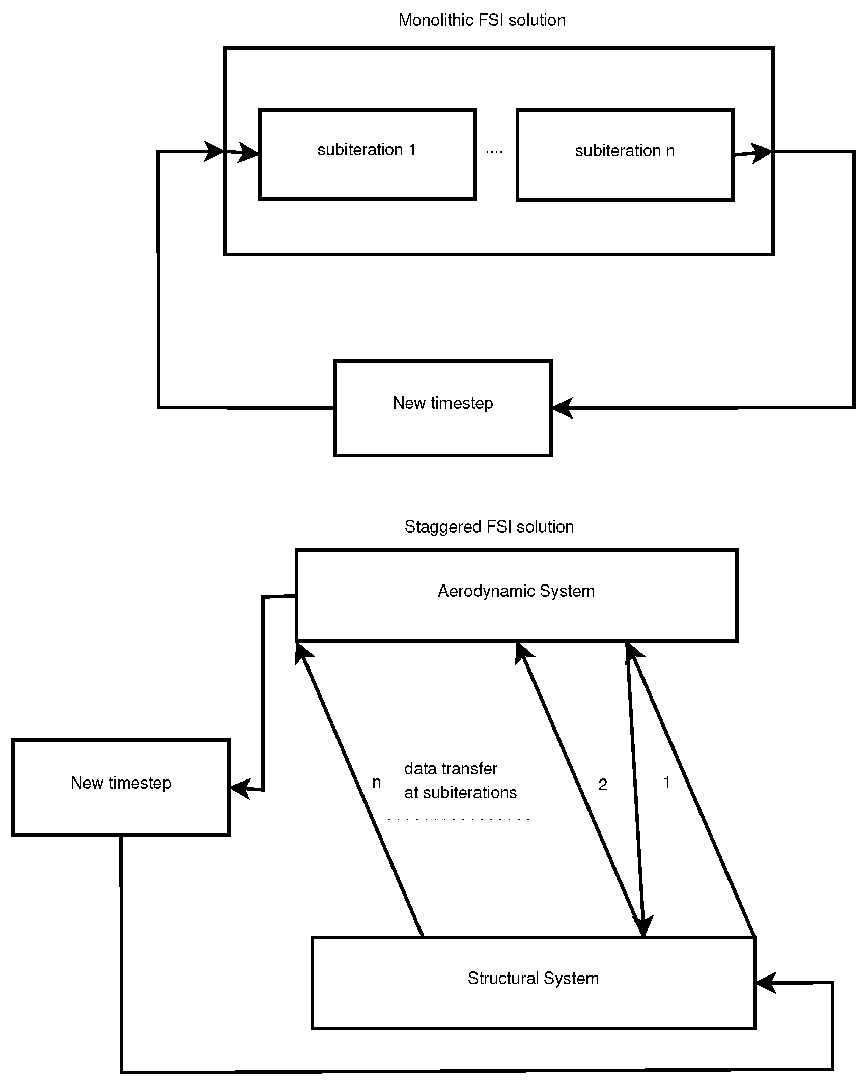
2.3. Coupling Scheme
For coupling the structural and fluid problem, two main approaches exist. These are the staggered or partitioned approach and the monolithic approach (
Figure 1).
In the monolithic approach, a single mesh is used, and both problems are solved simultaneously. In the staggered approach, the two systems are treated and solved successively. After the solution of each discipline, the results are transferred to the other one, and the solution thus advances iteratively in time. The current work employs a staggered approach.
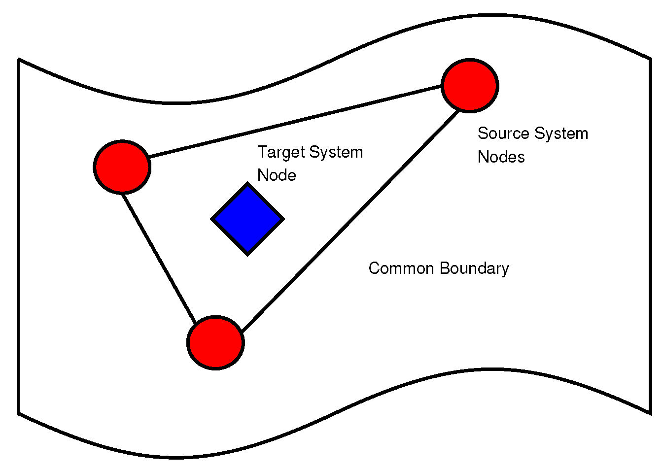
A common boundary in both the structural and fluid part needs to be defined, facilitating the data exchanges, and a robust mapping technique should be used to transfer the results between dissimilar meshes.
By projecting the fluid dynamics and structural mechanics nodes upon the common boundary, a finite element approximation for transferring the loads can be formulated. Each transfer element consists of nodes from the source system and a node from the target system (
Figure 2). The result is a transfer matrix that maps every node of the structural system to the aerodynamic one and vice versa.
Special consideration must be given to ensure the conservation of work when transferring the loads. For transferring structural displacement or point loads, a simple finite element shape function or distance based interpolation is enough to ensure conservative mapping.
However, when transferring surface loads such as pressure, the simple distance based interpolation fails to automatically ensure the conservation of work. That happens because it is not the nodal distance, but rather the overlap between target and source elements that dictates the portion of the load that each source element should contribute to the target element.
Techniques like general grid interpolation (GGI) that use simple distance based interpolation for transferring point loads, but take the overlap into account when transferring surface loads have been used widely in commercial analysis software.
Commonly, the quality of the load transfers is determined by the percentage of nodes and the area of each system successfully mapped onto the other system. Factors near 100% are desirable.
On the common boundary, the compatibility conditions must be enforced at each data transfer:
where:
| | the mapping between structural displacement and displacement |
| | | of the boundary CFD nodes; |
| | the structural surface stress at the common boundary resulting from |
| | | the pressure exerted by the fluid. |
Unlike the structural mesh, deforming the fluid domain without deterioration of mesh quality is a serious challenge.
The spring based deformation algorithm using Laplacian smoothing and remeshing criteria can be used to handle the mesh deformation for the aerodynamic mesh away from structured prism layers that are set to deform as a rigid body with the boundary.
The small amplitude of the impulse functions needed for the reduced order model are also beneficial in preserving mesh quality.
Furthermore, to reduce the numerical error resulting from the staggered nature of the solution, each time step was set to contain a number of at least 7 coupling sub-iterations for the full staggered coupled solutions.
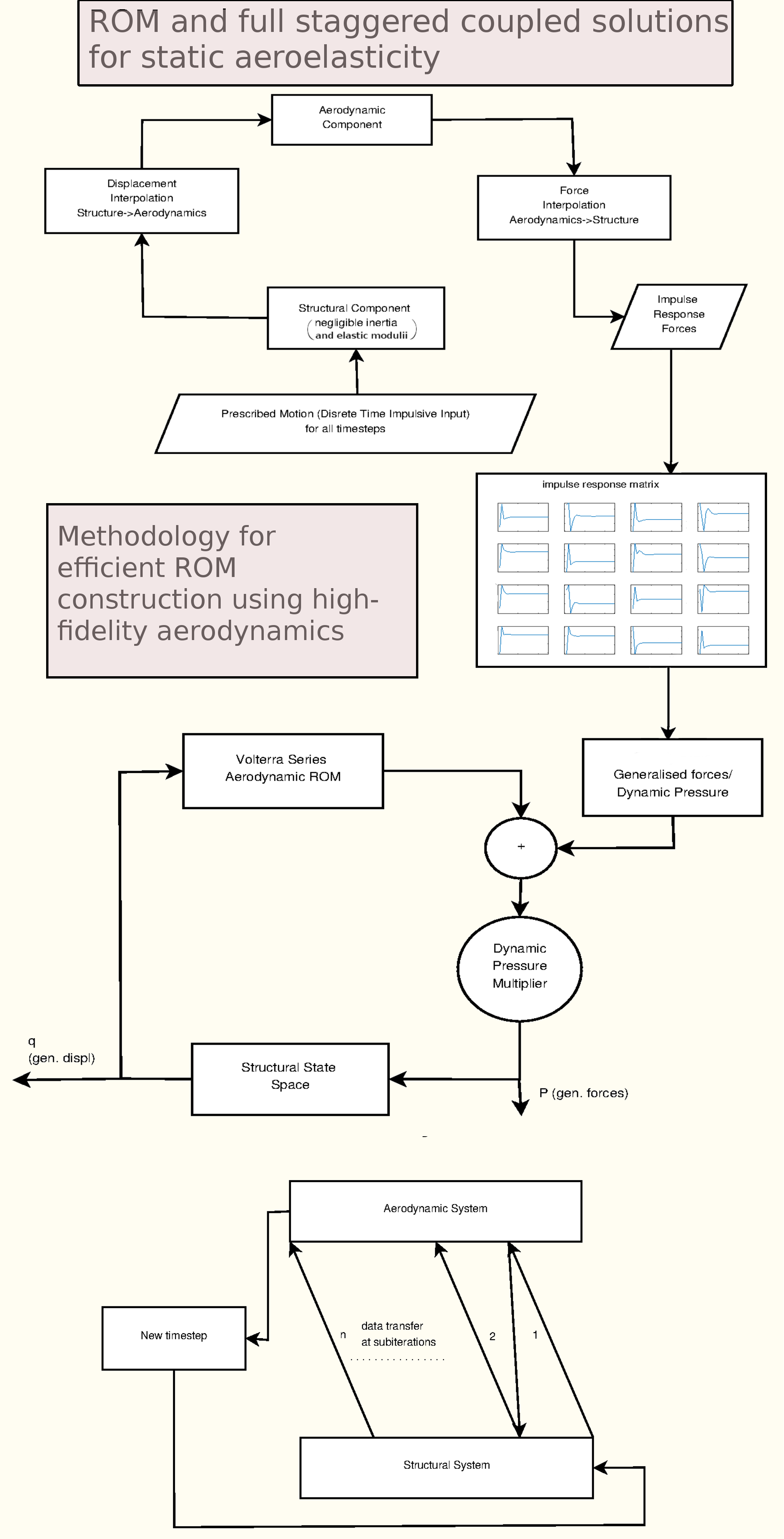
2.4. Development of the Reduced Order Model
A linear reduced order model for the aeroelastic systems considered was built using the Volterra series approximation as formulated in [
17].
By examining Equation (
1), it is evident that the aerodynamic part required to fully describe the closed loop aerostructural system and enable development of the reduced order model must correlate the time history of the state variables (generalized displacements of selected mode shapes) to a resulting time history of the excitation (generalized forces resulting from the time history of the state variable).
The Volterra series theory states that the response of a time-invariant system with memory effects to an arbitrary input can be expanded into a series using kernels containing the linear and non-linear impulse responses of the system. In discrete time, it has the following form:
where:
| , the output and input variables; |
| , the steady state response; |
| h, linear and non-linear convolution kernels. |
Some level of the response of a weakly non-linear system may be captured with the first order kernel that is different from a purely linear kernel. Weakly non-linear systems have been successfully approximated in this manner [
22].
The impulsive input to the unsteady aerodynamic system, corresponding to the excitation of each generalized coordinate, is proven to be well defined in the discrete time domain and modeled as [
17]:
Small amplitudes may be used with this method, and the final impulse response is obtained by scaling [
17]. Engineering judgment should be applied to only scale that part of the force response that is dominated by the impulse and to avoid scaling the part away from the structural input that consists of small amplitude numerical noise around a converged force value. Otherwise, incorrect higher amplitudes in the aeroelastic deflections may be obtained due to the extra spurious energy that is inserted into the ROM. In the present work, the RMS difference in transferred loads was used as a criterion to distinguish these two regions; the scaling terminated at the exact point where the RMS change fell to the level of the time history before the impulsive input.
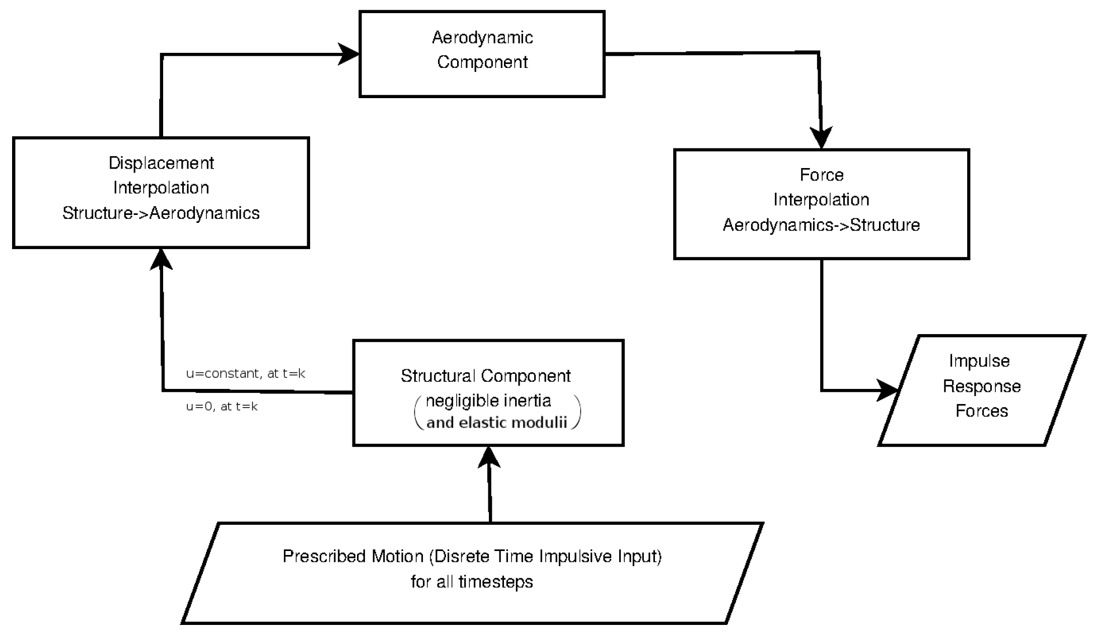
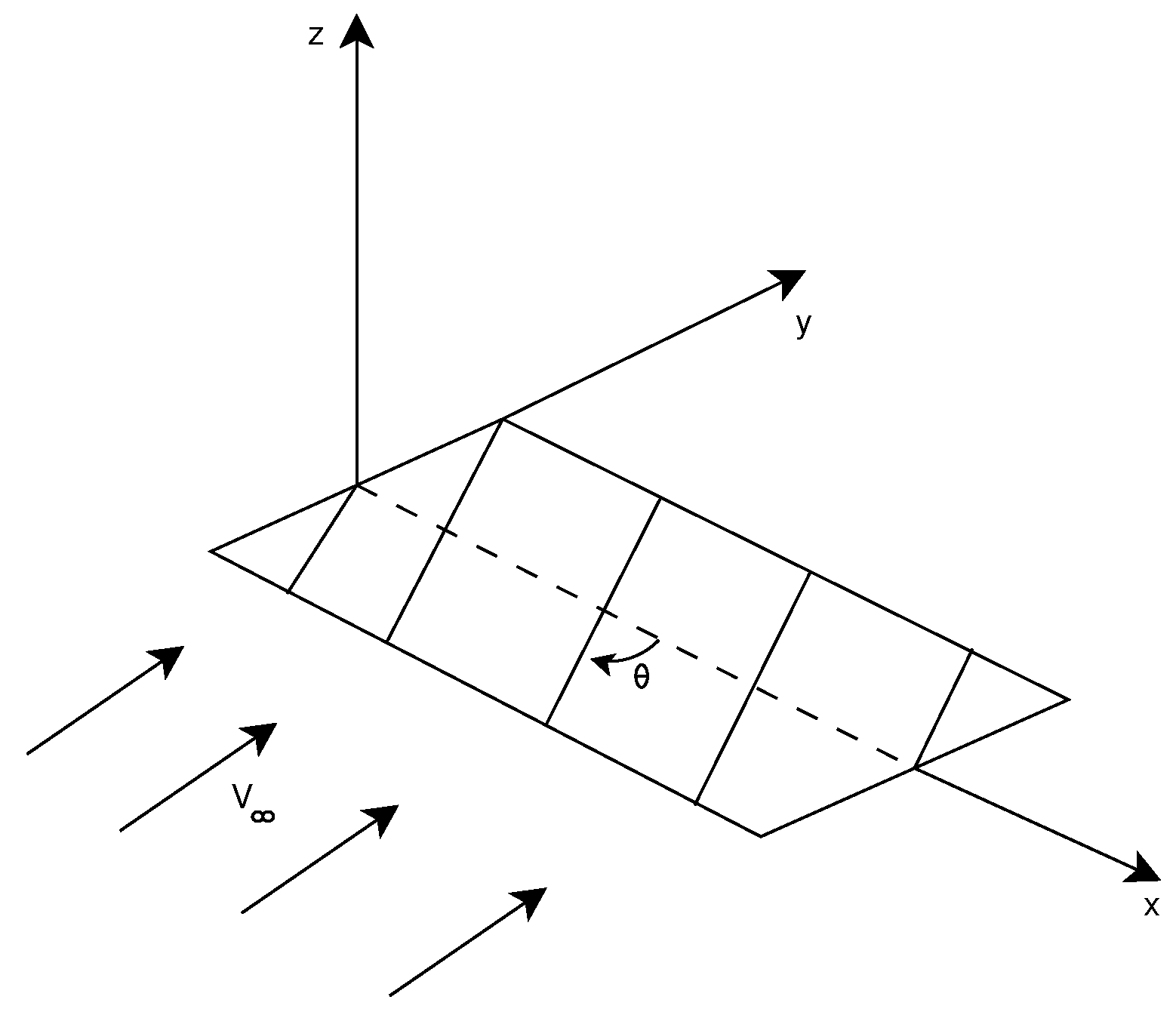
In the scope of this work, the impulsive input to each mode will be represented as prescribed structural deformation in the structural solver. The data transfer algorithm will then pass the necessary deformation to the aerodynamic mesh. This deformation is per Equation (
7) of constant modal amplitude at time step k and fixed at zero for all other time steps. The entire structure is fixed at either a constant modal amplitude or at a zero one at any point in time (
Figure 3).
By using negligible inertial and elastic moduli and no damping on the structural side, the structural loads that would result from the motion of the structure are in turn negligible. From Equation (
1) for negligible inertial and stiffness moduli and no damping:
Thus, only the unsteady aerodynamic loads that are passed from the aerodynamic system are significant at any given time. Either nodal forces or reactions can be captured to obtain the unsteady aerodynamic forces interpolated on the structural system’s mesh.
Due to the motion at each time step being prescribed at all nodes to satisfy Equation (
7), no computational issues arise from the negligible inertial and elastic properties. It should be noted that this “modified” structural system is used only as a means of interpolating the impulsive inputs onto the fluid mesh and capturing the unsteady aerodynamic loads. It is not the structural system that is coupled with the unsteady aerodynamic one to form the final aeroelastic ROM.
This methodology allows using boundary motion interpolation tools between the structural and aerodynamic system, which are already present in most modern computational aeroelasticity frameworks, thus providing robustness, consistency, ease of use, and a straightforward way to integrate such a reduced order modeling technique into the current fluid-structure interaction analysis framework without major disruption.
The impulse responses were calculated around a steady state condition for the FSIproblem at a certain Mach number value. The ROM retains validity around this Mach number.
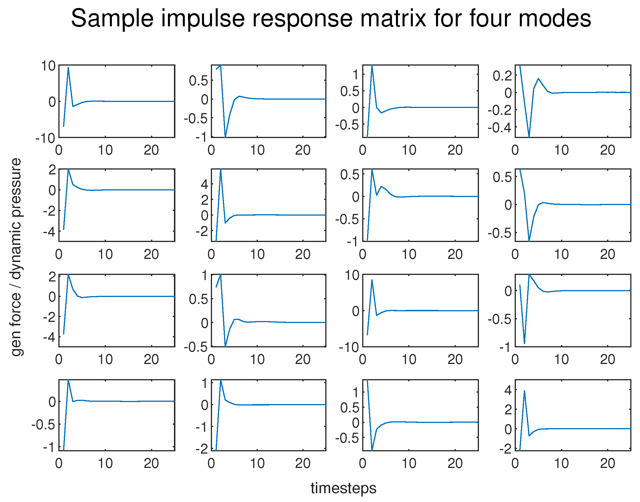
Calculating the necessary impulse responses for all modes from the excitation of each particular mode, the Volterra series reduced order model was built and coupled with the structural side. In the case of a linear model, this reduces to a convolution matrix (
Figure 4):
The diagonal terms represent the generalized force response of each mode due to the excitation of the same mode and as expected provide the dominant values of the matrix. The remaining terms represent the generalized force response of mode i due to an excitation in mode j and therefore are coupling terms.
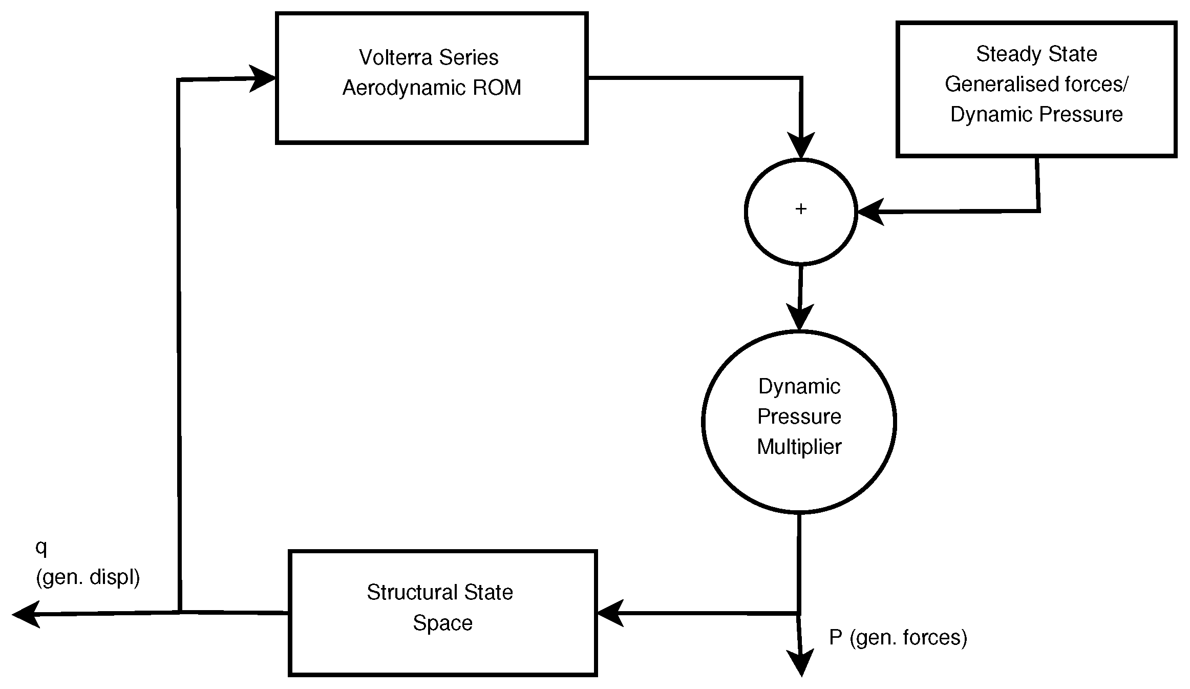
The outline of the Volterra series time domain reduced order model is shown below in
Figure 5.
3. Results
The applicability of the same ROM during variations in dynamic pressure around a specific Mach number provided that the physics of the flow remain similar without the need for calculating new sample data and its validity when modifying damping factors and natural frequencies are discussed. In particular, the validity of the reduced order model to variations of the dynamic pressure is examined during the treatment of Case (c), while the ability to readily and cost-effectively incorporate variations in damping factors and natural frequencies of the structure is highlighted during the treatment of Case (b).
3.1. Composite Plate Wing Analysis
A numerical investigation of the plate wings reported in [
18] and in particular those with orientations of
,
and
was performed. Different ply orientations result in varying bending torsion-coupling and, as a result, a different aeroelastic response. This is important in practical applications [
23], and consequently, the ability to capture such an effect with the aeroelastic methodologies of the present study will be demonstrated.
These plates were tested at low subsonic velocities. As a consequence, incompressible flow was assumed. Furthermore, to augment the numerical stability in the computational fluid dynamics (CFD) runs and enable reaching a robust steady state, the plate was incorporated in a styrofoam fairing with the shape of a NACA0012 airfoil. Due to the stiffness of the basic graphite-epoxy material being an order of magnitude higher, the effect on the results is expected to be minimal.
Even though steps to minimize numerical error were undertaken (such as the grid convergence study provided in
Table A2), a comparison of exact values between experiment and the present case is problematic.
Due to the unavailability of information regarding important experimental parameters (free stream density), some uncertainty regarding how accurately the experimental conditions were replicated in the computational model is inevitable. The approximate calculation of wingtip deflection in the original experiment presents an additional potential cause of differences between the numerical, theoretical, and experimental results.
On the numerical side, factors contributing to those differences (other than the spatial discretization) include the number of mode shapes used in the reduced order model, the time step, and methods used for the temporal discretization of the impulse responses. Therefore, the comparison should be limited to response trends for this specific case.
High fidelity CFD is not a requirement for this simple incompressible flow case. However, these experimental and theoretical results present a good opportunity to validate that the influence of the varying bending-torsion coupling behavior due to the ply orientations is captured in the aeroelastic response using the ROM scheme before investigating more complex cases. The simplicity of the aerodynamic system is deemed beneficial for this reason.
The plate geometry was taken from the original paper [
18] and is presented along with the fiber orientation system used in
Figure 6.
The following
Table 1 and
Table 2 contain an overview of the geometry, material data, and computational analysis envelope.
Reasonable agreement in the first three eigenmodes and frequencies was established between the computational modal analysis of the present study and the actual experiment for the three laminates, as is evident in
Table A1. As expected, the inclusion of the styrofoam fairing did not lead to significant changes to the dynamics of the system.
The lift coefficient for the undeformed plate was compared to the results from theoretical relations for finite wing aerodynamics using the thin airfoil theory assumptions in
Table A3.
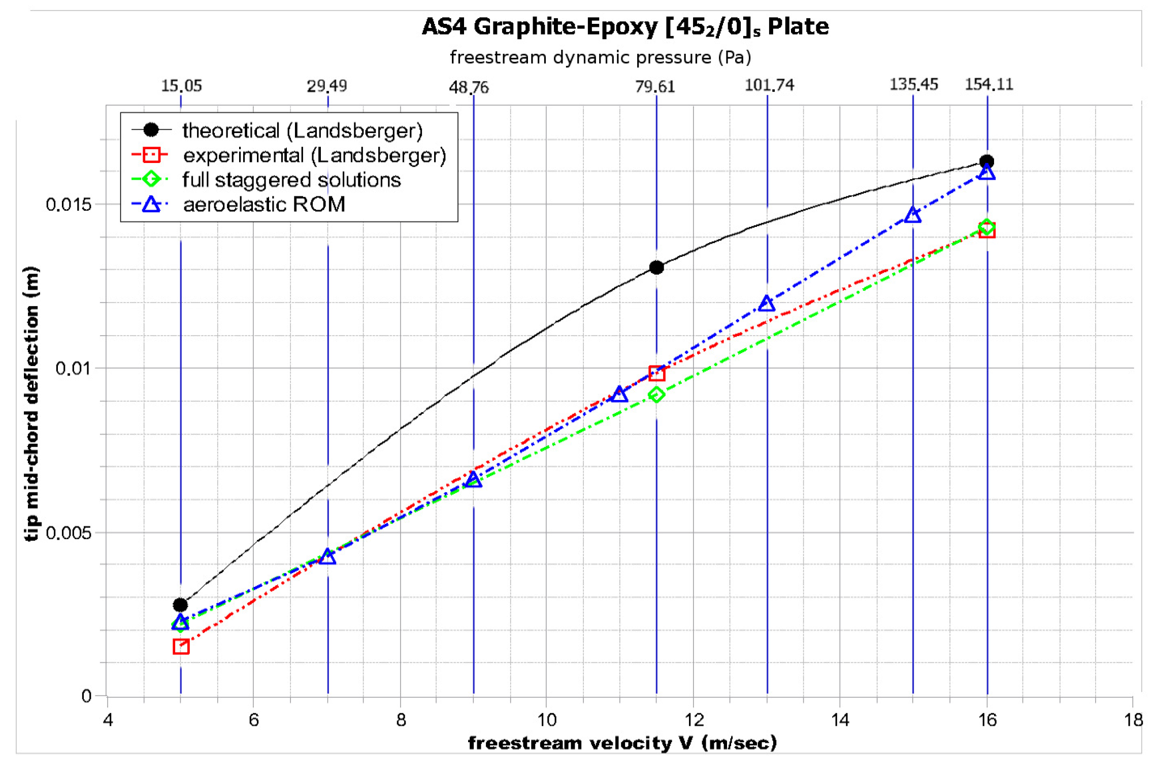
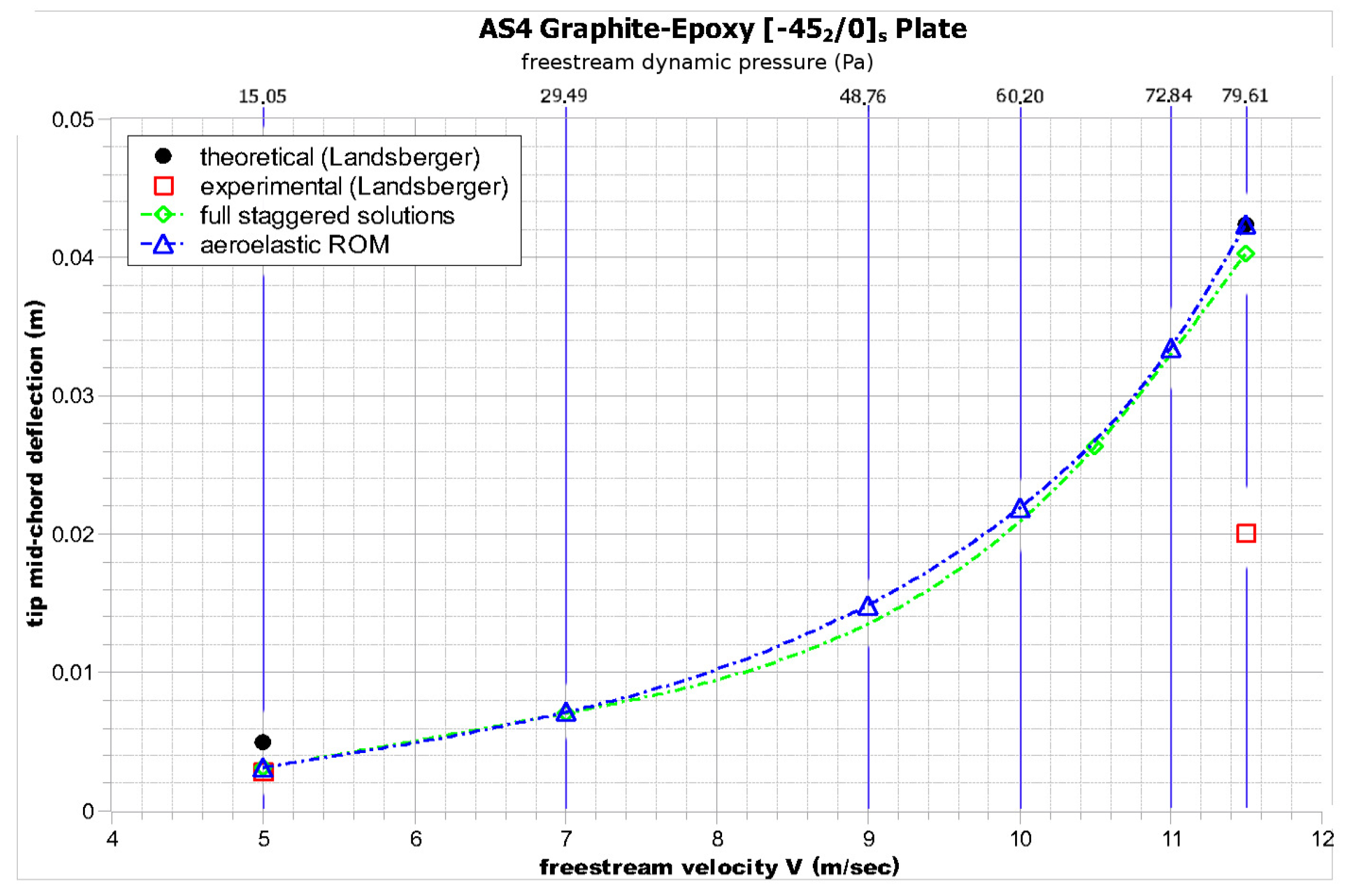
The static aeroelastic deflection in the mid-chord location of the tip for all the laminates is presented in the subsequent figures for the flow conditions that are summarized in
Table 3.
As can be seen in
Figure 7,
Figure 8 and
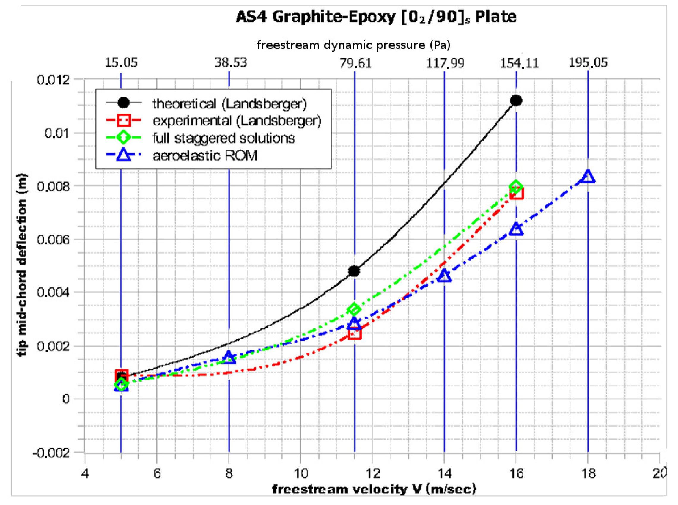
Figure 9, the general trend of the aeroelastic tip deflection with the increase in velocity is captured relatively well by both the reduced order model and the full staggered solution:
The plate wing exhibits the smallest tip deflection as a result of having the highest amount of unidirectional plies oriented along the main bending direction.
By comparing the and specimens, the different static aeroelastic behaviors arising from the different bending/torsion coupling at the laminate level are evident. Not only is the tip deflection of the plate much higher for the same velocity, but the trend represents a sharp exponential increase in tip deflection with increasing velocity.
On the other hand, in the specimen, only a linear increase can be observed.
These differences can be explained by the ply orientations in each specimen; more specifically, the case exhibits divergent structural bending/torsion coupling, as when the specimen is bended upwards, the resulting torsion tends to increase the incidence angle. The opposite trend applies for the case.
By paying the necessary computational cost required to obtain the characteristic responses once and using the developed reduced order model, the solution to multiple dynamic pressures can be readily obtained in seconds. Clearly this is a major advantage compared to running a full solution for every dynamic pressure variation (albeit provided that the flow regime does not change drastically due to those variations).
3.2. AGARD 445.6 Wing Analysis
The static aeroelastic behavior of the AGARD 445.6 wing using both a full staggered solution and a critically damped reduced order model was investigated. Results were validated against [
24]. For the reduced order model, the first four mode shapes were used.
Detailed information about the geometry, profile, and material of the AGARD 445.6 wing, as well as data from the original wind tunnel investigations can be obtained from [
20]. The geometry and material of the Weakened Model 3 [
20] were used. A comparison between the experimental and numerical eigenmodes and frequencies is given in
Table A4. A comparison of the upper surface Mach number contour shape with [
25] is presented in
Table A5.
The computational envelope for the aeroelastic analyses coincides with [
24] to enable comparison and is given bellow in
Table 4:
The second point (M = 0.96) is the point closest to the transonic dip as captured in several dynamic aeroelastic stability analyses that utilize compressible Euler aerodynamics [
25,
26], for which static aeroelastic solutions could be found to enable comparison [
24]. It also represents a point at which substantial deviation between high fidelity Euler aerodynamics and lower fidelity panel methods was pinpointed in dynamic aeroelastic stability analyses [
26]. The form of the Mach contours provided in
Appendix B Table A5 also suggests that non-linear effects are more pronounced than at AoA = 0
, although further study is needed for a definite proof.
The static aeroelastic results that are subsequently presented (and are in agreement with [
24]) both for the full solution and the reduced order model suggest that differences near the transonic region between CFD formulations of different fidelity can also exist in the static aeroelastic case.
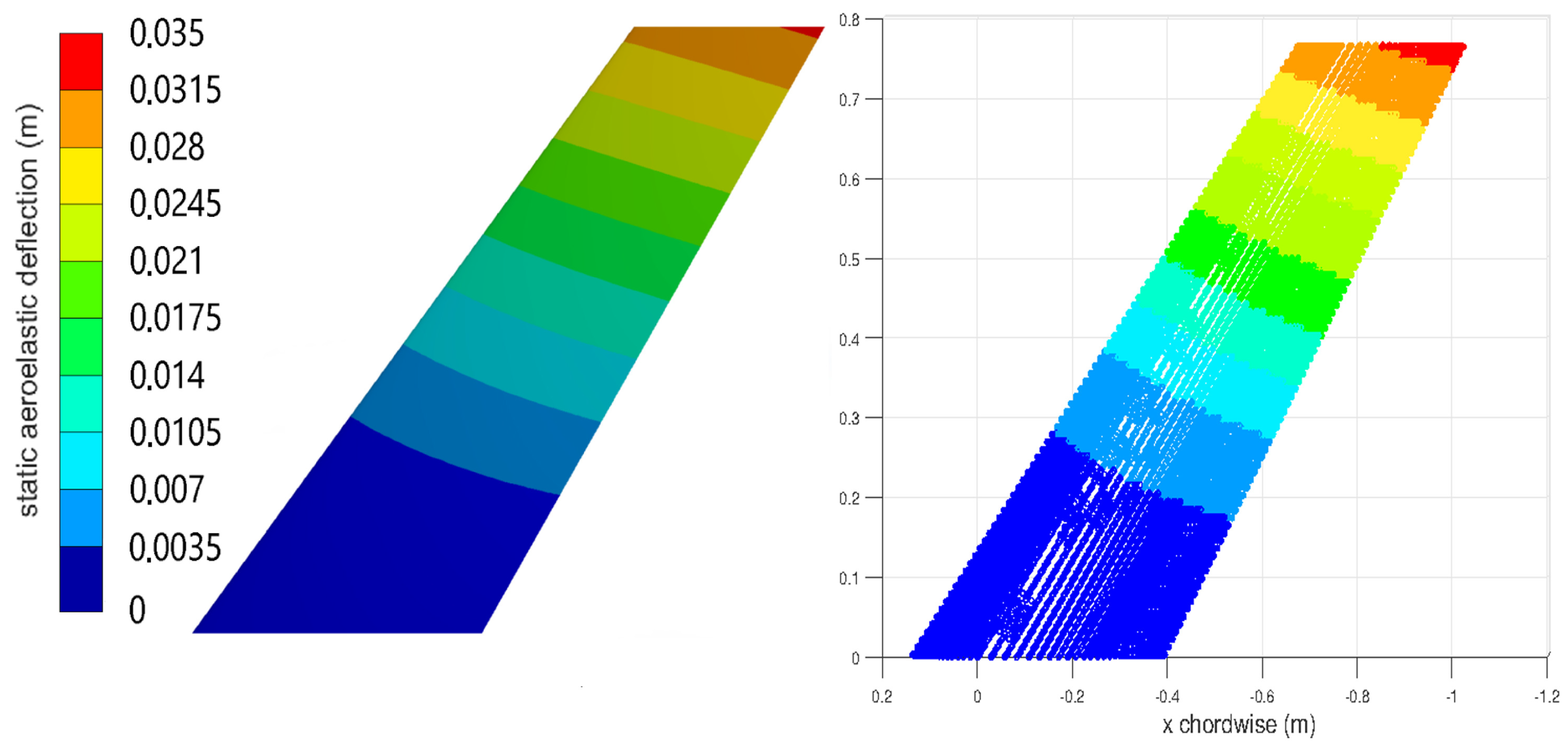
It is evident from the numerical results presented in
Figure 10,
Figure 11,
Figure 12 and
Figure 13 that both the coupled staggered and the critically damped reduced order model (ROM) solution compares well to the investigations in [
24].
Due to its back-swept geometry, the AGARD wing exhibits a restoring bending-torsion coupling, and as the wing is bent upwards, the aeroelastic twist tends to reduce the effective angle of attack with respect to the flow. This is captured in the preceding solutions by the displacements of the leading and trailing edge.
In both cases, the displacement of the trailing edge is higher than that of the leading edge, corresponding to an aeroelastic twist angle that reduces the effective angle of attack.
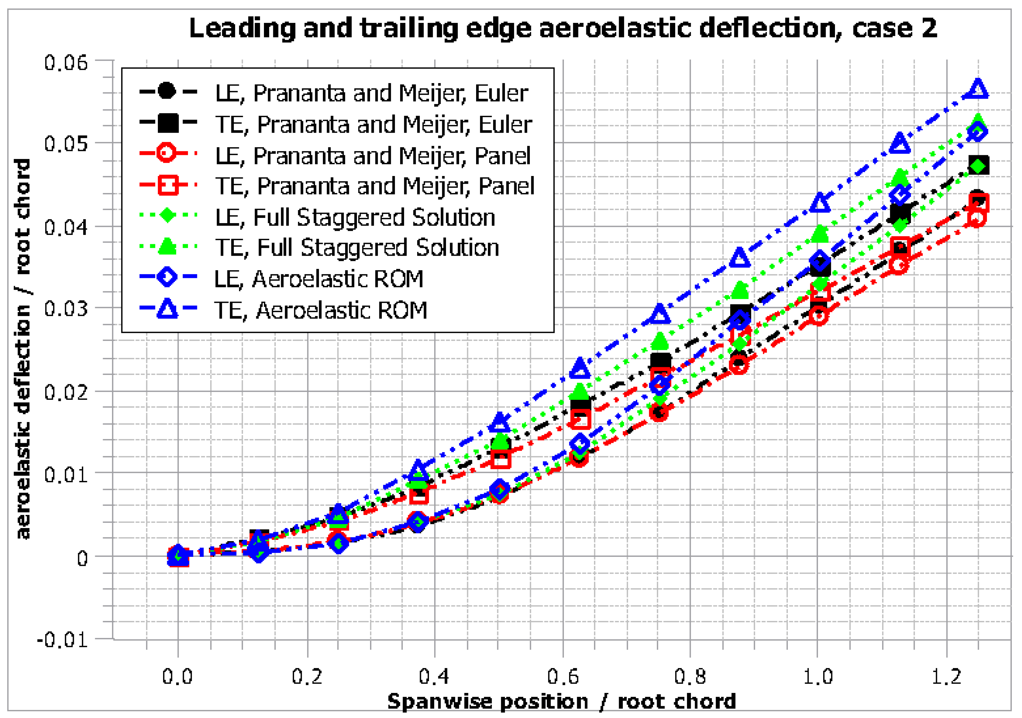
It can also be established by comparing
Figure 11 and
Figure 13 that for a Mach number of 0.45, the deformation trends for all solutions show very good agreement, whereas for Mach 0.96, and thus near the transonic region, several differences between the solutions obtained by high fidelity and low fidelity aerodynamics can be pinpointed.
Not only is the total deformation for both the leading and trailing edge higher for the higher fidelity solutions compared to the panel method solutions, but also, the distance between the two displacement curves is noticeably larger.
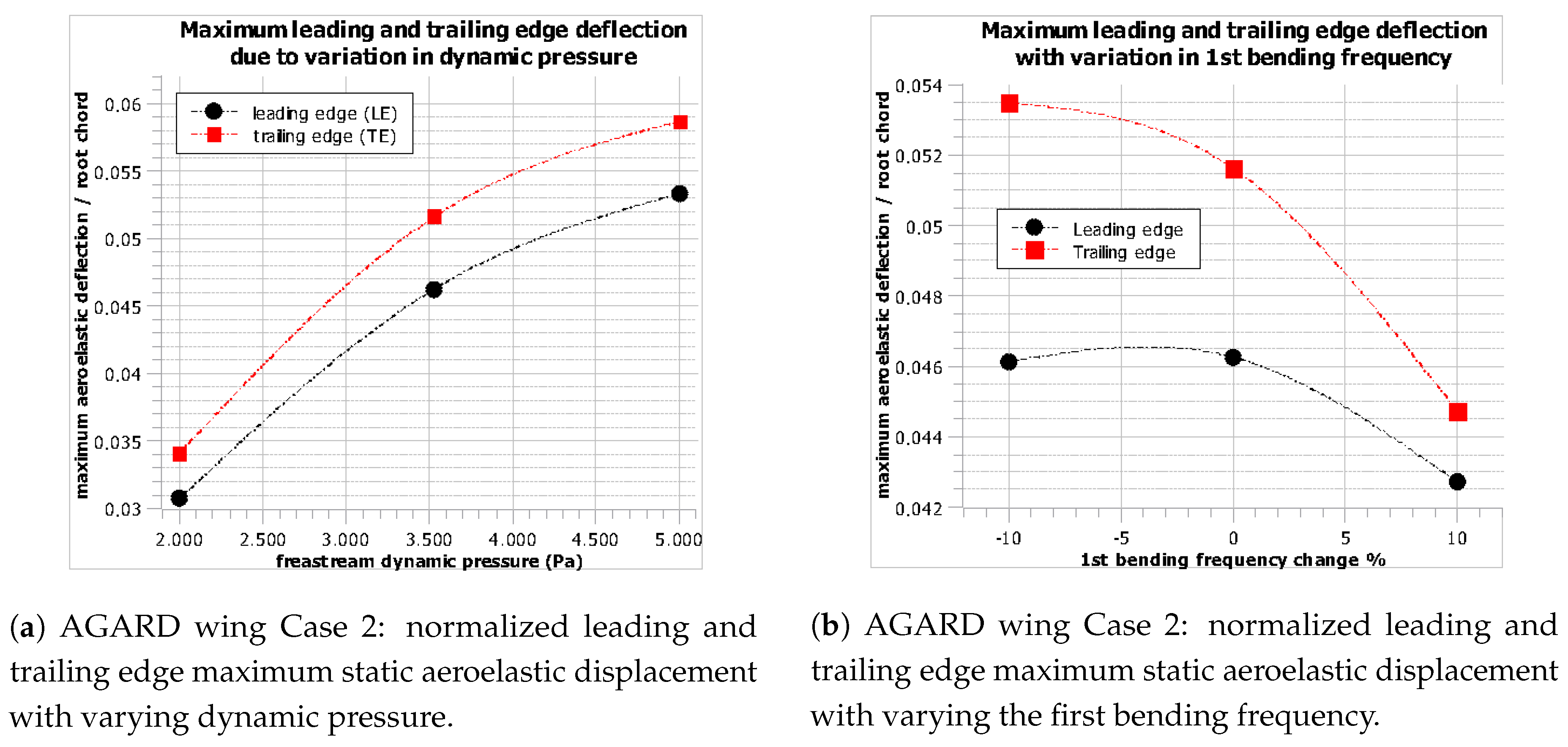
A significant advantage of using a reduced order model approach is the ability to model variations in dynamic pressure and factors like natural frequencies and damping ratios around a Mach number without the need to rerun the full solution.
The static aeroelastic deflection of the first case of
Table 4 due to variations in dynamic pressure and the first bending frequency are subsequently provided as an example of the flexibility gained by using the ROM approach.
Several important conclusions can be drawn from
Figure 14. Since as already mentioned, the AGARD 445.6 wing has a back-swept configuration, the resulting bending-torsion coupling tends to counteract the aeroelastic twist, therefore also limiting the aeroelastic deformation increase with increasing dynamic pressure in
Figure 14a.
Similarly, if the first bending frequency is increased while the rest remain unchanged, the stiffer behavior of the wing is evident in
Figure 14b. However, this increase in frequency corresponds to a smaller period; thus, it contributes less energy relative to the other mode shapes for the same time. Because the convergent bending-torsion coupling of the wing is mainly captured by the first bending mode shape, the restoring effect (evidenced by the higher aeroelastic displacement at the trailing edge compared to the leading edge) is at the same time reduced, as captured in
Figure 14b.
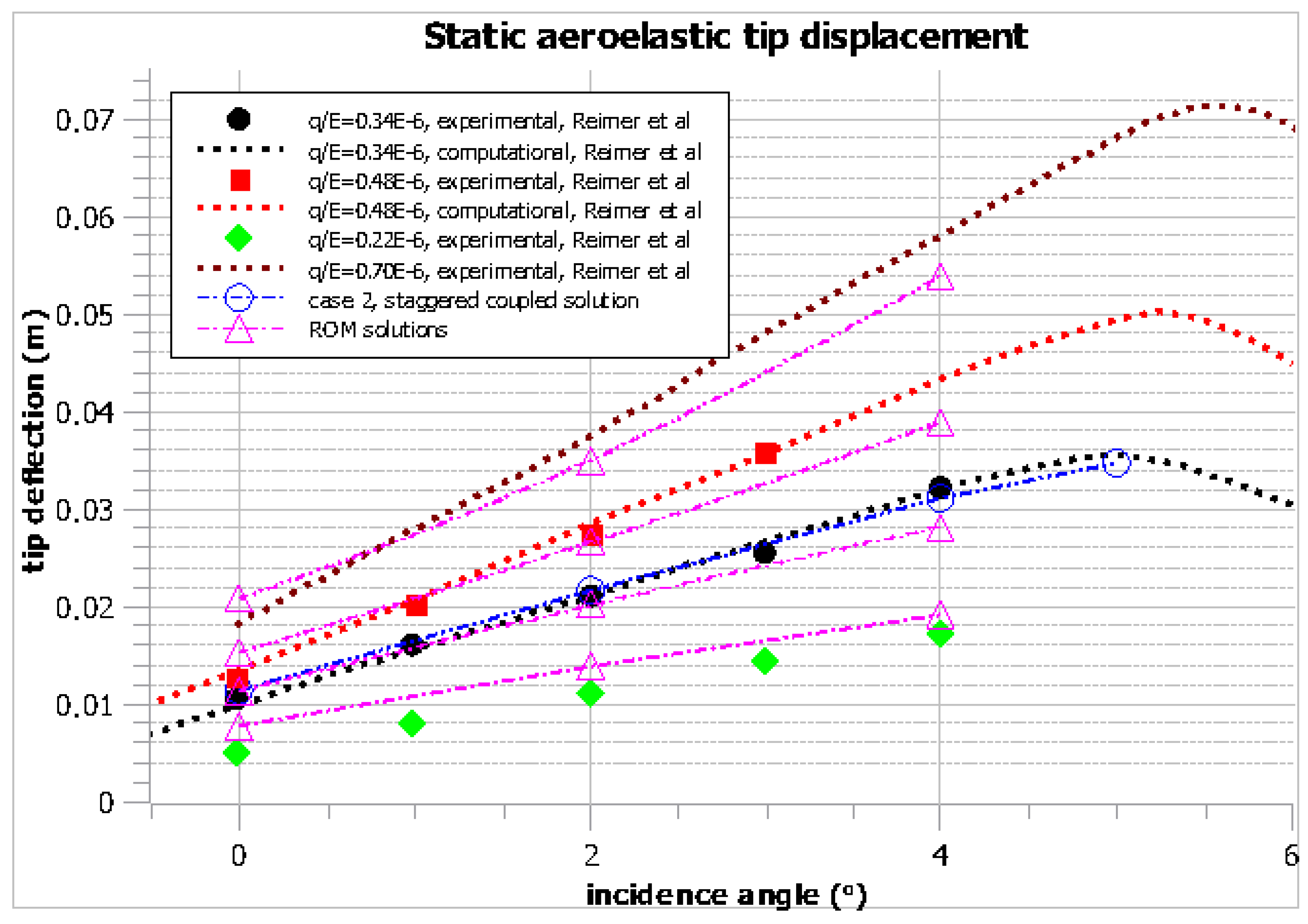
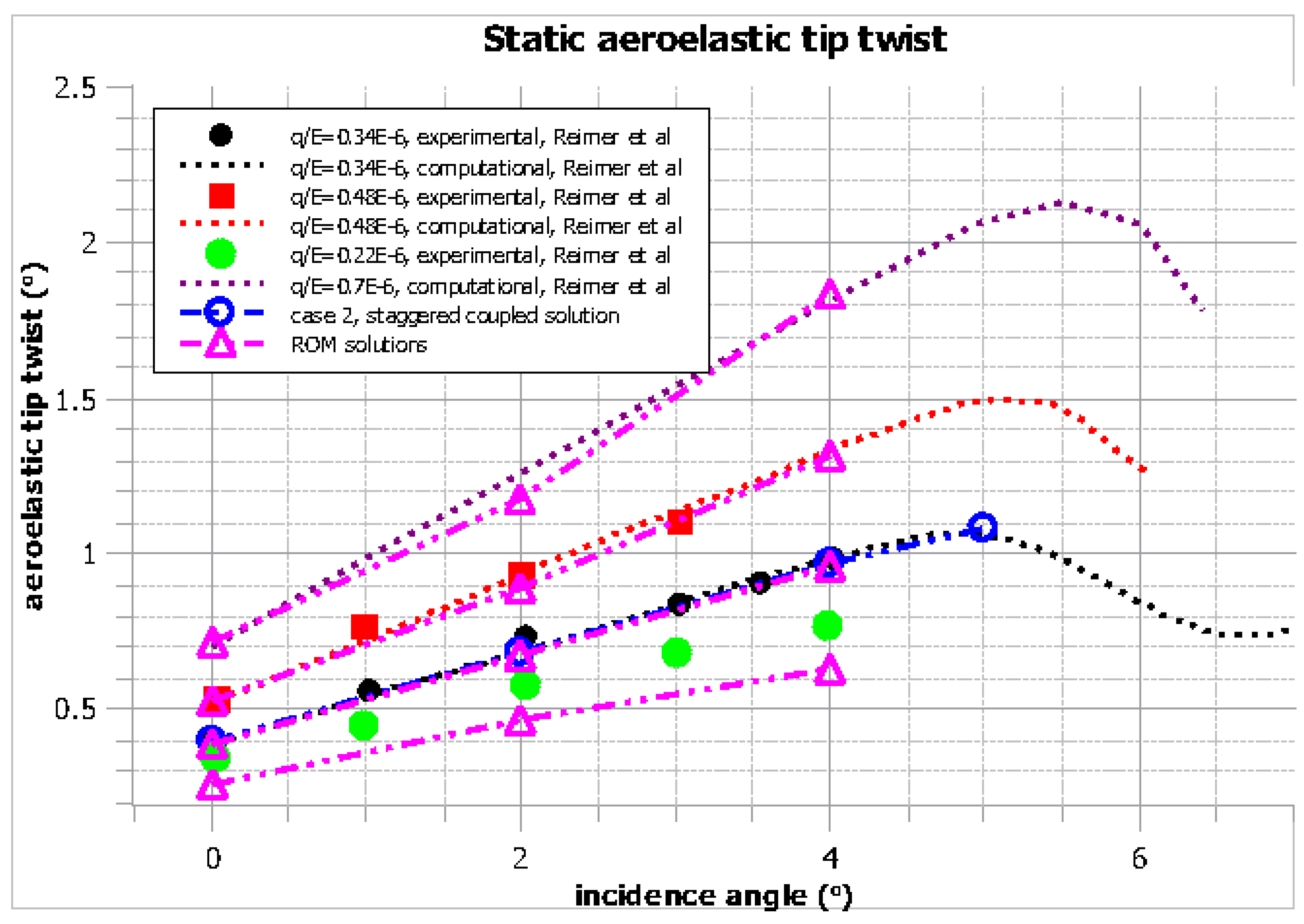
3.3. HiReNASD Wing Analysis
The static aeroelastic deflection and twist angle for the HiReNASD wing configuration are presented and compared with the numerical and experimental data from [
21]. The wing geometry, material properties, and wind tunnel test envelope were obtained from [
27].
The parameters for the wing material and the computational test envelope are given below in
Table 5 and
Table 6. A comparison of the structural mode shapes and frequencies with [
21] is given in
Table A6.
The solution to Case 2 was derived using both the full staggered and ROM approaches. Additionally, due to the ability of the ROM to remain valid for variations of dynamic pressure, the solutions to Cases 1, 2, and 4 were readily obtained by using the same sample data and thus with minimal additional computational cost.
The eigenmode frequencies (
Table A6) exhibit some deviation from the experimental results in [
28], but show good agreement with the ones obtained in [
21] for a similar finite element model and supports. The most likely cause of this discrepancy is the omission of the mounting device and extra mass due to cabling and instrumentation in the present finite element analysis (FEA) model that was based on the one from [
27].
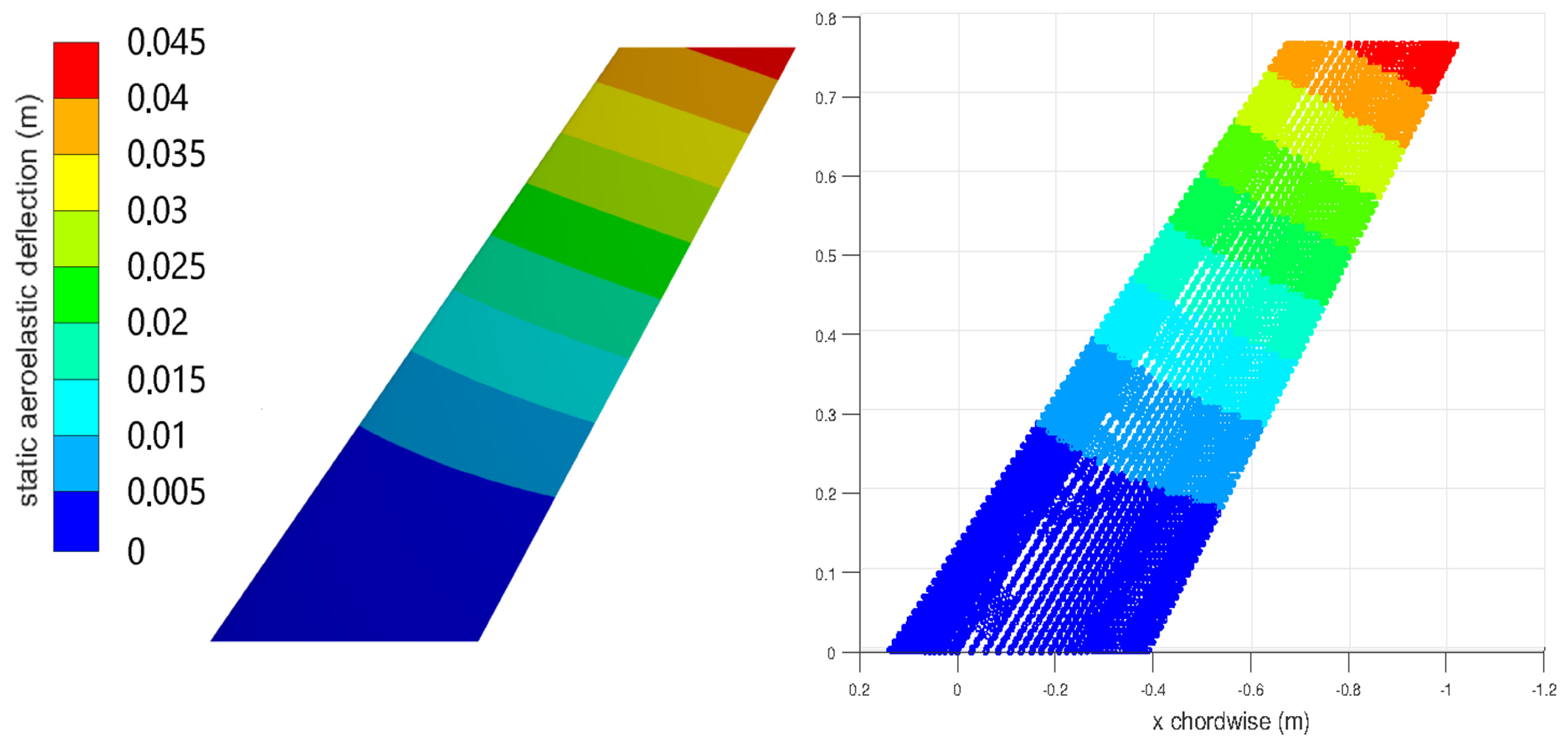
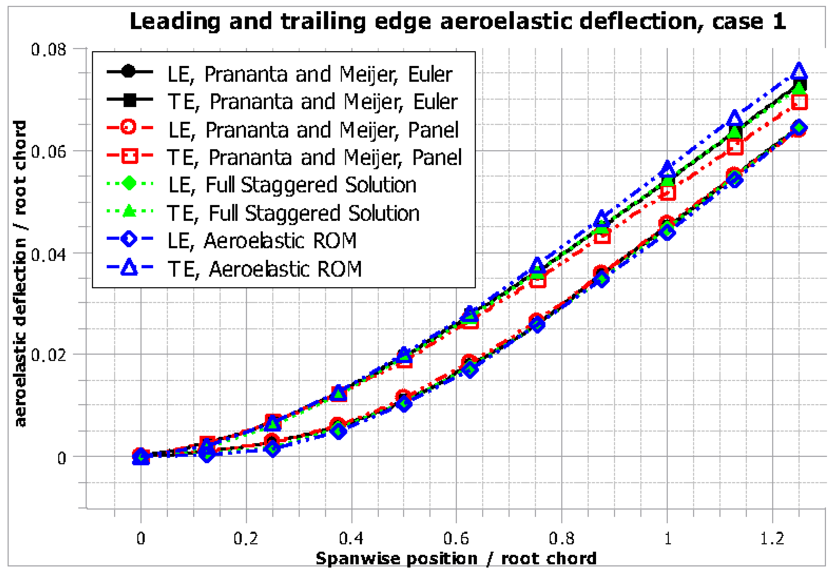
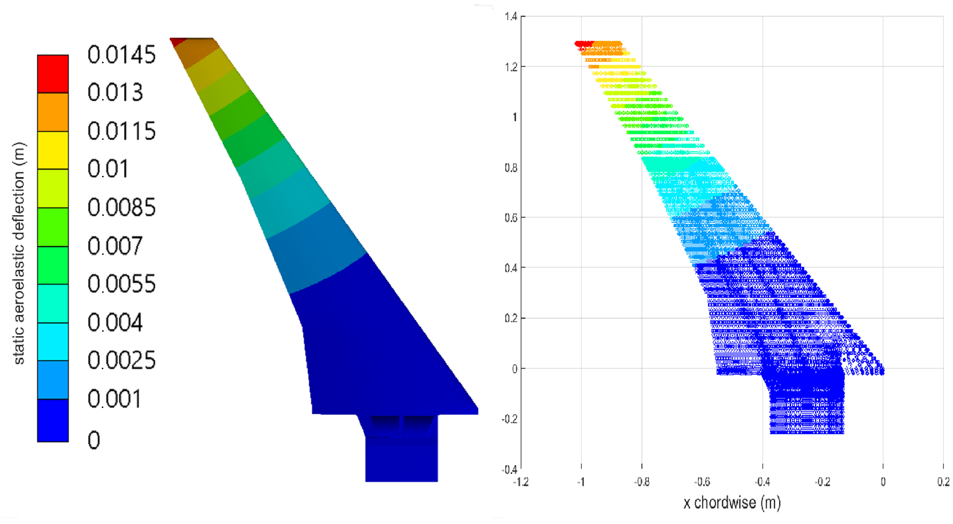
Nevertheless, the results presented in
Figure 15 (deflection contours) and in
Figure 16 and
Figure 17 (tip leading and trailing edge deflections) agree well with the computational and experimental ones [
21].
For a q/E of 0.34
, good agreement is shown between the computational results of Reimer et al. [
21], the staggered coupled solutions performed in the present study, and the reduced order model (ROM) solution.
Likewise, reasonable agreement between the computational results of [
21] and the ROM solutions exists for the other dynamic pressure values.
3.4. Computational Cost Analysis
The computational costs corresponding to a single static and dynamic aeroelastic staggered coupled solution and the construction and execution of a four mode shape ROM for the current computational setup of the AGARD 445.6 wing presented below emphasize the strong argument in favor of using a reduced order modeling approach. The computational cost is presented as minutes expended for each task in an ≈200,000 MIPS processor in
Table 7.


