Article

Implementation and Hardware-In-The-Loop Simulation of a Magnetic Detumbling and Pointing Control Based on Three-Axis Magnetometer Data

by
M. Salim Farissi
,
Stefano Carletta
*,†,
Augusto Nascetti
and
Paolo Teofilatto
School of Aerospace Engineering, Sapienza University of Rome, 00138 Rome, Italy
*
Author to whom correspondence should be addressed.
These authors contributed equally to this work.
Aerospace 2019, 6(12), 133; https://doi.org/10.3390/aerospace6120133
Submission received: 31 October 2019 / Revised: 30 November 2019 / Accepted: 6 December 2019 / Published: 11 December 2019
(This article belongs to the Special Issue Verification Approaches for Nano- and Micro-Satellites)

Abstract

:
The subject of this work is the implementation and experimental testing of a purely magnetic attitude control strategy, which can provide stabilization after the deployment and pointing of the spacecraft without any attitude information. In particular, the control produces the detumbling of the satellite and leads it to a desired attitude with respect to the direction of the Earth magnetic field, based on the only information provided by a three-axis magnetometer. The system is meant to be used as a backup solution, in case of failure of the primary strategy and is designed considering the constraints set on time of operations, power consumption, and peak electric current for a typical CubeSat mission. The detumbling and pointing algorithms are implemented on the FPGA core of a CubeSat on-board computer and tested by Hardware-in-the-loop simulations. The simulation setup includes a Helmholtz cage, recreating the magnetic environment along the orbit, the on-board computer, a MEMS three-axis magnetometer and Simulink software, on which the attitude dynamics is propagated. Test on the real system can provide useful information to select the parameters of the control, such as the gains, to estimate the limits of the system, the time of operations and prevent failures.

1. Introduction

The Attitude Determination and Control System (ADCS) plays a vital role in spacecraft mission operations. It provides information regarding the spacecraft orientation (or attitude) in space and produces the control action necessary to modify its attitude, according to some input or prescribed control laws. The successful development of an ADCS starts from concept design and should include numerical and experimental validation of the algorithms and hardware, to confirm its performance and robustness in different operative scenarios.
During the last decades, the introduction of the CubeSat standard gathered the attention of universities and small companies, because of the possibility to develop satellites and space missions with a limited budget [1,2]. The ADCS implemented under such a budget constraint are typically based on low-cost Components Off-The-Shelf (COTS), thus sensors and devices which are not tailored for space applications and novel system architecture. For this reason, experimental testing should represent an essential part of the development process.
It is known from statistical analysis that the majority of CubeSat mission end in failure right after the deployment. According to [3] the impact of ADCS failure on the number of “dead on arrival” CubeSats seems to be marginal, but a system-oriented interpretation of the results provides a clearer view on the issue. In fact, if ADCS failures may not affect the functionality of the other on-board systems, they do not allow those systems to operate in the design conditions, jeopardizing the mission, eventually causing its failure.
In the recent past, some strategies for low-cost Software-in-the-loop (SiL) or even Hardware-in-the-loop (HiL) testing of ADCS have been proposed. In SiL testing, the space environment, the satellite attitude dynamics, and the ADCS devices are all simulated, therefore the accuracy of the result depends on that of the model used for each one of the mentioned elements of the loop [4,5,6]. SiL simulations can be successfully applied to verify the ADCS system architecture and algorithms and are less complex than HiL simulations, in which the real attitude sensors and actuators are used, allowing a more accurate estimation of the ADCS performance. To adequately test the mentioned ADCS devices, some crucial features of the space environment must be recreated on-ground by the HiL setup.
Some HiL setup include a Helmholtz cage [7,8,9], a device capable of reproducing the geomagnetic field vector on the satellite during its orbital motion, allowing the use of real magnetometers in the simulation loop. Spherical air-bearing testbeds are used to recreate the microgravity conditions [10,11,12], necessary to simulate the spacecraft attitude dynamics under the control of attitude actuators [13,14,15,16,17,18].
In this work, we propose the design of a purely magnetic ADCS, allowing CubeSat detumbling and pointing based on the only measurement data from a MEMS three-axis magnetometer. The system is developed considering constraints on time of operations, power consumption, and peak electric current set by common CubeSat on-board systems.
The ADCS algorithms are designed to be implemented on the FPGA core of the CubeSat On-Board-Computer (OBC) ABACUS, designed by the School of Aerospace Engineering (SIA) and successfully flight proven [19]. The algorithms and part of the ADCS hardware (OBC and magnetometer) are tested by HiL simulations, using the Helmholtz cage available at SIA Flight Mechanics Laboratory “Michele D. Sirinian”. The configuration of the facility and calibration of the magnetometer are also part of this work and will be discussed in detail.
The manuscript is organized as follows, the background on spacecraft attitude dynamics and magnetic control is provided in Section 2. In Section 3 the configuration and calibration of the test hardware is presented, indicating the solutions selected and the performance of the experimental setup. The results for some selected test cases are presented and commented in Section 4, producing a preliminary characterization of the ADCS. Final comments are reported in the Conclusions section.

2. Spacecraft Attitude Dynamics and Magnetic Attitude Control

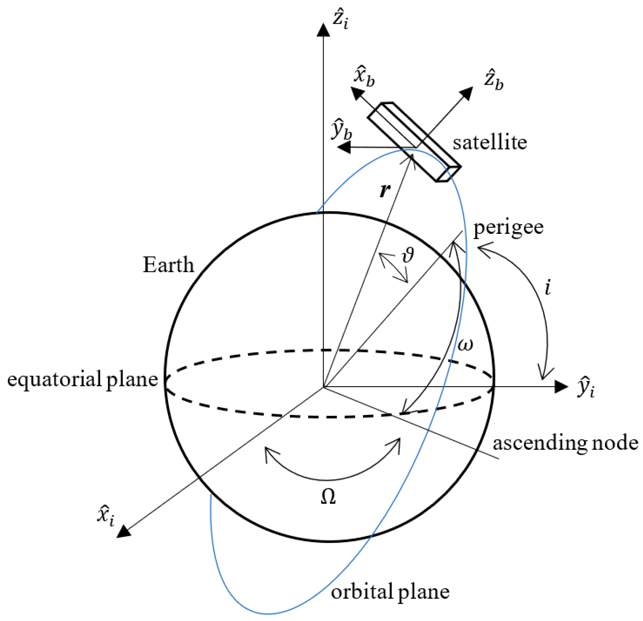
2.1. Attitude Dynamics

Attitude dynamics is modelled considering the spacecraft as a rigid body which is free to rotate about its center of mass. The principal moments of inertia are used to define the body frame F b = [ x ^ b , y ^ b , z ^ b ] which rotates rigidly with the spacecraft. An inertial reference frame F i = [ x ^ i , y ^ i , z ^ i ] is identified as well, here selected as the GeoCentric Inertial frame (GCI) [20], so that the Euler angles ( φ , θ ,   ψ ) transforming F b into F i can be used to describe the spacecraft attitude. Furthermore, the angular velocity at which F b rotates with respect to F i represents the angular velocity of the spacecraft ω = [ ω x ω y ω z ] T . The two reference frames are sketched in Figure 1.
Based on this representation, the dynamic equations of attitude motion are represented by the following system [20]:
{ φ ˙ = ω x + sin φ tan θ ω y + cos φ tan θ ω z θ   ˙ = cos φ ω y sin φ ω z ψ ˙ = ( sin φ ω y cos φ   ω z ) cos θ { ω ˙ x = ( J y J z J x ) ω y ω z + τ c , x + τ d , x ω ˙ y = ( J z J x J y ) ω x ω z + τ c , y + τ d , y ω ˙ z = ( J x J y J z ) ω x ω y + τ c , z + τ d , z
where τc,i and τd,i are, respectively, the components of the control and disturbance torques acting on the satellite, described in detail in the following subsections.

2.2. Magnetic Attitude Control

In the ADCS developed here, the control torque is produced by the interaction between the geomagnetic field surrounding the spacecraft (Bb), measured by the three-axis magnetometer, and the magnetic dipole moment m = [ m x m y m z ] generated by the magnetic coils (or magnetorquers) installed on-board, representing the attitude control devices. The torque can be expressed by the following equation
τ c = m × B b
In particular, the system consists of three mutually orthogonal magnetorquers, each one generating a magnetic dipole moment mi along one of the directions of F b (see Figure 2)
m i = N i A i I i        i = x , y , z
where Ni and Ai are, respectively, the number of turns and the mean area of the coil along orthogonal to the i-th body-frame direction, and Ii is the electric current in the wire of the coil.
The magnetorquers are controlled by regulating the intensity of I, which can be determined based on that of the magnetic dipole moment necessary to produce the desired attitude motion. Two control laws were implemented, one producing the spacecraft detumbling, or stabilization after deployment, and one setting the spacecraft attitude to some prescribed angle with respect the geomagnetic field vector, hereafter referred to as B-pointing.
Detumbling control has long been studied and is simply described by the following equation for the magnetic dipole moment [21]:
m d = K d   B b ˙
where Kd is the control gain and B b ˙ is the time derivative of the geomagnetic field measured by the on-board magnetometer. Indicating with fk the sampling frequency of the ADCS and with k the sample, the value of the derivative can be calculated as follows:
B b ˙ = f k ( B b ( k ) B b ( k 1 ) )
B-pointing control represents an adaptation of the nadir-pointing control already implemented on TigriSat, a 3U CubeSat launched by the SIA in 2014 [22]:
m p = K p B b ×   ( r ^ × B ^ b )
where Kp is the control gain, r ^ is the unit vector representing the target attitude of the spacecraft and B ^ b is the direction of Bb. For a general case, r ^ should be provided by the attitude determination segment of the ADCS, which is not examined here. In fact, the aim of the proposed solution is that of representing an effective and reliable alternative to be activated when attitude determination is not available. In such a scenario, r ^ will be set equal to a prescribed direction in F b . The following two cases are examined in Section 4:
(a)
r ^ = [ 1   0   0 ] , producing x ^ b in the direction of Bb;
(b)
r ^ = [ 0.5 2   0.5 2   0 ] , setting y ^ b and z ^ b to an angle of 45 deg with respect to Bb.
Since a three-axis magnetometer can only resolve two out of three attitude angles, the B-pointing algorithm can control the spacecraft attitude along one (a) or two (b) directions at most. Considering for instance the case (b), the only attitude information available on third axis ( x ^ b ) is that it will always lay on a plane orthogonal to Bb. This result can be easily extended to case (a). It is worth to highlight that similar configurations produce a predictable attitude motion of the satellite which, in case of failure of the primary attitude determination devices, improving the survivability of the mission and allowing to implement magnetometer-only attitude estimation strategies [23,24,25,26,27,28,29,30,31].
Equations (4) and (6) represent the control laws of the ADCS, producing the total magnetic dipole moment given below:
m = m d + m p
Based on Equations (4), (6), and (7), the value of the electric current in the magnetorquers can be determined once fixed the parameters N = 400 and A = 9.03 × 10⁻³ m2 for all the coils, which have been selected in order to limit the power usage to P m a x = 250   mW at a supply voltage of V d r i v e = 3   V . It follows that the limit value for the current is I m a x = 83   mA , therefore the maximum value for the dipole moment which can be generated by each magnetorquer can be calculated from Equation (3) and is equal to m i m a x = 0.3   Am 2 .

2.3. Disturbance Torques

During the orbital motion of the satellite, a variety of external torque, beside the control one, act on it, producing a perturbation on the controlled attitude motion. The most relevant ones have been considered, caused by residual dipole moment ( τ m ) , gravity gradient ( τ g ) , and atmospheric drag ( τ a ) . The total disturbance torque is calculated as follows
τ d = τ m + τ g + τ a

2.3.1. Residual Dipole Moment Torque

The presence of magnetic materials or the electric currents in on-board electric devices can produce a residual magnetic dipole moment m m on the satellite [32,33]. The interaction of m m with the geomagnetic field B b produces a torque on the satellite, which can be evaluated by Equation (2)
τ m = m m × B b
The magnitude and direction of m m depend on the final configuration of the satellite, therefore they cannot be determined a-priori and a guessed value should be considered as long as the final configuration of the satellite is not defined, to verify the effectiveness of the control algorithms also in presence of such a perturbation. For the HiL simulations performed in Section 4, the magnitude | m m | = 0.1   Am 2 is selected, which is one order of magnitude higher than the values measured for similar CubeSat configurations [33,34], definitely representing a worst-case scenario.

2.3.2. Gravity Gradient Torque

Satellite with an unsymmetrical mass distribution are subject to gravitational torque, produced by the Earth’s gravitational field. The torque can be modelled as follows [20]:
τ g = 3 μ | r | 3   r ^ × [ J ] r ^
where r is the position vector of the satellite in GCI coordinates, μ = 3.986 × 10¹⁴ m3/s2 is the gravitational parameter of the Earth, [J] is the tensor of inertia of the satellite and r ^ = r / | r | . The value of | r | can be calculated from the polar equation for a Keplerian orbit:
| r | = a ( 1 e 2 ) 1 + e cos ϑ
where a and e indicate the semimajor axis and the eccentricity of the orbit and ϑ is the true anomaly. The components of r in the GCI frame can be calculated applying the following rotation matrix, transforming a vector in the orbital plane to the GCI one [20]:
[ R o , i ] = [ cos Ω cos ( ω + ϑ ) s i n Ω cos i sin ( ω + ϑ ) cos Ω sin ( ω + ϑ ) s i n Ω cos i cos ( ω + ϑ ) sin Ω sin i sin Ω cos ( ω + ϑ ) + cos Ω cos i sin ( ω + ϑ ) cos Ω cos i cos ( ω + ϑ ) s i n Ω sin ( ω + ϑ ) cos Ω sin i sin i sin ( ω + ϑ ) cos ( ω + ϑ ) sin i cos i ]
where Ω is the RAAN, ω is the argument of perigee and i is the inclination of the orbital plane. Based on matrix (12), r is defined by the transformation below:
r = [ R o , i ] [ | r | 0 0 ]

2.3.3. Aerodynamic Torque

Aerodynamic torque arises from the aerodynamic drag produced by the interaction of the satellite surfaces with the residual atmosphere at high altitude, which is represented by the following equation [35]:
D = 1 2 ρ S C D V 2   V ^
where ρ is the density of air, which can be modelled according to NRLMSISE-00 empirical model [36], S is the normal projection of the satellite area to the incident flow, CD is the drag coefficient of the satellite [37], and V is its orbital speed which can be determined as follows:
V = μ ( 2 | r | 1 a )
To calculate the aerodynamic torque, the unit vector V ^ must be expressed in F b , by applying the following coordinate transformation [20]:
V ^ = [ R i , b ] [ R o , i ] [ 0 1 0 ]
where the rotation matrix [ R i , b ] transforms F i to F b and is given below:
[ R o , i ] = [ cos ψ cos θ cos ϕ sin ψ + cos ψ sin ϕ sin θ sin ϕ sin p s i   cos ψ cos ϕ sin θ cos θ sin ψ cos ϕ cos ψ sin ψ sin ϕ sin θ cos ψ sin ϕ + cos ϕ sin ψ sin θ sin θ cos θ sin ϕ cos ϕ c o s θ ]
The expression for the aerodynamic torque in F b is reported below [35]:
τ a = l × D
where l is the arm of the torque, corresponding to the distance between the satellite center of mass and the aerodynamic center, which is the point where the aerodynamic force is applied. Estimating the aerodynamic center of the satellite requires dedicated analyses which are beyond the aim of this work [35], therefore for the HiL simulation a worst case was considered, setting l equal to the half-length of each side of the satellite.

3. Configuration of the Hardware-In-The-Loop Simulation Hardware

A primary goal of this work is to verify the performance of the ADCS in producing the control laws proposed in Section 2. To achieve this result, the experimental setup for HiL simulations is configured.

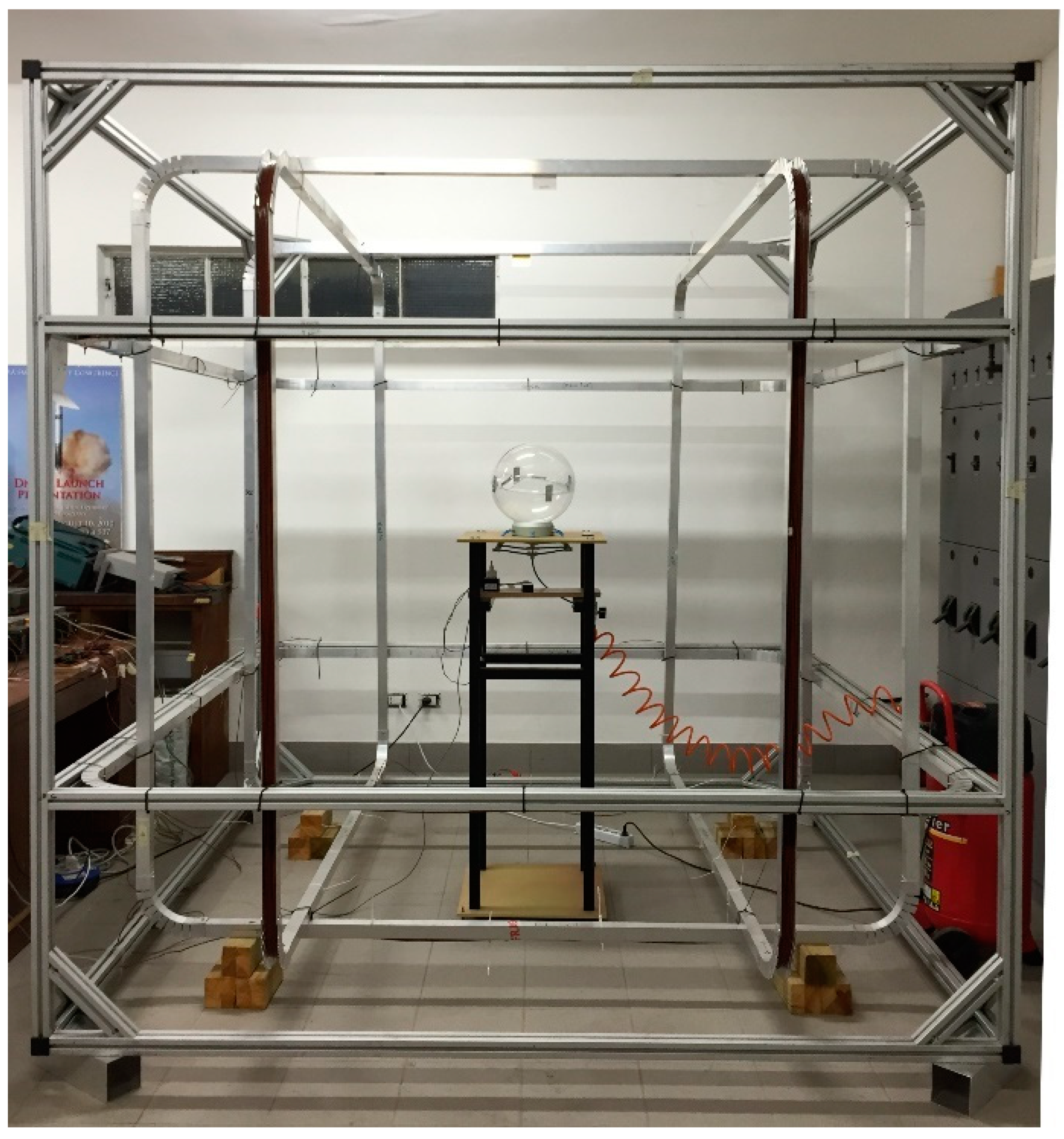
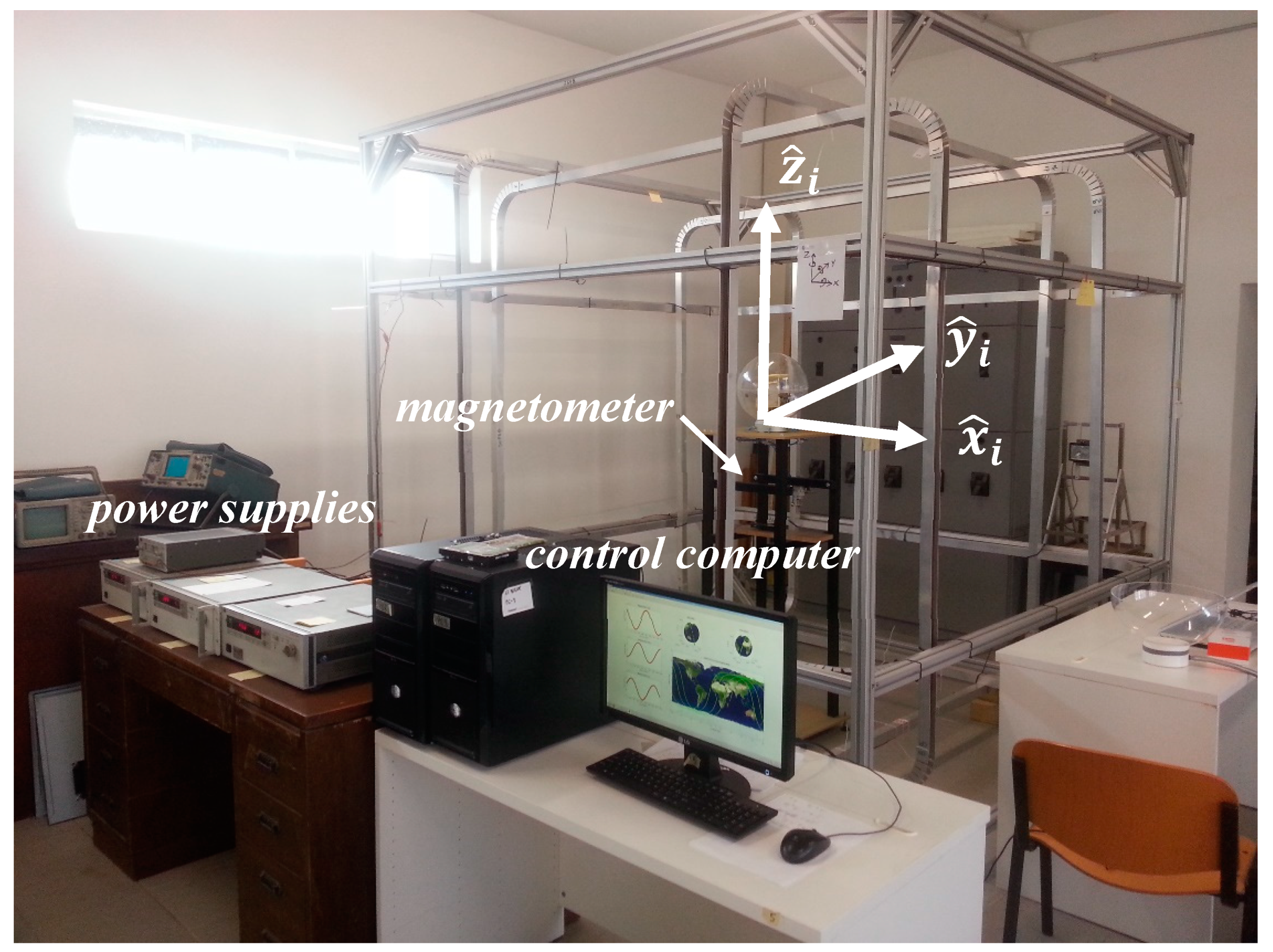
3.1. Helmholtz Cage Configuration

A 3 × 3 × 3 m3 Helmholtz cage is used to reproduce the geomagnetic field vector in F i at any orbital position of the spacecraft. The complete cage system is shown in Figure 3 and Figure 4. The magnetic field generated by the Helmholtz cage is uniform in a volume of 30 × 30 × 30 cm3 at the center of the cage. Each pair of coils produces a constant magnetic field orthogonal to their surface, whose magnitude can be estimated by the following approximated relation:
B i = 2 μ 0 N I i π l 2 ( 1 + β 2 ) 2 + β 2       i = x , y , z
where μ 0 is the permeability of free space, N = 54 and l = 1.24 m are, respectively, the number of turns and the half length of the side of the coils, β = 0.5445 is the ratio of the distance between the two coils and I is the electric current in the coils. The facility was designed to operate in the range ±2 × 10⁻⁴ T along each direction.
In addition to the Helmholtz cage, the system includes:
  • 3 power supplies, each one feeding one pair of coils, allowing the generation of a magnetic field vector with desired intensity and direction;
  • a control computer, on which the orbital motion of the satellite is simulated, based on the input orbital parameters, and the corresponding value of Bi for each position of the satellite is calculated in real-time, using the International Geomagnetic Reference Field (IGRF) model [38];
  • a calibrated three-axis magnetometer, measuring the magnetic field in the central and constant region of the Helmholtz cage.
All the mentioned elements form a closed-loop system which operates according to a control code implemented in Matlab. A Proportional Integral Derivative (PID) controller allows generating a magnetic field with an error in the range ±1 × 10⁷ T.
The list of the operations necessary to simulate the changing magnetic field during the orbital motion of the satellite is discussed hereafter. As a preliminary step, the desired orbital parameters are introduced in the control code, written in Matlab, along with the total time and the time step for the simulation. In particular, the time step can be selected in the frequency range 1–10 Hz, therefore allowing accelerated simulations up to a factor 10. It is worth noting that, to allow accelerated simulations, the sampling frequency of the ADCS must be compatible with that of the Helmholtz cage, as discussed in detail in Section 3.2. Corresponding to each time step, the following cycle is repeated:
  • the orbital propagator updates the true anomaly and calculates the position r of the satellite in F i , according to Equations (11)–(13);
  • using a Matlab routine, the longitude (Lo), latitude (La), and altitude (h) of the satellite at any r are calculated and the geomagnetic field Bi is computed from the IGRF model:
    { B i , x = 1 | r | V B L a B i , x = 1 | r | V B L a B i , x = 1 | r | V B L a
    where VB is the geomagnetic field scalar potential, reported below, whose parameters are defined in [38]:
    V B = R E n = 1 N m = 0 n ( R E | r | ) n + 1 [ g n m ( t ) cos ( m L o ) + h n m ( t ) sin ( m L o ) ] P n m cos L a
  • the value of the current to be provided to each pair of coils of the Helmholtz cage is calculated based on Equation (19);
  • the power supplies are activated from Matlab script, changing the magnetic field inside the cage, which is measured by the facility magnetometer Bm;
  • the reading from the magnetometer is sent to the control computer and the error between the desired and the measured value of the magnetic field is calculated, ϵ = B m B i ;
  • based on ϵ , a PID controller implemented in the code estimates the currents Ic_i to compensate the error;
  • the loop repeats until the end of the simulation.

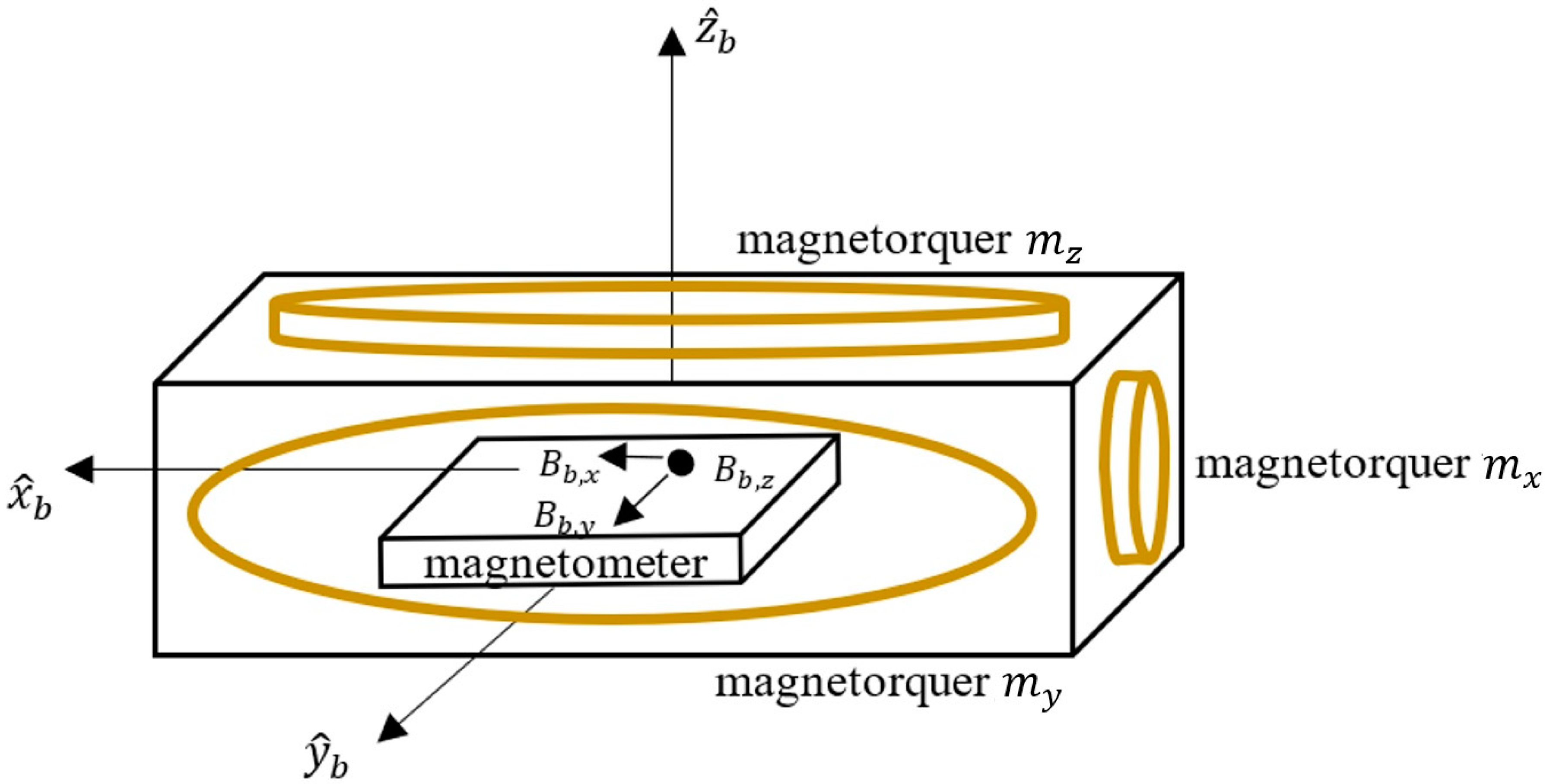
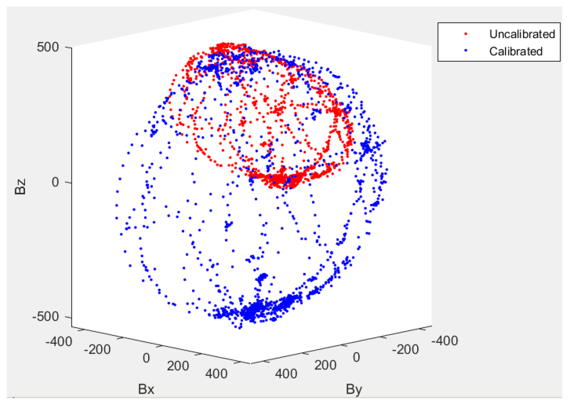
3.2. On-Board Magnetometer Configuration and Calibration

The ABACUS OBC is equipped with a Honeywell HMR2300 three-axis magnetometer, operating in the range ±1 × 10⁻⁴ T, with 12-bit measurement accuracy down to 1 × 10⁷ T and sampling frequency selectable between 10 and 154 Hz [19]. The three-axis magnetometer is a MEMS sensor, and can be therefore affected by some structural defects, related to the production technology, introducing non-isotropic measurement errors.
The goal of the calibration process is to characterize the magnetic sensors, so the satellite can process accurate values for the magnetic field strength and direction, under different modes of operation. Calibration is achieved by subjecting the three-axis magnetometer to a known magnetic field Bref, generated by means of the Helmholtz cage, calculating the measurement error and compensating it by least square fitting method.
The calibration starts calculating the offset Bo between the reference magnetic field Bref and the value read by the magnetometer Bm. Several measurements are repeated rotating the magnetometer about its center of mass. The offset values are stored and processed by ellipsoid fitting and linear least-squares method, which convert them into an ellipsoid representing the distribution in space of the offset. The semi-axes of the ellipsoid, indicated as Rx, Ry, and Rz, can then be collected in the matrix [T], defined as follows:
[ T ] = [ R x 0 0 0 R y 0 0 0 R z ]
After determining the 3 × 1 eigenvector v of [T], the compensated value B c can be calculated as follows:
B c = v [ T ] B ref v T B o
At the end of the calibration, the semi-axes calculated by the ellipsoid fitting method should be equal one the other. An example is reported in Figure 5, showing the comparison between the measurements before (red) and after (blue) the calibration of the OBC magnetometer.

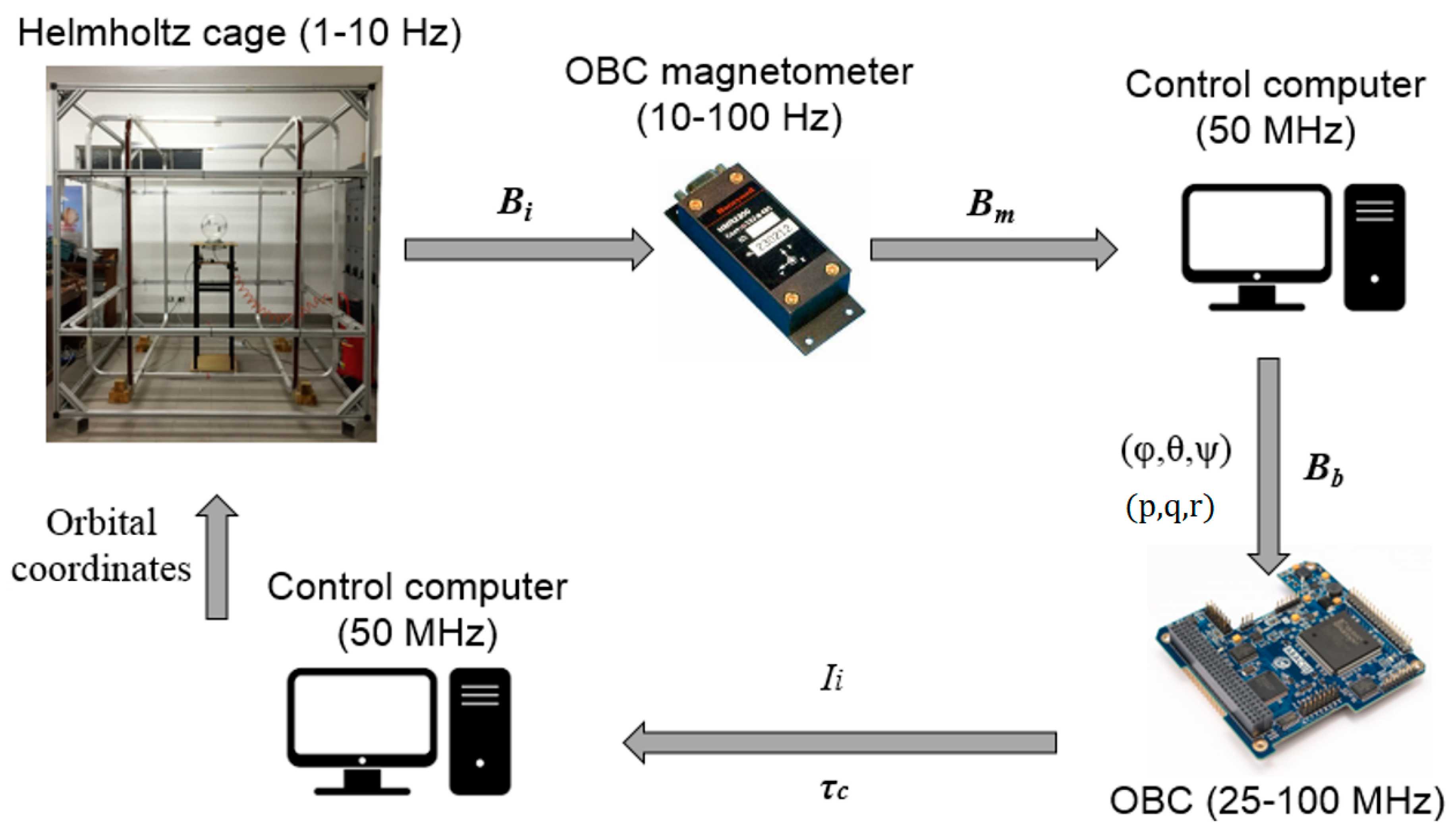
3.3. Hardware-In-The-Loop Platform Configuration

The HiL platform is configured as follows and represented in the block diagram in Figure 6:
  • Helmholtz cage system, generating Bi based on the estimates of the orbital propagator running on the facility control computer;
  • on-board three-axis magnetometer (integrated to the OBC), measuring the magnetic field generated by the Helmholtz cage;
  • OBC, on which the control algorithms are implemented, producing the driving current to the magnetorquer and the magnetic control torque;
  • control computer, propagating the orbital motion to calculate Bi, calculating the disturbance torques, and integrating the attitude dynamics equations to determine the Euler angles and angular rates.
Attitude dynamics is simulated using Simulink fixed step ode8 integrator. The integration time for the software is synchronized with that of the HiL simulations, which was selected to be 10 times faster than real time. This corresponds to an operating frequency of 10 Hz for the Helmholtz cage, therefore, to avoid loss of information, the sampling frequency of the OBC magnetometer is set to 100 Hz.
It is worth noting that, since the attitude motion of the spacecraft is just simulated, the magnetometer will not read values of the geomagnetic field in F b , but in F i instead. Therefore, the coordinate transformation from Bi to Bb is performed in Simulink, after calculating the Euler angles (φ,θ,ψ) from the integration of system (1) and based on the input (Bi) from the OBC three-axis magnetometer. The measured value of Bb is then processed by the OBC to calculate the magnetic dipole moment required to perform the detumbling and/or B-pointing control, according to Equations (4) and (6). Once determined m, the value of the current is calculated from the inverse of Equation (3) and sent to the power board, which feeds the magnetorquers. To avoid that the magnetic field generated by the magnetorquer interferes with the measurements of the magnetometer, a duty cycle is defined, such that the magnetorquers are activated only for the 90% of the cycle and the remaining 10% is dedicated to the measurements by the magnetometer. Once again, because of the simulated attitude dynamics, the values of the currents are converted to the torque components into the Simulink model, as they are needed to integrate system (1).

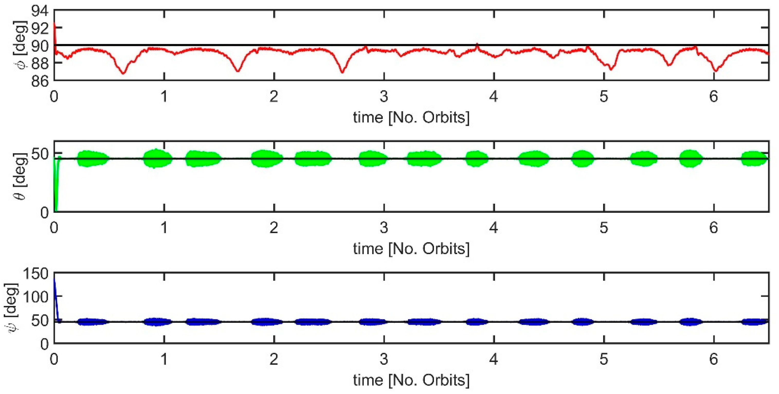
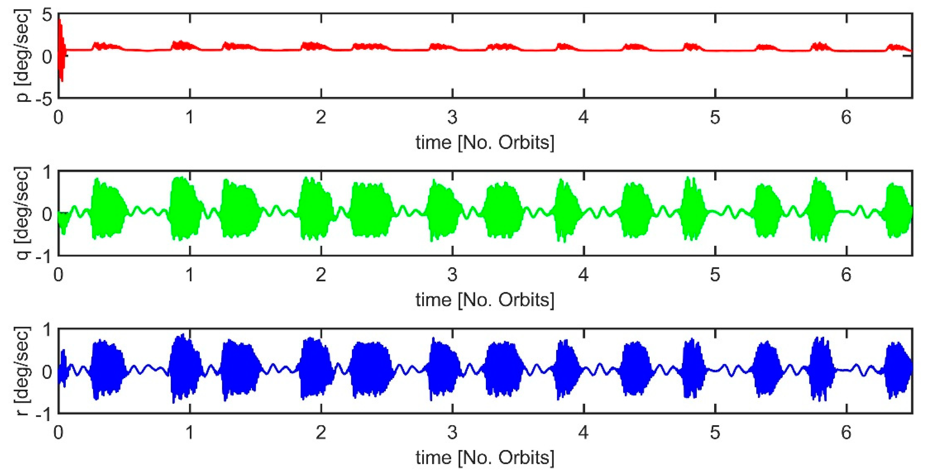
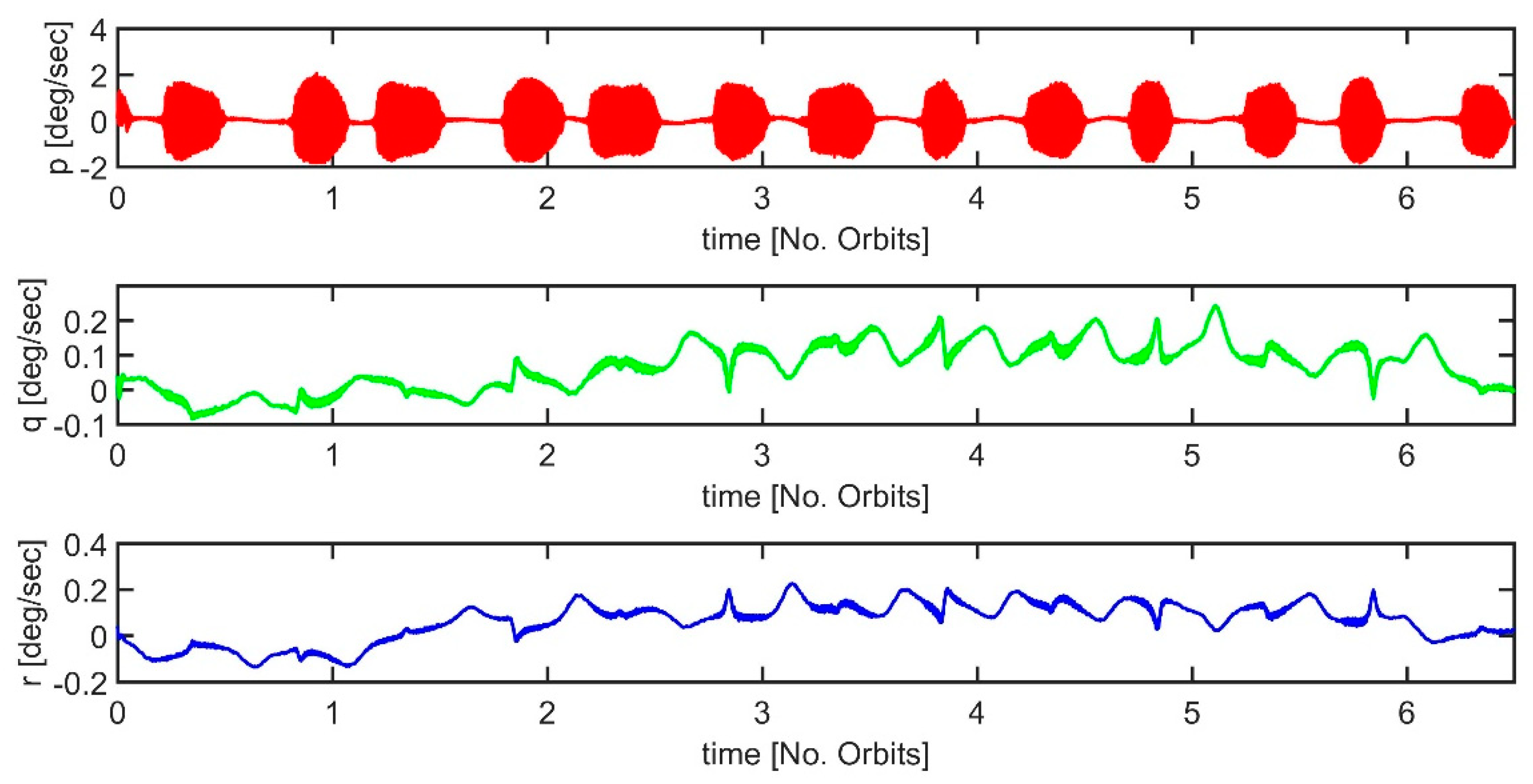
4. Hardware-In-The-Loop Simulations

The detumbling and B-pointing algorithms were tested through HiL simulations, considering the orbital and design parameters for TigriSat, a 3U CubeSat designed and launched by SIA in 2014 and equipped with ABACUS. The characteristic parameters of the disturbance torque were selected to represent realistic worst cases and are indicated, together with the previous ones, in Table 1.
The results of three Test Cases (TC) are presented and discussed. In TC1 the detumbling control is verified setting to zero the gain for the pointing control, and assuming the initial angular rates at the deployment reported in Table 2. The detumbling is simulated for a total time corresponding to 1.5 orbital periods and the satellite state (position, velocities and angular rates) at the end of the detumbling phase is assumed as the initial condition for TC2 and TC3, in which pointing control is tested for two different values of the target attitude. The simulation parameters are collected in Table 2.
The time behavior of the angular rates is reported in Figure 7, showing the effectiveness of the control law (4) in producing the desired decrease of the angular rates along all the three directions. The mean value of the angular rates in the last 300 s (5%) of the detumbling phase is equal to ω = [ 0.085 0.041 0.042 ]   deg / sec .
Figure 8 and Figure 9 show the behavior in time of the Euler angles for TC2 and TC3. The HiL simulations are performed for a total of 6.5 orbital periods, considering for the initial conditions the final state corresponding to TC1. It can be noticed that for both the test cases, the Euler angles settle about the target value (see r ^ in Table 2). The minimum, maximum, and mean error corresponding over the last orbital period are reported in Table 3. It is worth noting that the minimum error here represents the negative error with maximum absolute value.
The values reported in Table 3 indicate that, despite the presence of perturbation torque, pointing control (6) is effective within an accuracy of, approximately ±10 deg on average and ±20 deg considering the maximum values. In particular, TC2 seems to be more challenging than TC3. In fact, for r ^ = [ 1   0   0 ] the system will drive the satellite if the magnetic field measured along y ^ b and z ^ b is not null, or equivalently if the component measured along x ^ b is equal to the magnitude of the magnetic field. Clearly, any component measured at time t can never exceed the magnitude of the magnetic field   | B b ( t ) | , then the control shows aperiodic behavior, limiting its accuracy. Differently, when the magnitude of the magnetic field is “shared” by two or more components, such as r ^ = [ 0   0.5 2   0.5 2 ] , then the component measured along the directions y ^ b and z ^ b can, at different times, exceed the target value 0.5 2   | B b ( t ) | and the behavior of the control is oscillatory about the target value. This can be proved by observing that the maximum and minimum error for TC3 are (almost) equally distributed about the mean value. This is not the case for TC2, in which the maximum value is much larger in magnitude than the minimum one.
It is worth noting that the maximum error on the Euler angles is measured when the satellite crosses the poles. In this region the direction of the geomagnetic field vector changes suddenly and in particular Bi points towards the North magnetic pole when the latitude is slightly lower than 90 deg and outwards from the pole when the latitude is higher than 90 deg (similarly in the neighborhood of the South pole). According to Equation (6), a marked variation of the direction of Bi produces a high torque onto the satellite, increasing its angular rates, therefore longer time is required to damp the angular oscillations and reduce their amplitude about the target attitude.
Figure 10 and Figure 11 show the angular rates for TC2 and TC3. It can be noticed that when the pointing phase starts, the angular rates increase, with higher intensity on the axes which are controlled to the target attitude (i.e., x ^ b for TC2 and y ^ b and z ^ b for TC3). This is a consequence of the control torque arising from mp.

5. Discussion

In this section, some relevant features of the attitude control system, inferred from the HiL simulations, are briefly outlined:
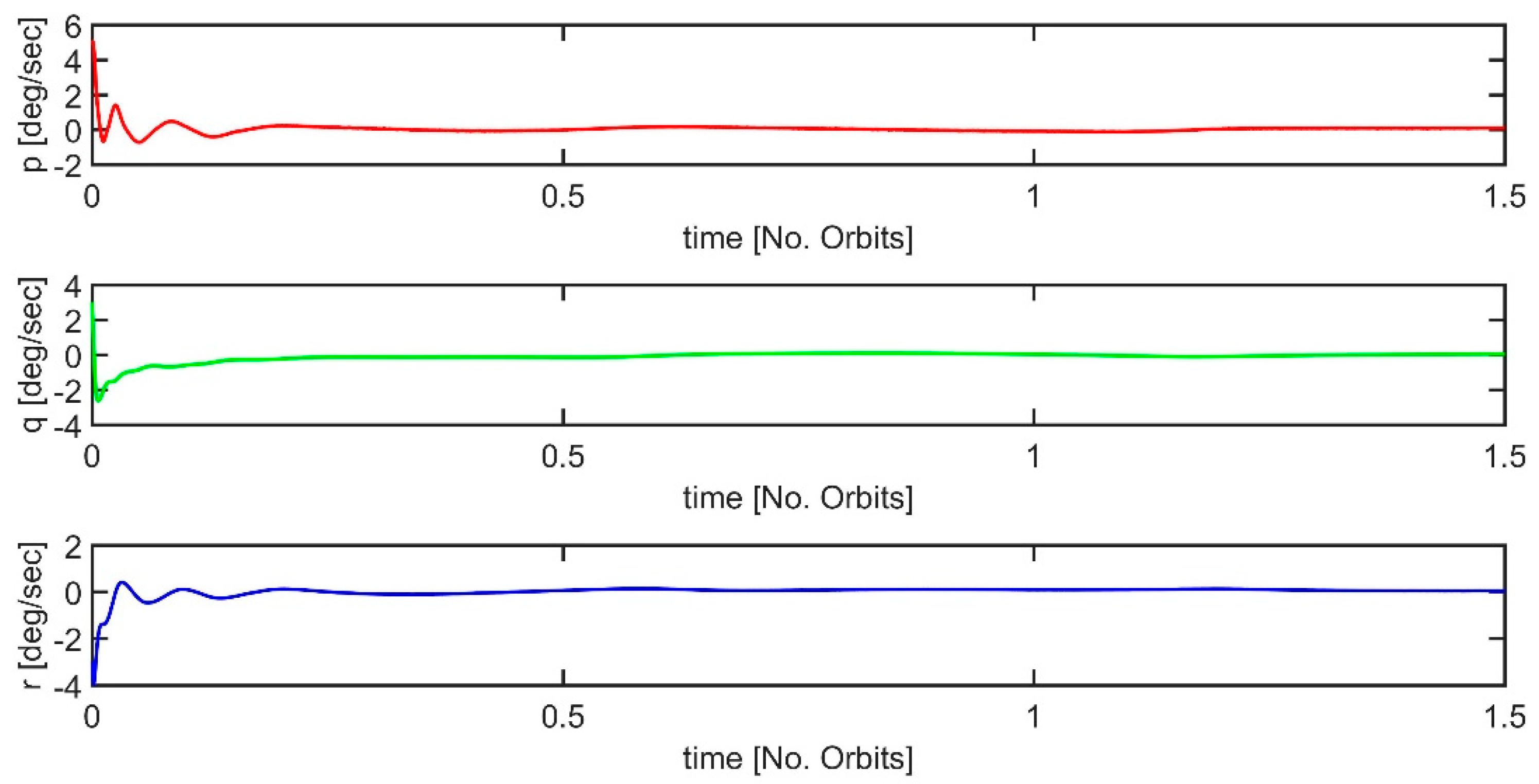
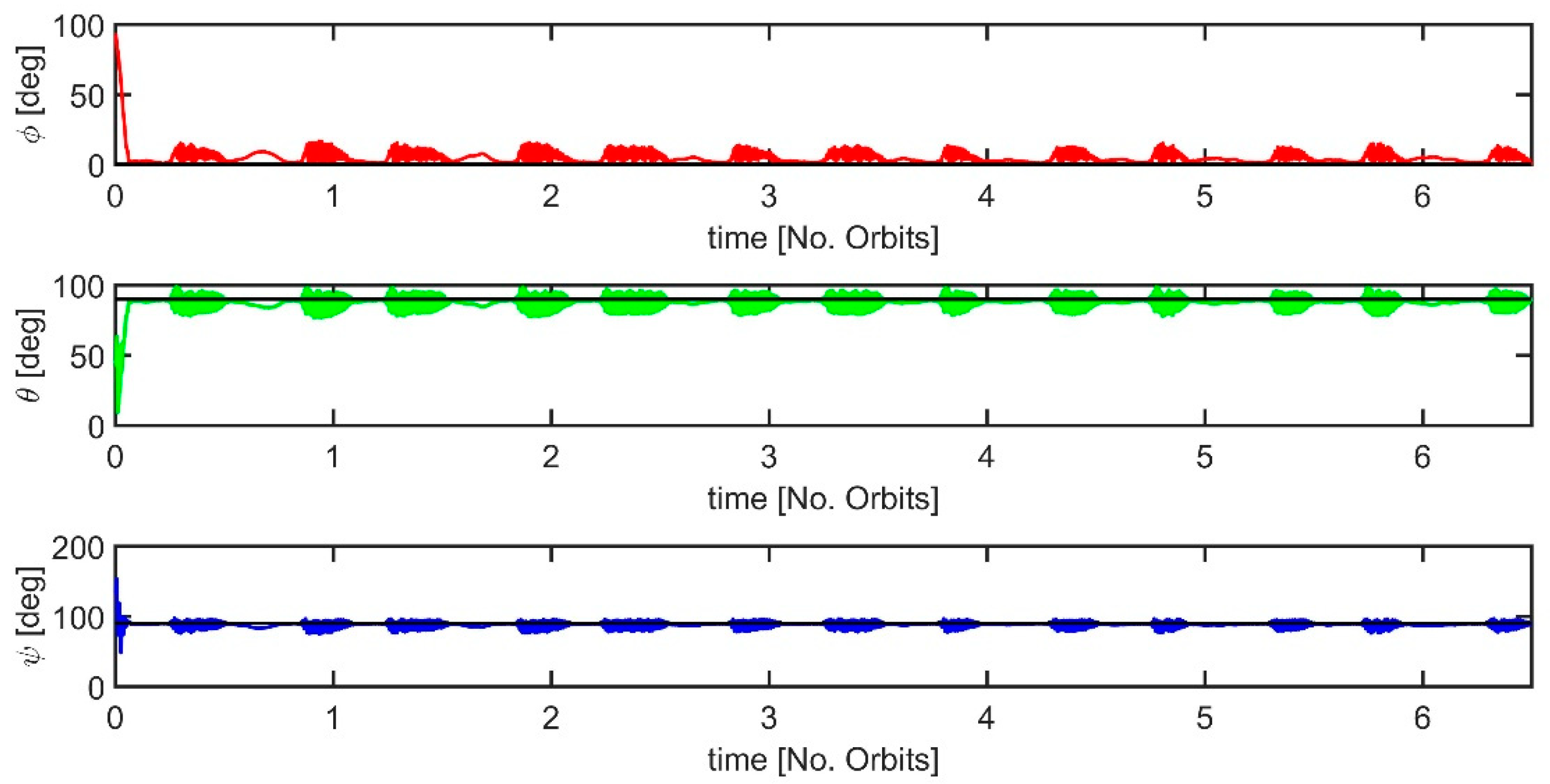
  • the system can produce effective detumbling and stabilization during the pointing phase;
  • the pointing accuracy of the system, though coarse, is acceptable for a backup mode of operations, and considering the lack of attitude information or sophisticate filtering methods (i.e., Extended Kalman Filter);
  • the achievement of some target attitude r ^ can be more challenging, or equivalently less accurate, this is in particular the case for r ^ = [ 1   0   0 ] ;
  • the system is robust with respect to the noise of the calibrated magnetometer (±1 × 10⁻⁶ T) and the perturbation induced by residual dipole moment, gravity gradient and aerodynamic torques.

6. Conclusions

The implementation of a control strategy based on the only measurements data from a MEMS three-axis magnetometer was presented. The strategy allows detumbling and pointing with respect to the geomagnetic field vector, it is tailored for CubeSat applications, requires limited power and is meant to be used as a backup solution, in case of failure of the attitude determination device.
Hardware-in-the-loop simulations are performed to validate the strategy and its implementation on a real CubeSat OBC and a flight proven three-axis magnetometer. The satellite attitude dynamics is simulated, including the perturbation effects of the residual dipole moment, gravity gradient, and aerodynamic torques.
Experimental testing showed that the three-axis detumbling allows reducing the angular rates below 0.1 deg/sec, while the pointing strategy allows achieving the target attitude with an error below 20 deg. In particular, the pointing error increases significantly in the proximity of the magnetic poles, due to the rapid change in the direction of the geomagnetic field vector. This result indicates that the design of a pointing control mitigating this effect would be worth the implementation, and this will be a field of research for the near future.
Further applications of the Hardware-in-the-loop setup are envisioned for the development of the ADCS system designed for the 3U Astro Bio CubeSat (ABCS) and the 6P PocketQube Space Travelling Egg Controlled Catadioptric Object (STECCO) currently developed at the School of Aerospace Engineering. These will include the implementation of a spherical air bearing to simulate microgravity attitude motion of the satellite and testing of magnetometer-only attitude control algorithms.

Author Contributions

Conceptualization and methodology, M.S.F., S.C., A.N., and P.T.; software, M.S.F.; validation, M.S.F. and S.C.; formal analysis, S.C.; investigation, M.S.F. and S.C.; data curation, M.S.F. and S.C.; writing—original draft preparation, S.C.; writing—review and editing, M.S.F., A.N., and P.T.; supervision, A.N. and P.T.; project administration, P.T.”

Funding

This research received no external funding.

Conflicts of Interest

The authors declare no conflict of interest.

References

  1. Swantwout, M. The First One Hundred CubeSats: A Statistical Look. J. Small Satel. 2013, 2, 213–233. [Google Scholar]
  2. Wenschel, L.; Brown, J.; Toorian, A.; Coelbo, R.; Puig-Suari, J.; Twiggs, R. CubeSat Development in Education and into Industry. In Proceedings of the AIAA Space 2006 Conference, San Jose, CA, USA, 19 September 2006. [Google Scholar]
  3. Langer, M.; Bouwmeester, J. Reliability of CubeSats–Statistical Data, Developers’ Beliefs and the Way Forward. In Proceedings of the AIAA/USU Conference on Small Satellites, SSC16-X-2, Logan, UT, USA, 6–11 August 2016. [Google Scholar]
  4. Shou, H.-N. Microsatellite Attitude Determination and Control Subsystem Design and Implementation: Software-in-the-Loop Approach. In Proceedings of the 2014 International Symposium on Computer, Consumer and Control, Taichung, Taiwan, 10–12 June 2014. [Google Scholar]
  5. Stesina, F.; Corpino, S.; Feruglio, L. An In-The-Loop Simulator for the Verification of Small Space Platforms. Int. Rev. Aerosp. Eng. 2017, 10, 50–60. [Google Scholar] [CrossRef]
  6. Wegner, S.; Majd, E.; Taylor, L.; Thomas, R.; Egziabher, D.G. Methodology for Software-in-the-Loop Testing of Low-Cost Attitude Determination Systems, SSC17-WK-09. Available online: https://digitalcommons.usu.edu/smallsat/2017/all2017/5/ (accessed on 30 November 2019).
  7. Klesh, A.; Seagraves, S.; Bennet, M.; Boone, D.; Cutler, J.; Bahcivan, H. Dynamically driven Helmholtz cage for experimental magnetic attitude determination. Adv. Astronaut. Sci. 2010, 135, 147–160. [Google Scholar]
  8. Quadrino, M.K.S. Testing the Attitude Determination and Control of a CubeSat with Hardware-in-the-Loop. Master’s Thesis, Department of Aeronautics and Astronautics, Massachusetts Institute of Technology, Cambridge, MA, USA, 2014. [Google Scholar]
  9. Poppenk, F.M.; Amini, R.; Brouwer, G.F. Design and application of Helmholtz cage for testing nano-satellites. In Proceedings of the 6th International Symposium on Environmental Testing for Space Programmes, ESA Communication Production Office, Noordwijk, The Netherlands, 12–14 June 2007. [Google Scholar]
  10. Delabie, T.; Vandoren, B.; De Munter, W.; Raskin, G.; Vandenbussche, B.; Vandepitte, D. Testing and calibrating an advanced cubesat attitude determination and control system. In Proceedings of the Volume 10698, Space Telescopes and Instrumentation 2018: Optical, Infrared, and Millimeter Wave, SPIE Astronomical Telescopes and Instrumentation, Austin, TX, USA, 10–15 June 2018. [Google Scholar]
  11. Gavrilovich, I.; Krut, S.; Gouttefarde, M.; Pierrot, F.; Dusseau, L. Test Bench for Nanosatellite Attitude Determination and Control System Ground Tests. In Proceedings of the 4S Symposium, Small Satellites Systems and Services 2014, Petro, Spain, 4–8 June 2014. [Google Scholar]
  12. Schwartz, J.L.; Peck, M.A.; Halt, C.D. Historical Review of Air-Bearing Spacecraft Simulators. J. Guid. Control Dyn. 2003, 26, 513–522. [Google Scholar] [CrossRef] [Green Version]
  13. Chesi, S.; Perez, O.; Romano, M. A Dynamic, Hardware-in-the-Loop, Three-Axis Simulator of Spacecraft Attitude Maneuvering with Nanosatellite Dimensions. J. Small Satell. 2015, 4, 315–328. [Google Scholar]
  14. Kuyyakanont, A.; Kuntanapreeda, S.; Fuengwarodsakul, H. On verifying magnetic dipole moment of a magnetic torquer by experiments. In Proceedings of the IOP Conference Series: Materials Science and Engineering, Krasnoyarsk, Russia, 8 November 2018; Volume 297. [Google Scholar]
  15. Lee, D.Y.; Park, H.; Romano, M.; Cutler, J. Development and Experimental Validation of a Multi-Algorithmic Hybrid Attitude Determination and Control System for a Small Satellite. Aerosp. Sci. Technol. 2018, 78, 494–509. [Google Scholar] [CrossRef]
  16. Ousaloo, H.S.; Nodeh, M.T.; Mehrabian, R. Verification of Spin Magnetic Attitude Control System using air-bearing-based attitude control simulator. Acta Astronaut. 2016, 126, 546–553. [Google Scholar] [CrossRef]
  17. Sternberg, D.C.; Pong, C.; Filipe, N.; Mohan, S.; Johnson, S.; Wilson, L.J. Jet Propulsion Laboratory Small Satellite Dynamics Testbed Simulation: On-Orbit Performance Model Validation. J. Spacecr. Rocket. 2018, 55, 322–334. [Google Scholar] [CrossRef]
  18. Tapsawat, W.; Sangpet, T.; Kuntanapreeda, S. Development of a hardware-in-loop attitude control simulator for a CubeSat satellite. In Proceedings of the IOP Conference Series: Materials Science and Engineering, Krasnoyarsk, Krasnoyarsk, Russia, 8 November 2018; Volume 297. [Google Scholar]
  19. Nascetti, A.; Pancorbo-D’Ammando, D.; Truglio, M. Abacus advanced board for active control of university satellites. In Proceedings of the 2nd IAA Conference on University Satellite Missions and Cubesat Workshop, International Academy of Astronautics, Roma, Italy, 3–9 February 2013. [Google Scholar]
  20. Wertz, J.R. (Ed.) Spacecraft Attitude Determination and Control, 3rd ed.; Kluwer Academic Publisher: Dordrecht, The Netherlands, 1978. [Google Scholar]
  21. de Ruiter, A.H.; Damaren, C.; Forbes, J.R. Spacecraft Dynamics and Control: An Introduction, 1st ed.; John Wiley & Sons. Ltd.: Chichester, UK, 2013. [Google Scholar]
  22. Teofilatto, P.; Testani, P.; Celani, F.; Nascetti, A.; Truglio, M. A nadir-pointing magnetic attitude control system for TigriSat nanosatellite. In Proceedings of the International Astronautical Congress 2013, Beijing, China, 23–27 September 2013; Volume 6, pp. 4818–4829. [Google Scholar]
  23. Natanson, G.A.; McLaughlin, S.F.; Nicklas, R.C. A method of determining attitude from magnetometer data only. In Proceedings of the NASA Goddard Space Flight Center, Flight Mechanics/Estimation Theory Symposium, Silver Spring, MD, USA, 1 December 1990; pp. 359–380. [Google Scholar]
  24. Natanson, G.A.; Challa, J.; Deutschmann, J.; Baker, D.F. Magnetometer only attitude and rate determination for a gyro-less spacecraft. In Proceedings of the Third International Symposium on Space Mission Operations and Ground Data Systems, Greenbelt, MD, USA, 1 November 1994; pp. 791–798. [Google Scholar]
  25. Ma, H.; Xu, S. Magnetomter-only attitude and angular velocity filtering estimation for attitude changing spacecraft. Acta Astronaut. 2014, 102, 89–102. [Google Scholar] [CrossRef]
  26. Psiaki, M.L. Global Magnetomter-Based Spacecraft Attitude and Rate Estimation. J. Guid. Control Dyn. 2004, 27, 240–250. [Google Scholar] [CrossRef]
  27. Hart, C. Satellite Attitude Determination Using Magnetometer Data Only. In Proceedings of the AIAA Aerospace Science Meeting Including the New Horizons Forum and Aerospace Exposition, Orlando, FL, USA, 5–9 January 2009. [Google Scholar]
  28. Sugimura, N.; Kuwahara, T.; Yoshida, K. Attitude Determination and Control System for Nadir Pointing Using Magnetorquer and Magnetometer. In Proceedings of the 2016 IEEE Aerospace Conference, Big Sky, MT, USA, 5–12 March 2016. [Google Scholar]
  29. Ma, G.F.; Jiang, X.Y. Unscented Kalman filter for spacecraft attitude estimation and calibration using magnetometer measurements. In Proceedings of the 2005 International Conference on Machine Learning and Cybernetics, Guangzhou, China, 18–21 August 2015. [Google Scholar]
  30. Searcy, J.D.; Pernicka, H.J. Magnetometer-Only Attitude Determination Using Novel Two-Step Kalman Filter Approach. J. Guid. Control Dyn. 2012, 35, 1639–1701. [Google Scholar] [CrossRef]
  31. Carletta, S.; Teofilatto, P. Design and Numerical Validation of an Algorithm for the Detumbling and Angular Rate Determination of a CubeSat Using Only Three-Axis Magnetometer Data. Int. J. Aerosp. Eng. 2018. [Google Scholar] [CrossRef]
  32. Lassakeur, A.; Underwood, C.; Taylor, B. Enhanced Attitude Stability and Control for CubeSats by Real-Time On-Orbit Determination of Their Dynamic Magnetic Moment. In Proceedings of the 69th International Astronautical Congress, Bremen, Germany, 1–5 October 2018. [Google Scholar]
  33. Springmann, J.C.; Cutler, J.W. Magnetic Sensor Calibration and Residual Dipole Characterization for Application to Nanosatellites. In Proceedings of the AIAA/AAS Astrodynamics Specialist Conference, Toronto, OT, Canada, 2–5 August 2010. AIAA-20110-7518. [Google Scholar]
  34. Armstrong, J.; Casey, C.; Creamer, G.; Dutchover, G. Pointing Control for Low Altitude Triple CubeSat Space Darts. In Proceedings of the 23rd Annual AIAA/USU Conference on Small Satellites, Logan, UT, USA, 10–13 August 2009. [Google Scholar]
  35. NASA SP-8058, Spacecraft Aerodynamic Torques; NASA: Washington, DC, USA, January 1971.
  36. Picone, J.M.; Hedin, A.E.; Drob, D.P.; Aikin, A.C. NRLMSISE-00 empirical model of the atmosphere: Statistical comparisons and scientific issues. J. Geophys. Res. Space Phys. 2002, 107, A12. [Google Scholar] [CrossRef]
  37. Reynerson, C. Aerodynamic Disturbance Force and Torque Estimation for Spacecraft and Simple Shapes Using Finite Plate Elements—Part I: Drag Coefficient. Adv. Spacecr. Technol. 2011, 128. [Google Scholar] [CrossRef] [Green Version]
  38. Thébault, E.; Finlay, C.C.; Beggan, C.D.; Alken, P.; Aubert, J.; Barrois, O.; Bertrand, F.; Bondar, T.; Boness, A.; Brocco, L.; et al. International Geomagnetic Reference Field: The 12th generation. EarthPlanets Space 2015, 67. [Google Scholar] [CrossRef]
Figure 1. Sketches of the GeoCentric Inertial frame (GCI) and body-fixed reference frames.
Aerospace 06 00133 g001
Figure 2. Sketch of the magnetometer and magnetorquers position in the body-fixed reference frame.
Aerospace 06 00133 g002
Figure 3. Helmholtz cage at SIA flight mechanics laboratory.
Aerospace 06 00133 g003
Figure 4. Control system for the Helmholtz cage at SIA flight mechanics laboratory.
Aerospace 06 00133 g004
Figure 5. Comparison between measurement by the magnetometer before (red) and after (blue) the calibration.
Aerospace 06 00133 g005
Figure 6. Block diagram of the Hardware-in-the-loop (HiL) setup.
Aerospace 06 00133 g006
Figure 7. Angular rates for the Test Case 1.
Aerospace 06 00133 g007
Figure 8. Euler angles for the Test Case 2, r ^ = [ 1   0   0 ] .
Aerospace 06 00133 g008
Figure 9. Euler angles for the Test Case 3, r ^ = [ 0   0.5 2   0.5 2 ] .
Aerospace 06 00133 g009
Figure 10. Angular rates for the Test Case 2, r ^ = [ 1   0   0 ] .
Aerospace 06 00133 g010
Figure 11. Angular rates for the Test Case 3, r ^ = [ 0   0.5 2   0.5 2 ] .
Aerospace 06 00133 g011
Table 1. Orbital parameters and satellite inertial properties for HiL simulations.
Orbital ParametersAerodynamic Properties
h [km]600CD2.2
i [deg]97.79lx [m]1 × 101
e0ly [m]3.3 × 101
Ω [deg]45lz [m]3.3 × 101
Inertial PropertiesResidual Dipole Moment
m [kg]4 | m m | [Am2]0.1
Jx [kgm2]6.5 × 10³ m m , x [Am2]9.13 × 10²
Jy [kgm2]4.09 × 10² m m , y [Am2]6.32 × 10²
Jz [kgm2]4.09 × 10² m m , z [Am2]9.80 × 10³
Geometric PropertiesMagnetorquers Properties
Ax [m2]1 × 10⁻² N400
Ay [m2]3.3 × 10² A [m2]9.03 × 10³
Az [m2]3.3 × 10² Imax [A]8.3 × 10³
Table 2. Simulation parameters for the three Test Cases (TC).
ParameterTC1TC2TC3
φ, θ, ψ [deg]0, 0, 0175.3, −1.4, 51.7175.3, −1.4, 51.7
ω [deg/sec][5 3 −3][8.5 4.1 4.2]/100[8.5 4.1 4.2]/100
Kd1000300500
Kp02530
r ^     [ 1   0   0 ] [ 0   0.5 2    0.5 2 ]
Table 3. Pointing error Test Cases (TC).
ErrorTC2TC3
Δ φ m i n   [ deg ] 0.02−3.25
Δ φ m a x   [ deg ] 16.670.15
Δ φ m e a n   [ deg ] 4.76−1.95
Δ θ m i n   [ deg ] −13.26−7.68
Δ θ m a x   [ deg ] 8.928.07
Δ θ m e a n   [ deg ] −2.030.02
Δ ψ m i n   [ deg ] −15.73−8.06
Δ ψ m a x   [ deg ] 7.287.68
Δ ψ m e a n   [ deg ] −2.290.01

