Article

Assessment of a Turbo-Electric Aircraft Configuration with Aft-Propulsion Using Boundary Layer Ingestion

by
Rainer Schnell
1,*,†,
Xin Zhao
2,†,
Efthymios Rallis
3,†,
Mavroudis Kavvalos
2,†,
Smruti Sahoo
2,†,
Markus Schnoes
1,† and
Konstantinos Kyprianidis
2,†
1
Institute of Propulsion Technology, German Aerospace Center (DLR), 51145 Cologne, Germany
2
Future Energy Center, School of Business, Society and Engineering, Mälardalen University, SE72219 Västerås, Sweden
3
Department of Mechanincal Engineering, Aristotle University of Thessaloniki, GR54124 Thessaloniki, Greece
*
Author to whom correspondence should be addressed.
These authors contributed equally to this work.
Aerospace 2019, 6(12), 134; https://doi.org/10.3390/aerospace6120134
Submission received: 8 November 2019 / Revised: 9 December 2019 / Accepted: 11 December 2019 / Published: 16 December 2019
(This article belongs to the Special Issue Progress in Jet Engine Technology)

Abstract

:
In this paper, a turbo-electric propulsion system was analyzed, and its performance was assessed. The aircraft considered here was a single-aisle, medium-range configuration targeting a capacity of 150 Pax. The propulsion concept comprised two boosted geared turbofan engines mounted under-wing. Those main engines were supported by an electrically driven aft-propulsor contributing to the thrust generation and by taking advantage of ingesting the boundary layer of the fuselage for potentially higher levels of propulsive efficiency and allowing for the improved operation of the main engines. The performance assessment as carried out in the context of this paper involved different levels: Firstly, based on the reference aircraft and the detailed description of its major components, the engine performance model for both main engines, as well as for the electrically driven aft-propulsor was set up. The methodology, as introduced, has already been applied in the context of hybrid-electric propulsion and allowed for the aforementioned aircraft sizing, as well as the subsequent gas turbine multi-point synthesis (simulation). A geared turbofan architecture with 2035 technology assumptions was considered for the main engine configuration. The present trade study focused on the design and performance analysis of the aft-propulsor and how it affected the performance of the main engines, due to the electric power generation. In order to allow for a more accurate description of the performance of this particular module, the enhanced streamline curvature method with an underlying and pre-optimized profile database was used to design a propulsor tailored to meet the requirements of the aft propulsor as derived from the cycle synthesis and overall aircraft specification; existing design expertise for novel and highly integrated propulsors could be taken advantage of herein. The resulting performance characteristics from the streamline curvature method were then fed back to the engine performance model in a closely coupled approach in order to have a more accurate description of the module behavior. This direct coupling allowed for enhanced sensitivity studies, monitoring different top-level parameters, such as the thrust/power split between the main engines and the aft propulsor. As a result, different propulsor specifications and fan designs with optimal performance characteristics were achieved, which in return affected the performance of all subsystems considered.

Graphical Abstract

1. Introduction

Facing an exponential growth in civil air traffic over the next decades [1], accompanied with growing skepticism in the population towards air traffic in general, almost all major economies in the world initiated dedicated research efforts to compensate for or, at least, minimize the negative impacts induced by aircraft emissions. In Europe, the initial targets, formulated in the context of ACARE’s visions 2020 in the early 2000’s within an alliance of research organizations, universities and industry, were continued and extended, resulting in an updated version of its Strategic Research Agenda named Flightpath 2050 [2]. The major targets laid out therein concern a significant reduction in CO2, NOx and noise emission; those ambitious goals are expected to be reached with major contributions from engine and aircraft technology, as well as air traffic management (ATM) and operations in general. Continuous and rather evolutionary development of gas turbine technology already led to a major reduction in specific fuel consumption (SFC) for the latest generation of A320 equipped with new engine technology (NEO) compared to 2000’s technology. This trend of improving conventional technology at module and system level is expected to continue, but also novel and more revolutionary concepts are to be considered, due to the already very high level of maturity of the existing technology. In this context, complementing the classical gas turbine cycle with electrical components is expected to open the design space further, and hence, offering more potential to increase overall performance. Whereas, purely electrical driven aircraft does not seem a viable option mid-term, due to excessive energy density requirements, well exceeding the technically achievable limits (at least at a larger scale), turbo- and hybrid-electric configurations may have potential benefits and are subject to a growing number of research activities worldwide and within Europe. Most of those concepts have in common that a gas turbine is being used for providing the major portion of the energy, whereas, a combination of power extraction from the main engine and power input from batteries is also considered in various arrangements. The potential advantages of such configurations at a system level can be summarized as follows:
  • Improved operability of the gas generator (e.g., by minimizing cooling requirements or enhancing component performance in terms of stall margins, resulting in reduced required variability),
  • possible re-(down-)sizing and optimization of the gas generator (e.g., by relieving the core engine requirements by additional power input from an electrical source at the most demanding, and hence, sizing relevant mission points), and
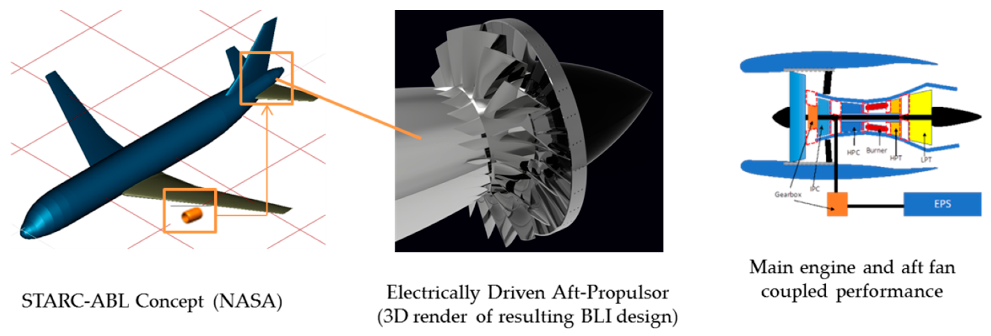
  • decouple the location of thrust induction from power generation and thereby further opening the entire design space and allowing for novel aircraft configurations with improved engine integration (e.g., by ingesting the fuselage boundary layer).
The first two points have been addressed in several studies, and their potential benefits were quantified, e.g., in References [3,4,5,6]. The third point entails a large variety of possible configurations and arrangements, of which one was selected and is subject to the present study: The chosen configuration comprises a conventional tube-and-wing aircraft with two main under-wing engines producing the major portion of the required thrust. An additional, electrically driven propulsor is introduced in the backend of the aircraft fuselage and contributes to fulfilling the overall thrust requirements. Due to this arrangement, the aft-propulsor is able to ingest the fuselage boundary layer, and hence, may operate at higher levels of propulsive efficiency; this is expected to increase the overall efficiency of the entire propulsion system, potentially translating into an SFC benefit. However, the additional weight and drag introduced by both, propulsor and electrical system, along with necessary modifications of the aircraft (e.g., due to a possible re-design of the entire empennage) will compromise the potential benefits, which makes the evaluation of the given technology at the system level a necessary step. In general, this arrangement is considered to be the most conservative among more radical and future headed scenarios since it retains most of the classical tube-and-wing layout, including the benefit of existing gas turbine technology.
The potential advantages of a boundary layer propulsion system were identified and addressed already in the mid 40’s of the last century [7], and configurations taking advantage of this effect have been broadly investigated ever since. The most comprehensive overviews and framework of equations, more or less universally applicable at a conceptual level to any new aircraft (A/C) configuration, can be found in Reference [8], and a more recent one in the direct context of novel aircraft configuration in Reference [9]. The configuration, as studied in the context of this paper, has also been introduced and studied by other researchers, one of the most comprehensive and prominent one being provided by NASA named Single-aisle Turboelectric Aircraft with an Aft Boundary Layer (STARC-ABL) in Reference [10]. More recent studies of this particular configuration are not only presenting a refined overall performance assessment at higher levels of fidelity [11,12], but furthermore addressing specific aspects, such as the Computational Fluid Dynamics (CFD)-based design optimization of the aft propulsors’ intake [13]. Those investigations are complemented by other studies of similar concepts, however, in most cases at a lower level of fidelity and more conceptual in nature [14,15]; all studies, however, suggest a benefit in terms of mission-based block fuel and encourage a number of activities dedicated to this particular concept. Based on the available data and modelling approaches as described in the given literature (or a lack thereof), the main research questions that will be addressed in the present article shall be derived and posed at the next chapter.

2. Research Objectives and Layout of the Present Study

In light of the anticipated technological advances outlined above, the main mechanisms defining the system performance of the given configuration are the following:
  • The amount of boundary layer captured by the aft-propulsor and hence, the level of achievable propulsive efficiency;
  • The performance and design of the aft-fan;
  • The performance of the main engine and its components, in particular considering that power is being extracted and transferred to drive the aft propulsor;
  • The performance and weight of the electrical system.
All mentioned aspects are inherently inter-dependent in such way that, e.g., the amount of captured boundary layer is influenced by the aft-propulsor dimensions, which are driven by its pressure ratio (FPR) and mass flow rate, resulting from the level of power input to the aft-fan as being extracted from the main engines; this, in return, drives the performance of the gas turbine. One of the main design choices at top-level to be made is the thrust or power split between the main engine(s) and the aft propulsor. At the module level, FPR then has to be chosen to initiate more detailed design considerations of the aft-fan. A detailed knowledge of the boundary layer (or respective momentum deficit) that can be ingested into the aft-fan typically requires a dedicated and CFD based design effort of the fuselage and the intake; some further information can be found in References [10]. Since the present study was carried out exclusively at the conceptual level, the introduction of CFD was not considered. A sensitivity analysis conducted for the inlet momentum deficit, as potentially being captured by the aft-fan; several design efforts were realized at different levels of momentum deficit for a given set of power extraction and FPR. This was used to explore the design space, and served as a guide to choose the top-level cycle and fan parameters, allowing for a more detailed design of the fan afterwards. An underlying performance model of the gas turbine was used to evaluate the performance of the cycle, taking advantage of multi-point synthesis matching theme at key mission points. In this context, the main questions that will be subsequently addressed and answered in the following chapters, also defining the layout of the present study, are the following:
(1)
What is the sensitivity of the system top-level parameters, here mainly being the power extraction from the main engine low speed shaft (PWX46) to the aft-fan (PWX48), as well as the aft-fan FPR, on the overall performance metrics (downselection)?
(2)
What implications and challenges do those choices impose on the conceptual design of the aft-fan and to what extent do they affect the gas turbine/main engine performance?
Since addressing those questions always has to be seen in the light of the assumptions that were made and the methods being used, the next chapter will summarize both in order to make the results as transparent as possible. Figure 1 highlights the main components of the present study in a schematic manner: The actual aircraft as used in this study, and the underlying mission will be described in Section 3.1. The gas turbine with all its components represented by a thermodynamic cycle model is introduced and assessed in Section 3.2 and the aft-propulsor design, which was realized with a streamline-curvature based design method, will be discussed in Section 3.3; the respective coupling of the cycle model with the streamline curvature method will be described and discussed in Section 3.4. The main results, quantifying the overall potential of the given concept, will then be summarized in Section 4.

3. Assumptions and Methodology

3.1. Aircraft and Mission Profile

An A320-like, single-aisle aircraft, more details of which are given in this paragraph, was the basis of the present study. The thrust requirements of the main mission points are summarized in the following Table 1:
Since the concept clearly aims at fuel burn benefits at Cruise conditions, only the main mission points for the aerodynamic and thermal design of the gas turbine, as well as cruise were included in the sensitivity analysis. No full mission analysis was carried out for boundary layer ingestion (BLI) scenarios, but the resulting block fuel-saving potential was estimated through the use of exchange rates. Those exchange rates translated the change in cruise SFC, weight and drag into a respective change in mission fuel burn; all necessary details regarding this conversion are provided in Section 4.3.3. More information on the mission characteristics and resulting engine performance of the baseline engine at all ratings can be found in Reference [6] and Table A1 in the Appendix A. Regarding the aircraft geometry, the Central Reference Aircraft Data System (CeRAS) model in Common Parametric Aircraft Configuration Schema (CPACS) format was available [16] representing a validated and re-engineered version of an A320. Its main geometric features are summarized in Table 2.
The resulting performance parameters were also available through the Environmental Assessment (EVA) framework to allow for a coupled consideration of aircraft and engine performance for a given mission profile. The specifications of EVA can be found in Reference [17], and more information will be provided in the following chapter when describing the main engine cycle. The tail cone geometry of the given aircraft model was used within this study to define the location where the fuselage diffusion begins and also to define the minimal hub diameter of the aft-fan. One important constraint applied to this study was to fix this radius at r = 0.37 m in order for the tail-cone propulsor to be structurally integrated and comply with the given fuselage geometry (see also [10] in which a similar arrangement and values were used). Regarding the fuselage boundary layer, a rough estimate based on simple turbulent flat plate theory using (1/7th) power law [18] was made, taking into account the given fuselage dimensions and aircraft mission parameters (flight Ma and altitude). Together with aft-propulsor mass flow rate, this profile defined the incoming momentum deficit (see Figure 2), which also was assumed to be axisymmetric. The boundary layer theory applied did not include any pressure gradient, and all the integrated fuselage friction was directly translated into a corresponding average total pressure loss. This treatment of the incoming boundary layer, despite being practically applicable and reasonably representing the prevailing flow physics at conceptual level, is only a first order estimate and the incoming momentum deficit largely depends on the fuselage and intake design, as well as the respective diffusion (and also the real boundary layer height may be substantially smaller or bigger [19]). Hence, the uncertainty in predicting the real achievable incoming momentum deficit was considered in a sensitivity study.

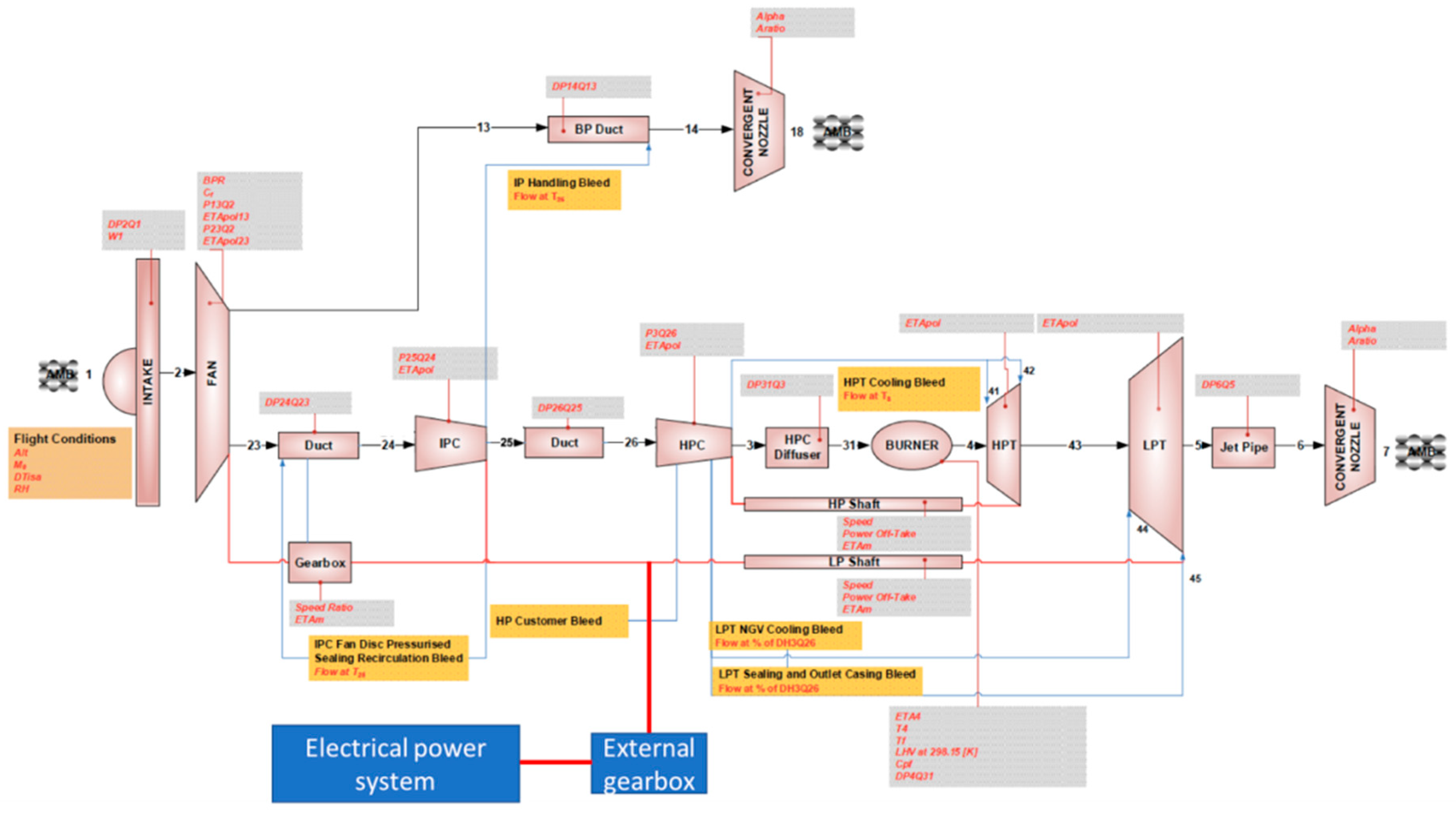
3.2. Main Engine Gas Turbine Cycle

As far as the two under-wing main engines are concerned, a geared turbo-fan architecture was envisioned, and the overall engine performance modelling schematic (with corresponding power extraction from the low-speed shaft) is shown in Figure 3.
Entry into service (EIS) 2035 component polytropic efficiency levels and maximal metal temperatures were being introduced into the performance model. The values for the engine specific thrust (SFN), gas generator overall pressure ratio (OPR), jet velocity ratio VcoldQhot and pressure ratio split exponent (PRn) at Cruise conditions emerged from a performance optimization of this particular engine as described in greater detail in Reference [6]. Those values or respective limitations were fixed in the present study by applying a multi-point cycle synthesis for different and relevant mission points (for the BLI cases the main engine’s fan inlet mass flow w2 was fixed rather than SFN (see Section 4)); here mainly the aerodynamic design point hot-day Top of Climb (TOC) and hot-day Take-Off (TO). This set of parameters and respective matching thereof, more details of which are given in Table A2 in Appendix A, also defined the baseline engine (without power extraction and aft-fan) to which all cases with aft-propulsion and BLI will be assessed against. Originated from the baseline, for all the BLI cases, it is important to highlight that the very same parameters of the gas generator (OPR, PRn, VcoldQhot and T4 at cruise, as well as the turbine maximum metal temperatures) were retained with power extraction and a respective thrust contribution from the aft-propulsor. This resulted in comparable levels of core efficiency and allowed for a better analysis as to what mechanism is responsible for the potential or penalty. As illustrated in the matching scheme Table A2 in Appendix A, for all the engine performance simulations, a multiple point synthesis was applied to keep the aforementioned main engine parameters constant. At multiple synthesis level, Bypass Ratio (BPR) and FPR at TOC were varied for the constant VcoldQhot and T4 at cruise, and compressor pressure ratios at TOC were varied for constant OPR and PRn at cruise. Metal temperatures were fixed through varying the corresponding turbine cooling flow. The minor effect from the selection of the cooling flow extraction point was, however, neglected—hence, the fixed extraction point defined. At a single point level, a constant fan inlet mass at TOC was set, in order to achieve a constant main engine fan size instead of a constant SFN. For a given FPR and BPR from synthesis level, as well as a constant fan inlet mass flow at TOC, T4 at design point hot-day TOC was varied for matching the thrust requirement and the power delivered to the BLI fan. For the BLI fan, shaft power input and the pressure ratio of it were given, and the air mass flow going through it was varied to consume the power fed in. The aforementioned calculations were realized within the computational framework EVA, where disciplines like aircraft sizing and performance, as well as engine performance with multi-point cycle synthesis matching scheme are incorporated [17].

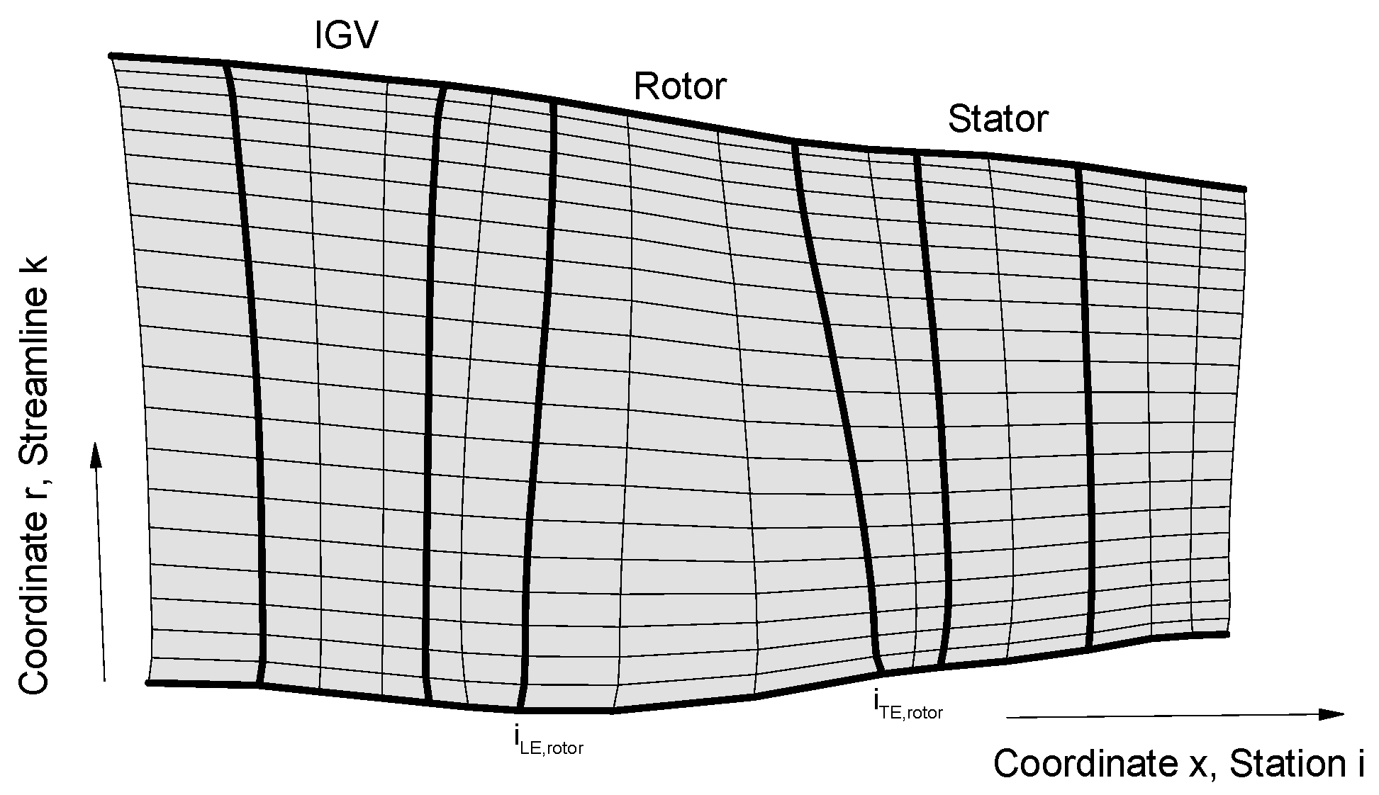
3.3. Propulsor Conceptual Design

The conceptual design of the aft-propulsor was carried out using a streamline-curvature method in a through-flow manner using the DLR’s Advanced Compressor Design Code (ACDC) [20,21]. This study focused on this particular component, due to the more unknown, and to some extent, unconventional design space (as compared with the main engine component). The method requires a computational grid in a through-flow plane—as shown in Figure 4—as an input, with a number of streamlines in the radial direction (k) defined at different axial locations (i). The position of each blade row is given by its respective leading and trailing edge index I; this also fixes the axial chord of each blade row. The grid also defines the annulus lines of the hub (k = 0) and the tip (k = kmax). Other input parameters to be specified are the number of blades for each blade row, the rotors’ rotational speed and the mass flow rate. Together with the physical boundary conditions defining the inlet thermodynamic states and flow kinematics (total pressure and temperature and flow angles, all as a radial profile and stemming from the fuselage boundary layer profile in the case of a BLI assessment), the method provides all necessary data to describe and assess the stage performance in the given through-flow plane (=meridional plane along the machine axis, as shown in Figure 4, also referred to as S2M-plane). Essentially two modes are available: A design mode, which requires an a priori definition of the radial distribution of the rotor total pressure ratio (the average of which is the design target resulting from the engine performance) and outlet guide vane (OGV) exit flow angle (typically chosen to achieve swirl free outflow) at design conditions. The second mode enables the assessment at off-design conditions and the calculation of respective performance characteristics over the entire speed range. Both modes assess the fan design by taking advantage of a large database of pre-optimized profiles (see References [20,21] for more details), together with standard correlations taking into account endwall and tip leakage effects. One of the advantages of the existing database is that it consists of performance parameters, such as profile losses and deviation being directly linked to geometric parameters. Hence, a full 3D geometry of the whole stage is available through interpolation within the database right away and allows for a seamless subsequent assessment and verification of the design using CFD (not being part of the conceptual design and not considered here). The design strategy for the aft propulsor and rationale for the main design decisions will be described in more detail in the corresponding Section 4.2.2. From the aforementioned method description, it is obvious, however, that the number of parameters to be specified requires a fair amount of design expertise and is not straight forward or directly to be taken from textbooks. This underlines the necessity for an inter-disciplinary exchange, involving experts with different backgrounds when exploring entirely new design spaces.

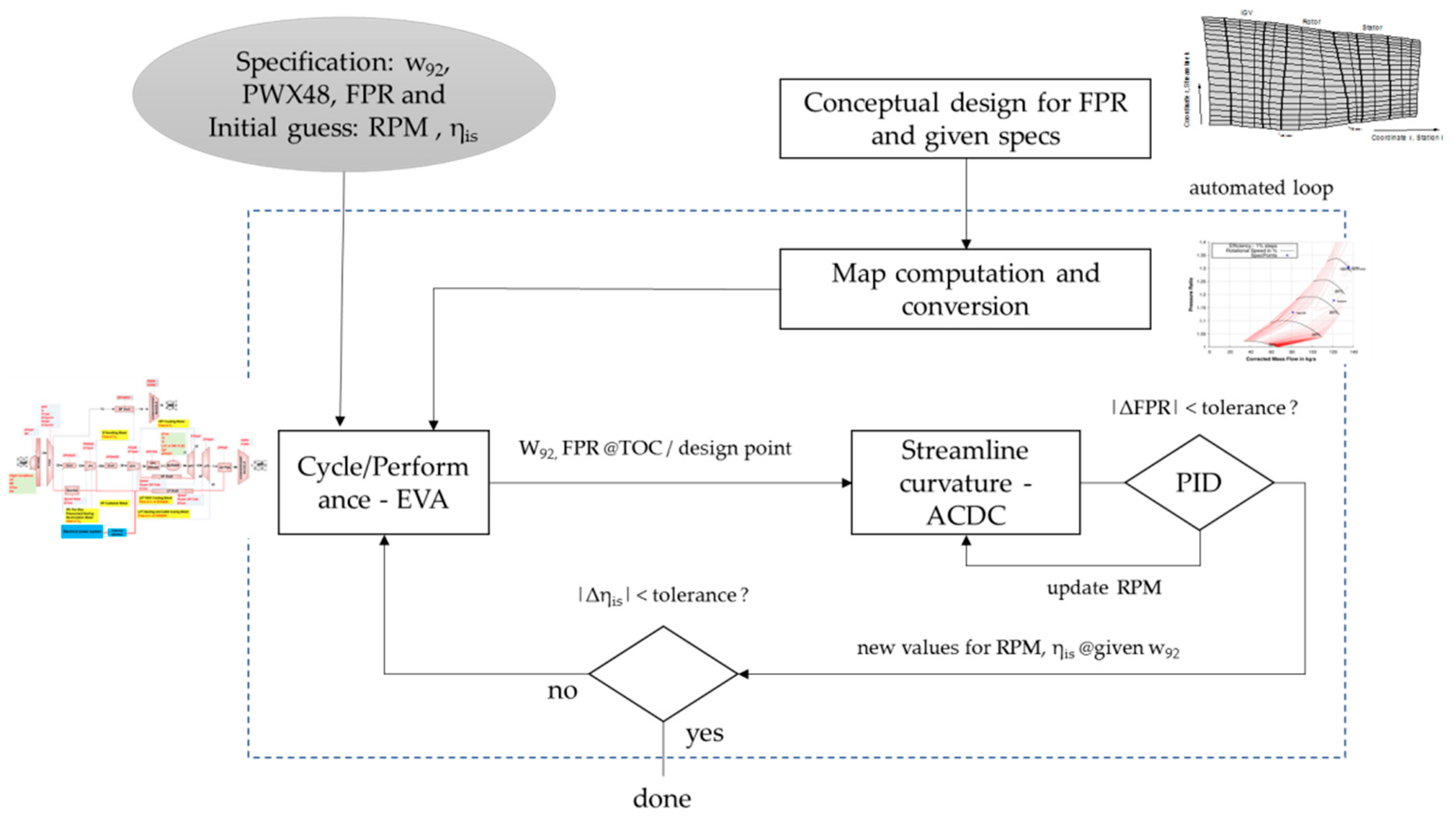
3.4. Method Coupling Procedure and Performance Characteristics Sensitivity

The consistency between module performance and the thermodynamic model at cycle level is of importance in order to gain knowledge of realistically achievable efficiency levels at design conditions under given constraints and in particular to describe the modules’ off-design behavior. The latter one is of particular significance for the mission analysis and also to support early design decisions, such as the necessity for introducing variability, due to a compromised stall margin of the respective component. Typically, there are several ways of describing the performance of the respective module (here aft-fan) at cycle level:
  • Use and scaling of a standard component map (either from open literature or from an internal database, depending on the level of knowledge);
  • The scaling of a more tailored map (e.g., stemming from initial design considerations of the respective module);
  • Direct use of the unscaled map, e.g., from more advanced conceptual design iterations of the module; or
  • A direct coupling between the cycle performance and the component design, typically realized in an iterative manner for each mission point (a zooming-like approach).
The latter approach is visualized in Figure 5: It starts with a given specification in terms of mass flow rate w92, FPR and a first assumption of the component efficiency level at the given mission point. Those data were exchanged with the streamline curvature method, which iterates by changing the rotational speed (RPM) to meet the targeted mass flow rate and FPR using a controller with Proportional, Integral and Differential (PID) characteristics. The efficiency level is a result, and all data were transferred back to the cycle. This procedure is carried out repeatedly until consistency between both models is achieved with a given accuracy. Typically, the method convergences after approximately five outer iterations, with 3–4 inner iterations of the Streamline-Curvature (SLC) based method to adjust the operating conditions. Although some effort was put into realizing this direct coupling procedure, it only seems to have advantages when creating maps being more computationally expensive (e.g., by CFD) than being achieved with a through-flow based approach (which needs less than a minute to produce the entire map).
The advantage (or sometimes necessity) of having more detailed knowledge about the module performance at off-design conditions is highlighted in the next two figures, Figure 6 and Figure 7. In the plots, different performance characteristics of the aft-fan are shown and compared. The obvious difference in their respective shape to a large extend is driven by the difference in FPR on the one hand and different design philosophies (here, choices of rotor tip speed) at given FPR on the other hand. It is presumed, for example, that the standard and pre-existing maps, before being scaled down to match the target FPR, were originally designed for a higher FPR. This design yields an inherently steeper characteristic, due to higher and (supposedly) well supersonic relative rotor tip Mach numbers as compared to subsonic or close to sonic tip Mach numbers at the rotor inflow for the tailored and SLC based designs at lower FPR (1.2). Since at this point, no BLI scenario is considered and all maps were generated with radially constant inlet conditions, the difference in the shape of the maps is solely attributed to different design targets and philosophies. Apart from the performance characteristics, Figure 6 also shows a direct comparison of the location of the considered mission points when using standard maps (Figure 6a) and maps (Figure 6b) stemming from a first conceptual study of the aft-propulsor for a chosen FPR = 1.2. Due to a constant power off-take in all mission points, the Cruise and Top-Of-Climb points almost collapse and, contrary to the main engines’ operation, the descent point is also located at very high RPM, due to the high power input. A fixed nozzle operation was considered for all simulation points, and the nozzle is unchoked at all conditions for given levels of FPR. One of the most important observations concerns the aft-propulsor stall margin at Take-Off conditions. Whereas, the standard maps suggest sufficient reserves in terms of stall margin, due to the much steeper speed lines (representing a more transonic design or even the behavior closer to a multi-stage Low-Pressure Compressor (LPC)), the actual location of the Take-Off point is closer to the expected component’s stability limit. However, this needs to be further quantified (e.g., as shown in Reference [22]), although the Aft-Fan stall margin was not considered explicitly in all design efforts. Moreover, the corresponding rotational speed is substantially different, which is important for designing the electrical system. By comparing the maps from different design rationales or top-level choices in Figure 7, all stemming from a conceptual design using the through-flow approach, one can make a similar observation regarding the stall margin at Take-Off conditions: Due to the steeper characteristic of a low-work coefficient Ψ design, and hence, higher rotor tip speed, the stall margin is inherently greater as compared with a high-Ψ design at given FPR (ore details on the overall design rationale and choice and meaning of the working coefficient are provided in Section 4.2.2). Increasing the FPR, however, seems a more viable option to maintain a necessary stall margin of the aft-fan. It is important to note that the through-flow results do not provide the necessary fidelity to accurately predict the stall margin on an absolute basis, but rather give an indication and trend when comparing the different design strategies (in fact the stall line was estimated by omitting points with a lower than a given average de-Haller number). However, as stated at the beginning of this chapter, early design choices to be made at cycle level regarding a necessary variability can be supported with a better idea of the module’s off-design performance, and hence, additional iterations between the different design teams avoided.

4. Results and Discussion

4.1. Sensitivity Studies

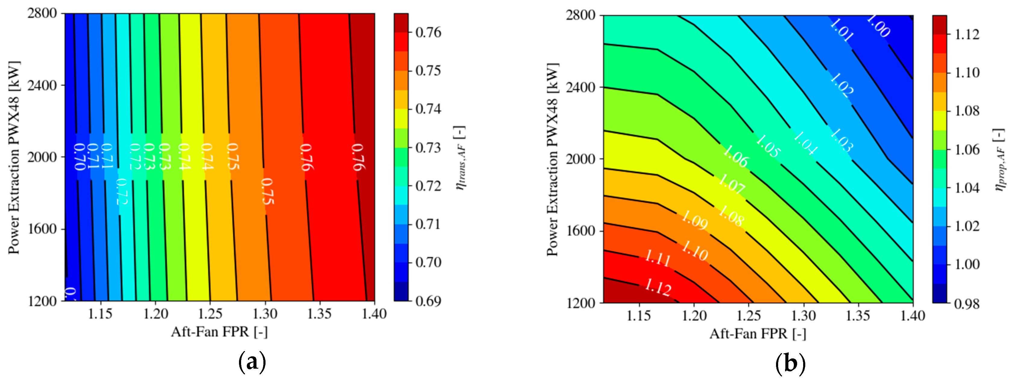
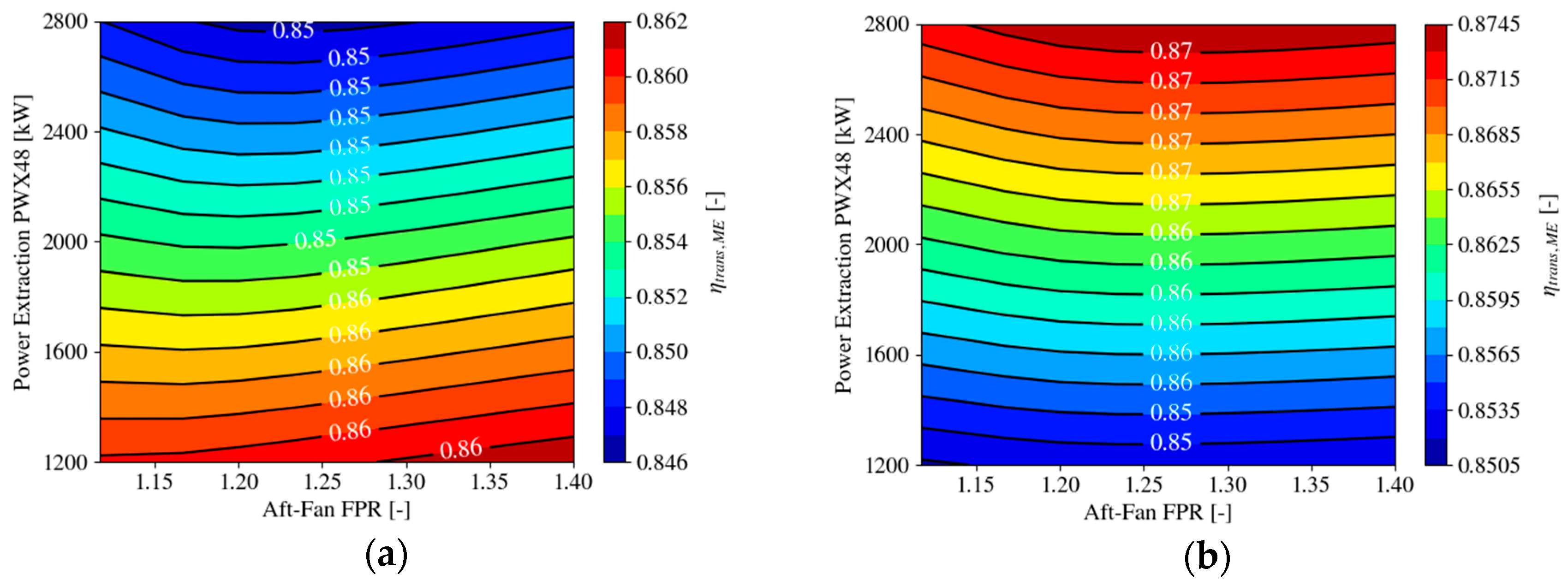
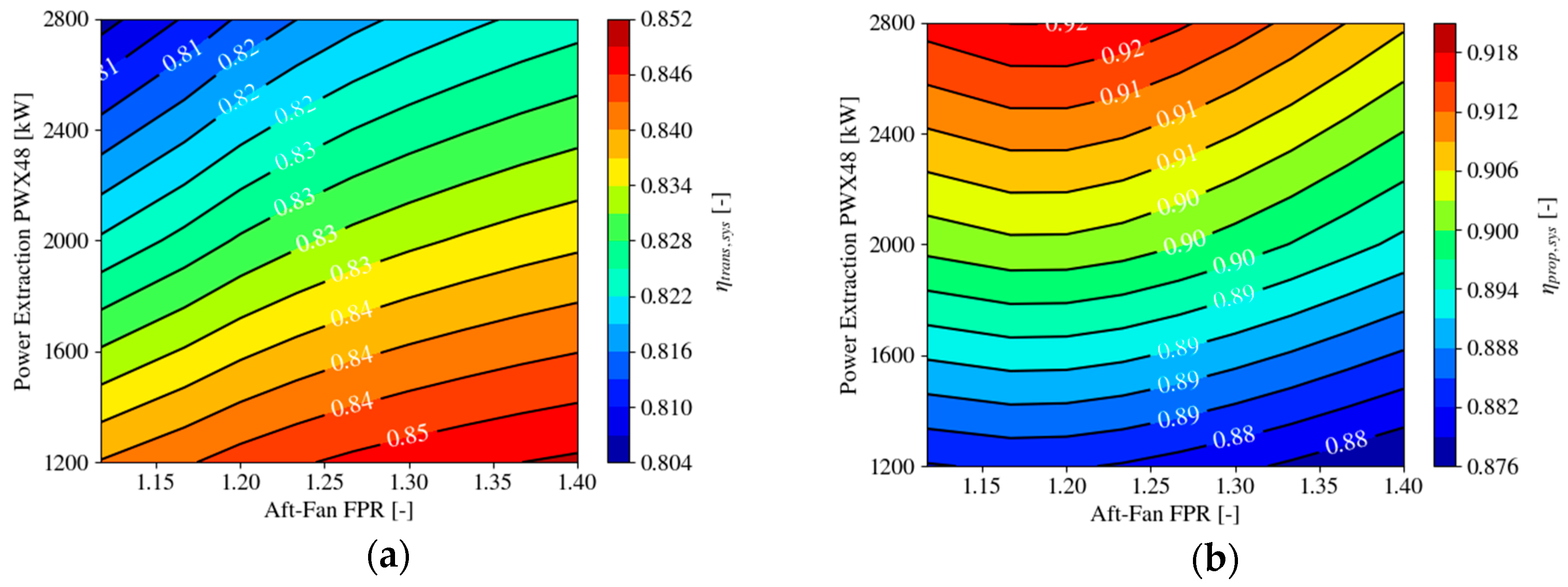
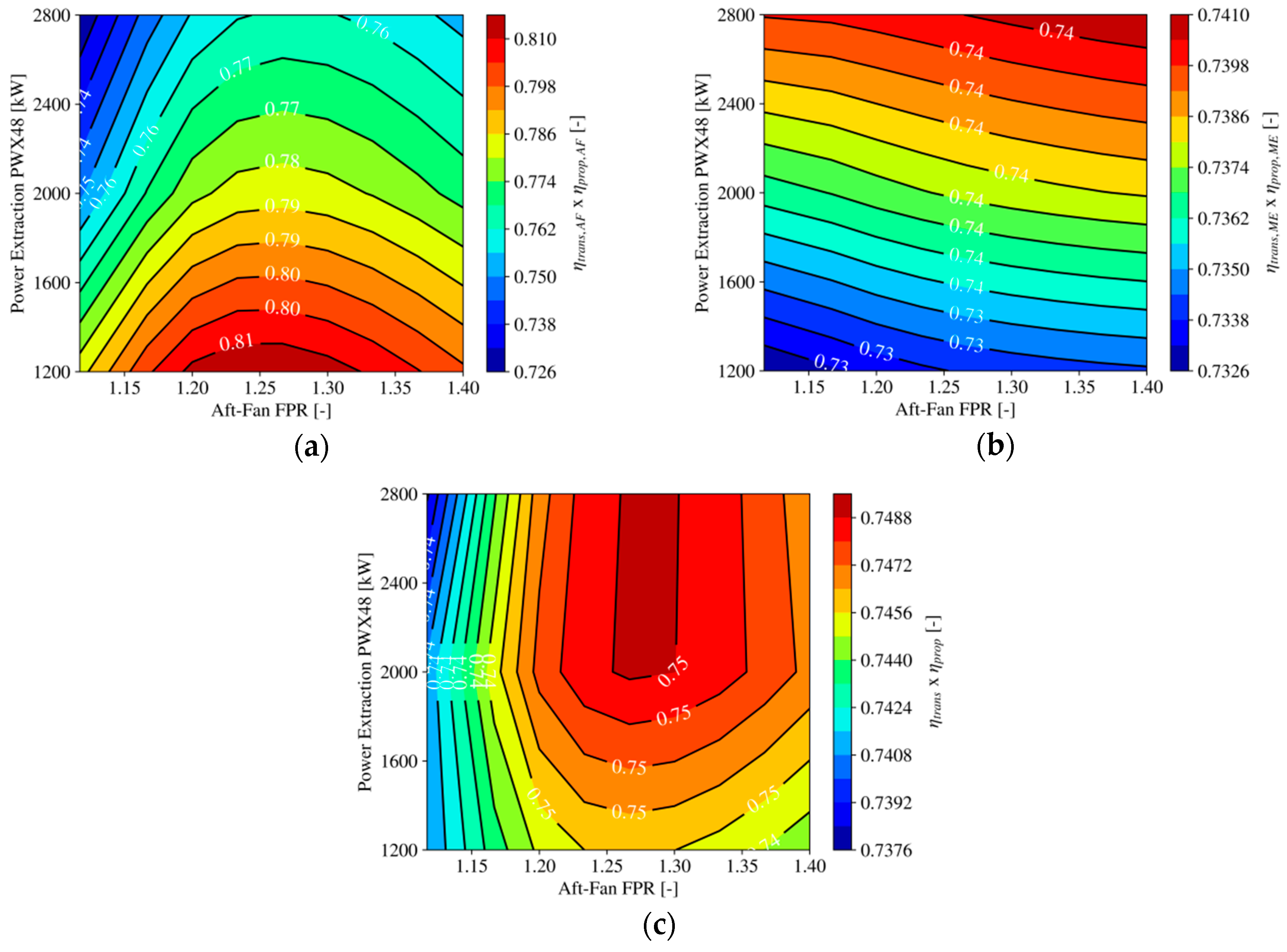
4.1.1. Efficiency Definitions and Figures of Merit

Before discussing the results of the sensitivity analysis in the following sub-chapters, the framework of equations used for the analysis shall be laid out first, considering the assumption made in the previous chapters. This will be done at the thermodynamic level; hence, only average and mixed out states will be regarded with a number of simplifications made for the sake of clarity and the conceptual nature of the entire study. As far as the constant net thrust (FN) at the given mission point is concerned, contributions from the aft-fan (AF) and the two main engines (ME) are included in the total sum as follow:
F N = F N A F + F N M E = c o n s t .
In this way, when the aft-fan produces more thrust, the main engine contribution will be smaller. The main figure of merit that will be focused on in the following chapter is the uninstalled specific fuel consumption S F C u n i n s t a l l e d
S F C u n i n s t a l l e d = v 0 η o v , s y s t e m · F H V .
Technically the term “uninstalled” is somewhat misleading since one major effect of the aft propulsor’s installation into the aircraft, which is the incoming momentum deficit resulting from the fuselage boundary layer, is inherently included in Equation (2) as it will be shown in the next paragraphs. It will be used nonetheless in order to be in line with the wording stemming from classical, under-wing engine integration. It is reasonable as well since non-thermodynamic effects, such as engine weight and drag are not included herein. At given flight speed v 0 , uninstalled SFC is driven by the overall efficiency of the system η o v , s y s t e m consisting of both, the aft-fan and the main engine. This overall efficiency at the system level is a function of core efficiency ( η c o r e ) of the gas generator, transmission efficiency ( η t r a n s ), propulsive efficiency ( η p r o p ), mechanical efficiency ( η m e c h ) (friction in bearings, duct and gearbox losses etc.) and the efficiency of the electrical system ( η e l ):
η o v , s y s t e m = f ( η c o r e , η t r a n s , η p r o p , η m e c h , η e l ) .
The last two, η m e c h and η e l , were included in the performance analysis, but kept at constant values of ηmech = 0.99 and ηel = 0.95, and hence, shall not be considered further on as part of the sensitivity (for more on the efficiency of the electrical system see Section 4.3.1. Following the definitions of both, propulsive and transmission efficiency, it is worthwhile looking at those quantities separately for the aft-fan and the main engine, as well as at a system level, in order to better understand the trades to be made. Starting with the main gas turbine engine, the conventional definitions of the propulsive efficiency η p r o p , transfer efficiency η t r a n s and core efficiency η c o r e are a priori applicable and useful. The core efficiency, which per definition is the ratio of the power available after all the power requirements of the core compression processes (including power off-take) are satisfied, E c o r e , and the power as introduced by the fuel flow, E f u e l ,:
η c o r e = E c o r e E f u e l .
In the same vein, the transmission efficiency η t r a n s , M E is defined as the quality of the power transfer from the core stream to the bypass stream. This translates to the ratio of the change in kinetic energy of the jets in the bypass and core, Δ E k i n , j e t , to the useful power of the core, E c o r e :
η t r a n s , M E = Δ E k i n , j e t E c o r e .
The propulsive efficiency is defined as the useful propulsive power over the change in jet kinetic power:
η p r o p , M E = F N M E v 0 Δ E k i n , j e t .
With the definition of the stations 18 (bypass nozzle throat) and 7 (core nozzle throat), as shown in the gas turbine schematic, and accounting for the power-off take from the main engine core, as well as removing the system kinetic power, due to the flight velocity w 2 v 0 2 , the transmission efficiency of the main engine can be written as:
η t r a n s , M E = 0.5 · ( w 18 v i d , 18 2 + w 7 v i d , 7 2 w 2 v 0 2 ) E p , c o r e w 7 v 0 2 / 2 P W X 46 η L P T
Here E p , c o r e is the core exit potential power, and the core exit is where the fan core and LPC power requirements are satisfied in the low-pressure turbine (LPT) expansion. The core flow energy used for the production of PWX46 through the LPT, as well as the core stream kinetic energy w 7 v 0 2 / 2 , need to be subtracted from the potential power in the main engine in order to define the transmission efficiency. The propulsive efficiency is given by:
η p r o p , M E = F N M E v 0 0.5 · ( w 18 v i d , 18 2 + w 7 v i d , 7 2 w 2 v 0 2 ) = v 0 [ w 18 ( v i d , 18 v 0 ) + w 7 ( v i d , 7 v 0 ) ] 0.5 · ( w 18 v i d , 18 2 + w 7 v i d , 7 2 w 2 v 0 2 ) ,
and consequently, the core efficiency is defined as:
η c o r e = E p , c o r e w 7 v 0 2 / 2 ( w f · F H V ) ,
with w f · F H V being the power as introduced by the fuel flow E f u e l . Here, the core efficiency of the gas generator ηcore is kept to an approximately constant lever for all cases, due to the matching scheme selected for the gas turbine operation, which keeps OPR, PRn and T4 constant at cruise. Nevertheless, due to a more efficient aft-fan propulsion system, constant thrust and turbine metal temperature requirement, ηcore is improved through a reduced turbine cooling requirement.
The aft-fan may be considered separately now following the same rationale in defining the different efficiencies, with the propulsive efficiency to be formulated with the use of the decreased incoming velocity, due to BLI v 0 , B L I as seen by the aft propulsor inlet, rather than the flight velocity, v 0 :
η p r o p , A F = w 92 ( v i d , 95 v 0 , B L I ) v 0 0.5 · w 92 ( v i d , 95 2 v 0 , B L I 2 ) = ( 1 v 0 , B L I / v i d , 95 ) v 0 0.5 · v i d , 95 [ 1 ( v 0 , B L I / v i d , 95 ) 2 ]
reflecting the aft-fan nozzle propulsive power over the kinetic power change of the flow through the aft-fan. The transmission efficiency
η t r a n s , A F = 0.5 · w 92 ( v i d , 95 2 v 0 , B L I 2 ) P W X 46 / η L P T ,
is defined as the fraction of the enthalpy change of the core flow through the LPT (the part used for PWX46 generation) that is added to the kinetic power of the flow through the aft-fan. In the equations, w 92 is the aft-fan inlet mass flow rate, v i d , 95 is the aft-fan nozzle ideally expanded jet velocity, v 0 , B L I is the reduced aft-fan inlet velocity, due to BLI effect and η L P T is the efficiency of the LPT. The aft-fan mass flow rate w92 can be considered as dependent on aft-fan FPR, PWX48 and the component efficiency:
w 92 = f ( F P R A F , η is , P W X 48 ) ,
and the aft-fan jet velocity v 95 is only a function of the aft-fan FPR (and duct losses, which is assumed as a fixed value and will be discussed later):
v i d , 95 = f ( F P R A F ) .
The main objective obviously is to maximize the overall system efficiency, which in the same fashion can be split into its propulsive efficiency
η p r o p , S y s t e m = w 92 ( v i d , 95 v 0 , B L I ) v 0 + w 2 ( v 18 v 0 ) v 0 0.5 · [ w 92 ( v i d , 95 2 v 0 , B L I 2 ) + w 2 ( v 18 2 v 0 2 ) ] ,
and transfer efficiency
η t r a n s , s y s t e m = 0.5 · [ w 92 ( v i d , 95 2 v 0 , B L I 2 ) + w 2 ( v 18 2 v 0 2 ) ] E p , c o r e w 7 v 0 2 / 2 .
Here v 18 denotes the mixed out jet velocity comprising of the cold jet v i d , 18 in the main engine bypass and the hot jet v i d , 7 after the core nozzle exit. This mixed out velocity is mainly dependent on the FPR of the main engine in the bypass and the jet velocity ratio VcoldQhot:
v 18 = f ( F P R M E ,   V c o l d Q h o t ) .
In conclusion, the overall system efficiency as defined below and derived from the previous equations, essentially is a function of the velocity deficit, due to BLI v 0 , B L I , both fan pressure ratios of the main engine fan and the aft propulsor, the gas turbine jet velocity ratio VcoldQhot and the power extraction or power input to the aft-fan:
η o v , s y s t e m = [ w 92 ( v i d , 95 v 0 , B L I ) + w 2 ( v 18 v 0 ) ] v 0 ( w f · F H V ) = f ( v 0 , B L I ,   F P R A F , F P R M E ,   V c o l d Q h o t , P W X 48 ) .
The partial derivative of the overall efficiency then can be written as:
Δ η o v = η o v v 0 , B L I Δ v 0 , B L I + η o v F P R A F Δ F P R A F + η o v F P R M E Δ F P R M E + η o v V c o l d Q h o t Δ V c o l d Q h o t + η o v P W X 48 Δ P W X 48 .
The sensitivity of the entire system is a multi-dimensional problem, and rather than running a large scale optimization, the sensitivity of individual parameters was investigated and ranked in order to support design decisions regarding the optimal power extraction, fan pressure ratio of both, aft-fan and main engine, as well as gas turbine jet velocity ratio. In the following qualitative and quantitative investigations, all results will be shown and discussed for cruise conditions if not stated otherwise.

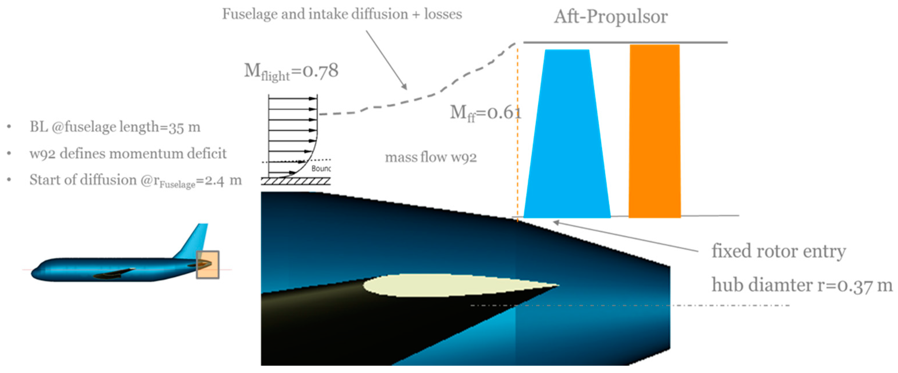
4.1.2. Power, Thrust Split and Aft-Fan Inlet Momentum Deficit/BLI Impact

As highlighted at the beginning of this paper, it is almost impossible to reliably quantify the average incoming momentum deficit to the aft propulsor, defined as:
[ v 0 , B L I w 92 , B L I v 0 w 92 ] / ( v 0 w 92 ) ,
and being induced by the fuselage boundary layer. To somehow consider this uncertainty in a sensitivity study, only the corresponding average velocity deficit v 0 , B L I was varied at given power input, and hence, mass flow rate w 92 , B L I = w 92 at constant flight velocity v 0 . This was done regardless of the physical achievability, and solely in order to investigate its effect on uninstalled SFC. At this stage, no detailed information regarding the shape of the boundary layer was needed, and in a first approach, only a small number of power-extraction levels and FPR were considered. The impact of this artificial variation of inlet momentum by specifying the corresponding average inlet conditions of the aft-fan only is shown in Figure 8a at different levels of power extraction PWX48 at constant FPR, and in Figure 8b for different aft-fan pressure ratios at constant PWX48:
The offset at zero momentum deficit, reflecting a better performance of all cases with aft propulsion compared with the baseline scenario, in general stems from improved propulsive efficiency of both, the main engine fan and aft-propulsor performance, as it will be explained later in this section. It is evident in those results that a rather high amount of power input is needed in order for the aft propulsor to substantially contribute to a reduction in SFC due to both, the BLI effect, as well as the generally higher levels of propulsive efficiency because of its lower FPR (compared with the main engine). The respective sensitivity between PWX48 and the momentum deficit is non-linear, and at a given theoretical momentum deficit, the additional SFC benefit increases with increasing aft-fan power. However, at given FPR, the aft-fan grows in diameter when increasing PWX48, and hence, the amount of achievable ingested boundary layer becomes smaller and almost cancels out any additional, BLI-related SFC benefit. In the figure, one vertical line defines the resulting inlet momentum deficit as calculated with flat-plate BL theory and can be related to the respective PWX48 or FPR sensitivity line by the same line style. The intersection of the two lines (vertical flat plate BL momentum deficit lines and PWX48 or FPR sensitivity lines at varying inlet momentum deficit) denotes what is, under the given assumptions, considered an achievable configuration. Those intersections are highlighted by the light grey markers. It is important to notice that at constant levels of power extraction, the fan mass flow rate is nearly constant and independent of the inlet momentum deficit. Connecting the intersecting points yields the light grey line, which suggests that further increasing the power input to the main fan at given FPR has no further benefit for the SFC, since the beneficial impact from ingesting the boundary layer becomes smaller and smaller with increasing mass flow rate/tip diameter. Subsequently, based on those results, a choice for the amount of power extraction has been made at PWX48 = 2000 kW, and the impact of varying aft-fan FPR has been investigated in the same fashion. Here the sensitivity of the BLI effect seems generally smaller in terms of uninstalled SFC benefit, but the results for the achievable configurations as denoted again by the light grey lines clearly suggest an optimal region of FPR at given power input. This optimal range is not driven by the aft-fan component efficiency (which was fixed for this particular study as will be discussed later), but rather by a trade-off between the beneficial effect of increasing the incoming momentum deficit and an overall lower level of propulsive efficiency at higher FPR. To further clarify the aforementioned observations, only the achievable configurations from both sensitivity studies are plotted together in Figure 9a. A quadratic fit, indicated by the light grey lines, was chosen to anticipate the behavior in between the calculated points, which is merely being used to illustrate the different characteristics of the two sensitivities (constant power extraction vs. constant FPR) rather than deriving an—at this point—still unknown optimum and detailed progression. The existence of an optimum will be derived later in this section based on refined data with more points considered, allowing to avoid any interpolation or anticipation of missing data. However, the almost asymptotic behavior of the PWX-sensitivity towards higher values of power input at the system level can be assumed (solid black lines), as well as the range of a potential maximum SFC benefit with varying FPR (dashed lines).
Splitting the overall aft-fan efficiency in transfer and propulsive efficiency (see Equations (10) and (11)), as shown in the right part of Figure 9b, it is possible to further explain both trends: At constant FPR and varying PWX48, the increase in jet velocity is solely driven by the incoming velocity deficit v 0 , B L I in a linear fashion, and w 95 and PWX48 scale in the same way, hence, their dependency is cancelled out. This leads to an almost linear dependency between transfer and propulsive efficiency. On the other hand, when varying the FPR at a given level of PWX48, the jet velocity of the aft-fan is not only driven by the incoming and BLI-related velocity deficit, but also by the FPR, which increases the jet velocity at higher FPR. At given and constant relative duct losses dPqP, increasing the FPR leads to an increase of the effective component efficiency [23]. As shown and discussed in the given reference, an increased FPR reduces the relative impact of dPqP on nozzle total pressure, and hence, increases the ideal velocity v 95 , i d . Looking into the definition of the transfer efficiency (15), this directly translates into higher levels of transfer efficiency with increasing FPR. As a result, one can observe a non-linear behavior of the aft-fans’s transfer and propulsive efficiency with a presumed optimal overall efficiency, and hence, lowest ΔSFC in the region of FPR ≈ 1.3, yielding the best compromise between an increased transfer efficiency at higher jet velocity levels and retaining high levels of propulsive efficiency for both, aft-fan and the main engine. In order to better quantify the optimal FPR for a maximal benefit in terms of uninstalled SFC, a refined sensitivity study was carried out subsequently for three different power extractions and a variety of FPR, and the results are shown in Figure 10. The dependency of the inlet momentum deficit here was removed by only considering achievable configurations and applying the corresponding momentum deficit for each point individually. The results suggest an optimal value of approximately FPR ≈ 1.27 for both cases PWX48 = 2000 kW and PWX48 = 2800 kW, and, as discussed before, a shift of the optimal FPR towards smaller values at lower levels of power as indicated by the white dashed lines. Again splitting up the aft-level performance into propulsive and transfer efficiency, the aforementioned sensitivities are visualized in Figure 11 for the aft-fan first: The transfer efficiency is almost constant at given FPR with only very minor differences in LPT efficiencies. Hence, transfer efficiency is almost independent of the levels of power-off takes (see Equation (11)), while the propulsive efficiency is a function of both, power off-take and FPR (Equation (10)) reaching its maximum towards lowest values of FPR and power off-takes with highest values at low FPR. Here it is interesting to note that the propulsive efficiency at constant FPR decreases with increased power inputs PWX48, which is directly associated with a decreasing BLI benefit, due to the aft-fan’s larger dimensions.
Figure 12 shows the same results for the main engine. The trend for the transfer efficiency (Equation (7)) is exactly the opposite as for the aft-fan and shows a dependency mainly on the level of power off-take and only a very small dependence on aft-fan FPR, due to minor changes in core efficiency levels and a different and BLI-dependent thrust split. The sensitivity with power off-take, however, is rather small with a difference of 1.3% between the minimum and maximum level of PWX48, due to almost identical levels of gas turbine core efficiency at all levels of PWX48. The propulsive efficiency yields the opposite trend, here high power off-takes results in higher levels of propulsive efficiency, due to higher thrust contributions from the aft-fan, resulting in a lower FPR of the main engine, and as a consequence, higher levels of propulsive efficiency. Again, the range of variation is relatively small with a 1.9% maximal difference between highest and lowest propulsive efficiency and in general, a gain in propulsive efficiency is traded for a decrease in transfer efficiency in almost the same manner. The results also suggest a very low overall dependence on aft-fan FPR and the dominant quantity defining the main engine performance is the power off-take; the power off-take itself is enabled at constant gas turbine core efficiency levels, OPR, T4 and pressure ratio split PRn by adjusting the core mass flow rate, compressors pressure ratios, and pressure drop over the LPT. The coupling with the bypass flow at given inlet mass flow rate w 2 is then achieved by varying the bypass ratio, as well as the main engine fan pressure ratio to meet overall thrust requirements at the given jet velocity ratio. At the system level, all of the aforementioned trends yield the results, as shown in Figure 13: Both, transfer (Equation (15)) and propulsive efficiencies (Equation (14)) have almost opposite trends, with higher levels for the propulsive efficiency at increasing levels of power off-take and only a small remaining dependency from aft-fan FPR and a similar, but opposite trend for the transfer efficiency: Here the highest levels were observed at higher values of aft-fan FPR and towards low power off-takes. The resulting products of transfer and propulsive efficiencies of the aft-propulsor (a), the main engine (b) and the system (resulting from a mass flow weighed combination of both, aft-fan and main engine, (c)) are finally shown in the respective diagrams of Figure 14 (see also Equations (6), (11) and (15)). Here it can be seen again how beyond a certain (aft-fan FPR-dependent) level of power-extraction there is almost no additional SFC benefit (c) due to opposite sensitivities of aft-fan (a) and main engine (b) propulsive efficiency and a diminishing additional BLI benefit towards increasing aft-fan dimensions. Moreover, the effect of the main engine seems of lower importance, since the levels of overall efficiency are very close to each other, with a maximum difference of approximately 0.6% and maximum values at highest aft-fan power off-takes, and hence, lowest main engine FPR. The overall system efficiency, and hence, SFC benefit is mostly driven by the aft-fan, of which a significant thrust contribution is needed to translate into an overall SFC benefit.

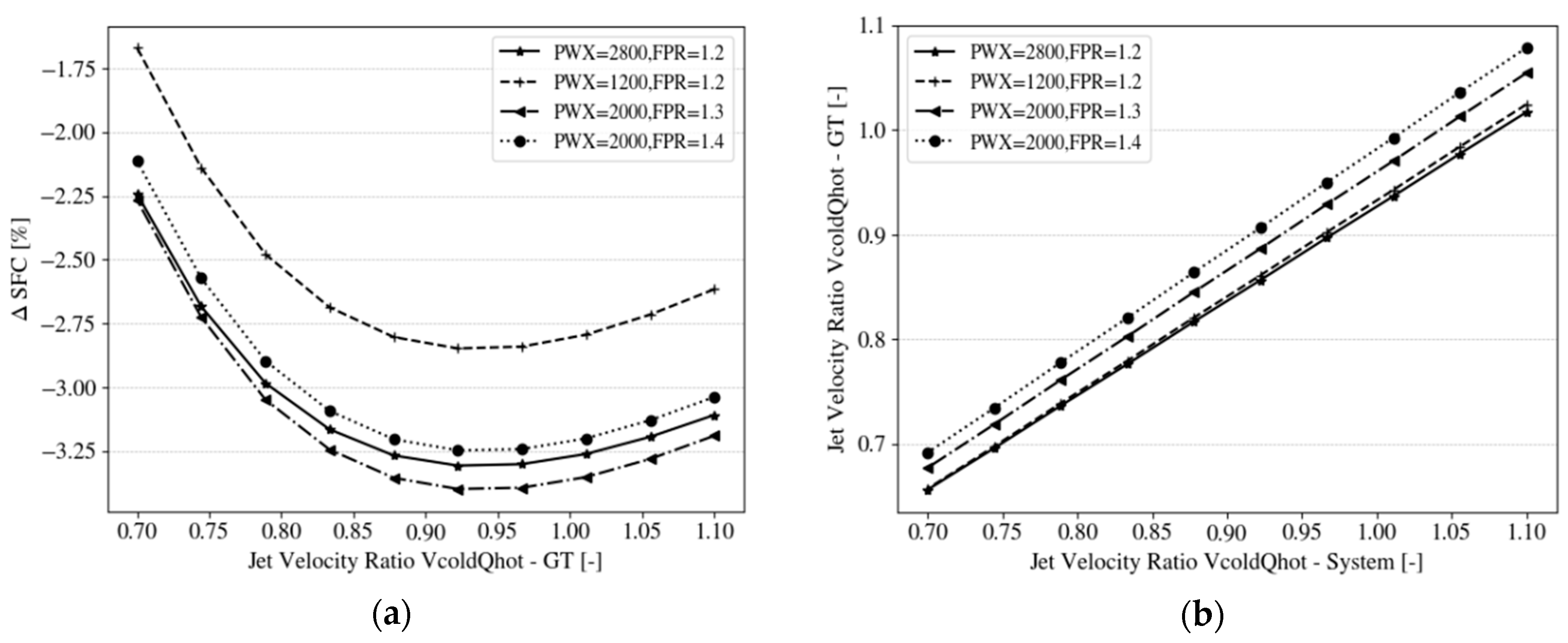
4.1.3. Gas Turbine and Aft-Propulsor Jet Velocity Ratio Impact

The results discussed in the previous chapter were all obtained for fixed values of the gas turbine jet velocity ratio VcoldQhot, and in this chapter, its impact shall be discussed. In general, the jet velocity ratio can be considered for the gas turbine and the aft-fan separately, as well as at a system level, and its choice has a direct impact on the overall efficiency (see Section 4.1). In a subsequent sensitivity study, the respective jet velocity ratio was varied within a range of [0.7 … 1.1], and the performance was evaluated for four selected cases (indicated by the markers in the previous section: [FPR = 1.2, PWX48 = 1200 kW], [FPR = 1.2, PWX48 = 2800 kW], [FPR = 1.3, PWX48 = 2000 kW], and [FPR = 1.4, PWX48 = 2000 kW]) with the achievable momentum deficit of the respective configuration being imposed; the corresponding results are shown in Figure 15. One of the main conclusions from Figure 15a is that the gas turbine jet velocity ratio optimization (location of the uninstalled SFC-benefit maximum) seems not to be influenced by the level of the aft-fan power off-take and aft-fan FPR; as a consequence, one can keep the BPR optimization for the bypass side as per traditional conceptual design practice. Based strictly on the cycle design, the optimum SFC occurs at a velocity ratio of about 0.925, but considering system level design aspects, such as mission-based block fuel rather than SFC, an optimum value of velocity ratio would be expected to be lower than this and closer to 0.9. The details of this system level design trade-off are beyond the scope of this work, but details can be found in reference [6], including the rationale as to why slightly moving away from the optimum towards lower values is more favorouble when also considering mission-based block fuel; for further analysis herein a value of VcoldQhot = 0.9 was chosen. The results also suggest that the system jet velocity ratio is influenced by choice of aft-fan FPR, but not by the amount of power transferred to it, and the relation between system and gas turbine jet velocity ratio is linear in nature (Figure 15b).
To complement those results, a similar study was carried out by varying inlet momentum deficit for three different levels of aft-fan FPR (here only aft-fan FPR was varied, because the system jet velocity ratio was independent of power extraction as highlighted already); the results are shown in Figure 16 with the achievable configurations again denoted by the colored markers.

4.2. Cases Downselection

Based on the sensitivity study discussed in the previous chapter, four cases were downselected in order to allow for the conceptual design of the aft propulsor and discuss the resulting component performance and design implications. Those cases comprise two different power extraction levels at constant FPR and two different aft-fan pressure ratios at a constant level of power extraction:
  • FPR = 1.2 and PWX48 = 1200 kW,
  • FPR = 1.2 and PWX48 = 2800 kW,
  • FPR = 1.3 and PWX48 = 2000 kW and
  • FPR = 1.4 and PWX48 = 2000 kW.
The cases were chosen because they all had comparable (uninstalled) SFC benefits, but were expected to lead to substantially different designs of the aft-fan.

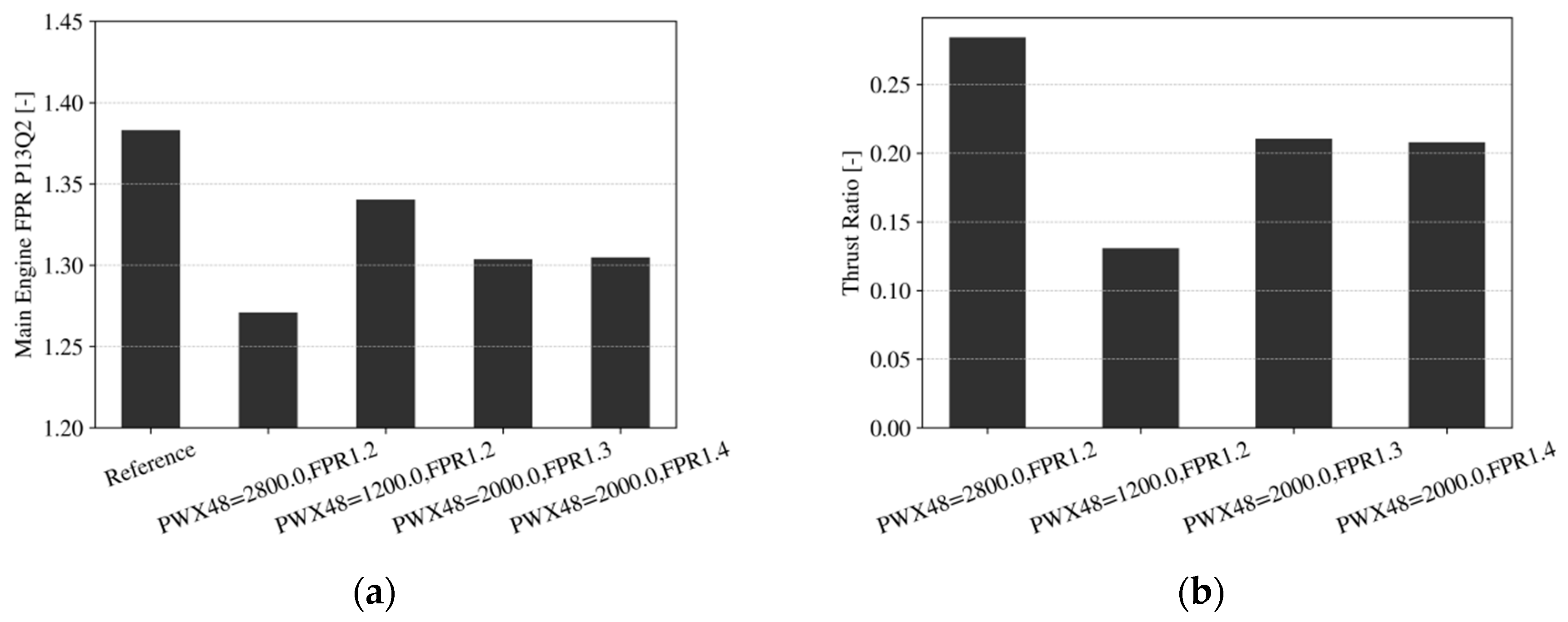
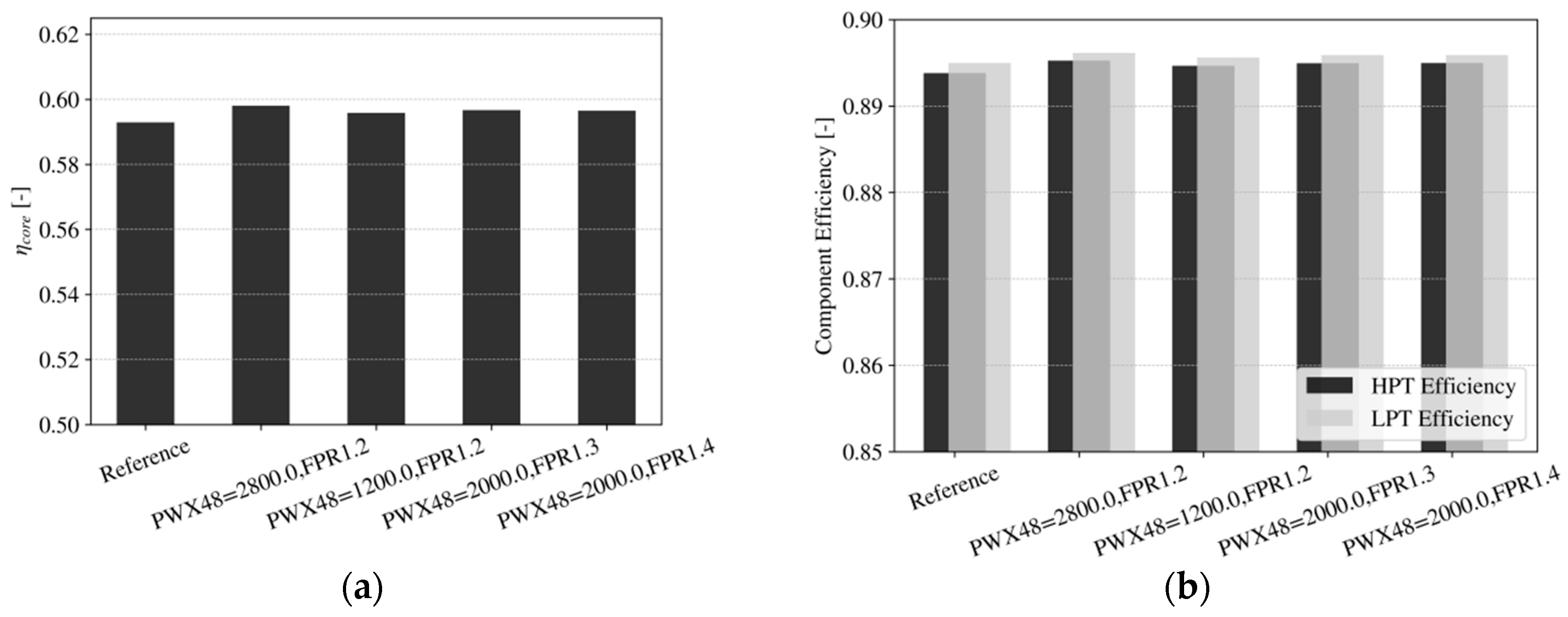
4.2.1. Choice of Main Gas Turbine Cycle and Resulting Engine Performance

Before discussing the design of the aft-fan in the next chapter, the resulting performance of the main engine shall be summarized for all four cases. One assumption, the consequences of which were not discussed yet in detail, was that the main engine was operated at constant mass flow rate w2. With increasing thrust contribution from the aft-fan, the thrust requirement of the main engine was reduced, allowing for a lower FPR of the main engine fan and corresponding operation at higher levels of propulsive efficiency (and compromised transmission efficiency). The values for all four cases in direct comparison with the baseline engine are shown in Figure 17 at Cruise conditions. One example underlining the constant gas generator performance for all cases is shown in Figure 18, yielding almost identical levels of core efficiency, as well as High-Pressure Compressor (HPC) and LPC component efficiencies (minor differences stem from the fact that the design point of the engine was Top-of-Climb, and the shown results at Cruise condition, hence, are at off-design). This was achieved by the application of the multi-point synthesis matching scheme. All in all, this resulted in a more or less SFC neutral operation of the main engine and the SFC benefits at a system level stem almost exclusively from the aft-propulsor as discussed in the previous Section 4.1.1.

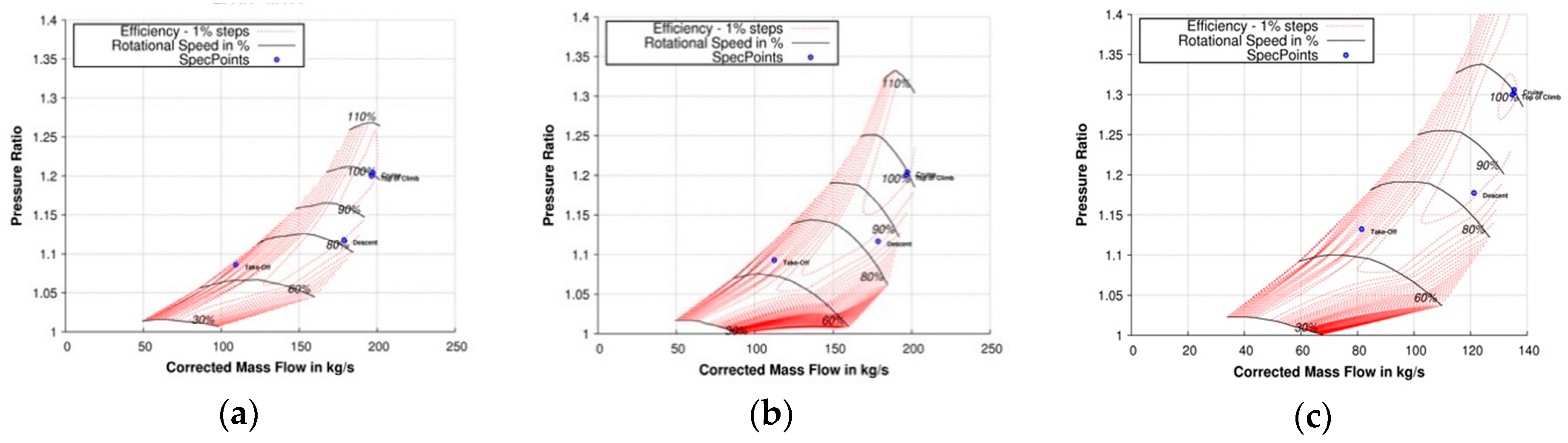
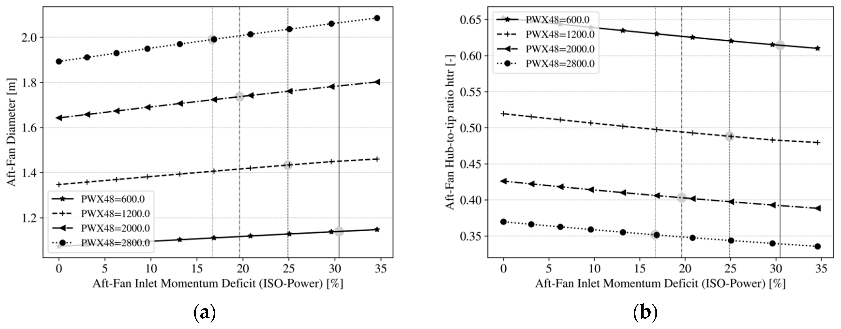
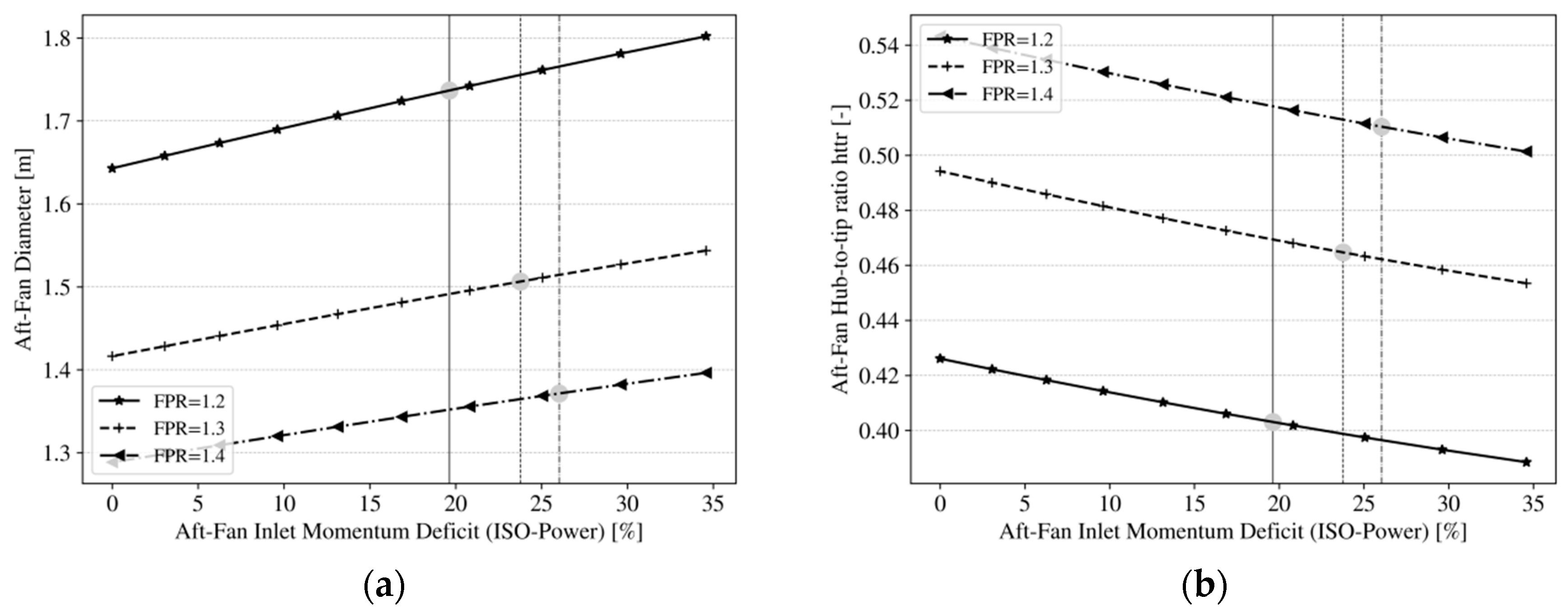
4.2.2. Aft-Propulsor Design Rationale and Top-Level Design Parameters for Downselected Cases

The main assumptions for the aft-fan conceptual design, which were equally applied to all cases (BLI and non-BLI) at design conditions, are as follows:
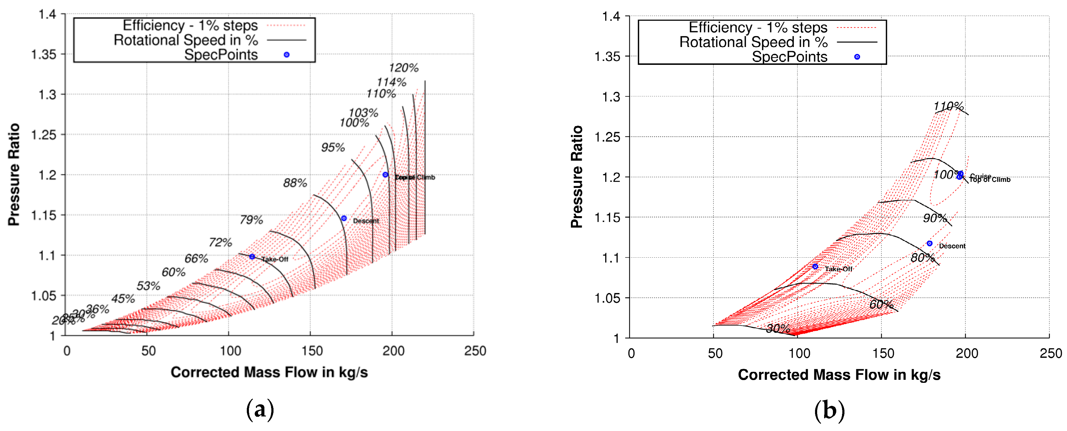
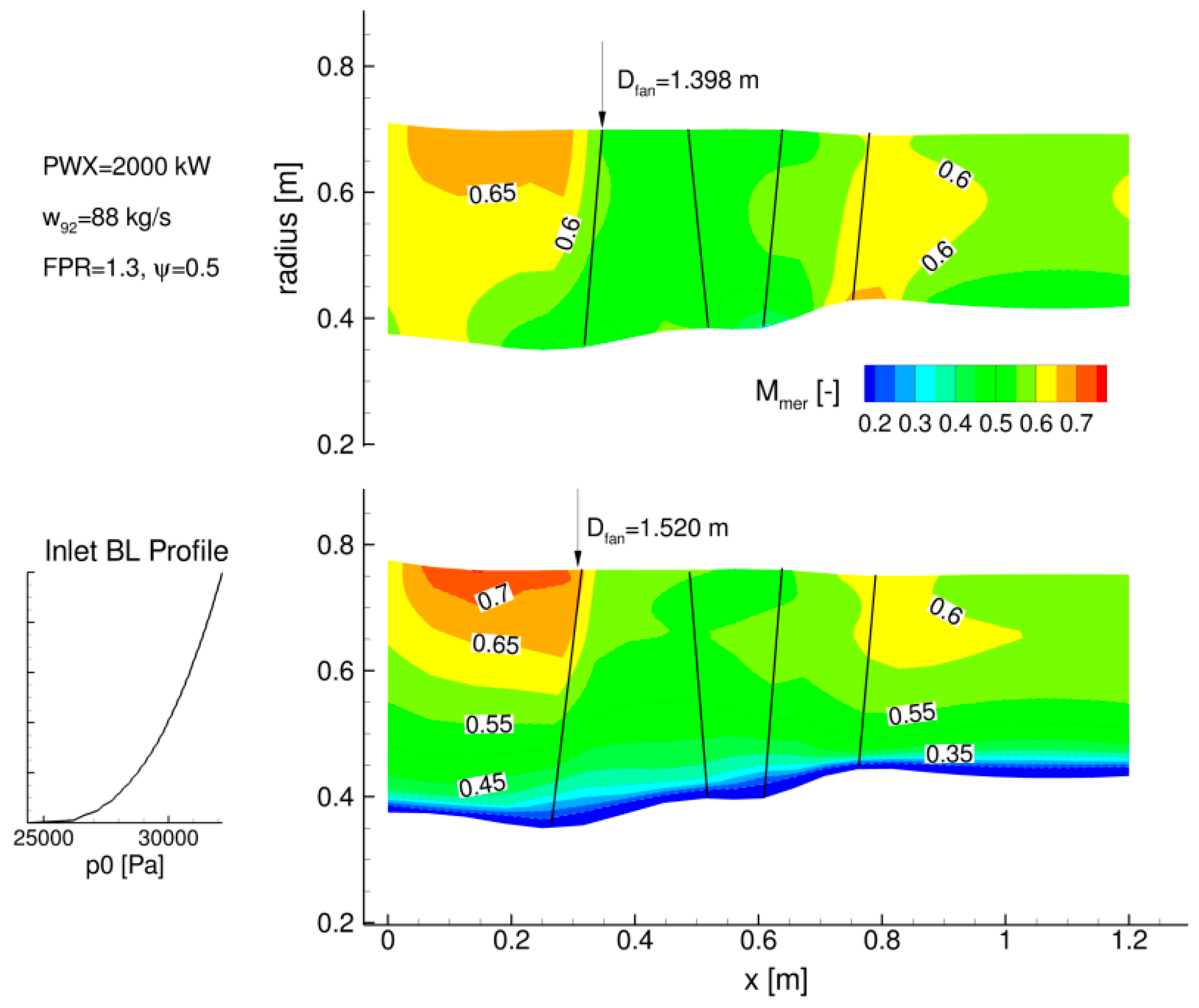
  • Constant meridional Mach number at fan face: Maff = 0.61 (this value is based on experience, reflecting trends in both, current and future engine designs, and was chosen in order to allow for high fan efficiency levels, sufficient flow capacity and compactness of the engine, see Reference [24] or Reference [25]). For the BLI-cases, where the resulting Mach number at fan entry at a given mass flow rate is inherently not constant over the span, an average value of Maff = 0.61 was targeted when sizing the aft-fan in order to ensure a certain coherence in the design strategies. Further design assumptions were:
  • Limitation of the (local) blade diffusion factors for both, rotor and OGV: Diffusion factor (DF) < 0.45, as well as respective de-Haller numbers: de-Haller > 0.7; those values were chosen based on common textbook recommendations [26,27,28], as well as in-house design experience [24];
  • Swirl free outflow from the OGV;
  • A loss-driven limitation of the mean OGV exit Mach number (Ma < 0.65);
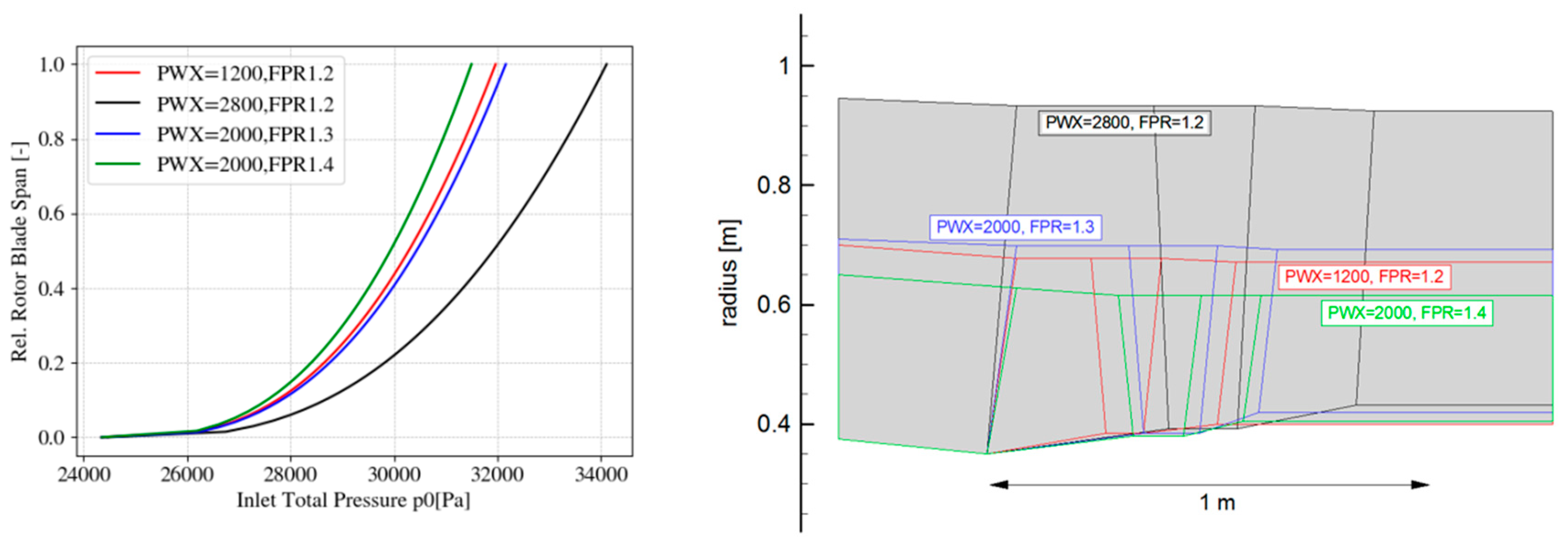
  • Fixed hub radius at the rotor leading edge: r = 0.37 m.
A final assumption made for the fan design involves the work coefficient Ψ as the ratio of the fan rotors’ average change in total enthalpy Δ h t over u m e a n 2 . Using eulers’ turbomachinery equation, this can also be expressed as the (mean) flow turning c u , 2 , m e a n over the circumferential velocity u m e a n = r m e a n · R P M :
Ψ = Δ h t u m e a n 2 = c u , 2 , m e a n u m e a n
This parameter reflects whether the work input to achieve a given level of FPR is realized at higher levels of flow turning (higher values of Ψ) or higher tip speeds (higher values of u m e a n , and hence, lower values of Ψ). It essentially comes down to balancing shock losses at high levels of tip speed and viscous losses, due to flow turning. Typical choices of Ψ can be found in References [24,25], and in this study the resulting tip speed was made based on different values for Ψ = ( 0.4 / 0.5 / 0.6 ) , reflecting different design philosophies with lower and higher levels of rotor tip speed and resulting turning requirements.
Aft-fan off-design performance was not explicitly addressed in all design efforts, but to some extent, considered implicitly by choice of the values for maximum DF. Combining those assumptions with the given top-level parameters from the cycle for all four cases, one can first define the dimensions of the fan rotor in terms of its diameter and hub-to-tip ratio at given FPR and mass flow rate w92 (as resulting from the level of power off-take); the respective values for all four cases can be extracted from Figure 19 and Figure 20. Two major impacts on the fan design can be seen in this figure: Firstly, by fixing the hub diameter at rotor entry, the values for the hub-to-tip ratio vary substantially with changing fan diameter; hence, a given design cannot be scaled to another PWX48 level. Secondly, because of constant power input to the aft-fan, its diameter increases with increasing incoming momentum deficit because the momentum deficit is directly associated with a total pressure loss. Hence, at lower levels and radial variation of the aft-fan inlet total pressure and constant mass flow rate, the aft-fan diameters must be adjusted to those conditions in order to meet the given (average) fan face Mach number; this was done in an iterative manner for the BLI cases.
The boundary conditions in terms of the inlet total pressure profiles, resulting from flat plate theory at a given mass flow rate and fan dimensions, are shown in Figure 21 (left). Those profiles were directly imposed as a boundary condition for the streamline-curvature method by mapping the resulting profile with the entry area and respective hub and tip radii. This mapping procedure was a compromise since it is not fully consistent in terms of momentum conservation (for more details see Reference [9]), but is practically applicable and is believed to allow for an assessment of the major implications the incoming BL has on the fan design. The other boundary conditions being imposed were a constant total temperature T0 at given flight velocity and altitude, zero inlet swirl and radial flow angles as taken from the annulus lines.
Apart from the concrete design rationale as being applied to each configuration, a matrix for the choice of other different major fan design parameters was set up and realized to systematically study the effect of:
  • Corrected tip speed (or respective work coefficient Ψ);
  • Hub-to-tip ratio;
  • Different radial total pressure profiles of the rotor (quasi free-vortex and bound-vortex);
  • Major annulus design parameters/contraction.
On the aft-propulsor’s BLI and non-BLI performance. This matrix, along with the resulting values of all parameters, is shown in Table 3. It was implemented by firstly design a fan in a conventional fashion and not taking into account the BLI effect (hence, without any radial pressure profile), then impose the respective boundary layer profile and assess the resulting performance and finally update the initial design to account for the BLI effect and recover the initial performance (if possible).

4.2.3. Aft-Propulsor Baseline Designs and Non-BLI Performance (Dfan for BLI Cases Adapted to Meet Target Fan-Face Axial Mach Number at Given Mass Flow Rate)

The designs and respective performance of the four baseline aft-propulsors are summarized in Figure 22 in terms of their span-wise distributions of the major performance indicators. All designs were made and assessed at altitude conditions, firstly without any inlet total pressure profile being imposed (non-BLI). A similar radial total pressure profile over the rotor was introduced into all designs, the mass average of which results in the respective design target FPR within a range of ±0.5%. A work coefficient of Ψ = 0.5 was chosen for the lower FPR designs (1.2 and 1.3) and Ψ = 0.4 for the higher FPR of 1.4 in order to select the respective rotor tip speed. The radial profiles, in general, suggest a comparable performance of all four designs and the resulting stage efficiency was close to 94% for the cases with FPR = 1.2 and FPR = 1.3 and at 93.3% for the case with the higher FPR = 1.4. This loss in efficiency at higher FPR stems from a higher blade tip speed at given work coefficient, which well exceeded sonic conditions and the resulting shock-induced losses are associated with this drop in stage performance. The demonstrated radial distributions well reflect the design rationale in terms of limiting the maximal blade diffusion numbers (shown as blue dashed lines) in both blade rows. The rotor hub section is less loaded typically in terms of blade diffusion number; this is driven by the high de-Haller resulting from high turning requirements at the hub near profiles, where circumferential velocity typically is low, due to the low hub radius and a high level of flow turning is needed to meet the given pressure ratio; hence, rotor de-Haller numbers at the hub are close to 1 or even higher, indicating a blade row with very low flow diffusion or even flow acceleration. In the designs, it is interesting to highlight one of the implications as imposed by one of the aft-propulsor geometric constraints: The fixed hub entry radius resulted in different hub-to-tip ratios for all cases, varying between 0.375 and 0.55. In particular, the cases with an equal FPR of 1.2, but different hub-to-tip ratios (httr) allowed for highlighting the influence: At higher hub-to-tip ratios the flow turning requirements of the hub section of the rotor decrease at given rotor tip velocity by up to 5° (at given work coefficient Ψ, the rotor corrected tip speed is actually also a function of the httr, but its influence is considered of minor importance for the given conclusions [24,25]), which is of importance when imposing the boundary layer profile.

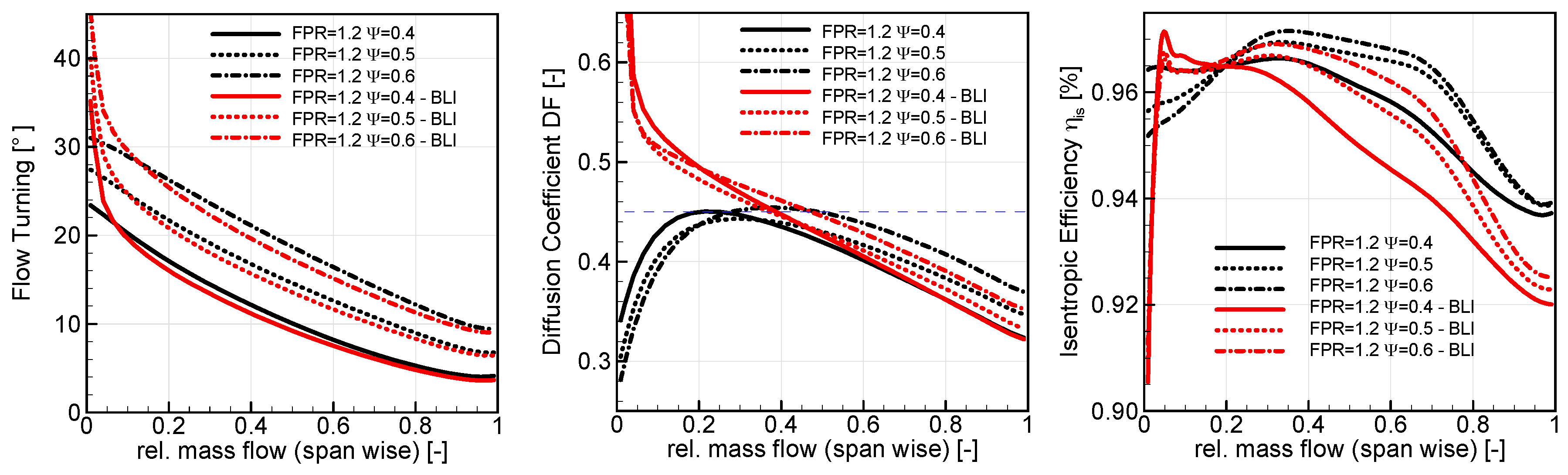
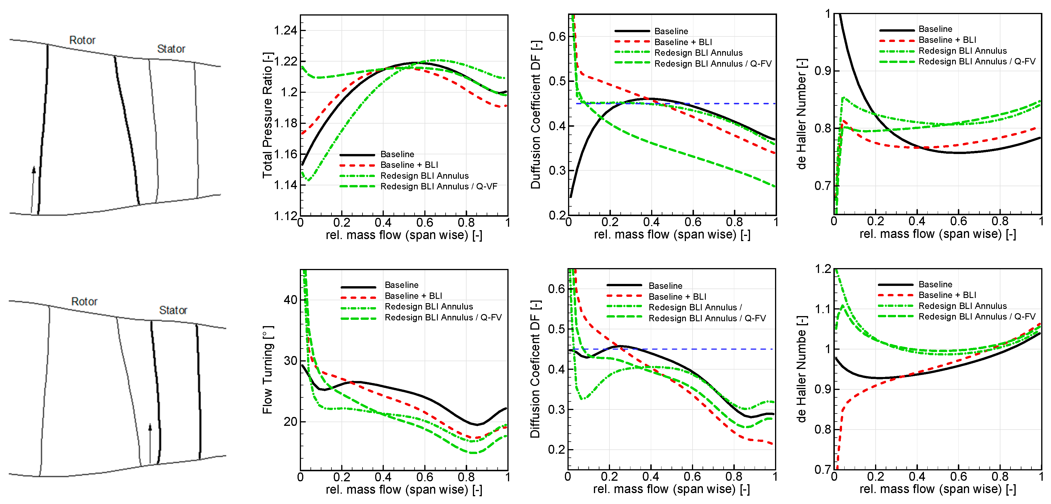
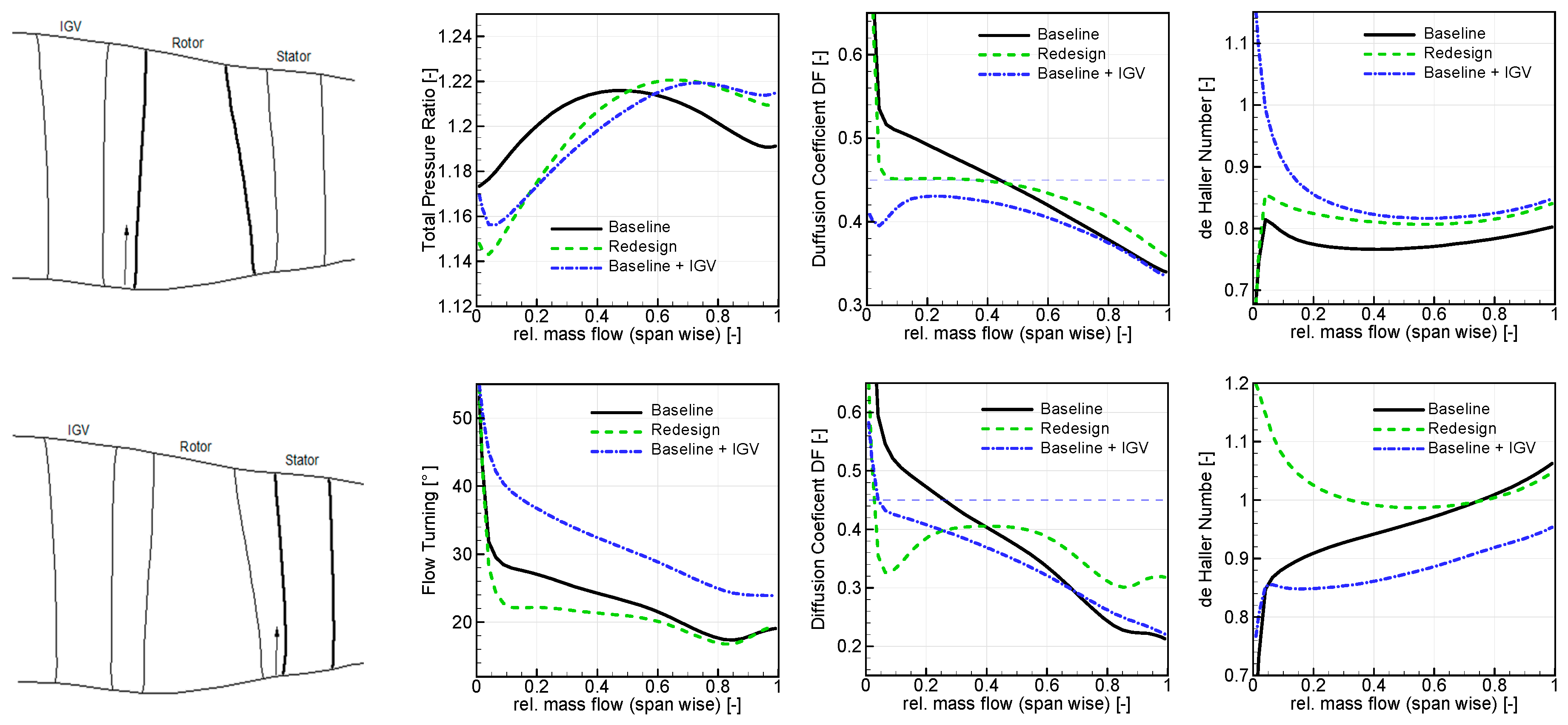
4.2.4. BLI Effect on Aft-Fan Performance and Design Update of Selected Cases

In a next step, the influence of the inlet boundary layer profile on the blade row and stage performance shall be discussed, as well as design updates to better accommodate the incoming boundary layer shall be also introduced and discussed:

BLI Effect on Baseline Design

To firstly highlight the general effect of the BLI, the distribution of the meridional Mach number Mmer is shown in Figure 23 for the baseline and the BLI case for FPR = 1.3: As one would expect, the low momentum region entering the fan stage near the hub translates into a very low Mach number (Mmer < 0.4); to meet the given mass flow requirements (which were identical for all cases as discussed in the context of the PWX sensitivity study), the meridional Mach number in the tip region was increased to meet the design target and limit the average Mach number at the fan face to the given values. To compensate for the low inlet total pressure ratio, the rotor tip diameter had to increase. As it turned out, it had to increase further as compared to the values provided in the previous chapter and stemming from the performance analysis with only average values of p0 to account for the actual radial distribution of the incoming total pressure.

Influence of Corrected Tip Speed on BLI Performance

Since one of the most important choices to be made was the rotor corrected tip speed for a given FPR, the effect of different values thereof shall be discussed next, considering the effect it has on both, BLI and non-BLI performance. The results will be discussed by example of the case with FPR = 1.2 and a reference hub-to-tip ratio of 0.5, the results of which are shown in Figure 24 for the aft-fan rotor only. The overall increased level of required flow turning with decreasing work coefficient or respective higher tip speeds is shown in the right diagram of the figure. In addition, two main observations can be made in this context: First of all, applying the inlet boundary to the baseline design will lead to a failure of the hub sections, due to excessive loading. This is caused by the increased turning and flow diffusion requirements at low levels of axial velocity as induced by the BLI, resulting in values for the diffusion factor DF well above the required limit up to a radius covering 40% of the total mass flow. Essentially this effect is the same for all given designs and levels of Ψ. However, the effect on rotor isentropic efficiency seems well dependent on the choice of its tip speed and the rotor efficiency loss, due to the BLI effect seems to get smaller at lower tip speeds.

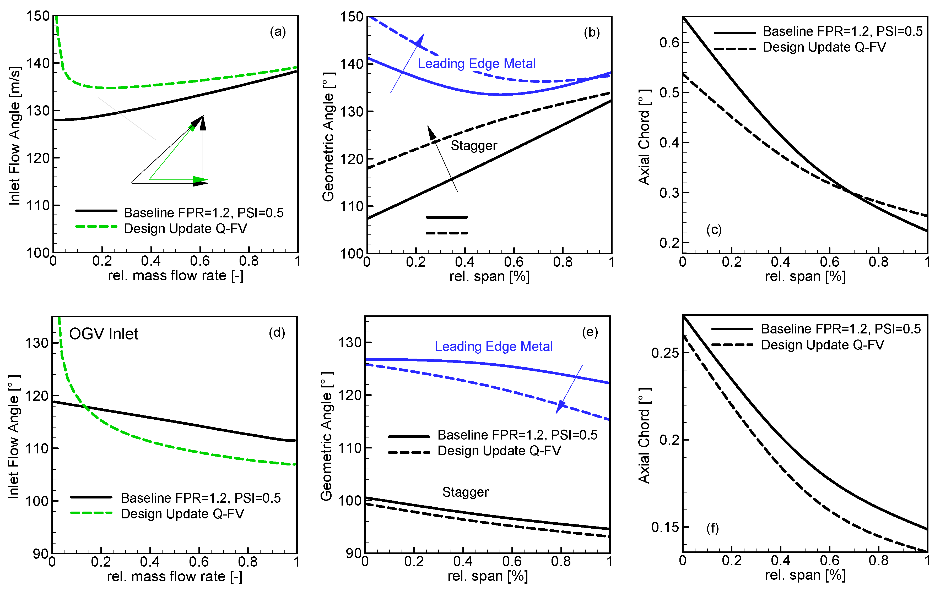
BLI Design Update (Conceptual)

After having discussed the BLI effect on the baseline cases, ways to compensate for the negative effect of the incoming boundary layer profile, and hence, to design an operational aft-propulsor under the given assumptions shall be investigated. This design update was made at the conceptual level and under the same assumptions and according to the rationale highlighted at the beginning of this chapter. In the same way as the baseline design, it was made within several manual iterations which were possible thanks to extremely low turnaround times of the SLC method. The main design parameters that were used are the annulus lines in the region of the rotor and the OGV, as well as blade row meta parameters, such as axial chord, resulting from the definition of the blade rows’ leading and trailing edge. Furthermore, re-distributing the radial pressure profile as imposed by the rotor was used as an additional means for the rotor to better cope with the incoming flow distortion. This was realized by retaining an average value of FPR as requested by the cycle. At this stage, the designs iterations described here do not require any knowledge of the actual blade shape.
The design update will be done again by analyzing one selected case at FPR = 1.2, PWX48 = 2000 kW and Ψ = 0.5. Figure 25 shows results for the four designs in a direct comparison: The solid black lines denote the baseline case without BLI, and the dashed red lines show the BLI performance of the same configuration. In addition, two more cases were introduced: One where the annulus was used to introduce additional (local) contraction close to the rotor and OGV hub in order to limit the peak diffusion values below the given threshold. With the BLI imposed, an overall radial imbalance is essentially retained, but the hub sections are unloaded and are expected to deliver the requested flow turning. The other strategy involves updating the span-wise rotor total pressure distribution. As also discussed in Reference [29], increasing the total pressure ratio near the rotor hub may support balancing the flow distribution and lead to a more homogenous total pressure profile (and hence, velocity profile) at the rotor and OGV exit. The authors suggest a “hub strong profile” with a maximum total pressure ratio near the hub, for which they were able to achieve an almost constant total pressure distribution at OGV outflow. In this study, we introduced a quasi free-vortex design with an almost constant pressure distribution over the rotor (green dashed lines in Figure 25). It is considered quasi free-vortex, due to the nature of the given methodology: Rather than imposing a constant work coefficient, which technically would lead to a free-vortex design, a nearly constant total pressure profile was imposed and the resulting local work coefficient emanates from the corresponding level of FPR and resulting efficiency level (which resulted from the profile pressure losses given by the profile database being part of the streamline curvature approach). This design also led to a configuration accounting for the incoming boundary layer at acceptable levels of blade row diffusion. Further increasing the hub total pressure ratio to a fully “hub strong profile”, in order to completely harmonize and balance the radial flow distribution, was not considered here for mainly two reasons: First of all, it is believed that further loading the hub sections would require a significant increase in tip speed (in particular for the lower hub-to-tip ratio cases) which might compromise performance and the risk of losing stall margin seems high. Moreover, if this were to be realized, the tip sections would become more and more unloaded and less efficient (or the respective chord would be excessively small to maintain the same DF over the entire blade and compensate for this effect). Both seems not reasonable, but as stated before, more CFD based design and optimization efforts to study all trade-offs are necessary e.g., as performed in [30].

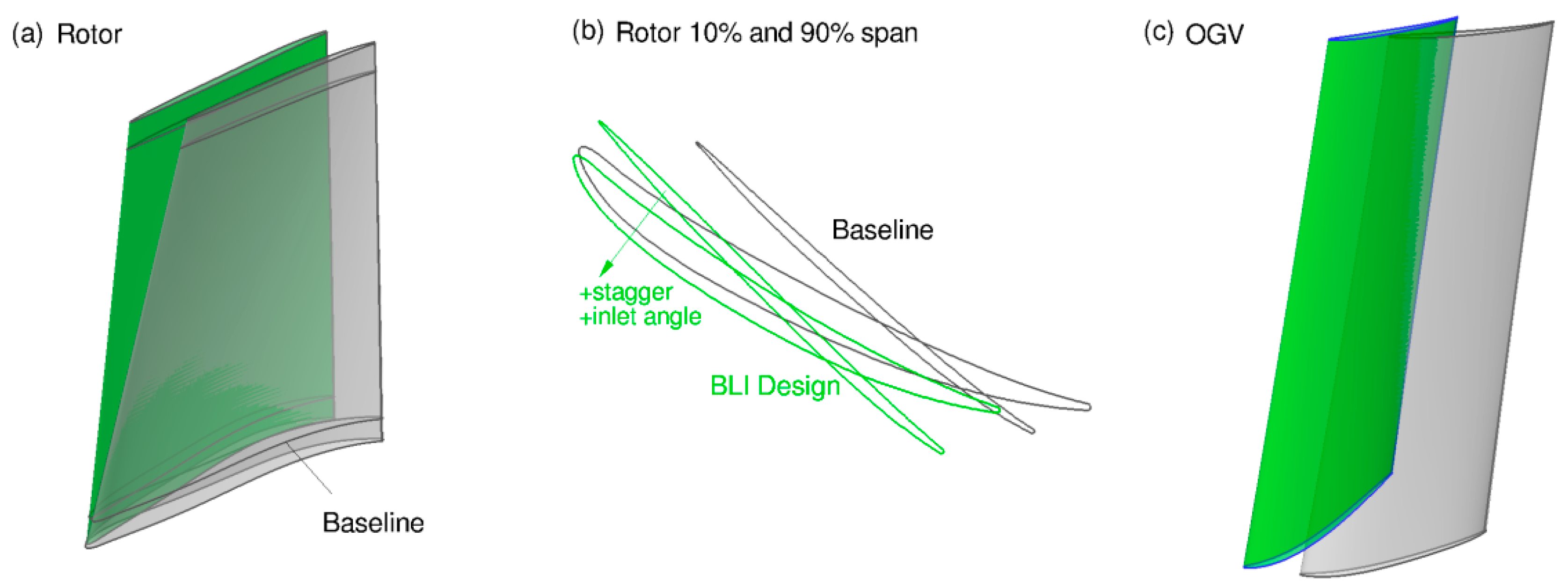
BLI Design Update—Resulting Geometric Changes

Since a detailed blade geometry could be derived right away after running the SLC method by taking advantage of a pre-optimized profile database, the main changes in the aft-propulsor geometry to accommodate the incoming boundary layer will be described next by example of one selected case (FPR = 1.2 and Ψ = 0.5, quasi free-vortex (Q-FV) design, as shown in Figure 25). The basis of this was mainly the turning requirements, as shown in Figure 25, as well as and the respective inlet flow angles; those flow angles are shown in Figure 26a for the rotor and for the OGV in Figure 26d. The resulting near-hub velocity triangles are schematically shown for the rotor in Figure 26a, with the black arrows indicating a non-BLI and the green arrows the BLI scenario. The major effect of the incoming momentum deficit near the hub is the increased rotor inlet flow angle as compared with the non-BLI case. This can be seen in both, the resulting flow angles, as well as the velocity triangles. The corresponding profile sections were both, re-staggered and their respective inlet metal angle was increased, as shown in Figure 26b, with the trailing edge angles then resulting from given turning requirements and deviation levels derived from the loss correlations within the SLC method. The OGV, aiming to provide a swirl free outflow, predominantly experienced lower inlet flow angles with a strong gradient near the very hub, due to the shape of the boundary layer profile. Only parts of this were compensated for when adapting the respective metal and stagger angles due, as shown in Figure 26e. The resulting chord requirements, which were also adapted to limit the blade loading in terms of DF and de Haller number, are provided in Figure 26c for the rotor and in Figure 26f for the OGV.
The resulting 3D blade shape consists of profiles at different radial locations as selected from the existing database, based on the results from the SLC run at design conditions. In between the selected control profiles, which were stacked radially according to their respective center of gravity on the given stream line, additional profiles were created based on interpolation in order to describe the full 3D blade geometry within the given annulus lines. The resulting geometries of both, rotor and OGV, reflecting the aforementioned adaptions of local metal and stagger angles, are shown in Figure 27 for the non-BLI and the updated BLI design. Apart from the change in the profile shape as shown for a near hub and a near tip profile, the increase in annulus contraction for the BLI case to reduce the blade loading is visible in the 3D geometries. This blade geometry can be the very basis for a subsequent detailed and 3D-CFD based design (optimization) study which is needed to confirm the observed trends, particularly focusing in the endwall regions where the SLC method is not expected to provide the necessary level of fidelity. A 3D view of the aft-propulsor, including the nacelle, resulting from a study investigating the overall structural concept is shown in Figure 28.

BLI Design Update—Introduction of an Inlet Guide Vane (IGV)

Finally, a third way of compensating the detrimental effects of the inlet boundary layer profile and the resulting high flow turning requirements of the hub sections shall be discussed: This solution is essentially based on introducing an Inlet Guide Vane (IGV) upstream of the rotor. The motivation is that by introducing contra-swirl near the hub of the rotor, its flow turning requirements and hence, blade loading will be reduced, which may help to balance the performance in spanwise direction and reduce the risk of a compromised stall margin. The introduction of an IGV was further motivated by the fact that struts presumably will need to be introduced upstream of the rotor (see Reference [10]) and a structural-IGV, as already realized in the bypass duct within several studies, seems a worthwhile concept to be studied. In the present work, an almost linear swirl variation from approximately 20° near the hub to 0° close to the tip was chosen to be introduced by the IGV. The respective results are shown in the diagrams of Figure 29: The results for the baseline case with IGV were equally successful in limiting and balancing the rotor blade row diffusion in terms of DF, leasing to a functional rotor design from a performance perspective. However, the turning requirements of the OGV were substantially increased, which required for more blades to be introduced in order to limit the respective DF. This resulted in a loss in efficiency, which was further compromised by the OGV losses, resulting in a more than 2.5% loss in isentropic stage efficiency. Again, this needs to be assessed and confirmed in more detailed design studies involving methods with higher fidelity, but the trends are expected to support defining appropriate configurations, and hence, limit the number of detailed design iterations.

4.3. Overall Configuration Potential

In the previous chapters, the uninstalled SFC was considered as a main figure of merit in order to discuss the potential of the given configuration. Since it is expected that the added weight of both, the electrical system, as well as and the aft propulsor, together with the additional aft-fan’s drag, will significantly influence this potential, as well as change the ranking of the selected cases, the impact of both shall be discussed next. The main engines weight and drag change are not considered given the nature of the study, which kept the mass flow rate entering the main engine and hence, its diameter constant. Moreover, the change in overall mass distribution and associated relocation of the center of gravity of the aircraft, which will require changes on the aircraft design, are not being considered.

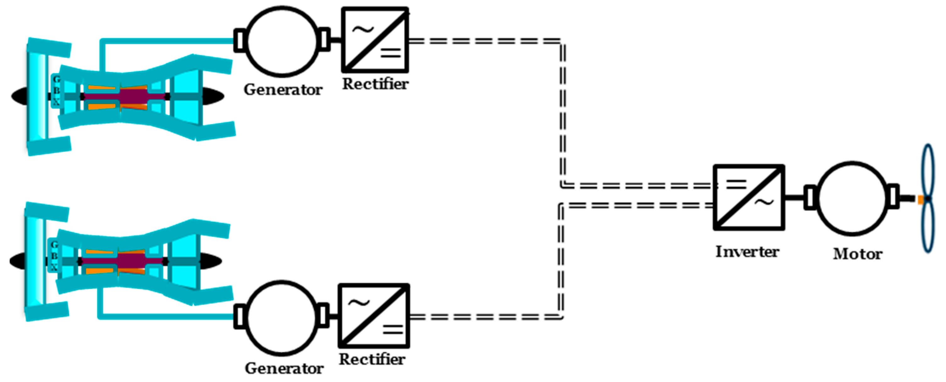
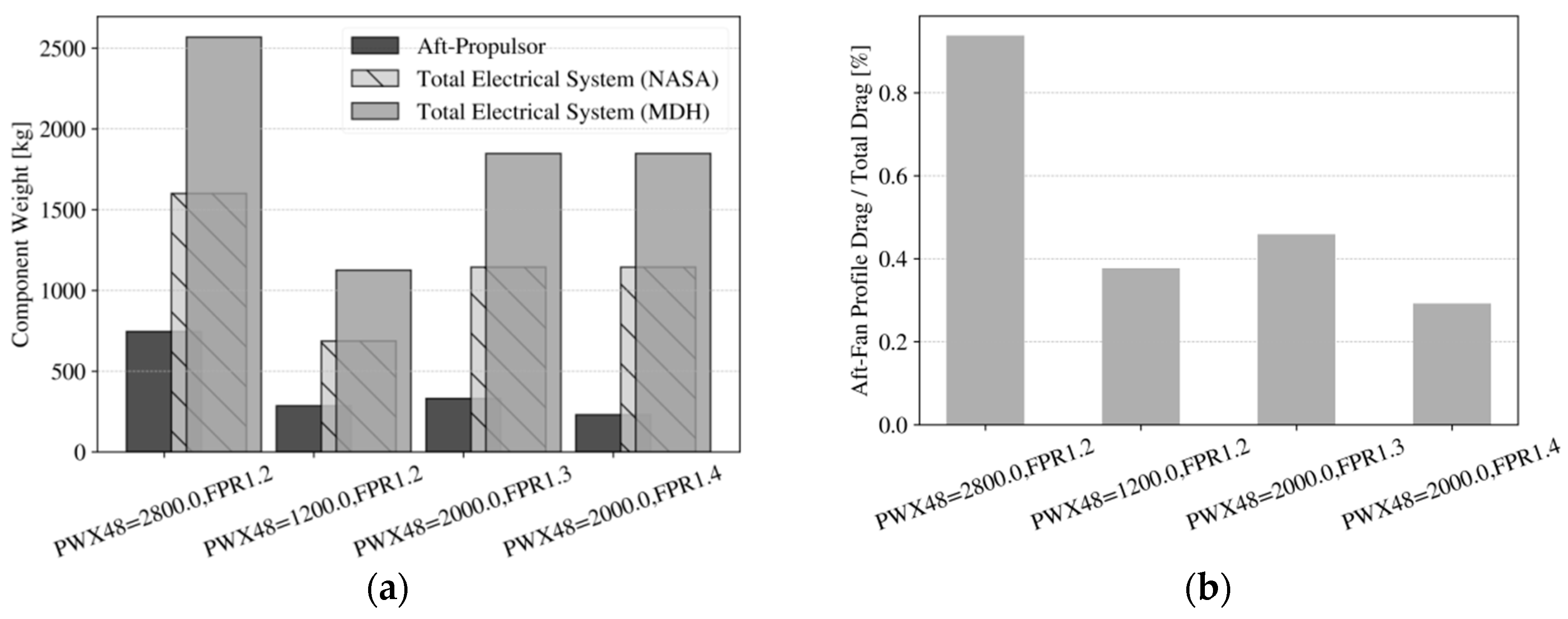
4.3.1. Electrical System Dimensioning

As explained under Section 4.1, one of the parameters, which will affect the overall propulsion system efficiency is the electrical drivetrain efficiency. If one ignores the weight impact from the additional electrical components, the conversion losses in the electrical drive system must be compensated by the benefits from the system efficiency improvement for the viability of the concept. In the above context, a thrust split ratio between the main engines and the aft engine would dictate the desired performance in the electrical drivetrain. Two performance parameters are vital for its performance: Specific power, and efficiency of the electrical drivetrain. A highly efficient and high specific power electrical drive system is desired for achieving best benefit from the hybrid operation. In order to predict the appropriate numbers for the aforementioned parameters in a timeframe finishing in 2035, a study was conducted. Few studies are found driven by NASA’s goal of achieving machine power density and efficiency @13.2 kW/kg and >96% and power converter power density and efficiency @19 kW/kg and >98%. Both cryogenic and ambient temperature conducting electrical technology has been under exploration by different research projects. A superconducting machine has the largest potential in achieving superior efficiency and lower specific power in the Mega-Watt (MW)-class range. However, it is envisioned that due to the lower technology readiness level, the cryogenic technology will not be suitable in the near/mid-term for the aircraft application. In-lieu, non-cryogenic components are considered as the viable option for implementation over the next decade. With respect to that, a study is conducted at Glenn Research Centre assessing the electrical technology improvements expected over future 15 and 30 years’ time horizon, based on which the projection for the future achievable component-specific powers and efficiencies is made. The specific power parameter in the machine and power converter is projected to grow 13 kW/kg and 10 kW/kg from the current level of 5 kW/kg, 8 kW/kg, respectively, in 15 years’ time frame. The efficiency parameter in the power converters is projected to achieve 98% from the state-of-the art of 93–95% in the same timeframe [31]. Furthermore, in an assessment study from NASA Glenn Research Centre (GRC), performance for different types of 1 MW size electrical machines is predicted based on future technology and material advancements. In these, surface-mounted permanent magnet motor was found to be the best suited with potential for achieving a specific power of 14.5 kW/kg and efficiency of 97.4% [32]. In another NASA sponsored effort at GRC, a 1.4 MW size wound field synchronous machine type design is under development and expected to achieve a specific power of 16 kW/kg and efficiency > 98% [33]. The motor is built on the technology of a self-cooled, superconducting rotor with a slot-less stator which enables design of exceptionally high specific power and efficient design. Besides machines, some of the promising developments in the power converter were found from General Electric and at the University of Illinois. Both developments target to achieve a specific power parameter of 19 kW/kg and efficiency of 99% in it. In a report from National Academies of Sciences, Engineering, and Medicine, further recommendation was made on the achievable performance based on the progression of the state-of-the-art in service and under development. The committee is of the opinion that the technology assessment studies are based on many optimistic, and aggressive technology development assumptions and the predictability is subject to the budgetary commitment in the future years. The committee predicts that achievable performance in electrical machine and power converter are limited to 9 kW/kg in the next 20 years [34]. Under the mentioned configuration, the electrical drivetrain system is notionally designed for two generators, mounted on low-shaft of each turbofan, one motor, one rectifier, one inverter and for the distribution network and protection system. A diagram of the electrical arrangement is illustrated in Figure 30. The generated electricity from the generator is rectified to DC with a rectifier and transmitted through a DC distribution system and supplied to the inverter-controlled motor to drive the aft-fan. The electrical system is protected with circuit breakers on each side of the DC cable to ensure flight safe operation. Based on the literature, the study considers specific parameter in the range of 13–16 kW/kg for the electrical machine and 10–19 kW/kg for the power converters. The circuit breakers are projected to an efficiency level of 99.5% with a near specific power of 200 kW/kg [35]. The specific heat rejection capacity in the thermal management system was found to vary widely in the literature: In the range between 0.68 kW/ kg [35] and 1.5 kW/kg [36]. Details on the performance parameters and weight estimation as being used in the next chapter are presented in Table A3 in Appendix A.

4.3.2. Block Fuel Exchange Rates and Weight/Drag Sensitivity

The final assessment of the potential of the given concept at the system level was made based on mission block fuel. This required a corresponding translation of the previously discussed uninstalled cruise SFC benefits into total fuel burn over a given flight mission. This was realized by taking advantage of known correlations and derived exchange rates, mainly accounting for the additional weight and drag as introduced by the aft propulsor. The respective conversion procedure will be described below:
As a first step, a correction of the main engines and aft-propulsor’s fan efficiency levels based on results from a CFD-based, large scale optimization study [37] were introduced. In this study, the dependency of the maximal achievable level of fan isentropic efficiency was studied and quantified over a wide range of FPR and fan face Mach numbers,
η i s = f ( F P R , M a f f ) .
The results suggest that, at given and constant levels of fan face Mach number, the maximal reachable efficiency levels are highest at fan pressure ratio levels around FPR = 1.32, dropping towards both, lower and higher FPR. Those corrections of the main engine and aft-fan isentropic efficiency were made individually for each case and depends on the corresponding level of FPR, and then directly translated into SFC using relations as introduced in Reference [38] in the following way:
Δ S F C η M E / A F = 0.9 ( F N M E / A F / F N ) Δ η i s , M E / A F .
In a similar manner, the detrimental effect of the incoming boundary layer, based on the results from Section 4.2.4, was estimated by an additional 1% drop in efficiency of the aft-fan, which was equally applied to all configurations. The uninstalled SFC (and the respective change, thereof) was then translated into block fuel for the considered design mission-based on exchange rates which were calculated for the given reference engine as introduced in Reference [6]; a rubberized wing model with a constant thrust table for the mission points and the same engine performance table. In order to derive the corresponding weight and drag sensitivity, one perturbation was added at a time in order to provide the dependence of this particular parameter on the mission analysis, resulting in the data given in Table 4:
A change in weight of the main engine was not considered here, since its main dimensions were kept constant; this resulted from the major assumptions considering a constant main engine mass flow. Any weight benefits resulting from a lower main engine fan pressure, e.g., due to lighter fan blades or lower weight of the thrust reverser were not considered here. The additional weight of the aft propulsor was, in a first step and prior to the knowledge of the aforementioned data, roughly estimated based on the numbers provided in Reference [10], which were scaled according to the rotor tip diameter and power requirements for all four cases. More detailed information about the fan dimensions was taken from the conceptual design considerations (e.g., fan diameters from Figure 19 and Figure 20, see Section 4.2.2) and the resulting weights are summarized in Figure 31a for all components and all of the aforementioned cases. As can be seen in the figure, the weight of the electrical system, comprising of the motor, inverter, generators, cable and circuit protection, by far exceeds the propulsor weight. The results also highlight a rather big discrepancy between the scaled weight of the electrical system based on the values given in Reference [10], and the weight from actually dimensioning the electrical system based on given aft-fan geometric and operational data as highlighted in the previous chapter and based on data provided in Table A3. For further block fuel considerations, an average weight taking into account data from both estimations, was used.
The drag induced by the aft propulsor was estimated as profile drag only, based on the equations given in Reference [39], and taking into account the wetted area of the nacelle which resulted from the aft propulsor dimensions given in Figure 20 and Table 3. This additional drag was added to the known (and constant) total drag of the aircraft in order to use the given exchange rates from Table 4. Here also only the additional drag of the aft-fan was considered, since the main engine dimensions did not change and the respective drag fractions in relation to the total aircraft drag are shown in Figure 31b.

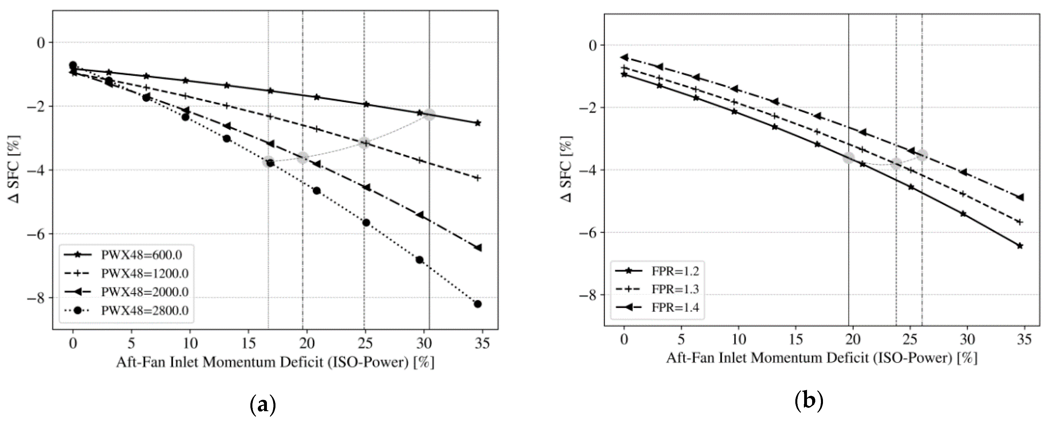
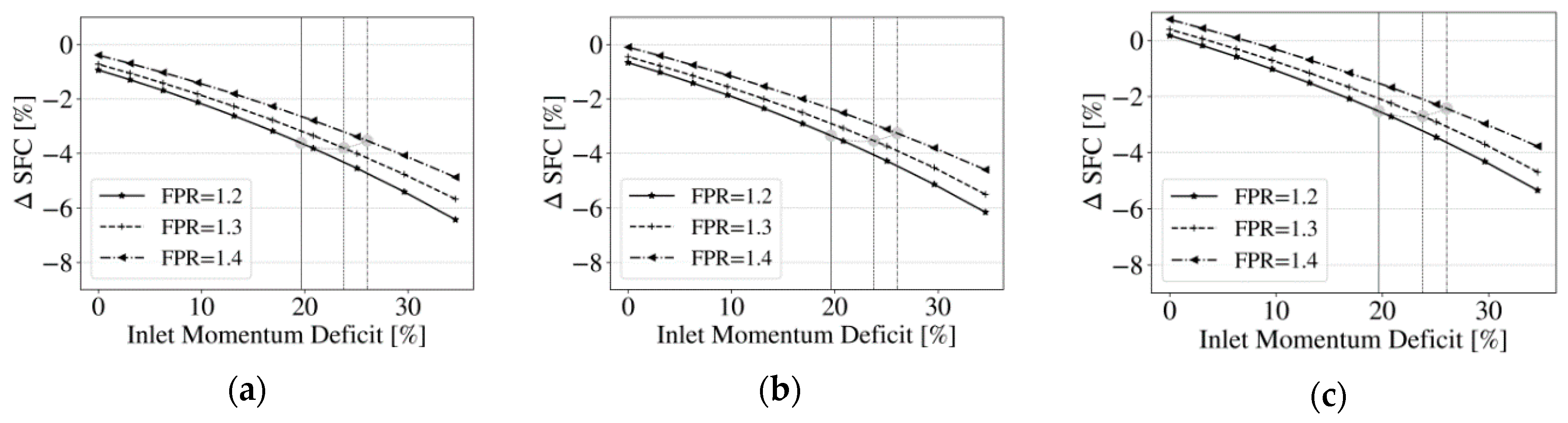
4.3.3. Inlet Momentum Deficit Sensitivity

The actual BLI benefit may have been underestimated since additional low momentum fluid may be captured into the aft-fan by taking advantage of fuselage diffusion and an optimized intake design; this may also lead to a flow redistribution radially with lower momentum fluid not directly being associated with a loss in total pressure [10]. In order to account for this uncertainty in accurately predicting the incoming momentum deficit, the following sensitivities were derived based on the results shown in Figure 8 by performing a linearization of the change in SFC at the achievable momentum deficit for each of the four cases considered:
[ Δ S F C Δ ( Δ I ) ] P W X = 2800   kW F P R = 1.2 0.20 ,
[ Δ S F C Δ ( Δ I ) ] P W X = 1200   kW   F P R = 1.2 0.10 ,
[ Δ S F C Δ ( Δ I ) ] P W X = 2000   kW   F P R = 1.3 [ Δ S F C Δ ( Δ I ) ] P W X = 2000   kW   F P R = 1.4 0.15 ,
It is interesting to notice that those sensitivities are almost not dependent on the aft-fan FPR, and they increase as the power setting rises. The given sensitivities may be applied directly to propagate a given variation (here ±25% as an example) in the incoming momentum deficit (e.g., due to the rather high uncertainty in quantifying this using flat plate theory), which, by using Equations (23)–(25) would translate into an SFC-variation for the four different cases as given in Table 5:
This again may be translated into a change in block fuel ΔBF using the given exchange rates from Table 4. Once more detailed information regarding the incoming momentum deficit is available (e.g., from detailed CFD studies as carried out in References [29,40]), the given sensitivities may be used to more reliably quantify the overall BF savings potential at the system level.

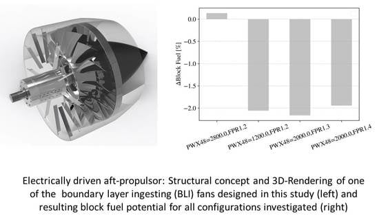
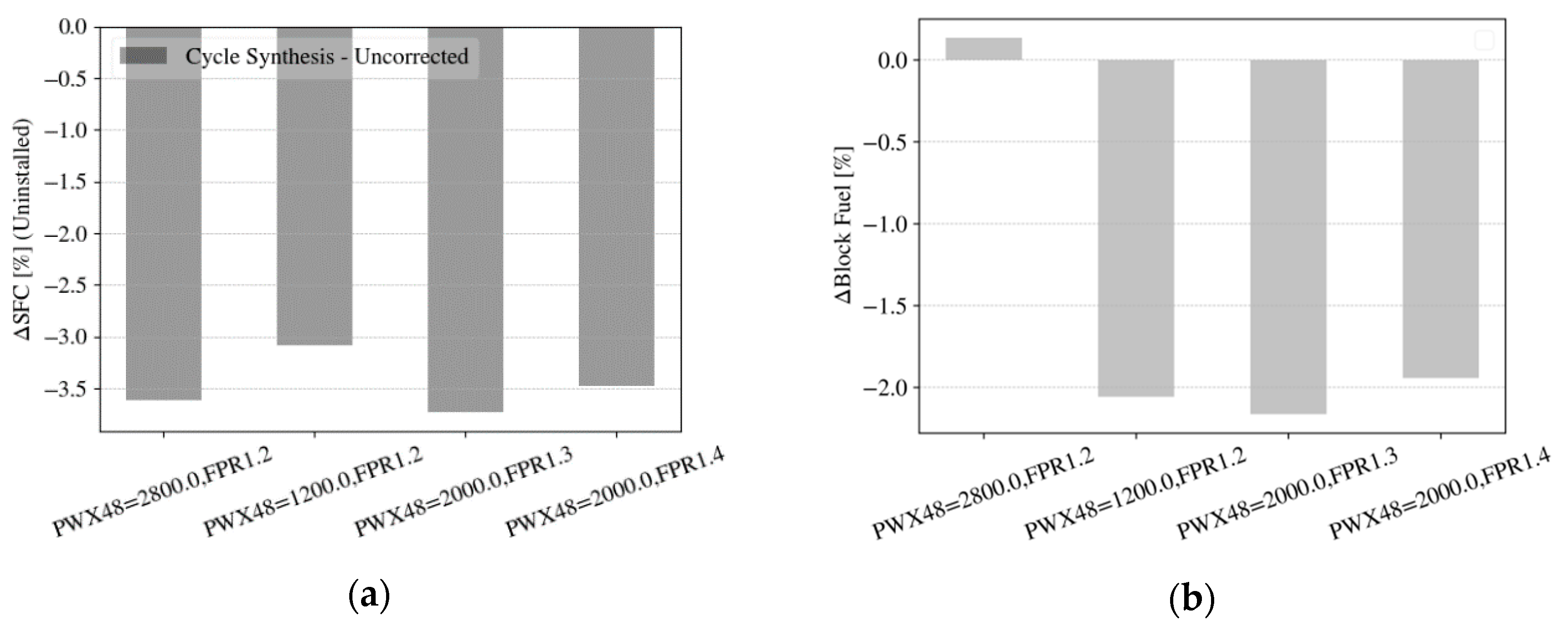
4.3.4. Block-Fuel Estimation of Selected Configurations

After applying all corrections and exchange rates as given in Table 4, a comparison between the uninstalled SFC benefits, as well as the mission-based block fuel savings is provided in Figure 32. One of the most striking observation is that for the high-power and low-FPR case (PWX48 = 2800 kW and FPR = 1.2) there is no remaining fuel burn benefit despite an equal level of uninstalled SFC benefit as compared to the other configurations. This is associated with the large weight of both, the aft-propulsor itself and, even more importantly, the electrical system. Moreover, the ranking of the other configurations has changed, slightly degrading the high-FPR case with FPR = 1.4, which was driven by lower achievable fan efficiency levels. The resulting mission fuel burn-saving for the best of the four configurations (PWX48 = 2000 kW and FPR = 1.3) is 2.2%. This estimate is considered very optimistic because a number of detrimental effects (e.g., re-configuration of the aircraft’s empennage with a T-tail, additional intake losses, boundary layer turbulence further impacting the BLI fan’s performance, etc.) have not been considered in this study and some assumptions made were rather optimistic (e.g., efficiency levels of the electrical system).

5. Summary and Conclusions

The main findings of this study shall be summarized again hereafter, in particular in the light of the research questions as posed at the beginning of this article. Regarding the sensitivity of the systems top-level parameters and the optimal choice thereof, the following conclusions were drawn:
  • Firstly, a sensitivity study was carried out in order to account for the uncertainty in predicting the incoming momentum deficit as induced by the fuselage boundary layer. Those sensitivities were quantified, allowing for a correction of the results if more detailed knowledge of the actual flow characteristics is available.
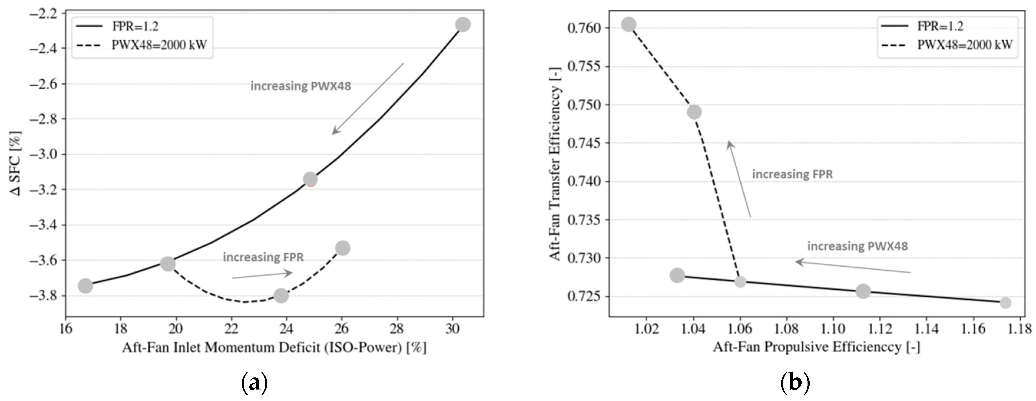
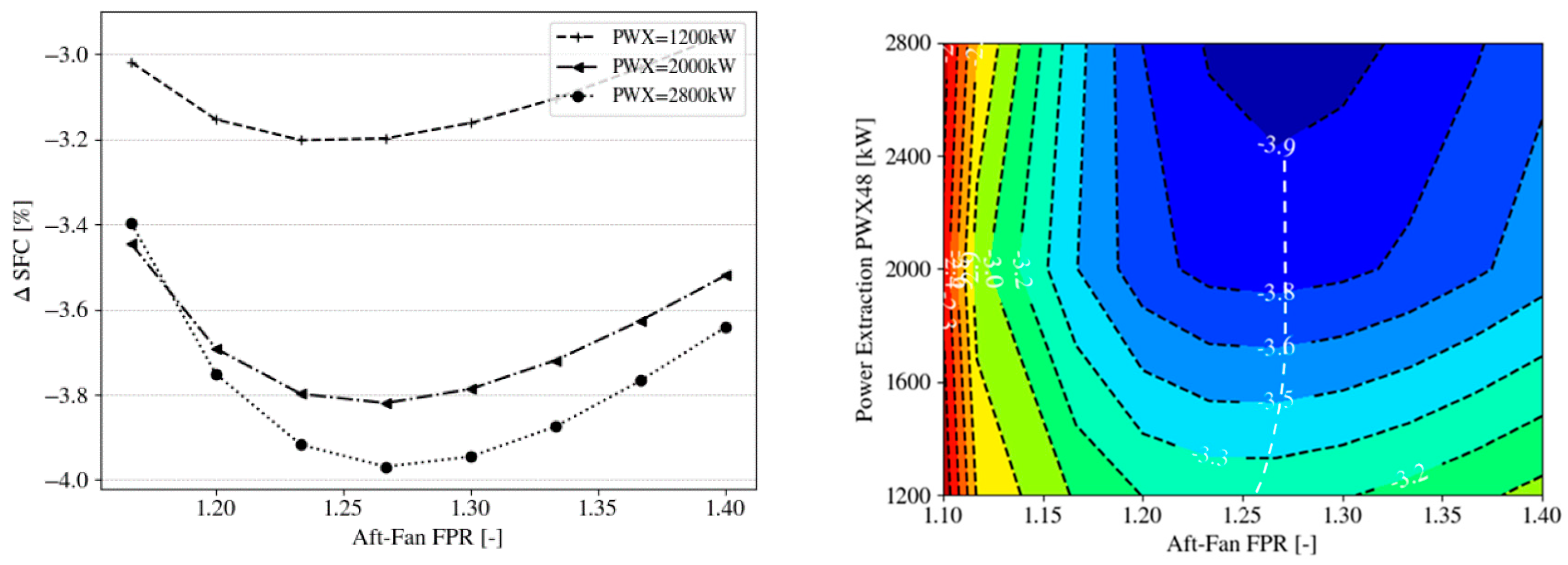
  • The optimal fan pressure ratio and power off-take were determined for a minimal uninstalled SFC benefit based on results from multi-point cycle synthesis. The results suggest that an optimal value of approximately FPR ≈ 1.27 for the aft-fan leads to an uninstalled SFC benefit of 3.9%, however, the ranges in SFC between the identified possible values of momentum deficit are on the same order as the total savings. In this context, the special role of transfer and propulsive efficiency was analyzed and discussed. At a certain level of PWX48, no further reduction in SFC was observed, due to a diminishing BLI effect and opposite trends in transfer efficiency levels between the main engine and the aft-fan. The main engine essentially traded propulsive efficiency for transfer efficiency and the benefit at the system level came from the aft-propulsor’s gain in propulsive efficiency at sufficient levels of power extraction. Further studies might involve a different strategy for designing the main engine by retaining the fan pressure ratio and allowing for a reduction in engine diameter and bypass ratio (as discussed in Reference [10]).
  • It was also discussed how this optimal SFC was translated to mission fuel burn based on derived exchange rates and how it was compromised by a number of factors, such as additional weight and drag. This also changed the ranking of the selected configurations, substantially penalizing larger power-off takes and smaller aft-fan FPR.
  • The average achievable benefit in terms of block fuel for the given configuration was estimated to be up to 2.2% compared with the baseline scenario under the given (optimistic) assumptions.
Furthermore, the choices of top-level parameters imposed the following implications on the conceptual design of the aft-fan:
  • Under the given assumptions, the fan rotor hub-to-tip ratio varies with increasing fan diameter and power off-take, which requires a dedicated design effort for given top-level parameters.
  • The impact of BLI on fan stage performance was firstly assessed by following a conventional design approach and then by applying the incoming boundary layer. This was done for four downselected cases based on conceptual design studies involving a streamline-curvature method.
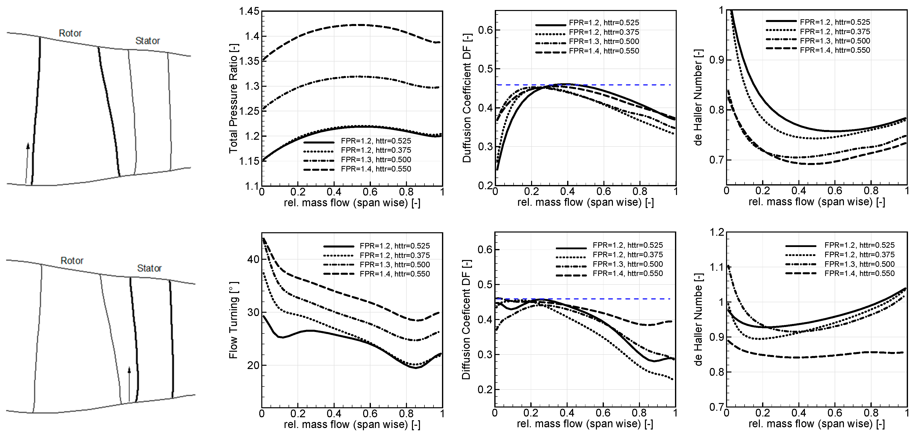
  • The baseline results suggest that the hub sections are likely to fail under the influence of the BLI, due to the massively increase turning requirements to meet an imposed fan pressure ratio distribution.
  • Several rotor design strategies were investigated to mitigate the effect of the BLI and allow for the design of an operational fan. In that context, the role of rotor tip speed was discussed, suggesting that higher Ψ-values be beneficial in terms of maintaining efficiency levels. This needs further confirmation with CFD-based design optimization studies. Furthermore, an increase in the total pressure ratio near the hub, leading to a quasi free-vortex design, was discussed and seemed beneficial in order to balance the flow radially. Further increasing the total pressure ratio to realize a descending pressure ratio profile was not investigated, but might help to homogenize the OGV outflow. This would require a higher value of the hub radius or respective hub-to-tip ratio in order to accommodate the high flow turning requirements at given tip speed.
  • Further design updates of the fan stage were realized by introducing local contraction by an increased hub line curvature and associated pressure gradient in order to unload the rotor and the OGV and hence, limit DF values for a given low turning under BLI.
  • Based on the results, it is believed that high levels of efficiency can be retained, at least for the given axisymmetric pressure profile. Off-design performance, however, needs to be further addressed, in particular considering the location of the Take-Off point at constant power extraction levels, which was located close to the stability limit for almost all designs. This either promotes the use of variability, or the decision to go for higher levels of aft-fan FPR.

Author Contributions

“Manuscript editing”: All, “Engine performance modelling”: X.Z., “Map processing and integration into performance model”: M.K., “Electrical System Dimensioning”: S.S., “Literature Survey and Boundary Layer Considerations”: E.R., “Fan conceptual design tool and software programming”: M.S., “Conceptualization, guidance and technical input, internal funding acquisition”: K.K., “Conceptualization, fan design and BLI assessment strategy, writing and draft manuscript preparation, internal funding acquisition”: R.S.

Funding

This research received no external funding.

Conflicts of Interest

The authors declare no conflict of interest. However, several activities investigating a similar configuration, currently receiving external funding are ongoing in both organizations. In this context, it needs to be stressed that all results in this paper, including their analysis, data processing and way of visualization, as well as dedicated designs, were, if not indicated otherwise, exclusively based on data from open literature or derived in the context of this joint bi-lateral effort between German Aerospace Center (DLR) and Mälardalen University (MDH), with no direct link to other ongoing studies whatsoever.

Abbreviations

A/CAircraft
ACDCAdvanced Compressor Design Code (Streamline Curvature Method as used in this study)
ACAREAdvisory Council for Aeronautical Research in Europe
AFAft-Fan
BLIBoundary Layer Ingesting
BFBlock Fuel
CFDComputational Fluid Dynamics
CeRASCentral Reference Aircraft Data System
CPACSCommon Parametric Aircraft Configuration Schema
DLRDeutsches Zentrum fuer Luft- und Raumfahrt/German Aerospace Center
EVAEnVironmental Assessment Framework
FPRFan (total) pressure ratio
GTGas Turbine (=Main Engine)
IGVInlet Guide Vane
LEBlade Row Leading Edge
LPC/HPCLow/High-Pressure Compressor
LPT/HPTLow/High-Pressure Turbine
MEMain Engine
MDHMälardalen Högskola
OGVOutlet Guide Vane
OPROverall Pressure Ratio
PIDController with Proportional, Integral and Differential Terms
SLCStreamline-Curvature Method (also referred to as Throughflow-Method). The method applied here is ACDC (DLR in-house code).
STARC-ABLSingle-aisle Turboelectric Aircraft with an Aft Boundary Layer Propulsor
TOCTop-of-Climb
TEBlade Row Trailing Edge

Nomenclature and Performance Metrics Definition

cu2,meanVelocity[m/s]Mean circumferential velocity at rotor outlet. Mean here meaning at a radial position dividing the total mass flow in half.Definition according to Reference [25]
ΔIMomentum Deficit (Intergal)[%]Aft-fan incoming momentum deficit with respect to ram momentum at given fligh speed v0[v0,BLI * w92,BLI v0 * w92]/(v0 * w92)
de-Haller[-]Blade row flow acceleration/diffusion: Velocity ratio at blade row outlet over inlet in relative system
DDiameter[m](Fan) outer diameter
DFDiffusion coefficient[-]Rotor or OGV blade loading resulting from flow diffusion and flow turningDefinition according to Lieblein as, e.g., in References [24] or [25]
EcoreEnergy per time unit[W]Core exit potential power; the core exit is where the fan core and LPC power requirements are satisfied in the LPT expansion
Ep,coreEnergy potential per time unit[W]Power available after all power requirements of the core compression processes (including power off-take) are satisfied
EfuelEnergy per time unit[W]Power as introduced by the fuelEfuel = wf × FHV
ΔEkin,jetsEnergy per time unit[W]Change in jet kinetic power
FNNet Thrust[N]Engine net thrust
FHVFuel heat value[J/kg]
ΔhtEnthalpy[J/kg]Enthalpy change over the fan stage
MaMach number[-]
MaffFan-face Mach Number[-](Meridional or axial) Mach number at fan entry
N48Rotational Speed[1/min]Aft-fan rotational speed
p0Total pressure[Pa]Average Inlet Total Pressure
P13Q2Main engine fan total pressure ratio[-]Bypass section of the fan
P23Q2Main engine fan total pressure ratio[-]Core section of the fan
PRnPressure ratio split[-](Logarithmic) Pressure ratio split between LPC and HPCDefinition as in Reference [6]
PWX48Power Extraction[kW]Power input to the aft-fanPWX48 = PWX46 * ηmech * ηel
PWX46Power Extraction[kW]PWX46 extraction from the LP shaft
RPMRotational speed[1/min]
Re [-]Reynolds Number
rRadius[m]
SFNSpecific Thrust[m/s]
SFCSpecific Fuel Consumption[g/(kN*s)]
TtTotal Temperature[K]Total Temperature at component inlet 1 or outlet 2
utip(,c)Circumferential velocity[m/s]Rotor blade (corrected) tip speed
v0Velocity[m/s]Flight velocity
v0,BLIVelocity[m/s]Velocity at fan entry due to BLI
vid,95Velocity[m/s]Aft-fan nozzle exit velocity (ideally expanded)
vid,18Velocity[m/s]Main engine bypass nozzle exit velocity (ideally expanded)
v18Velocity[m/s]Mixed out jet velocity comprising of the cold jet in the main engine bypass and the hot jet after the core nozzle
vid,7Velocity[m/s]Main engine core nozzle exit velocity (ideally expanded)
VcoldQhotJet Velocity Ratio[-]Ratio of the velocity of cold (bypass) jet over the core nozzle velocity
w18Mass flow rate[kg/s]Mass flow through the fan bypass
w2Mass flow rate[kg/s]Engine inlet mass flow
w92Mass flow rate[kg/s]Aft-fan mass flow rate
w7Mass flow rate[kg/s]Core mass flow rate
wfMass flow rate[kg/s]Fuel mass flow rate flow
ηelEfficiency[%]Transfer efficiency of the electrical system
ηmechEfficiency[%]Efficiency of the mechanical system (e.g., bearing losses etc.)
ηthThermal Efficiency[%]Increase of the kinetic energy of the gas stream over the amount of heat employedηth = ηcore * ηtrans
ηcoreCore Efficiency[%]Ratio of energy available after all the power requirements of the core compression processes are satisfied and the fuel energyDefinitions for the main engine, aft-fan and system according to Equations (4) and (9)
ηtransTransmission Efficiency[%]Quality of the energy transfer from the core stream to the bypass streamDefinitions for the main engine, aft-fan and system according to Equations (5) and (7), (11) and (15)
ηpropPropulsive Efficiency[%]Useful propulsive energy over the kinetic energy loss of the jetDefinitions for the main engine, aft-fan and system according to Equations (6), (8), (10) and (14)
ηovOverall Efficiency[%]Resulting propulsive power to the energy content of the fuelDefinitions for the main engine, aft-fan and system according to Equation (17)
ηisIsentropic Efficiency[%]Component isentropic efficiency η i s = [ π t γ 1 γ 1 ] [ T t 2 / T t 1 1 ]
ηpolPolytropic Efficiency[%]Component polytropic efficiency
νHub-to-tip ratio[-]Rotor leading edge hub to tip radius
π t Total Pressure Ratio[-]Fan stage total pressure ratio
ΨFan Rotor Work Coefficient[-] Ψ = Δ h t u m e a n 2 c u , 2 , m e a n u m e a n
More details, e.g., in References [24] or [25]

Appendix A

Table A1. Assumptions (top) and parameters (bottom) for the reference gas generator/main engine [6].
EIS 2035 AssumptionsUnitValue
Gear Box Speed Ratio-3.0
Fan bypass/core polytropic efficiency-0.946/0.956
Low pressure compressor polytropic efficiency-0.923
High pressure compressor polytropic efficiency-0.925
High pressure turbine polytropic efficiency-0.897
Low pressure turbine polytropic efficiency-0.929
Combustor Outlet Ttemperature @ hot day TOC (ISA + 10 K)K1900
Turbine metal temperature @ hot day T/O (ISA + 15 K)K1240
Baseline ParametersUnitValue
Cruise Specific Thrust SFNm/s91
Cruise OPR-55
Cruise VcoldQhot-0.77 1
Cruise PRn-0.402
TOC Bypass Ratio BPR-15.2
TOC Fan Pressure Ratio FPR-1.48
TOC LPC Pressure Ratio-3.68
TOC HPC Pressure Ratio-12.32
TOC HPC Exit TemperatureK979
HPT Cooling flow fraction%21.2
LPT Cooling flow fraction%1.1
1 The given value is the mission-based optimum. In this paper, a value of 0.9 will be used, which is expected to be close to the block fuel optimum as explained in the text.
Table A2. Main engine gas turbine and BLI propulsor matching scheme.
Key Engine ParametersUnitsHot-Day Top-of-Climb Conditions (ISA+10, FL350, Mach 0.78)Hot-Day End-of-Runway Take-Off Conditions (ISA+15, FL0, Mach 0.25)Cruise Conditions (ISA, FL350, Mach 0.78)
Specific thrustm/sSolved for in the analysisSolved for in the analysisSolved for in the analysis
Jet velocity ratio-Solved for in the analysisSolved for in the analysisSynthesis Target 2
Pressure ratio split exponent-Solved for in the analysisSolved for in the analysisSynthesis Target 3
Fan tip over hub pressure rise ratio-TargetSolved for in the analysisSolved for in the analysis
Overall pressure ratio-Solved for in the analysisSolved for in the analysisSynthesis Target 4
HPC outlet temperatureKSolved for in the analysisSolved for in the analysisSolved for in the analysis
HPT 1st vane metal temperatureKSolved for in the analysisSynthesis Target 5Solved for in the analysis
HPT 1st rotor metal temperatureKSolved for in the analysisSynthesis Target 6Solved for in the analysis
HPT 2nd vane metal temperatureKSolved for in the analysisSynthesis Target 7Solved for in the analysis
HPT 2nd rotor metal temperatureKSolved for in the analysisSynthesis Target 8Solved for in the analysis
LPT 1st vane metal temperatureKSolved for in the analysisSynthesis Target 9Solved for in the analysis
LPT 1st rotor metal temperatureKSolved for in the analysisSynthesis Target 10Solved for in the analysis
BLI Fan shaft powerkWTargetTarget/Solved for in the analysisTarget/Solved for in the analysis
ThrustkNTargetTargetTarget
BLI Fan pressure ratio-FixedSolved for in the analysisSolved for in the analysis
BLI Fan inlet mass flowkg/sVariableSolved for in the analysis †Solved for in the analysis †
Engine inlet mass flowkg/sFixedSolved for in the analysisSolved for in the analysis
Fan tip pressure ratio-Synthesis Variable 1Solved for in the analysisSolved for in the analysis †
Bypass ratio-Synthesis Variable 2Solved for in the analysisSolved for in the analysis †
Fan root pressure ratio-VariableSolved for in the analysisSolved for in the analysis
LPC pressure ratio-Synthesis Variable 3Solved for in the analysisSolved for in the analysis †
HPC pressure ratio-Synthesis Variable 4Solved for in the analysisSolved for in the analysis †
HPT 1st stage vane cooling flow (% HPC flow)%Synthesis Variable 5same as @ToC †same as @ToC
HPT 1st stage rotor cooling flow (% HPC flow)%Synthesis Variable 6same as @ToC †same as @ToC
HPT 2nd stage vane cooling flow (% HPC flow)%Synthesis Variable 7same as @ToC †same as @ToC
HPT 2nd stage rotor cooling flow (% HPC flow)%Synthesis Variable 8same as @ToC †same as @ToC
HPT 2nd stage cooling flow extraction point%Fixedsame as @ToCsame as @ToC
LPT 1st stage vane cooling flow (% HPC flow)%Synthesis Variable 9same as @ToC †same as @ToC
LPT 1st stage rotor cooling flow (% HPC flow)%Synthesis Variable 10same as @ToC †same as @ToC
LPT cooling flow extraction point%Fixedsame as @ToCsame as @ToC
Combustor outlet temperatureKVariableVariableSynthesis Target 1
Core nozzle aream2Solved for in the analysisSolved for in the analysisSolved for in the analysis
Bypass nozzle aream2Solved for in the analysisSolved for in the analysisSolved for in the analysis
Core inlet mass flowkg/sSolved for in the analysisSolved for in the analysisSolved for in the analysis
High pressure turbine rotor inlet temperatureKSolved for in the analysisSolved for in the analysisSolved for in the analysis
Turbomachines polytropic efficiency%FixedSolved for in the analysisSolved for in the analysis
Engine intake pressure loss dP/P%FixedSolved for in the analysisSolved for in the analysis
Combustor pressure loss dP/P%FixedSolved for in the analysisSolved for in the analysis
Ducts pressure loss dP/P%FixedSolved for in the analysisSolved for in the analysis
Nozzles thrust coefficient%FixedSolved for in the analysisSolved for in the analysis
Shafts mechanical efficiency%FixedSolved for in the analysisSolved for in the analysis
Gearbox speed ratio%Fixedsame as @ToCsame as @ToC
Gearbox mechanical efficiency%FixedSolved for in the analysisSolved for in the analysis
† Varied using corresponding synthesis variable at top-of-climb condition.
Table A3. Performance parameter and weight estimation in electrical components for the different cases considered (Pess. = pessimistic, Opt. = optimistic assumptions; numbers in bold highlight the power off-takes for the cases considered in this study and described in Section 4.2).
ComponentEfficiencySpecific PowerCase 1Case 2Case 3
[%][kW/kg]PowerLossWeightPowerLossWeightPowerLossWeight
*[A/(kg/m)][kW] [kg][kW] [kg][kW] [kg]
Pess.Opt. Pess.Opt. Pess.Opt. Pess.Opt.
Motor196.0131612004892752800112215175200080154125
Inverter199.0101912501312566291729292154208321208110
Circ. Protection499.520020063113131314732929291052212121
Cable299.6170*170*634529029014801267767710578484484
Rectifier299.010196371312767148630297156106221212112
Generator296.013166435199801501120231188107286165134
Thermal System 0.681.6 20286 4712001117 337143
Total System 137948677 32022131579 22915811128

References

  1. International Cival Aviation Organization: On Board a Sustainable Future, ICAO Environmental Report. Available online: https://www.icao.int/environmental-protection/Pages/env2016.aspx (accessed on 13 October 2019).
  2. ACARE Strategic Research & Innovation Agenda. Advisory Council for Aviation Research and Innovation in Europe, 2017; Volume 1. Available online: https://www.acare4europe.org/sites/acare4europe.org/files/document/ACARE-Strategic-Research-Innovation-Volume-1.pdf (accessed on 13 October 2019).
  3. Lents, C.E.; Hard, L.; Rheaume, J.; Kohlman, L. Parallel Hybrid Gas-Electric Geared Turbofan Engine Conceptual Design and Benefits Analysis. In Proceedings of the 52nd AIAA/SAE/ASEE Joint Propulsion Conference, Salt Lake City, UT, USA, 25–27 July 2016. [Google Scholar]
  4. Freeh, J.E.; Steffen, C.J.; Larosiliere, L.M. Off-design performance analysis of a solid-oxide fuel cell/gas turbine hybrid for auxiliary aerospace power. In Proceedings of the ASME 2005 3rd International Conference on Fuel Cell Science, Engineering and Technology, Ypsilanti, MI, USA, 23–25 May 2005. [Google Scholar]
  5. Lupelli, L.; Geis, T. A Study on the Integration of the IP Power Offtake System within the Trent 1000 Turbofan Engine. Available online: https://core.ac.uk/reader/14703878 (accessed on 13 October 2019).
  6. Zhao, X.; Sahoo, S.; Kyprianidis, K.; Rantzer, J.; Sielemann, M. Off-design performance analysis of hybridised aircraft gas turbine. Aeronaut. J. 2019, 123, 1999–2018. [Google Scholar] [CrossRef]
  7. Smith, A.M.O.; Roberts, H.E. The Jet Airplane Utilizing Boundary Layer Ingestion for Propulsion. J. Aeronaut. Sci. 1947, 14, 97–109. [Google Scholar] [CrossRef]
  8. Smith, L.H. Wake Ingesting Propulsion Benefit. J. Propuls. Power 1993, 9, 74–82. [Google Scholar] [CrossRef]
  9. Plas, A.P.; Sargeant, M.A.; Madani, V.; Chrichton, D.; Greitzer, E.M.; Hynes, T.P.; Hall, C.A. Performance of a Boundary Layer Ingesting (BLI) Propulsion System. In Proceedings of the 45th AIAA Aerospace Sciences Meeting and Exhibit, Reno, NV, USA, 8–11 January 2007. AIAA 2007-450. [Google Scholar]
  10. Welstead, J.R.; Felder, J.L. Conceptual Design of a Single-Aisle Turboelectric Commercial Transport with Fuselage Boundary Layer Ingestion. In Proceedings of the 54th AIAA Aerospace Sciences Meeting/Conference, San Diego, CA, USA, 4–8 January 2016. [Google Scholar] [CrossRef] [Green Version]
  11. Yildirim, A.; Gray, J.S.; Mader, C.A.; Martins, J. Aeropropulsive Design Optimization of a Boundary Layer Ingestion System. In Proceedings of the AIAA Aviation 2019 Forum, Dallas, TX, USA, 17–21 June 2019. [Google Scholar]
  12. Gray, J.S.; Kenway, G.K.; Mader, C.A.; Martins, J. Aero-propulsive Design Optimization of a Turboelectric Boundary Layer Ingestion Propulsion System. In Proceedings of the 2018 Aviation Technology, Integration, and Operations Conference, Atlanta, GA, USA, 25–29 June 2018. [Google Scholar]
  13. Kenway, G.K.; Kiris, C.C. Aerodynamic Shape Optimization of the STARC-ABL Concept for Minimal Inlet Distortion. In Proceedings of the 2018 AIAA/ASCE/AHS/ASC Structures, Structural Dynamics, and Materials Conference, Kissimmee, FL, USA, 8–12 January 2018. [Google Scholar]
  14. Seitz, A.; Isikveren, A.T.; Hornung, M. Pre-concept performance investigation of electrically powered aero-propulsion systems. In Proceedings of the 49th AIAA/ASME/SAE/ASEE Joint Propulsion Conference, San Jose, CA, USA, 14–17 July 2013; p. 3608. [Google Scholar]
  15. Isikveren, A.T.; Pornet, C.; Vratny, P.C.; Schmidt, M. Conceptual studies of future hybrid-electric regional aircraft. In Proceedings of the 22nd International Symposium on Air Breathing Engines, Phoenix, AZ, USA, 22–25 October 2015. [Google Scholar]
  16. CeRAS Central Reference Aircraft Data System. Available online: https://ceras.ilr.rwth-aachen.de/ (accessed on 13 December 2019).
  17. Kyprianidis, K.G.; Quintero, R.F.C.; Pascovici, D.S.; Ogaji, S.O.T.; Pilidis, P.; Kalfas, A.I. EVA: A Tool for EnVironmental Assessment of Novel Propulsion Cycles. In Proceedings of the ASME Turbo Expo: Power for Land, Sea, and Air, Berlin, Germany, 9–13 June 2008; pp. 547–556. [Google Scholar]
  18. Schlichting, H. Boundary Layer Theory (Grenzschicht-Theorie); Springer: Karlsruhe, Germany, 1964. [Google Scholar]
  19. Klabes, A.; Appely, C.; Herr, M. Fuselage Excitation During Cruise Flight Conditions: Measurement and Prediction of Pressure Point Spectra. In Proceedings of the 21st AIAA/CEAS Aeroacoustics Conference, Dallas, TX, USA, 22–26 June 2015. AIAA Paper 2015-3115. [Google Scholar]
  20. Schnös, M.; Nicke, E. Exploring a Database of Optimal Airfoils for Axial Compressor Design. In Proceedings of the 23rd International Symposium on Air Breathing Engines, Manchester, UK, 3–8 September 2017. ISABE Paper 2017-21493. [Google Scholar]
  21. Schnös, M.; Voß, C.; Nicke, E. Design Optimization of a Multi-Stage Axial Compressor Using Throughflow and a Database of Optimal Airfoils. In Proceedings of the GPPS Montreal 18 Conference, Montreal, QC, Canada, 7–9 May 2018. [Google Scholar]
  22. Kavvalos, M.; Zhao, X.; Schnell, R.; Aslanidou, I.; Kalfas, A.; Kyprianidis, K. A Modelling Approach of Variable Geometry for Low Pressure Ratio Fans. In Proceedings of the International Society of Air Breathing Engines, Canberra, Australia, 23–27 September 2019. ISABE Paper 2019-24382. [Google Scholar]
  23. Kyprianidis, K.G. Future Aero Engine Designs: An Evolving Vision. In Advances in Gas Turbine Technology; Benini, E., Ed.; IntechOpen: London, UK; Available online: https://www.intechopen.com/books/advances-in-gas-turbine-technology/future-aero-engine-designs-an-evolving-vision (accessed on 4 November 2011). [CrossRef] [Green Version]
  24. Schnell, R.; Goldhahn, E.; Julain, M. Design and Performance of a Low Fan-Pressure-Ratio Propulsion System. In Proceedings of the International Society of Air Breathing Engines, Canberra, Australia, 23–27 September 2019. ISABE Paper 2019-24017. [Google Scholar]
  25. Crichton, D.; Xu, L.; Hall, C.A. Preliminary Fan Design for a Silent Aircraft. J. Turbomach. 2017, 129, 184–191. [Google Scholar] [CrossRef]
  26. Kurzke, J. Preliminary Engine Design. In Aero Engine Design: From State of the Art Turbofans Towards Innovative Architectures; Lecture Series 2008-03; Von Karman Institute (VKI): Brussels, Belgium, 2008. [Google Scholar]
  27. Cumpsty, N.A. Compressor Aerodynamics; Krieger Publishing Company: Malabar, FL, USA, 2004. [Google Scholar]
  28. Grieb, H. Verdichter Für Turbo-Flugtriebwerke/Aero Engine Compressors; Springer: Berlin/Heidelberg, Germany, 2009; ISBN 978-3-540-34374-5. [Google Scholar]
  29. Lee, B.J.; Liou, M.F. Aerodynamic Design and Optimization of Fan Stage for Boundary Layer Ingestion Propulsion System. In Proceedings of the 10th International Conference on Computational Fluid Dynamics (ICCFD10), Barcelona, Spain, 9–13 July 2018. ICCFD10-091. [Google Scholar]
  30. Mennicken, M.; Schönweitz, D.; Schnoes, M.; Schnell, R. Conceptual Fan Design for Boundary Layer Ingestion. In Proceedings of the ASME Turbo Expo 2019: Turbomachinery Technical Conference and Exposition, Phoenix, AZ, USA, 17–21 June 2019. ASME Paper GT2019-90257. [Google Scholar]
  31. Dever, T.P. Assessment of Technologies for Noncryogenic Electric Propulsion; Report NASA/TP—2015-216588; NASA: Cleveland, OH, USA, 2015.
  32. Duffy, K.P. Electric Motors for Non-Cryogenic Hybrid Electric Propulsion. In Proceedings of the 51st AIAA/SAE/ASEE Joint Prpulsion Conference, Orlando, FL, USA, 27–29 July 2015. [Google Scholar]
  33. Jansen, R.; Bowman, C.; Jankovysky, A.; Dyson, R.; Felder, J. Overview of NASA Electrified Aircraft Prpulsion (EAP) Research for Large Subsonic Transports. In Proceedings of the 53rd AIAA/SAE/ASEE Joint Propulsion Conference, Atlanta, GA, USA, 10–12 July 2017. [Google Scholar]
  34. National Academies of Sciences and Medicine. Commercial Aircraft Propulsion and Energy Systems Research: Reducing Global Carbon Emission; National Academies Press: Washington, DC, USA, 2016. [Google Scholar]
  35. Lee, B.J.; Liou, M.-F. Aerodynamic Conceptual Design of Boundary Layer Ingestion Propulsor Systems: A Quasi-2d Through Flow Analysis Method and Multi-Fidelity Propulsor Design Framework. In Proceedings of the ASME Turbo Expo 2018: Turbomachinery Technical Conference and Exposition, Lillestrom (Oslo), Norway, 11–25 June 2018. ASME Paper GT2018-75861. [Google Scholar]
  36. Sahoo, S.; Zhao, X.; Kyprianidis, K. Performance Assessment of an Integrated Parallel Hybrid-Electric Propulsion System Architecture. In Proceedings of the ASME Turbo Expo 2019: Turbomachinery Technical Conference and Exposition, Phoenix, AZ, USA, 17–21 June 2019. ASME Paper GT2019-91459. [Google Scholar]
  37. Lengyel-Kampmann, T.; Voß, C.; Nicke, E.; Rud, K.-P.; Schaber, R. Generalized Optimization of Counter-Rotating and Single-Rotating Fans. In Proceedings of the ASME Turbo Expo, Duesseldorf, Germany, 16–20 June 2014. ASME Paper 2014-26008. [Google Scholar]
  38. Kyprianidis, K.; Rolt, A.M. On the Optimization of a Geared Fan Intercooled Core Engine Design. J. Eng. Gas Turbines Power 2015, 137, 041201. [Google Scholar] [CrossRef]
  39. Jenkinson, L.; Simkin, P.; Rhodes, D. Civil Jet Aircraft Design; Arnold: London, UK, 1999; ISBN 0-340-74152-X. [Google Scholar]
  40. Gray, S.; Mader, C.A.; Kenway, G.K.W.; Martins, J.R.R.A. Modeling Boundary Layer Ingestion Using a Coupled Aeropropulsive Analysis. J. Aircr. 2017, 55, 1191–1999. [Google Scholar] [CrossRef]
Figure 1. Turbo-electric aircraft concept with aft propulsion as investigated in the present study and initially introduced in Reference [10] (left), boundary layer ingestion (BLI)-propulsor located in the aft section of the aircraft resulting from the present study (center) and engine layout of the main under-wing engines and aft-fan (right).
Aerospace 06 00134 g001
Figure 2. Sketch of the A/C tail cone and derived geometric boundary conditions for the aft-fan conceptual design, as well as assumptions on the incoming boundary layer based on turbulent flat-plate boundary layer profiles.
Aerospace 06 00134 g002
Figure 3. Main engine gas turbine cycle and station definition.
Aerospace 06 00134 g003
Figure 4. Computational grid and station definition as input parameters to the streamline-curvature method ACDC (Advanced Compressor Design Code [20,21]) used for the aft-propulsor conceptual design.
Aerospace 06 00134 g004
Figure 5. Coupling procedure of the performance model (Environmental Assessment, EVA) with the streamline-curvature method (ACDC); Δηis is the difference between values of the current and the last iteration, ΔFPR the respective difference between current iteration and the target pressure ratio (FPR).
Aerospace 06 00134 g005
Figure 6. Location of the mission points in the aft-fan performance maps—Results using standard maps as initially available in the performance model (a) and updated characteristics from dedicated fan design efforts using the SLC-method for FPR = 1.2 and Ψ = 0.5 (b).
Aerospace 06 00134 g006
Figure 7. Location of the mission points as considered in this study in the aft-fan performance characteristics and their respective dependence on the choice of fan corrected tip speed or work coefficient Ψ, respectively—Results for FPR = 1.2/Ψ = 0.6 (a), FPR = 1.2/Ψ = 0.4 (b) and FPR = 1.3/Ψ = 0.5 (c).
Aerospace 06 00134 g007
Figure 8. Sensitivity of the specific fuel consumption (SFC, uninstalled) on incoming momentum deficit at different levels of power extraction PWX48 at constant fan pressure ratio FPR = 1.2 (a) and different aft-fan pressure ratio levels at PWX48 = 2000 kW (b)—The vertical lines denote the theoretically captured momentum deficit based on flat-plate assumptions; the light grey markers indicate the respective intersection with the PWX (a) or FPR (b) sensitivity lines and are considered achievable configurations.
Aerospace 06 00134 g008
Figure 9. Achievable configurations in terms of realistic momentum deficit and respective SFC benefit with varying FPR and PWX48 (a) and transfer efficiency vs. propulsive efficiency for the same configurations (b).
Aerospace 06 00134 g009
Figure 10. Uninstalled SFC benefit for all achievable configurations with varying aft-fan FPR (left) and power off-take PWX48 vs. aft-fan pressure ratio with contours color coding the relative SFC (right).
Aerospace 06 00134 g010
Figure 11. Contours of aft-fan transfer efficiency (a) and propulsive efficiency (b) as a function of power extraction PWX48 and fan pressure ratio FPR.
Aerospace 06 00134 g011
Figure 12. Contours of the main engine transfer efficiency (a) and propulsive efficiency (b) as a function of power extraction PWX48 and aft-fan pressure ratio FPR.
Aerospace 06 00134 g012
Figure 13. Contours of the system transfer efficiency (a) and propulsive efficiency (b) as a function of power extraction PWX48 and aft-fan pressure ratio FPR.
Aerospace 06 00134 g013
Figure 14. Contours of the product of transfer efficiency and propulsive efficiency as a function of power extraction PWX48 and aft-fan pressure ratio FPR for the aft-fan (a), the main engine (b) and the system (c).
Aerospace 06 00134 g014
Figure 15. Dependence of the specific fuel consumption (SFC, uninstalled) on the gas turbine jet velocity ratio for different scenarios (a) and jet velocity ratio of the main engine vs. system jet velocity ratio for the same selected cases (b).
Aerospace 06 00134 g015
Figure 16. Sensitivity of the specific fuel consumption (SFC, uninstalled) on incoming momentum deficit and fan pressure ratio FPR at constant PWX48 = 2000 kW for different gas turbine jet velocity ratios—Results for VcoldQhot = 0.9 (a), VcoldQhot = 0.8 (b) and VcoldQhot = 0.7 (c).
Aerospace 06 00134 g016
Figure 17. Main engine fan pressure ratio (a) and resulting thrust contribution from the aft-fan in relation to the overall thrust (b) for downselected cases at Cruise conditions. NB: The thrust ratio of the reference case is technically zero, and hence, not included in plot (b).
Aerospace 06 00134 g017
Figure 18. Gas generator core efficiency (a) as well as LPC and HPC component efficiencies (b) at cruise conditions for all downselected cases.
Aerospace 06 00134 g018
Figure 19. Aft-fan diameter (a) and hub-to-tip ratio, (b) dependence on incoming momentum deficit at different levels of power extraction PWX48 at constant fan pressure ratio FPR = 1.2.
Aerospace 06 00134 g019
Figure 20. Aft-fan diameter (a) and hub-to-tip ratio (b) dependence on incoming momentum deficit at different levels of aft-fan pressure ratio FPR at constant power extraction PWX48 = 2000 kW.
Aerospace 06 00134 g020
Figure 21. Aft-fan configurations resulting from downselection and considered for conceptual design of the aft-fan (right), and respective incoming boundary layer profiles (left).
Aerospace 06 00134 g021
Figure 22. Span-wise (as per mass flow fraction) distribution of major fan performance parameters resulting from conceptual design (non-BLI, baseline cases)—Results for the rotor (top row) and the OGV (bottom row).
Aerospace 06 00134 g022
Figure 23. Effect of the incoming boundary layer on the span-wise distribution of the meridional Mach number Mmer—Results for the baseline scenario (non-BLI, top row) and with inlet boundary layer profile applied (bottom row).
Aerospace 06 00134 g023
Figure 24. Corrected tip-speed or respective Ψ-sensitivity of the baseline design regarding an incoming boundary layer (results shown for FPR = 1.2, PWX48 = 2000 kW).
Aerospace 06 00134 g024
Figure 25. Span-wise (as per mass flow fraction) distribution of major fan performance parameters resulting from conceptual design (non-BLI baseline, BLI effect on baseline and updated design to account for the BLI effect)—Results for the rotor (top row) and the OGV (bottom row); dashed blue lines represent DF design target/limit.
Aerospace 06 00134 g025
Figure 26. Geometric changes made to accommodate the BLI effect—Example for FPR = 1.2 and Ψ = 0.5 baseline case (solid lines) and BLI design updated (Q-FV, as shown in Figure 25, dashed lines). Results of inlet flow angle, geometric angle and axial chord for the rotor (a, b and c, respectively) and for the OGV (d, e and f, respectively)
Aerospace 06 00134 g026
Figure 27. 3D blade shapes of the baseline geometry (grey) and updated BLI design (green) with restaggered blade and additional hub contraction in both rotor and OGV region.
Aerospace 06 00134 g027
Figure 28. Structural concept and 3D rendering of the resulting aft-propulsor design for FPR = 1.3.
Aerospace 06 00134 g028
Figure 29. Span-wise (as per mass flow fraction) distribution of major fan performance parameters resulting from conceptual design (non-BLI baseline, BLI design update and redesign with IGV)—Results for the rotor (top row) and the OGV (bottom row) for FPR = 1.2 and Ψ = 0.5.
Aerospace 06 00134 g029
Figure 30. Schematic of the electrical drivetrain.
Aerospace 06 00134 g030
Figure 31. Aft-propulsor and electrical system weight t based on data taken from Reference [10] (NASA) and data as described in the previous Section 4.3.1 yielding different technology levels (a) and additional aft-propulsor profile drag contribution in relation to total aircraft drag (b).
Aerospace 06 00134 g031
Figure 32. Relative specific fuel burn SFC (uninstalled) at Cruise conditions from multi-point cycle synthesis with results from underlying fan concepts (a) and relative mission block fuel estimated using exchange rates from Table 4 based on weight estimations, as shown in Figure 31, aft propulsor drag from Reference [39], as well as fan efficiency corrections from Reference [37] (b).
Aerospace 06 00134 g032
Table 1. Major aircraft mission and performance parameters, as well as thrust requirements (per engine) for the mission points considered [6].
Take-OffTop-of-ClimbCruise
Thrust (kN)92.524.018.0
Altitude (m)010,66810,668
Flight Mach (-)0.250.780.78
ΔTISA (K)+15+10+0
Table 2. Aircraft and mission characteristics.
Aircraft and MissionUnitValue
Design Rangekm4800
Business Case Rangekm925
Passenger Capability-150
Wing Aream2122.4
Wing Spanm33.91
Tailplane Aream231.0
Tailplane Spanm12.45
Fin Aream221.5
Fin Spanm6.26
Fuselage Lengthm37
Table 3. Aft-fan top-level parameters and design study rationale.
CaseFPRΨhttrw92RPMutip,cDfanPWX48Objective
(-)(-)(-)(kg/s)(1/min)(m/s)(m)(kW)
non-BLI
and BLI
1.20.40.58035512631.3311200Study Ψ/tip-speed effect
0.53176234
0.62899215
(1)
BLI
1.20.50.5258030902331.3571200Study four selected cases:
  • Conceptual design for all cases w/o BLI
  • Effect of BLI on baseline design
  • Design improvements/optimization annulus and FPR(r)
0.5003024 1.460
(2)
BLI
1.20.50.37518023732461.8682800
0.3502234 2.000
(3)
BLI
1.30.50.5008836562841.3982000
0.4753552 1.520
(4)
BLI
1.40.60.5506641482891.2562000
0.5253841 1.370
Table 4. Exchange rates as derived for the reference engine for a design range mission.
PerturbationExchange Rate/Change in Block Fuel
+1% SFC1.06%
+1% total drag0.78%
1000 kg weight penalty1.30%
Table 5. SFC changes due to uncertainty in incoming momentum deficit.
ΔSFC
Case 1:
PWX = 2800 kW
FPR = 1.2
Case 2:
PWX = 1200 kW
FPR = 1.2
Case 3:
PWX = 2000 kW
FPR = 1.3
Case 4:
PWX = 2000 kW
FPR = 1.4
+/−25% uncertainty in aft-fan incoming momentum deficit ΔI+/−0.8%+/−0.625%+/−0.9%+/−0.975%

