Article

Modeling, Simulation and Control of a Spacecraft: Automated Rendezvous under Positional Constraints

1
Department of Information Engineering, Marches Polytechnic University, 60131 Ancona, Italy
2
Department of Mechanical Engineering, Keio University, Yokohama 223-8522, Japan
3
School of Robotics Engineering, University of Genoa, 16145 Genoa, Italy
4
School of Automation Engineering, University of Bologna, 40122 Bologna, Italy
5
School of Space and Astronautical Engineering, University “La Sapienza” of Rome, 00184 Rome, Italy
*
Author to whom correspondence should be addressed.
Aerospace 2024, 11(3), 245; https://doi.org/10.3390/aerospace11030245
Submission received: 31 January 2024 / Revised: 13 March 2024 / Accepted: 14 March 2024 / Published: 21 March 2024

Abstract

:
The aim of this research paper is to propose a framework to model, simulate and control the motion of a small spacecraft in the proximity of a space station. In particular, rendezvous in the presence of physical obstacles is tackled by a virtual potential theory within a modern manifold calculus setting and simulated numerically. The roto-translational motion of a spacecraft as well as the control fields are entirely formulated through a coordinate-free Lie group-type formalism. Likewise, the proposed control strategies are expressed in a coordinate-free setting through structured control fields. Several numerical simulations guide the reader through an evaluation of the most convenient control strategy among those devised in the present work.

1. Introduction

Operations in the vicinity of large space structures, such as the International Space Station (ISS), are part of current and future orbital missions [1]. Remarkable progress has been accomplished in the field of autonomous flight guidance for small unmanned spacecrafts, as shown, for instance, by the DART program of NASA [2]. A datum that certainly determines the difficulty of operations in the vicinity of the ISS is that it orbits at a speed of about 7.6 km/s.
As a major space maneuver, a coplanar orbital rendezvous operation constitutes a vital step in unmanned spacecrafts’ missions to extend their operational life, as it allows the on-orbit refueling of cold gas propellants and maintenance [3]. Rendezvous may be broken down into a cruising phase, during which the spacecraft leaves its orbit to approach a space station, and a docking phase, which starts a few dozens of meters away from the station and leads the spacecraft to physically conjoin the space station through a docking port.
While the docking phase concerns precision guidance and collision avoidance with the space station, guidance along the cruising phase is heavily affected by physical obstacles which may be moving or fixed with respect to the station. Obstacles may be active satellites, micrometeoroids or space debris, parts of vehicles arisen from collisions still in orbit around the Earth. As an example, a serious accident on record happened in February 2009, when the Iridium-33 communication satellite and the Kosmos-2251 (non-operating) military satellite accidentally collided [4] at an altitude of 776 km above the territory of Siberia at a speed of 11.7 km/s. Both satellites were destroyed in the impact, producing more than 2300 fragments. One third of such fragments entered the atmosphere and disintegrated, while the rest are still orbiting the Earth today. A large number of space debris orbiting the Earth are currently being watched, for example, by NASA through the Orbital Debris Program [5].
The rotational dynamics of a small spacecraft may be represented by Tait–Bryan angles, quaternions as well as rotation matrices. Tait–Bryan angles are often taken as the representation of choice [6], although the conversion from angular to Cartesian coordinates involves trigonometric expressions and suffers from intrinsic singularities [7]. Quaternion-based representations are often invoked in aerospace engineering [7], although they suffer the problem of unwinding [8]. On the other hand, the coordinate-free representation based on rotation matrices turns out to be singularity-free [9] and easy to manage in modeling and control design thanks to the underlying theory of Lie groups [10,11,12]. This kind of representation is the mathematical tool of choice within the present paper.
The automated guidance of spacecrafts benefits from the theory of virtual attractive-repulsive potentials, which has been explored and extended across decades of interdisciplinary research activity [13,14,15,16,17]. Specific references include a paper on modifying gradient-based control fields to be used in combination with other physically plausible forces [18], a paper by the present first author and colleagues [19] that describes the theory of virtual attractive-repulsive potentials to control the rotational dynamics through Lie group theory, and the paper [7], which introduces a quaternion-based barrier potential to control the attitudinal dynamics of a spacecraft in the presence of directional constraints.
The aim of the present paper is to devise a complete guidance and attitude control strategy for a spacecraft bound to an orbital station to effect automated docking. We shall present a multi-objective control strategy to make a spacecraft safely approach an orbital station while avoiding still as well as moving obstacles, until the final guidance phase which guarantees collision-free docking with the correct attitude. In fact, even automated orientation control plays a crucial role during the docking phase, since safe docking may take place only if the docking axis of the spacecraft is precisely oriented parallel to the axis of a station’s docking port [20,21]. In this phase, orientation is supposed to happen with extreme precision, facilitated by the alleged absence of directional obstructions. The presented strategy will be tested in a numerical simulation environment in which both fixed and moving obstacles will be simulated.
The scientific literature is rich in solutions to tackle the rendezvous problem by means of artificial potentials. The present paper builds on existing and well-received works on the subject. The motivation behind this research work was that, as evidenced, e.g., in [22], striving for sophisticated space missions requires enhanced capabilities in on-board trajectory optimization and path planning. Regardless of the specific mission, any guidance algorithm must effectively respond to a dynamic environment while crafting a fuel-efficient trajectory. In [22], the performance of an experimentally evaluated adaptive artificial potential function guidance method, designed with such attributes, was compared to that of traditional artificial potential and other real-time guidance methods using a spacecraft air-bearing test bed.
In the present contribution, we mainly refer to the papers [1,3,23] for what concerns the spacecraft position control problem and to the papers [7,24] for what concerns the spacecraft attitude control issue. In the following, we highlight the main incremental contributions of the present paper to the field in comparison to such existing strategies:
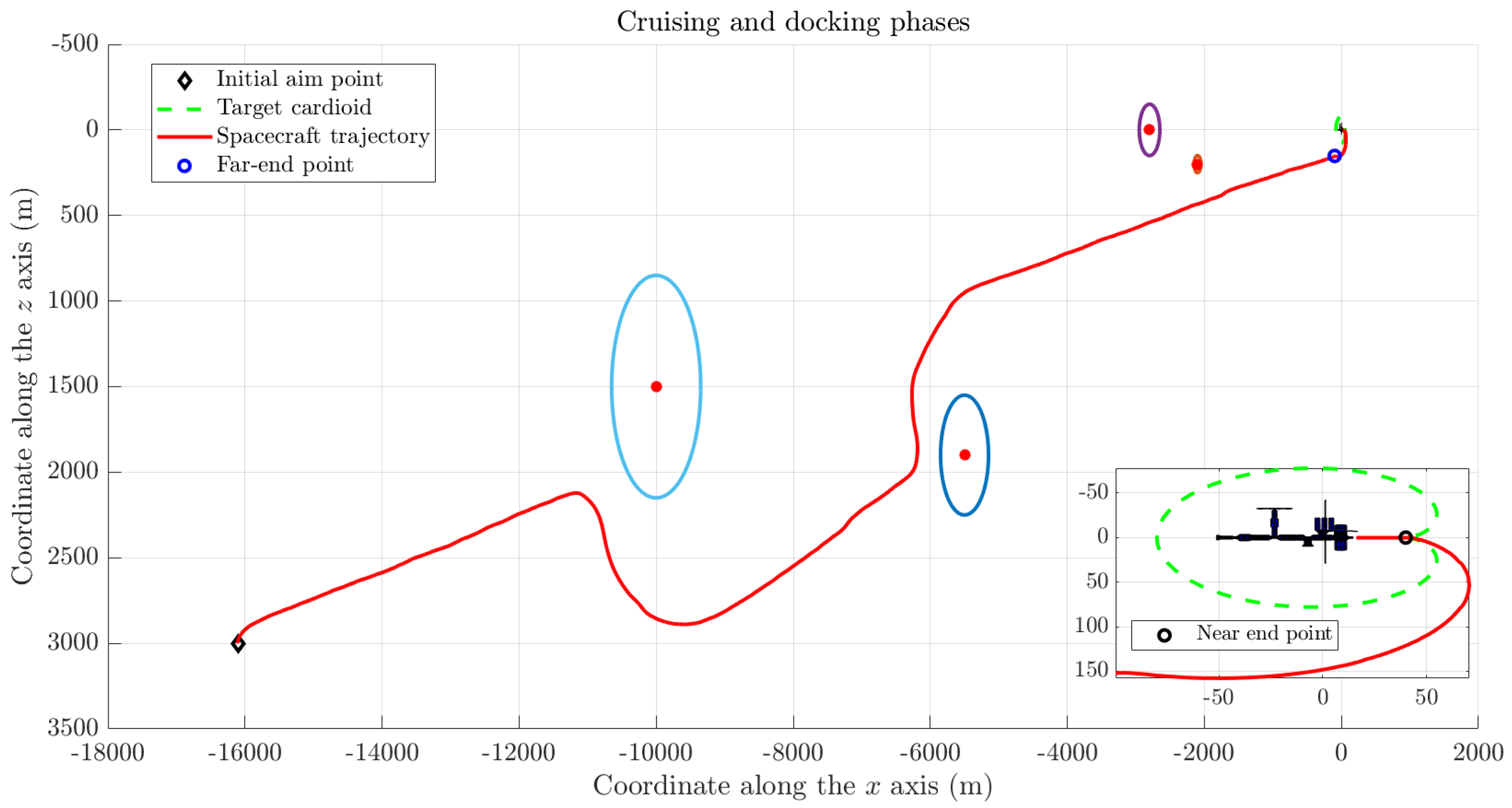
  • As to what concerns positional control, in the present endeavor, we checked and corrected the sliding model control strategy to properly take into account the current attitude of the spacecraft during maneuvering, which is essential given that the thrusters are fixed to the hull of the spacecraft. Moreover, we modified the shape of the artificial potentials that guide the motion of the spacecraft and designed different control laws, with the aim of improving maneuverability and to diminish cold gas consumption. Such control laws are contrasted to each other by numerical simulations in order to determine which one is most suitable in a rendezvous scenario. In addition, we incorporated a cardioid-shape barrier to the pure artificial potential control strategy to benefit from both techniques at once.
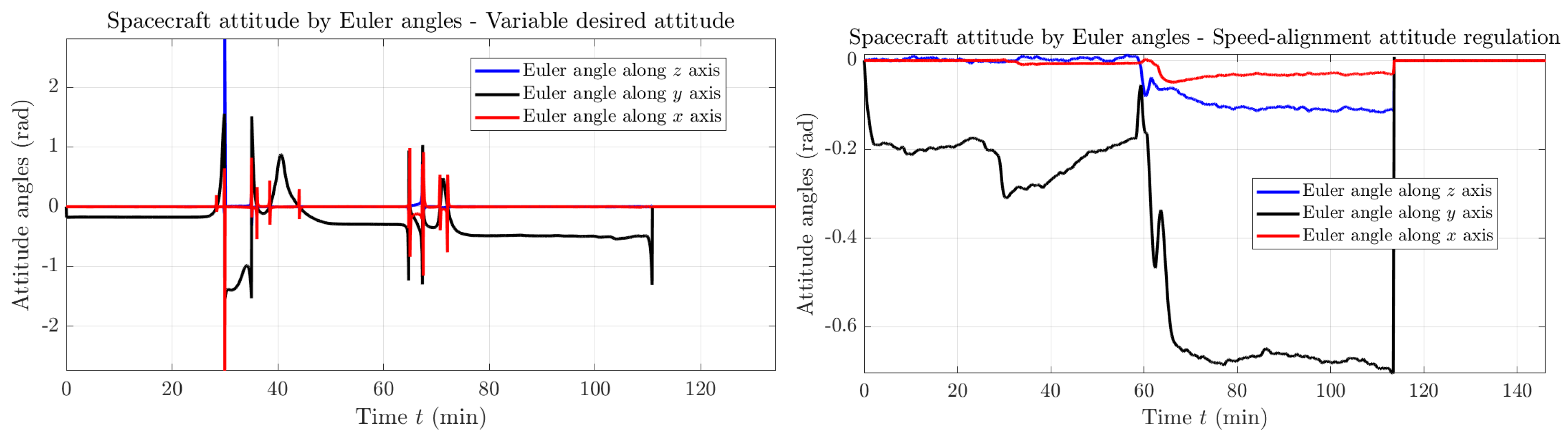
  • As to what concerns attitude control, a distinguishing feature of the present authors’ research activity is that orientations in space are represented by rotation matrices and that the attitude control strategies are represented by vector fields on the tangent bundle of the special orthogonal group, in contrast to the cumbersome quaternion representation. These entities are treated as a whole, without any reference to any basis or local coordinate system. As to what concerns the choice of attitude control law, even in this case, a number of different strategies are contrasted to one another by numerical simulations in order to discriminate the best-performing one in the present scenario.
In summary, the aim of the present research in spacecraft–station rendezvous is to blend some of the best practices in the specific literature and to enrich them by our own solutions.
The present document is organized as follows. Section 2 recalls a number of notions from orbital dynamics, such as the set of reference frames used to describe the equations of motion and the sort of guidance systems available within a small-sized spacecraft. Section 3 of this document discusses the rendezvous of the spacecraft with the main station by breaking down a rendezvous maneuver task into three subtasks, namely, cruising in the presence of (possibly moving) obstacles, far-end and near-end docking. Each subtask is discussed and tackled separately through an appropriate control strategy adapted to the required degree of precision needed. The general control strategy follows a speed control paradigm, based on sliding mode control, aided by virtual attractive-repulsive potential theory. Section 4 aims at clarifying the theoretical content of the paper through a number of numerical simulations that encompass interesting cases of rendezvous. Section 5 concludes the present paper and suggests a number of possible improvements to the current state of the art to be implemented in future research studies.

2. Reference Frames, Physical Model and Equations of Motion of a Spacecraft

The present section recalls essential details about the reference frames used to describe the equations of motion of a small-sized spacecraft and the kind of propellers that allow such motion. In addition, the present section treats the numerical adaptation of the mathematical model of orbital motion on a computing platform for numerical simulations purposes.

2.1. Application Scenario and Reference Frames

The scenario taken into consideration in the present research endeavor involves a main station, which is assumed to stay in a stable orbit around the Earth and to be controlled directly by a ground station or by on-board personnel and is hence operated independently. The scenario also involves a small-sized unmanned spacecraft, illustrated in Figure 1, endowed with an on-board autonomous control system that is able to provide appropriate guidance and control actions.
In the examined scenario, the spacecraft, whose control is the main subject of the present investigation, is supposed to be endowed with two series of actuators, namely, a series of cold-gas-based reaction thrusters that affect its translational dynamics and a series of reaction wheels that affect its rotational dynamics [3]. (We just briefly mention that electrical thrusters, in place of traditional reaction-based thrusters, are currently being developed [25,26] in the context of dedicated projects).
We shall herewith assume that the number and disposition of thrusters and wheels are appropriate to make the spacecraft fully operated, namely, to ensure that the control actions generated by the devised control algorithm find appropriate realization. As to what concerns the cold-gas-ejecting thrusters, it is assumed that their thrust cannot be modulated and is either null (when ‘off’) or maximum (while ‘on’). Conversely, it is assumed that through the reaction wheels it is possible to generate any level of active torque along the three principal axes of the spacecraft. This implicitly means that no saturation on either angular momentum or torque of the reaction wheels was considered. Details on the reaction wheel assembly used to control the attitude are missing from the present treatment, since the present paper focuses on the control-theoretic aspects of the rendezvous problem under the proviso that any reasonable torque-request from the control algorithm may be promptly generated by the actual reaction-wheel system. In a more accurate simulation scenario, such information should be added to the description, these factors being a limit of the control capability of the spacecraft. (Special instances of under-actuated systems were studied, e.g., in [27]).
A station-fixed reference frame F S is instrumental. This reference frame is integral to the space station and plays a fundamental role during rendezvous maneuvers and docking, since in this phase the spacecraft takes, as a docking reference, the orientation of the axis of the port that it is assigned to. The station-fixed reference frame F S is sometimes referred to as ‘local vertical, local horizontal’ (LVLH). Of the three orthogonal axes of the reference frame F S , one is directed from the center of the station to the center of the Earth ( R bar or Z LVLH ) and is associated with a unit-vector e z : = [ 0 0 1 ] , one is directed tangentially to the orbit in the direction of motion ( V bar or X LVLH ) and is associated with a unit-vector e x : = [ 1 0 0 ] . A third axis (labeled either H bar or Y LVLH ) is oriented so as to form a right-handed frame with the former two. The symbol   denotes matrix transpose.
A spacecraft-fixed reference frame F C is introduced as well, which serves to describe its relative orientation and location with respect to the station-fixed frame F S (the subscript ‘C’ stems from the fact that, in the rendezvous literature, the spacecraft is often referred to as the chaser). The Cartesian axes of the reference frame F C are assumed to be aligned with the principal axes of inertia of the spacecraft. The relative orientation and location of the frame F C with respect to the frame F S enter the control goals to be fulfilled by the spacecraft.

2.2. Physical Model and Equations of Motion

Under the assumption that the station and the spacecraft are both orbiting the Earth at slightly different quotas, the translational motion of the spacecraft in the station-fixed reference frame F S may be described through the Clohessy–Wiltshire equations. The Clohessy–Wiltshire equations describe a simplified model of orbital relative motion, in which both the station and the spacecraft are in a circular orbit. The Clohessy–Wiltshire model provides a first-order approximation of the motion of a spacecraft in a station-fixed reference frame [28] and is widely utilized in the simulation and regulation of the guidance of small spacecrafts.
Denoting by p R 3 the coordinate vector of the centerpoint of the spacecraft with respect to the station-fixed reference frame F S , the Clohessy–Wiltshire mathematical model that describes its dynamics reads
m p ¨ = f rt + f cc + f vd + f rd , p ( 0 ) = p 0 , p ˙ ( 0 ) = v 0 ,
where the term f rt R 3 denotes the resultant of the mechanical forces exerted by the reaction thrusters on the body of the spacecraft, the term f vd R 3 denotes the contribution of the viscous drag due to friction with atmospheric particles, the term f cc R 3 denotes the resultant of fictitious forces (Coriolis and centrifugal), the term f rd R 3 denotes the resultant of random disturbances affecting the motion of the spacecraft and m > 0 denotes the total mass of the spacecraft at a given time. The arrays p 0 R 3 and v 0 R 3 denote initial position and speed, respectively.
The fictitious force term takes the expression
f cc : = m 0 0 0 0 ω 0 0 0 0 3 ω 0 2 p + m 0 0 2 ω 0 0 0 0 2 ω 0 0 0 p ˙ ,
where ω 0 denotes the orbital rate of the main station. For a circular orbit around a central body, the orbital rate is assumed to be constant and is evaluated through the expression ω 0 = μ / r 3 , where r denotes the radius of the circular orbit traveled by the station and μ denotes a standard gravitational parameter [29] (in the present context, the standard gravitational parameter reads μ = G M , where G denotes the universal gravitational constant and M denotes the Earth’s mass).
The viscous drag is considered to be non-negligible (and constant) only in the direction of motion (corresponding to the axis V bar of the LVLH system). Hence, the braking force takes the expression
f vd : = 1 2 ρ V 0 2 S C D sign ( p ˙ e x ) e x ,
where the scalar ρ > 0 denotes the density of the atmosphere, the scalar V 0 > 0 denotes the orbital speed of the spacecraft, the scalar S > 0 denotes the frontal cross-section area of the spacecraft, the scalar C D > 0 denotes a drag coefficient and the symbol ‘sign’ denotes the signum function. The orbital speed may be written in terms of the orbital rate as V 0 = r ω 0 and is henceforth constant. As a vector, the braking force always points in the opposite direction to the direction of motion.
Other known perturbations, such as solar wind push [30], are assumed to be orders of magnitude smaller than the drag force and hence negligible. Further unknown forces acting upon the body of the spacecraft, essentially of random nature, are taken into account through the disturbance term f rd .
Although it is not necessary to the present treatment to dive into constructive details about the reaction thrusters, we highlight that a constructive detail to bear in mind is that the thrusters are arranged in such a way that two thrusters at a time are eventually switched on in order to exert a null torque on the spacecraft body. Such design aids control development since it essentially decouples translational-oriented actuation from rotational-oriented actuation. Also, such observation is essential in correctly evaluating the level of propellant consumption during each maneuver.
The instantaneous orientation of a spacecraft is described by a rotation (special orthogonal) matrix R SO ( 3 ) . This rotation matrix is defined to be the one that describes the orientation of the spacecraft-fixed reference frame F C with respect to the station-fixed reference frame F S . In the present context, the mathematical space SO ( 3 ) is regarded as a Lie group with tangent bundle T SO ( 3 ) and Lie algebra so ( 3 ) (see, e.g., [31,32]).
The rotational dynamics of a rigid body is expressed by a system of two first-order differential equations on the tangent bundle T SO ( 3 ) [10]. In particular, the rotational dynamics of a small spacecraft is described by a pair of differential equations of the following form:
R ˙ = R Ω , R ( 0 ) = R 0 , J Ω ˙ = Q Ω + T rw + T rd , Ω ( 0 ) = Ω 0 ,
where R ˙ T R SO ( 3 ) denotes the rotational speed matrix of the spacecraft in the station-fixed reference frame F S , Ω so ( 3 ) denotes the skew-symmetric angular speed matrix of the spacecraft in the reference frame F C , the symbol J : so ( 3 ) so ( 3 ) denotes the inertia operator, the operator Q : so ( 3 ) so ( 3 ) denotes the resultant of inherent torques due to inertia and mass imbalance within the spacecraft, T rw so ( 3 ) denotes the mechanical torque exerted by the reaction wheels and T rd so ( 3 ) denotes a random disturbance term. The quantities R 0 SO ( 3 ) and Ω 0 so ( 3 ) denote initial attitude and angular speed, respectively. Details on the derivation of the above equation may be found in the companion paper on spacecraft reorientation [32].
The operator J and the operator Q stem from the Euler–Poincaré equations of motion on the Lie group SO ( 3 ) . The function J Ω is linear (and invertible) in Ω , while the function Q Ω is quadratic in the matrix variable Ω . As it will be clarified in Section 3.4, as long as simulation is concerned, it is not necessary to specify the structure of the operator Q , since a fully actuated system may be controlled under the principle of dynamics replacement [19], based on inherent dynamics decoupling. In the model (4), the second equation establishes the rotational speed in the reference frame F C . The mechanical torque field T rw will depend on the actual attitude R through the chosen control law. The first equation in the system (4), often referred to as ‘reconstruction equation’, allows one to reconstruct the actual attitude of the spacecraft in the reference frame F S on the basis of the calculated angular speed.
The mass of a spacecraft changes over time due to propellant consumption during rendezvous operations. Since the total mass m > 0 enters the equations of dynamics (1), mass decay needs to be taken into account. Mass decay is described through the differential equation [33]:
m ˙ = n f ¯ rt g I sp , m ( 0 ) = m 0 ,
where m 0 > 0 denotes the initial mass of the spacecraft inclusive of payload and propellant. In the above expression, the constant scalar f ¯ rt > 0 denotes the maximum thrust of each propeller, the symbol g > 0 denotes the gravitational acceleration and the constant I sp > 0 denotes the specific impulse of each propeller (specific impulse is a measure of how efficiently a reaction mass engine creates thrust). The variable n denotes the number of active thrusters at a given time and may only take the values 0, 2, 4 and 6. (In an ideal setting, since the two thrusters responsible for the thrust in the Y LVLH direction are never activated, the case n = 6 would never occur). Indeed, Equation (5) only describes mass decay on a low-propellant-consumption regime, since the mass m eventually saturates to the ‘naked’ mass of the spacecraft.
Mass distribution also affects the rotational inertia of a spacecraft. We shall, however, assume that the contribution of the propellant mass to the total inertia is negligible; hence, the inertia operator J will be considered time-invariant. In addition, we shall consider a well-balanced mass distribution, in such a way that the inertia operator will be parameterized by a single scalar inertia coefficient J C > 0 . Such an assumption leads to the simplified relation J Ω = J C Ω .
In the following, for the sake of notation conciseness, we shall often replace the notation X LVLH , Y LVLH and Z LVLH with the shorter notation x, y and z, respectively.

2.3. Numerical Recipes

All in one, the system (4) constitutes a system of differential equations on the tangent bundle T SO ( 3 ) , while the the Clohessy–Wiltshire model takes the form of a system of differential equations in R 3 .
The Clohessy–Wiltshire model may be simulated numerically by the help of a forward Euler numerical scheme. Let us denote the discrete-time counterparts of the position vector as p s , of the linear velocity v : = p ˙ as v s , of the resultant of all forces f : = f rt + f cc + f vd + f rd as f s and of the total mass m as m s , where s = 0 , 1 , 2 , 3 , denotes an integer step counter. Denoting by h > 0 the numerical time-discretization step, the numerical scheme of choice reads
v s + 1 = v s + h f s / m s , p s + 1 = p s + h v s .
The result of such an iteration is a numerical approximation of the actual trajectory, namely, the quantity p s is an approximation of the actual coordinate vector p ( h s ) . It is worth noting that, in an ideal setting, the orbital translational motion happens on the x z plane; hence, the coordinate y would not play any role in the model. However, if the disturbances affect the motion of the spacecraft from any direction in space, a slightly off-orbit motion may be foreseen, which would need to be corrected by means of control actions. In the present paper, we shall hence make use of a full 3-DoF Clohessy–Wiltshire model.
In a similar way, upon denoting by n s the discrete-time counterpart of the number of active thrusters n, Equation (5) may be solved numerically by the iterative scheme
m s + 1 = m s n s h f ¯ rt g I sp .
To proceed with the numerical implementation of the equations in (4), we start by introducing discrete-time versions of the involved variables, namely, R s for the attitude matrix, Ω s for the angular speed matrix and T s for the total torque T : = T rw + T rd . Then, the mathematical model (4) may be integrated numerically by the scheme
R s + 1 = R s Exp ( h Ω s ) , Ω s + 1 = Ω s + h J 1 ( Q Ω s + T s ) ,
where the symbol Exp denotes the matrix exponential. The first iteration rule arises from the theory of numerical integration on Lie groups. To obtain detailed bits of information on such sort of numerical schemes, readers might consider consulting the published papers [10,19].

3. Rendezvous Maneuver under Positional Constraints

Autonomous spacecraft maneuvering toward the space station aimed at complete docking is one of the primary goals of control design in autonomous spacecraft guidance. Since guidance in the context of docking is a complex task, it is customary to break it into subtasks [3] to be separately tackled on the basis of the current physical distance between the spacecraft and the docking port. In the present research endeavor, the approaching trajectory is subdivided into three legs, namely, a cruising phase, a far-end approaching phase and a near-end approaching phase that ultimately culminates into docking.

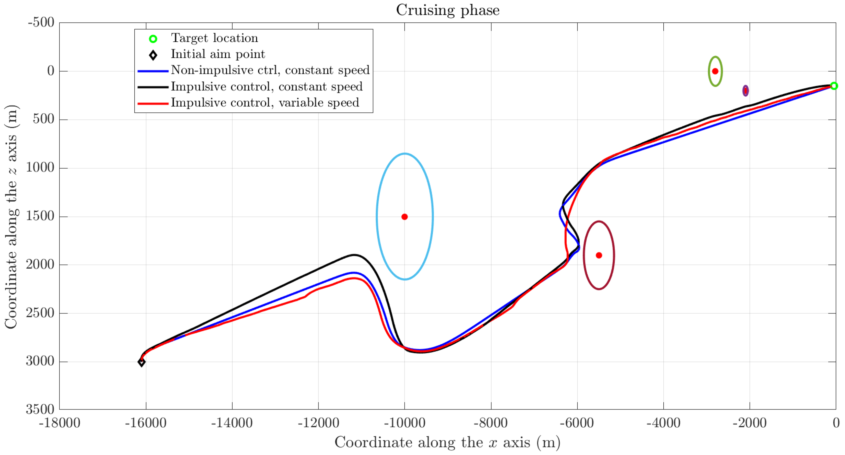
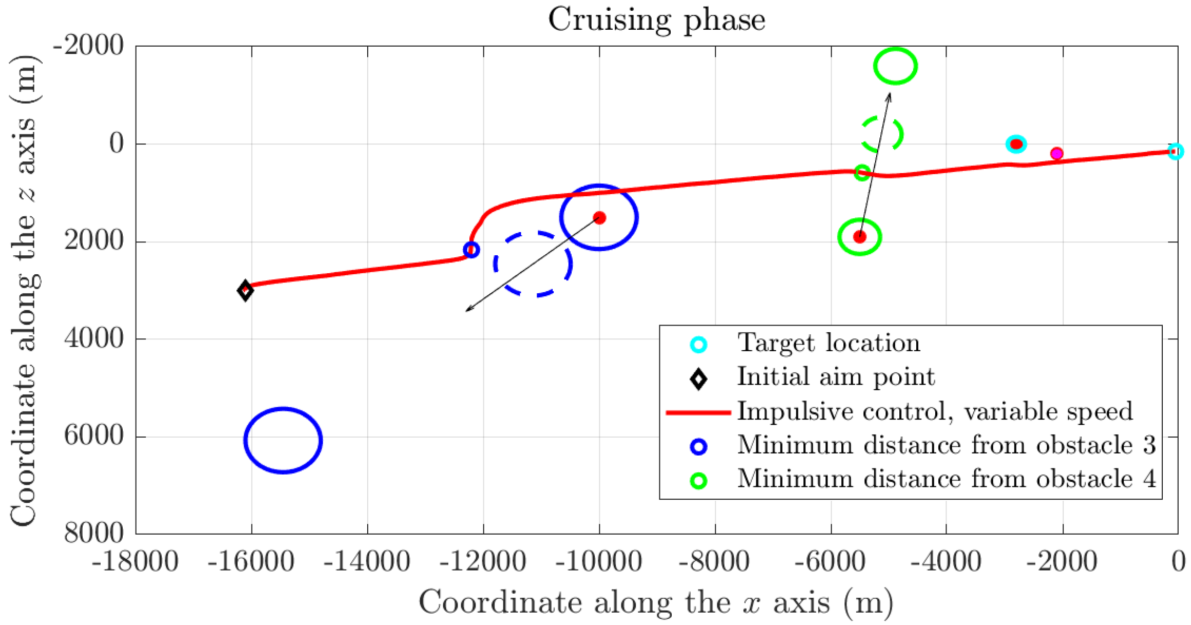
3.1. Control Strategy during a Cruising Phase in the Presence of Physical Obstacles

The maneuver of a spacecraft is required, in the presence of obstacles, to be carried out autonomously by a guidance algorithm. The algorithm devised in the present research endeavor is based on virtual attractive-repulsive potential theory and is derived in three versions: a version adapted from [3], a novel version based on impulsive control inspired by the work [1] and a further novel version that builds on impulsive control by an adaptive desired approaching speed.
Inspired by the work [3], we devised a control algorithm that switches ‘on’ the thrusters according to a first-order sliding mode control method, described by the relation:
f rt = 2 φ f ¯ rt R sign ( σ ) ,
which expresses the fact that a pair of thrusters per axis of the spacecraft are eventually switched on, hence exerting a thrust twice as large as the maximum thrust per axis. Which pairs of thrusters are switched on is determined by the sliding output vector σ R 3 , whose value is inessential except for the signs of its components. We introduced a modification to the original control equations in [3], which is reflected in the presence of the F C -to- F S reference conversion matrix R, which accounts for simultaneous position and orientation regulation, and in the addition of the variable φ { 0 , 1 } , which represents a flag to be employed in impulsive control.
In general, sliding mode control (SMC) is based on a discontinuous feedback that switches among a number of control laws according to a predefined decision rule. For a basic review of its features, readers might consult [34,35]. For a more advanced account of SMC, interested readers might consult [36], while for a more practical perspective the book [37] might prove useful.
It is worth highlighting that the force term f rt and the integer number n that appear in the expression (5) are related by
φ f rt 2 = 2 n f ¯ rt 2 ,
which, in fact, allows for determining the number of currently active thrusters on the basis of the output of the control algorithm as n = 2 sign ( σ ) .
The variable σ is made to depend on the mismatch between the current velocity p ˙ of the spacecraft and the desired velocity p ˙ d R 3 , as well as on the mismatch between the current position p of the spacecraft and the desired position p d R 3 , through the linear combination
σ : = p ˙ p ˙ d + c ( p p d ) .
Such an instance of sliding mode control is referred to as ‘component-wise SMC’ [23]. The constant c 0 determines the relative weight between position and velocity mismatch. As a matter of fact, since the information about the spacecraft’s current position enters the expression of the desired speed, we choose to set c = 0 throughout the present paper. This choice matches the preference expressed, e.g., in [23]. Alternative choices are certainly possible. In the making of the present research project, we happened to test a few alternatives to no avail.
The quantity p d is determined by the position of the target of the cruising phase, which normally is located from within a few hundreds to a few dozens of meters away from the docking port and is generally constant. The desired velocity changes along the trajectory and is determined through a virtual potential by the following expression according to [3,23]:
p ˙ d = v d p U p U ,
where p U R 3 denotes the gradient of the potential U : R 3 R , while v d > 0 denotes the desired scalar speed, determined independently of the virtual potential. As a result, it holds that p ˙ d = v d ; hence, the entity and the direction of the desired speed are determined independently of one another by the control algorithm. The potential function U in the present endeavor is chosen to be the artificial potential function that guides the spacecraft through space, according to the references [3,23], as explained in the following Section 3.2.
The cruising phase ends when the distance between the spacecraft and the desired position is less than a given threshold, namely, as soon as p p d 50 m, in the present setting.
Sliding mode control is certainly not the only control strategy mentioned in the specific literature on guidance. For instance, the paper [38] combines a gradient descent-type control strategy, enriched by a damping-type term to enhance stability, with an artificial potential strategy, based on a quadratic ‘attractive’ term and a series of barrier-type hyperbolic-cotangent-shaped terms to achieve obstacle avoidance.

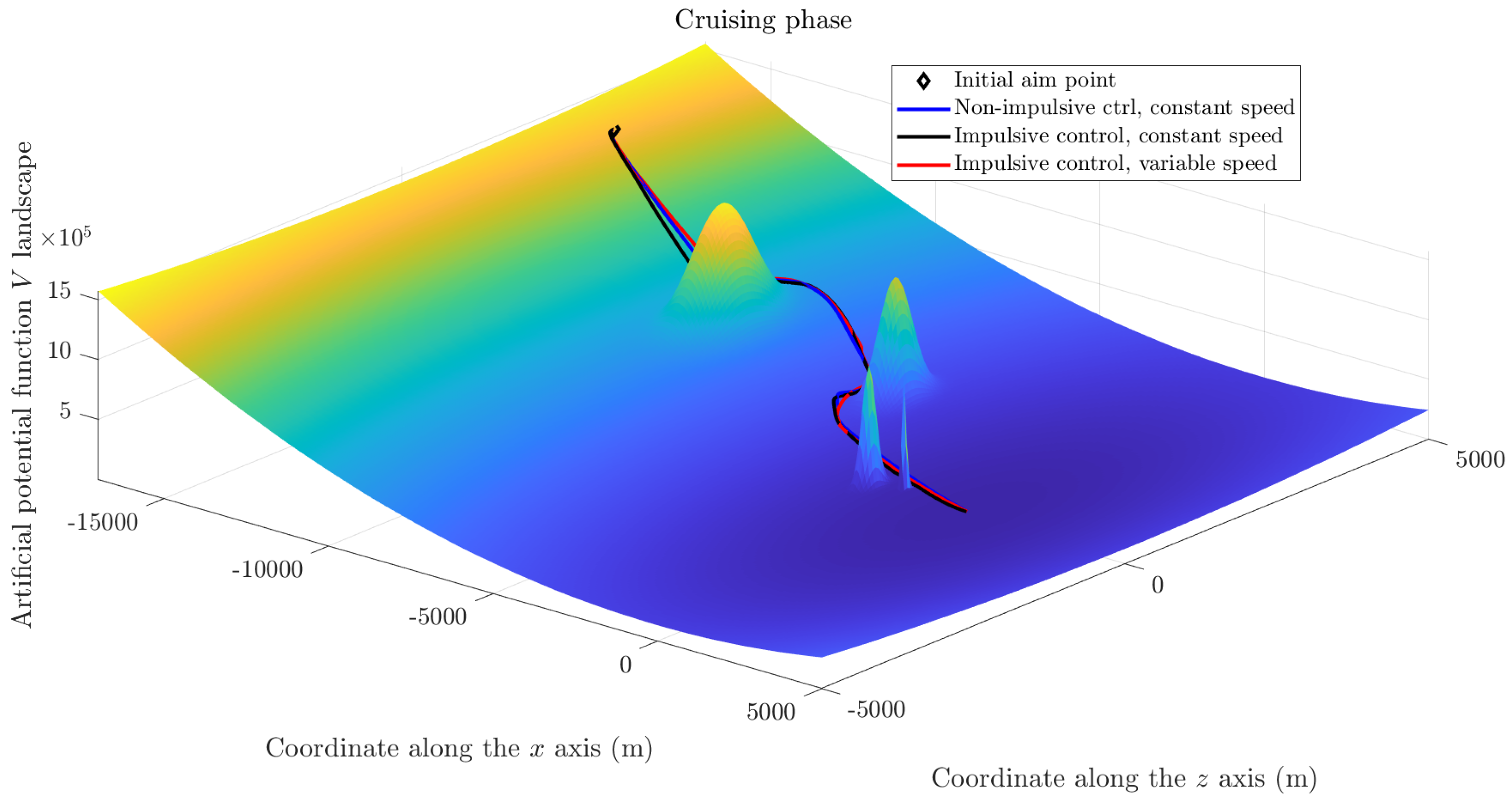
3.2. Virtual Potential Design

The virtual potential function U is designed to decrease when a spacecraft becomes closer to the target location and to increase when a spacecraft becomes closer to a physical obstacle. The gradient-based sliding mode control algorithm is hence designed to seek the minimum of the potential function.
The virtual potential is constructed as a sum of terms, one of which is ‘attractive’ and depends on the desired location, while further terms are ‘repulsive’ and depend on the location and on the safety radii of the physical obstacles. Formally, the total potential reads
U ( p ) : = D ( p ) + i P i ( p ) ,
where D : R 3 R denotes an attractive-type component and P i : R 3 R denotes a repulsive-type component. The sum runs over the number of obstacles within the approaching area between the station and the spacecraft.
The attractive-type component of the potential function is defined by
D ( p ) : = 1 2 H A p p d 2 ,
where H A > 0 is a constant that determines its relative strength. The function D ( p ) is monotonically increasing with a unique minimum in p = p d .
In order to enable the spacecraft to avoid the physical obstacles along its path to the space station, a number of repulsive-type components need to be designed that exhibit their maximum value in correspondence to the location of the obstacles and whose action peters out rapidly as the distance between the spacecraft and the obstacles increases. We shall denote as o i R 3 the location of each obstacle in the station-fixed reference frame F S and by η i > 0 the safety radius of each obstacle. Obstacles are assumed to be of spherical shape; hence, each safety radius may be thought of as the sum of the radius of the spherical obstacle augmented by an extra safety distance. On the basis of such data, the repulsive-type component of the potential associated with the ith obstacle is defined as
P i ( p ) : = 1 2 H R exp p o i 2 η i 2 ,
where the constant H R > 0 determines the strength of each repulsive term. Notice that the expression chosen represents only a soft constraint: although it cannot be ensured that the spacecraft will not enter a designated obstacle volume, a reasonable safety distance may be determined through careful handcrafting of the safety radii. It is also worth noticing that, in the present paper, the strength of each repulsive potential component is taken to be the same and to be, in particular, independent of the location and size of each obstacle.
The anti-gradient of the virtual potential function (13) reads
p U = H A ( p p d ) + H R i exp p o i 2 η i 2 p o i η i 2 .
It is important to remark that the present setting stays unvaried whether the obstacles are fixed with respect to the reference frame F S or, rather, the physical obstacles are moving with respect to the space station’s reference frame.

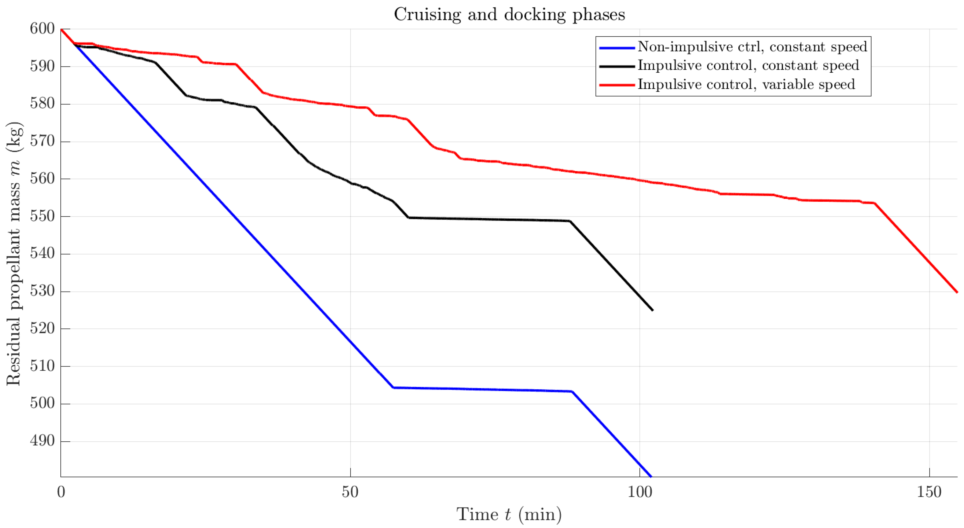
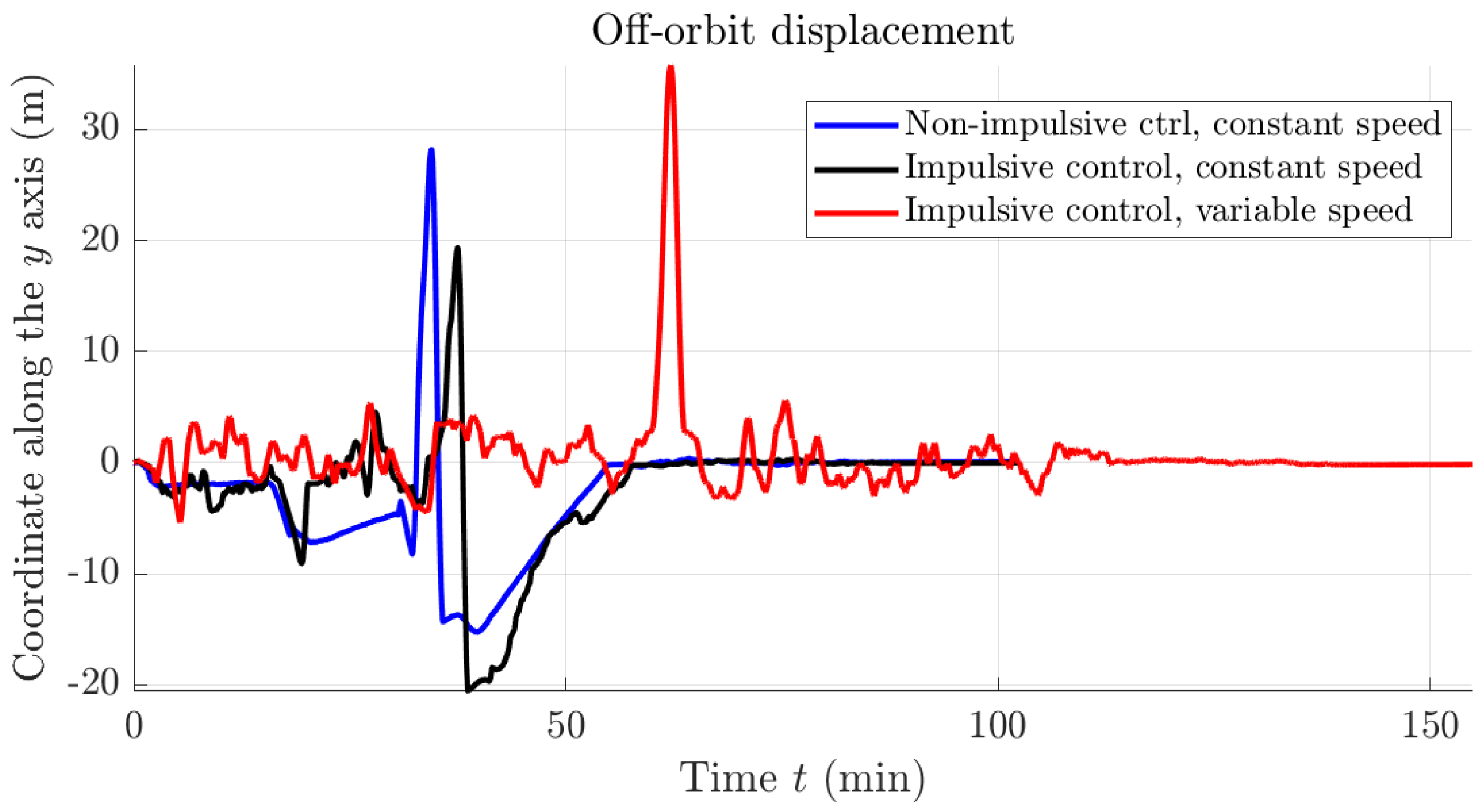
3.3. Speed Intensity Determination

The desired scalar speed may be determined on the basis of different criteria. In the present research work, we devised three strategies to determine such speed.
Non-impulsive control, constant desired speed. The simplest strategy from a computational standpoint was drawn from Reference [3] and consists in setting the desired speed to the maximum allowable speed v ¯ > 0 and the flag φ to the ‘on’ state permanently, namely,
v d = v ¯ , φ = 1 .
The upper bound v ¯ sets a limitation on the cruising speed, often dictated by safety reasons rather than technological issues. Keeping the flag φ at 1 implies that the opening and closing of reaction thrusters’ nozzles is determined solely by the SMC algorithm, which explains the name of ‘non-impulsive’ control strategy.
Impulsive control, constant desired speed. The next strategy examined was inspired by the notion of impulsive control discussed in [1] to save propellant, hence making a rendezvous maneuver safer. It consists of switching on the reaction thrusters only when the spacecraft effectively goes off the right track to the station, hence keeping them off whenever a thrust is not necessary, with the aim of saving cold gas propellant. In order to establish whether a spacecraft is moving in the right direction or rather it needs to be pushed back on track, the following quantity is defined:
Δ : = p ˙ p ˙ + p U p U .
The above scalar denotes the magnitude of the difference between the actual direction of motion and the desired speed direction as defined in Equation (12). The variable desired speed-based control strategy hence reads
v d = v ¯ , φ = 1 , if Δ > τ , 0 , otherwise ,
where τ > 0 denotes a predefined threshold that determines the sensitivity of the algorithm to a mismatch in direction. We empirically found that the threshold should be of the order 10 2 to obtain good results. In fact, we set τ = 0.05 throughout this paper. Notice that this strategy only influences the ‘off’ state of the thrusters, while it does not influence the ‘on’ state.
Impulsive control, variable desired speed. An allegedly more proficient strategy also influences the ‘on’ state of the thrusters by determining the speed amplitude. The novel law we suggest to determine speed is such that the closer the spacecraft is to the target, the smaller the cruising speed results to be. In formulas, we have:
v d = min { v ¯ , 5 p p d 1 4 Δ } , φ = 1 , if Δ > τ , 0 , otherwise ,
where the variable Δ is defined as in Equation (18). The relationship to determine the desired speed intensity was empirically handcrafted by trial and error. The hard-limiting check on the speed prevents the computed speed from exceeding its maximum allowable value.

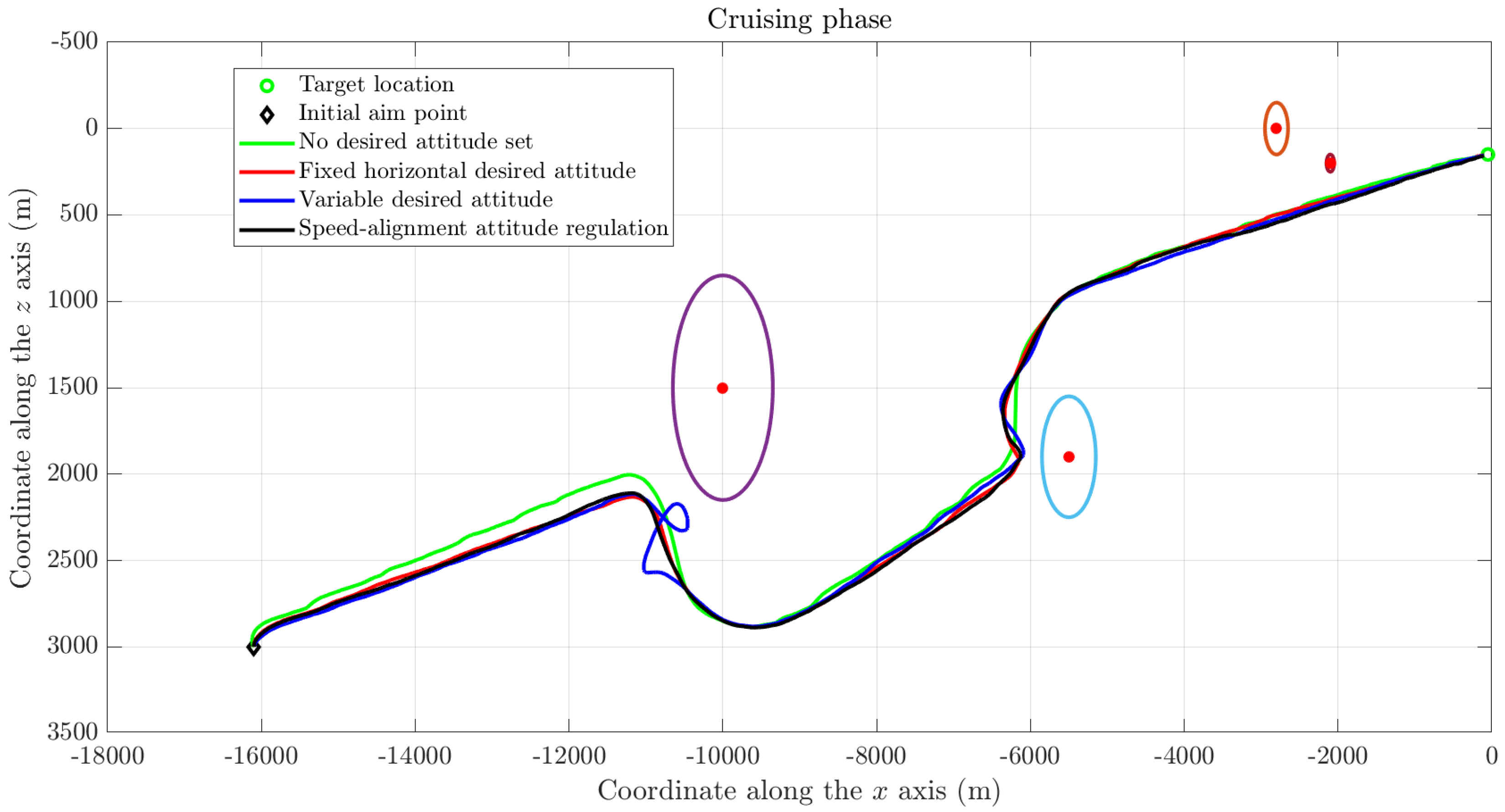
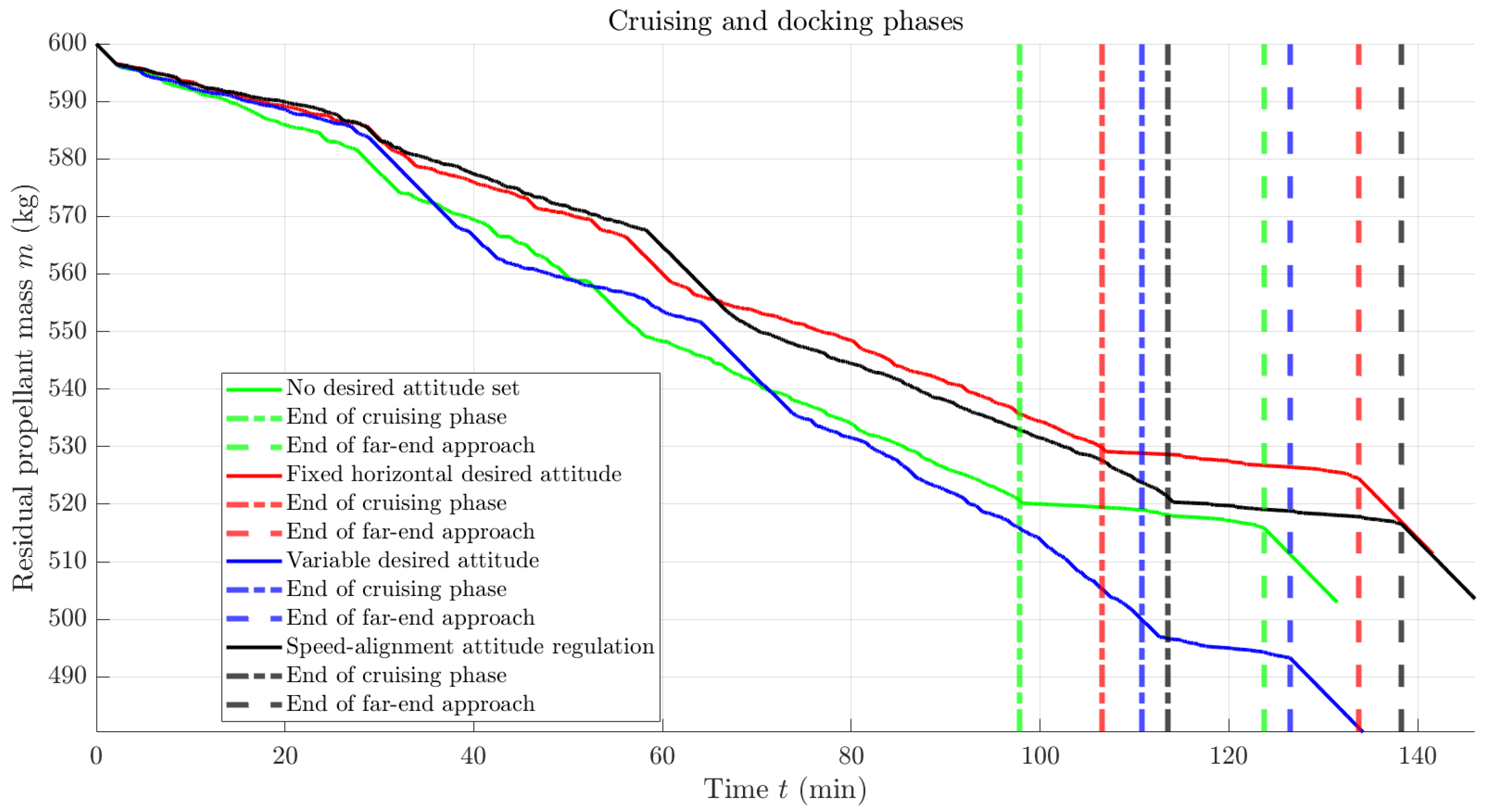
3.4. Attitude Control during a Cruising Phase

During the cruising phase, it is not essential to control the attitude of a spacecraft, which may keep a constant orientation resulting from the terminal state of previous maneuvers, until the beginning of the docking phase. Nevertheless, to aid the stability of a spacecraft against unforeseen events [3], in the present research endeavor, we deemed it appropriate to explore a number of attitude regulation strategies. In practice, a slight misalignment might certainly be tolerated, even during docking, as it is the case in different kinds of operations [39].
A way to control the orientation of a spacecraft during the cruising phase is to establish a desired attitude indicator matrix R d SO ( 3 ) and to set up a control strategy to make sure the actual attitude indicator matrix of the spacecraft R SO ( 3 ) adheres to the desired attitude. In order to control the attitude of the spacecraft, a control torque is chosen according to synchronization theory [11] to be
T rw : = Q Ω K f Ω K S Log ( R d R ) ,
where the constant parameter K S > 0 determines the strength of the control action related to the difference between the current attitude and the desired attitude, while the constant parameter K f > 0 determines the strength of an artificial braking effect on the rotational motion, introduced with the purpose of stabilizing the motion of a spacecraft. (Notice that the term K S Log ( R d R ) stems from the Riemannian gradient R of a potential function 1 2 K S d 2 ( R , R d ) and may be recognized as the ‘proportional’ component of a Lie group-type PID controller [11]). As to what concerns the determination of the desired attitude, we explored two possibilities.
Fixed ‘horizontal’ desired attitude. A first attempt consists in setting up a fixed attitude matrix that coincides with the one required for docking, namely, R d = I 3 . One such choice would lead the spacecraft to keep a fixed ‘horizontal’ attitude with respect to the LVLH reference system, namely, it would keep the axes of the reference frame F C aligned to the axes of the reference frame F S . In this way, the spatial attitude of the spacecraft coincides at all times to the orientation attitude required for docking and a spacecraft does not need to be reoriented in close proximity to the docking port. We should underline that, in a real-world scenario, such a choice might be unfeasible since the attitude control of the spacecraft might be affected by a limited control accuracy.
Variable desired attitude. As a second attempt, the desired attitude was set up to be the one that corresponds to the direction of the desired speed p ˙ d , as defined in (12). The relation between the resulting (time-varying) matrix R d and the components of the desired speed vector p ˙ d may be found in [3], in Equations (14)–(17). In such reference paper, the desired orientation with respect to the LVLH frame is obtained by calculating the orientation (Euler) angles with respect to the LVLH frame on the basis only of the three Cartesian components of the desired speed p ˙ d and by the orientation matrix arising from the composition of the three elementary rotations corresponding to each angle.
In addition, we deemed it appropriate to evaluate two further attitude regulation strategies that result in the torque terms described below.
No desired attitude set. A third strategy, corresponding to a lack of synchronization between the spacecraft and the space station, was tested against the former two methods. This corresponds to setting the control torque as
T rw : = Q Ω K f Ω ,
which aims at just passivating the spacecraft and at mitigating the effects of unpredictable disturbances through the braking term on the right-hand side. Such braking term is incapable of taking a spacecraft into any predefined orientation but is able to prevent it from spinning uncontrollably as a possible outcome of an unexpected collision. The above torque expression corresponds to the general expression (21) where one sets K S = 0 .
Speed alignment attitude regulation. A fourth novel strategy, loosely based on a previous proposal from the first author of the present paper and coworkers [19], consists of setting up a control torque that tends to align the speed p ˙ of the spacecraft to the desired speed resulting from the virtual potential function described in Section 3.1, namely, p U p U . The corresponding torque term reads
T rw : = Q Ω K f Ω + K V p U ( p ˙ ( p U ) ( p U ) p ˙ ) ,
where the constant parameter K V > 0 denotes the relative weight of such aligning torque. Notice that the rightmost term corresponds to the vector cross product p ˙ ( p U ) in so ( 3 ) notation, which vanishes when these vectors are parallel.
More sophisticated attitudinal control strategies may certainly be put into effect, taking into account, for example, specific unwanted and wanted directions. Such control problem was discussed in details in the companion paper [32] dedicated to the reorientation of a spacecraft under directional constraints. This sophisticated problem was, however, not considered in the present contribution.

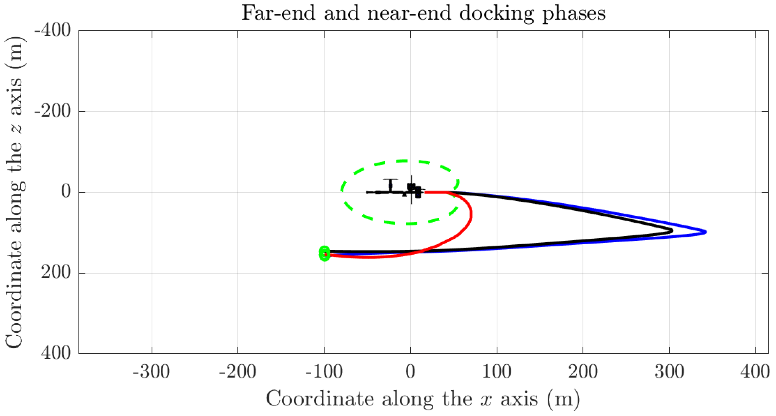
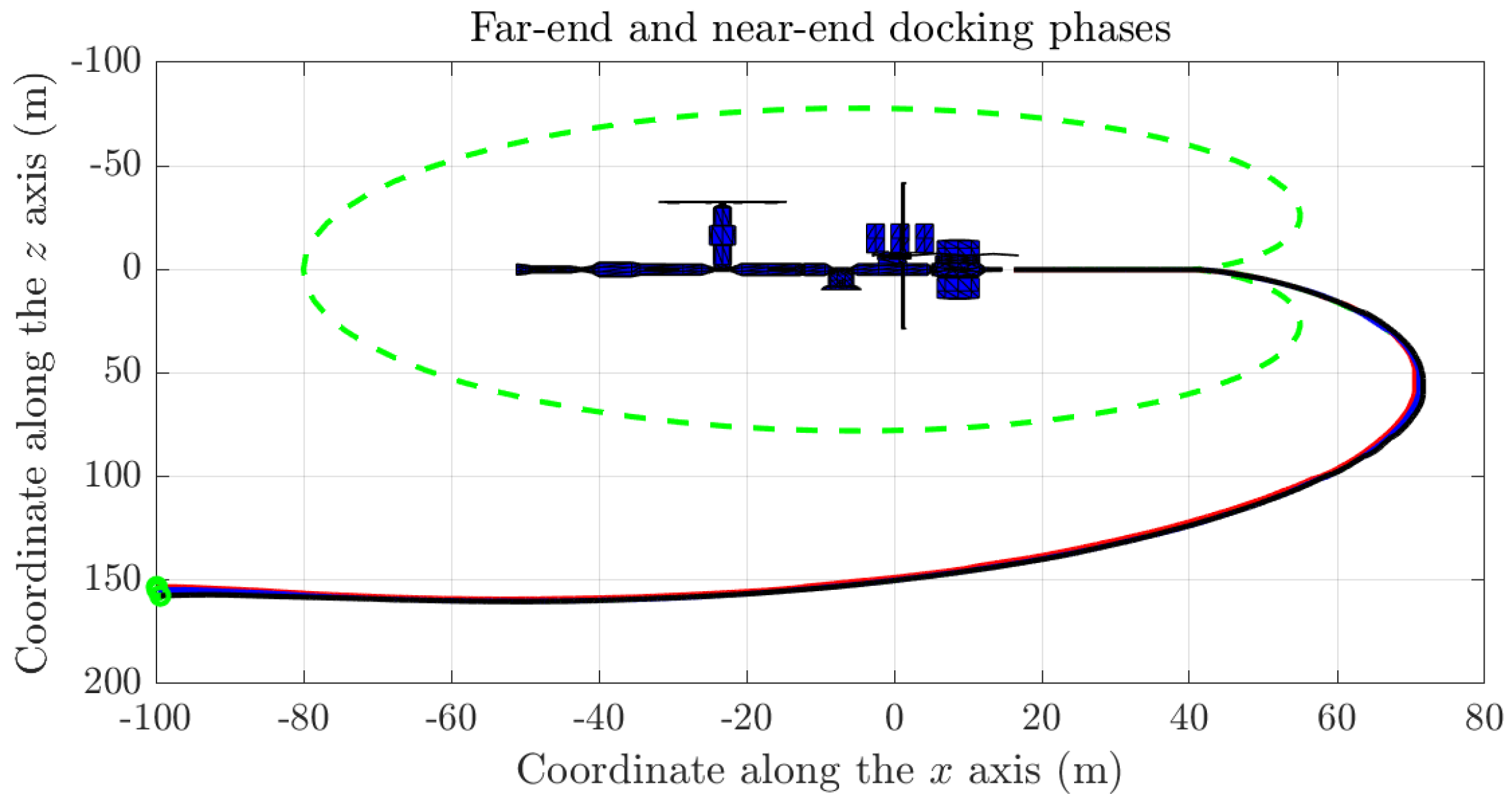
3.5. Final Guidance for Docking in the Absence of External Obstacles

Docking specifically refers to the joining act of two separate free-flying space vehicles (in contrast to ‘berthing’, which rather refers to operations where a passive module is placed into a designated interface of a second space vehicle upon being grappled by a robotic arm). In close proximity to the space station, at a distance of a few dozen meters, it is reasonable and safe to assume that no large obstacles stand in the way. During the final approach, therefore, the only obstacles to be taken into account are the outer structures of the space station itself.
In order to avoid colliding with any part of the station, a technique adapted from [1] is deployed, based on a safety zone whose border takes the shape of a cardioid curve. The characteristic radius of the cardioid must be selected so as to encompass the whole space station in order to allow a spacecraft to safely approach from every direction. The cardioid itself includes a recess, a cuspid whose tip coincides with the docking port and whose asymptote coincides with the docking axis. Once again, we underline that in a real-world scenario such an assumption might not be feasible since the orientation regulation of the spacecraft might be limited.
The actual maneuver that ultimately leads to docking is divided into two subtasks.
Far-end approaching phase of final guidance. The first subtask consists in ensuring that, irrespective of the direction of arrival, the spacecraft be positioned to the right side of the docking port while avoiding the outskirts of the space station by keeping out of the cardioid-shaped safety region.
The tip of a cardioid cusp is located at a point in space denoted as p fe R 3 in the station-fixed reference frame, and the cusp opens along the x axis. The far-end approaching phase continues until the distance between the spacecraft and the desired position becomes smaller than a given threshold, set to 1 m in the present research endeavor, namely, until p     p fe 1 m.
The cardioid curve tipping at the point p fe is defined only in the x z plane and is built from parametric equations as
x = 2 r S ( 1 cos ( 1 θ ) ) cos ( θ ) + p fe e x , y = 0 , z = 2 r S ( 1 cos ( 1 θ ) ) sin ( θ ) + p fe e z ,
where θ [ 0 , 2 π ) denotes an angular coordinate measured clockwise from the local horizon.
The angle of arrival of the spacecraft with respect to the LVLH reference frame F S is defined and calculated as
α : = π 2 atan 2 ( ( p p fe ) e x , ( p p fe ) e z ) ,
where the function atan 2 ( · ) returns the unambiguous value of the angle arising from the conversion from Cartesian coordinates to polar coordinates (see, e.g., [40]).
A preferred direction of motion is evaluated at each position p during the far-end approaching phase, as if the cardioid extends to that position, to be the tangent vector to the extended cardioid boundary. Such direction is defined and computed as
l : = H T ( sin ( α ) sin ( 2 α ) ) 0 ( cos ( α ) cos ( 2 α ) ) ,
where the constant parameter H T > 0 determines the amplitude of such tangential term.
The attractive-type term in the control vector field takes the usual affine form, namely,
a : = H Q ( p p fe ) ,
where the constant H Q > 0 denotes the relative strength of such attractive-type field.
The control strategy of choice during far-end approaching is an impulsive, variable-desired-speed regulation strategy similar to the one invoked in the description of the cruising phase, characterized by a desired-speed and flag-value pair given by
v d = min { v ¯ fe , p p fe 1 4 Δ } , φ = 1 , if Δ > τ , 0 , otherwise ,
where, in this context, the variable Δ was defined to be
Δ : = p ˙ p ˙ l + a l + a
and v ¯ fe = v ¯ 10 . Such speed limitation was chosen empirically, by trial-and-error, after evaluating a number of cases of docking maneuvers. In the above definition, the quantity Δ provides a measure of discrepancy between the actual speed direction of the spacecraft and a desired motion direction, which was defined to be proportional to the sum of the attractive-type component of the control field and of the preferred direction of motion due to the cardioid-shaped safety boundary.
Near-end approaching phase of final guidance. The second subtask is termed near-end approaching, and is meant to ensure safe and steady docking in the absence of any obstacle of sorts, except for the docking port itself. Such procedure takes, as input, the desired location p ne R 3 to drive the spacecraft to the docking port. Since the spacecraft is now aligned with the docking axis, the preferred direction of motion coincides with the direction e x during the whole near-end approaching phase.
The control strategy used in this phase is a non-impulsive variable-desired-speed-based regulation as described in Section 3.3. Such choice is motivated by the necessity of achieving the best level of precision possible in close proximity to the docking port, in the order of centimeters. In formulas, we have:
v d = min { v ¯ ne , p p ne 1 4 Δ } , φ = 1 ,
where it was made use of the further discrepancy measure
Δ : = p ˙ p ˙ + e x
which quantifies the mismatch between the actual direction of motion and the wanted direction of motion, and where v ¯ ne : = v ¯ 10 represents a speed limit believed to be valid in this phase. Even in this maneuver, the maximum allowed speed was limited to one-tenth of the speed limit allowed during the cruising phase for safety reasons.
The near-end approaching phase continues until the distance between the spacecraft and the desired position is ideally zero. In practice, considering the position p of the spacecraft as the position of its centerpoint, the near-end approaching phase terminates when the distance p     p ne is equal to the distance between the centerpoint and the juncture port of the spacecraft, up to a centimeter-order tolerance.

3.6. Alignment to a Docking Axis during Final Guidance

In order to regulate the attitude of a spacecraft during the final guidance stage, a control torque is again chosen according to synchronization theory similarly to Equation (21). During final guidance, the desired attitude of the spacecraft is constant to R d = I 3 , which describes a state of stable alignment between the reference system F C and the frame F S . Hence, the expression of the active torque may be simplified to
T rw = Q Ω K f Ω K D Log ( R ) .
The constant K D > 0 serves to determine the relative strength of the attractive-type term to the artificial friction term.

4. Results of Numerical Simulations

The present section illustrates and discusses the results of several numerical simulations performed on rendezvous maneuvers. The parameters that appear in the mathematical model of a spacecraft’s motion are summarized in Table 1. In all numerical simulations, the stepsize was set as h = 0.01 s.
In the simulations, it will be uniformly assumed that the initial angular speed is null, namely, Ω 0 = 0 . In fact, the rendezvous of spinning spacecrafts (such as powerless spacecrafts and invalid satellites) requires a specific design [38] not considered in the present endeavor.

4.1. Numerical Simulations

An initial numerical simulation was performed in the presence of obstacles with fixed location with respect to the reference frame F S . A second simulation was devoted to testing the behavior of the guidance algorithm in the presence of moving obstacles. In the first and second simulations, no attitude control took place. A third numerical simulation was, instead, dedicated to evaluating the performance of a guidance strategy that consists in joint positional and attitudinal control.
Simulation 1. The first numerical simulation was performed by assuming the presence of physical obstacles whose position is fixed with respect to the reference frame F S . The aim of this simulation was to compare the performances of the three control strategies described in Section 3.1 in terms of propellant consumption.
The initial location, desired location and initial speed of the spacecraft are summarized in Table 2, while Table 3 shows the location of four obstacles along with the associated safety radii. These simulation data were partially adapted from Reference [3]. In this numerical simulation, the components of the random disturbance F rd are zero-mean random Gaussian variables with a standard deviation of 100 N. Notice in particular that the random disturbance takes a non-zero component even along the y axis; henceforth, the motion of the spacecraft will take place slightly off the x z plane and the control algorithm will need to compensate for this unwanted effect (the desired position is located on the local vertical plane, in fact).
Numerical results concerning the cruising phase in Simulation 1 are illustrated in Figure 2, which shows the trajectory of the spacecraft along the x z plane in the LVLH coordinate frame, and in Figure 3, which shows the trajectory of the spacecraft superimposed on the landscape of the virtual potential function used to achieve automated guidance.
In particular, Figure 2 shows how the spacecraft is enabled to traverse the space, keeping sufficiently far from the obstacles while approaching the target location. The results displayed in this figure show that, far away from the obstacles, the spacecraft is driven to take the shortest route, while in the vicinity of the obstacles the spacecraft is forced to turn around the safety horizon of the obstacles found on its path, hence taking a detour from a straight line. The degree of curvature depends on the chosen values of the parameters and on the safety radii of the obstacles.
Likewise, Figure 3 serves to illustrate the shape and the function of the devised potential surface. The landscape of the potential presents a global minimum corresponding to the desired location p d as well as four peaks in correspondence to the obstacles’ central locations o i . The trajectory of the spacecraft develops across areas of higher potential while ‘rolling down’ toward the minimal-potential location.
Such results were obtained by setting the values of the parameters, as defined in the context of an attractive-repulsive potential in Section 3.2, to H A = 10 2 and H R = 10 6 . The obtained trajectories appear quite similar to one another and the three control strategies are able to lead the spacecraft toward the target location where the cruising phase ends.
However, the consumption of propellant resulting from the application of the three control strategies appears to be quite different. Cold gas consumption resulting from the three regulation strategies is displayed in Figure 4. The introduction of impulsive control results in a significant reduction in propellant consumption compared to non-impulsive regulation. Furthermore, the decay of total mass corresponding to the regulation algorithm based on impulsive control and variable desired speed compared to the constant speed case corresponds to a further saving in propellant consumption during the cruising phase.
A further element of the evaluation of the control strategies under comparison is the final speed upon reaching the predefined target location. No control requirements were defined on this matter; hence, the control strategies do not embody any information about final speed at the target location. However, the regulation strategy based on variable speed implicitly makes the final speed vanish to zero since the desired speed is proportional to the distance to the target. The effects of explicit speed limitation are illustrated in Figure 5, from which it is apparent how, in this instance, the spacecraft arrives ready to start the docking sequence, while control strategies based on constant speed ‘shoot’ the spacecraft excessively far away from the space station, an issue that seemingly were left unattended in the cited previous works.
The position at which the far-end maneuver stops is indicated as p fe = [ + 75 0 0 ] (m), while the position at which the near-end maneuver stops is indicated as p ne = [ + 15 0 0 ] (m). Notice that the final target p ne is located 15 m behind the centerpoint of the station—whose coordinate in the F S system is [ 0 0 0 ] by definition—to comply with the actual position of the docking port. The values of the parameters to deploy a cardioid-shaped safety zone, as defined in Section 3.5, were set to H T = 1 , H Q = H A and r S = 30 m.
Because of the above-mentioned evaluation elements, we deemed it appropriate to perform the subsequent simulations only on the basis of the devised impulsive-control-type, variable-speed-based regulation strategy.
Since in the devised numerical simulations a disturbance is present even along the y axis, it is interesting to evaluate the effects of this disturbance on the ability of a spacecraft to adhere to the orbital plane. Figure 6 shows the effects of the disturbances on the y coordinate of the spacecraft in the LVLH reference frame. The control strategies were not designed with an explicit goal to keep the motion of a spacecraft over the vertical ( x z ) plane, but the final guidance procedure implicitly attains this goal. From Figure 6, it is easy to notice the presence of a high peak on the coordinate of the spacecraft along the y axis corresponding to the impulsive, variable-speed control strategy, generated by the control algorithm in the proximity of the first obstacle along the spacecraft trajectory. This effect is a consequence of the repulsive force, which takes a large value due to the radius of the first obstacle, combined with random disturbances.
Simulation 2. The numerical results obtained by letting the two largest obstacles move are illustrated in Figure 7, which shows the trajectory of the spacecraft along the x z plane in the LVLH coordinate frame. In the present numerical simulation, the two largest obstacles (which appear in blue color and in green color in the figure) are assumed to travel at constant speed with respect to the space station. In particular, the speed of the largest obstacle in the x z plane is 1 m/s, while the speed of the second-largest obstacle is 0.5 m/s.
As it may be readily appreciated from Figure 7, even in the presence of moving obstacles affecting the cruising phase, the guidance algorithm performs as expected and drives the spacecraft toward the target point, while effectively avoiding the physical obstacles on its path to the space station. In the figure, two open circles mark the points on the spacecraft trajectory of minimal distance to the moving obstacles, and the dashed ovals correspond to the actual location of the obstacles corresponding to such minimal distances. Such distances are far larger than the safety radii of such obstacles, confirming that there is no contact between the spacecraft and the obstacles.
Simulation 3. The purpose of the third numerical simulation on spacecraft cruising was to evaluate how joint position/orientation regulation affects the performance of the devised SMC-based spacecraft guidance algorithm.
In the present simulation, in addition to random disturbance on the total thrust on the spacecraft body, random disturbances on the mechanical torque affecting the orientation of the spacecraft were taken into account. In particular, the three independent entries of the term T rd were chosen to be zero-mean Gaussian random variables of standard deviation 0.01 N·m.
Four attitude regulation control torque fields were tested, corresponding to the cases discussed in Section 3.4. The values of the parameters in this simulation were chosen to be K S = 2.5 J C , K V = 0.002 J C and K f = 2.5 J C . (The control parameters were parameterized as units or fractions of the inertia coefficients J C for convenience).
The obtained numerical results are illustrated in Figure 8, which shows the trajectory of the spacecraft along the x z plane in the LVLH coordinate frame. From this figure, it clearly appears that the variable desired attitude strategy fails in the proximity of the largest obstacle. On the other hand, the strategy based on not setting a desired attitude, the one based on a fixed (horizontal) attitude and the one based on velocity alignment perform similarly to one another.
The above results tell us that the best-performing control strategy corresponds to setting a constant desired attitude (which, in the present endeavor, was chosen to be the docking orientation). It should be, however, recognized that the strategy that entails the least consumption of electrical energy consists in not operating the reaction wheels at all during the cruising phase, hence leaving the spacecraft at the mercy of inertia and little accidental impacts.
During the docking maneuver, both position and orientation regulation are of prime importance, to guarantee that the spacecraft will be able to approach the selected docking port of the space station at the prescribed location and at the right incidence inclination.
Figure 9 shows the trajectory of the spacecraft along the x z plane in the LVLH coordinate frame during a docking phase. From the figure, it is readily observed that in all cases the trajectory of the spacecraft keeps well behind the safety contour during the far-end approaching phase, while the near-end approaching maneuver drives the spacecraft straight behind the docking port.
As a further element of evaluation, Figure 10 shows the velocity of the spacecraft along the x axis and along the z axis in the LVLH coordinate frame during the whole rendezvous maneuver. The velocity curves corresponding to a variable-speed, impulsive control strategy in connection with the four discussed orientation regulation methods show that the no desired attitude and variable desired attitude methods stand out negatively. Such methods, as a matter of fact, cause a sudden rise in velocity in the proximity of large obstacles.
Figure 11 shows the consumption of propellant during the whole rendezvous maneuver. Vertical lines within such figure stand as delimiters of the three different phases of rendezvous (cruising, far-end approaching and near-end approaching). From these mass decay curves, it emerges that most propellant is consumed during the cruising phase. Also, the curves show that the fixed horizontal attitude strategy causes the most limited consumption of cold gas propellant during the entire rendezvous maneuver.
In addition to the above elements to evaluate the behavior of the control strategies under examination, Figure 12 shows the orientation of the spacecraft along the entire rendezvous maneuver in terms of Euler angles computed on the basis of the attitude indicator matrix.
It is easy to notice that the speed alignment-based attitude control strategy does not stand as particularly appealing, as it leads to a very low approaching rate and, if sped up, entails an excessive disturbance to the guidance algorithm.

4.2. Illustration of a Complete Rendezvous Maneuver

Figure 13 illustrates a complete numerically simulated rendezvous maneuver, from an initial aim point to the arrival to a docking port through cruising, far-end approaching and near-end approaching.
The shown result was obtained by the variable-speed impulsive guidance control algorithm explained in Section 3.3, and as to what concerns attitude control, by the fixed horizontal desired attitude strategy described in Section 3.4. Such strategies appear to be the most suitable during the cruising phase among the ones studied in this paper (their weaknesses and strengths were evaluated in Simulation 1 and Simulation 3). The far-end and near-end approaching phases were performed as described in Section 3.5 and Section 3.6. Constant parameters take the same values as in Simulation 3. The resulting rendezvous maneuver appears steady and stable.

5. Conclusions

The goal of the present research effort was to suggest a framework to model, simulate and control a small unmanned spacecraft, orbiting in close proximity to a space station, by a modern coordinate-free approach compatible with current inexpensive and powerful on-board computing platforms. In particular, rendezvous in the presence of fixed as well as moving obstacles was tackled and simulated on a computing platform.
Obstacle avoidance has been traditionally considered a high-level planning problem, while in recent research studies part of this task has been shown to be manageable by real-time low-level control algorithms [41]. The present research study follows this modern line of thinking and is based on multi-objective optimization.
During the development of the present research, a number of issues emerged which would need closer examination, as outlined below.
The devised simulation environment takes into account a number of nuisances on the motion of a spacecraft performing rendezvous. However, every action is propagated in the relative motion framework, which implies that the differential effect, such as the one of the drag, was not considered in the mathematical model. Since the differential effect might impact on the control performance if the difference between the ballistic coefficient of the two spacecrafts involved in the rendezvous is high, the differential effect should be properly accounted for in a future endeavor.
A further aspect to pay attention to concerns the alignment of a spacecraft attitude to a docking axis during final guidance in a robust way. Currently, final guidance is performed by setting up a torque term that tends to keep the reference frame F C aligned to the frame F S irrespective of possible orientation constraints or disturbances. Attitude control during this phase may be made more robust by introducing mandatory as well as forbidden directions and by enriching the torque control field by components related to such directional constraints.
A question that certainly will need to be addressed concerns how to estimate the values of the position p and of the velocity p ˙ on-board. Even in the case of cooperative scenarios, in which there exists an exchange of navigation data, a navigation error should be considered, since this estimation error unavoidably degrades the achievable control performance.
On the same line of reasoning, it might be noticed that a cardioid laid over the x z plane protects the spacecraft only from accidents on the orbital plane. A more complete protection would require a 3D safety surface not to be trespassed, which might be obtained, e.g., by revolving a cardioid around its symmetry axis (which coincides with the docking axis).

Author Contributions

Conceptualization, S.F., F.R., L.S. and E.S.; software, F.R., L.S. and E.S.; writing—original draft preparation, S.F., F.R., L.S. and E.S.; writing—review and editing, S.F.; supervision, S.F. All authors have read and agreed to the published version of the manuscript.

Funding

This research received no external funding. The present paper summarizes the results of an independent project conducted and ended in 2023.

Data Availability Statement

The values of the parameters used in the numerical simulations are reported within the manuscript.

Acknowledgments

The authors would like to gratefully thank Toshihisa Tanaka (Tokyo University of Agriculture and Technology—TUAT, Japan) for hosting them at the Department of Electrical and Electronic Engineering of the TUAT (Koganei campus) during March–May 2023. The authors F.R., L.S. and E.S. were supported by a grant from the CampusWorld programme of the Università Politecnica delle Marche (Italy).

Conflicts of Interest

The authors declare no conflicts of interest.

References

  1. Lopez, I.; McInnes, C.R. Autonomous rendezvous using artificial potential function guidance. J. Guid. Control. Dyn. 1995, 18, 237–241. [Google Scholar] [CrossRef]
  2. Rumford, T.E. Demonstration of autonomous rendezvous technology (DART) project summary. In Space Systems Technology and Operations; Tchoryk, P., Jr., Shoemaker, J., Eds.; International Society for Optics and Photonics, SPIE: Bellingham, WA, USA, 2003; Volume 5088, pp. 10–19. [Google Scholar] [CrossRef]
  3. Bloise, N.; Capello, E.; Dentis, M.; Punta, E. Obstacle avoidance with potential field applied to a rendezvous maneuver. Appl. Sci. 2017, 7, 1042. [Google Scholar] [CrossRef]
  4. Bongers, A.; Torres, J. Orbital debris and the market for satellites. Ecol. Econ. 2023, 209, 107831. [Google Scholar] [CrossRef]
  5. NASA’s Orbital Debris Program Office (ODPO). Available online: https://orbitaldebris.jsc.nasa.gov/ (accessed on 7 January 2024).
  6. Roberson, R.E.; Schwertassek, R. Dynamics of Multibody Systems; Springer: Berlin/Heidelberg, Germany, 1988. [Google Scholar]
  7. Lee, U.; Mesbahi, M. Feedback control for spacecraft reorientation under attitude constraints via convex potentials. IEEE Trans. Aerosp. Electron. Syst. 2014, 50, 2578–2592. [Google Scholar] [CrossRef]
  8. Hu, Q.; Chi, B.; Akella, M.R. Anti-unwinding attitude control of spacecraft with forbidden pointing constraints. J. Guid. Control Dyn. 2019, 42, 822–835. [Google Scholar] [CrossRef]
  9. Cheng, H.; Gupta, K.C. An historical note on finite rotations. J. Appl. Mech. 1989, 56, 139–145. [Google Scholar] [CrossRef]
  10. Fiori, S. Model Formulation Over Lie Groups and Numerical Methods to Simulate the Motion of Gyrostats and Quadrotors. Mathematics 2019, 7, 935. [Google Scholar] [CrossRef]
  11. Fiori, S.; Cervigni, I.; Ippoliti, M.; Menotta, C. Extension of a PID control theory to Lie groups applied to synchronising satellites and drones. IET Control Theory Appl. 2020, 14, 2628–2642. [Google Scholar] [CrossRef]
  12. Fiori, S.; Del Rossi, L. Minimal control effort and time Lie-group synchronisation design based on proportional-derivative control. Int. J. Control 2022, 95, 138–150. [Google Scholar] [CrossRef]
  13. Huang, L. Velocity planning for a mobile robot to track a moving target—A potential field approach. Robot. Auton. Syst. 2009, 57, 55–63. [Google Scholar] [CrossRef]
  14. Kamon, I.; Rivlin, E. Sensory-Based Motion Planning with Global Proofs. IEEE Trans. Robot. Autom. 1997, 13, 814–822. [Google Scholar] [CrossRef]
  15. Lee, M.C.; Park, M.G. Artificial potential field based path planning for mobile robots using a virtual obstacle concept. In Proceedings of the 2003 IEEE/ASME International Conference on Advanced Intelligent Mechatronics (AIM 2003), Kobe, Japan, 20–24 July 2003; Volume 2, pp. 735–740. [Google Scholar] [CrossRef]
  16. Levine, H.; Rappel, W.J.; Cohen, I. Self-organization in systems of self-propelled particles. Phys. Rev. E 2000, 63, 017101. [Google Scholar] [CrossRef]
  17. Rimon, E.; Koditschek, D. Exact robot navigation using artificial potential functions. IEEE Trans. Robot. Autom. 1992, 8, 501–518. [Google Scholar] [CrossRef]
  18. Nguyen, B.; Chuang, Y.L.; Tung, D.; Hsieh, C.; Jin, Z.; Shi, L.; Marthaler, D.; Bertozzi, A.; Murray, R. Virtual attractive-repulsive potentials for cooperative control of second order dynamic vehicles on the Caltech MVWT. In Proceedings of the 2005 American Control Conference, Portland, OR, USA, 8–10 June 2005; pp. 1084–1089. [Google Scholar]
  19. Fiori, S.; Bigelli, L.; Polenta, F. Lie-Group Type Quadcopter Control Design by Dynamics Replacement and the Virtual Attractive-Repulsive Potentials Theory. Mathematics 2022, 10, 1104. [Google Scholar] [CrossRef]
  20. Kasiri, A.; Fani Saberi, F. Coupled position and attitude control of a servicer spacecraft in rendezvous with an orbiting target. Sci. Rep. 2023, 13, 4182. [Google Scholar] [CrossRef] [PubMed]
  21. Yang, Y. Coupled orbital and attitude control in spacecraft rendezvous and soft docking. Proc. Inst. Mech. Eng. Part G J. Aerosp. Eng. 2019, 233, 3109–3119. [Google Scholar] [CrossRef]
  22. Zappulla, R.; Park, H.; Virgili-Llop, J.; Romano, M. Real-Time Autonomous Spacecraft Proximity Maneuvers and Docking Using an Adaptive Artificial Potential Field Approach. IEEE Trans. Control Syst. Technol. 2019, 27, 2598–2605. [Google Scholar] [CrossRef]
  23. Mancini, M.; Bloise, N.; Capello, E.; Punta, E. Sliding Mode Control Techniques and Artificial Potential Field for Dynamic Collision Avoidance in Rendezvous Maneuvers. IEEE Control Syst. Lett. 2020, 4, 313–318. [Google Scholar] [CrossRef]
  24. Hua, B.; He, J.; Zhang, H.; Wu, Y.; Chen, Z. Spacecraft attitude reorientation control method based on potential function under complex constraints. Aerosp. Sci. Technol. 2024, 144, 108738. [Google Scholar] [CrossRef]
  25. Krejci, D.; Jenkins, M.G.; Lozano, P. Staging of electric propulsion systems: Enabling an interplanetary Cubesat. Acta Astronaut. 2019, 160, 175–182. [Google Scholar] [CrossRef]
  26. Levchenko, I.; Baranov, O.; Pedrini, D.; Riccardi, C.; Roman, H.E.; Xu, S.; Lev, D.; Bazaka, K. Diversity of Physical Processes: Challenges and Opportunities for Space Electric Propulsion. Appl. Sci. 2022, 12, 11143. [Google Scholar] [CrossRef]
  27. Bloch, A.; Krishnaprasad, P.; Marsden, J.; de Alvarez, G. Stabilization of rigid body dynamics by internal and external torques. Automatica 1992, 28, 745–756. [Google Scholar] [CrossRef]
  28. Clohessy, W.; Wiltshire, R. Terminal guidance system for satellite rendezvous. J. Aerosp. Sci. 1960, 27, 653–658. [Google Scholar] [CrossRef]
  29. Ries, J.; Eanes, R.; Shum, C.; Watkins, M. Progress in the determination of the gravitational coefficient of the Earth. Geophys. Res. Lett. 1992, 19, 529–531. [Google Scholar] [CrossRef]
  30. Laker, R.; Horbury, T.S.; Bale, S.D.; Matteini, L.; Woolley, T.; Woodham, L.D.; Stawarz, J.E.; Davies, E.E.; Eastwood, J.P.; Owens, M.J.; et al. Multi-spacecraft study of the solar wind at solar minimum: Dependence on latitude and transient outflows. Astron. Astrophys. 2021, 652, A105. [Google Scholar] [CrossRef]
  31. Fiori, S. Manifold Calculus in System Theory and Control—Fundamentals and First-Order Systems. Symmetry 2021, 13, 2092. [Google Scholar] [CrossRef]
  32. Fiori, S.; Sabatini, L.; Rachiglia, F.; Sampaolesi, E. Modeling, simulation and control of a spacecraft: Automated reorientation under directional constraints. Acta Astronaut. 2024, 216, 214–228. [Google Scholar] [CrossRef]
  33. Sutton, G.; Biblarz, O. Rocket Propulsion Elements—An Introduction to the Engineering of Rockets, 7th ed.; Wiley-Interscience: Hoboken, NJ, USA, 2000. [Google Scholar]
  34. Bartoszewicz, A.; Żuk, J. Sliding mode control—Basic concepts and current trends. In Proceedings of the 2010 IEEE International Symposium on Industrial Electronics, Bari, Italy, 4–7 July 2010; pp. 3772–3777. [Google Scholar] [CrossRef]
  35. Spurgeon, S. Sliding mode control: A tutorial. In Proceedings of the 2014 European Control Conference (ECC), Strasbourg, France, 24–27 June 2014; pp. 2272–2277. [Google Scholar] [CrossRef]
  36. Utkin, V. Sliding mode control design principles and applications to electric drives. IEEE Trans. Ind. Electron. 1993, 40, 23–36. [Google Scholar] [CrossRef]
  37. Shtessel, Y.; Edwards, C.; Fridman, L.; Levant, A. Sliding Mode Control and Observation; Birkhäuser: New York, NY, USA, 2004. [Google Scholar]
  38. Wei, Z.; Wen, H.; Hu, H.; Jin, D. Ground experiment on rendezvous and docking with a spinning target using multistage control strategy. Aerosp. Sci. Technol. 2020, 104, 105967. [Google Scholar] [CrossRef]
  39. Wang, G.; Xie, Z.; Mu, X.; Li, S.; Yang, F.; Yue, H.; Jiang, S. Docking Strategy for a Space Station Container Docking Device Based on Adaptive Sensing. IEEE Access 2019, 7, 100867–100880. [Google Scholar] [CrossRef]
  40. Zhang, T.; Stackhouse, P.W.; Macpherson, B.; Mikovitz, J.C. A solar azimuth formula that renders circumstantial treatment unnecessary without compromising mathematical rigor: Mathematical setup, application and extension of a formula based on the subsolar point and atan2 function. Renew. Energy 2021, 172, 1333–1340. [Google Scholar] [CrossRef]
  41. Khatib, O. Real-time obstacle avoidance for manipulators and mobile robots. Int. J. Robot. Res. 1986, 5, 90–98. [Google Scholar] [CrossRef]
Figure 1. Pictorial representation of a small spacecraft in orbit around the Moon (image courtesy of NASA).
Aerospace 11 00245 g001
Figure 2. Numerical results obtained for Simulation 1: Trajectory of the spacecraft in the LVLH coordinate frame during the cruising phase corresponding to each control strategy examined. We recall that the X (or V bar ) axis points toward the direction of motion over the orbit; hence, a negative value of the x coordinate of the spacecraft means that this is chasing the space station from behind. The ovals denote the boundaries of the safety regions surrounding each obstacle, such that the size of the ovals corresponds to the radii of the safety regions that they are associated with. Notice that the oval denote indeed circular boundaries, as explained in the main text.
Aerospace 11 00245 g002
Figure 3. Numerical results obtained for Simulation 1: Trajectory of the spacecraft corresponding to each control strategy examined, superimposed to the landscape of the virtual potential function during the cruising phase.
Aerospace 11 00245 g003
Figure 4. Numerical results obtained for Simulation 1: Cold gas consumption corresponding to each control strategy examined.
Aerospace 11 00245 g004
Figure 5. Numerical results obtained for Simulation 1: Details of the final guidance maneuver (far-end and near-end approaching) to attain docking corresponding to each control strategy examined. The color code is the same as in previous figures concerning Simulation 1.
Aerospace 11 00245 g005
Figure 6. Numerical results obtained for Simulation 1: Details of the off-orbit effect caused by random disturbances, corresponding to each control strategy examined.
Aerospace 11 00245 g006
Figure 7. Numerical results obtained for Simulation 2 in the presence of moving obstacles: The trajectory of the spacecraft in the LVLH coordinate frame. The ovals denote the boundaries of the safety regions surrounding each obstacle and the arrows indicate the direction of motion of the obstacles.
Aerospace 11 00245 g007
Figure 8. Numerical results obtained for Simulation 3: Trajectory of the spacecraft in the LVLH coordinate frame concerning the cruising phase corresponding to four attitude control strategies.
Aerospace 11 00245 g008
Figure 9. Numerical results obtained for Simulation 3: Trajectory of the spacecraft in the LVLH coordinate frame during final guidance corresponding to four attitude control strategies. (Since the z axis actually points toward the Earth, the picture looks upside down). The dashed green line represents the safety cardioid-shaped contour that the spacecraft should keep out of.
Aerospace 11 00245 g009
Figure 10. Numerical results obtained for Simulation 3: Velocity of the spacecraft in the LVLH coordinate frame corresponding to four attitude control strategies.
Aerospace 11 00245 g010
Figure 11. Numerical results obtained for Simulation 3: Cold gas propellant consumption corresponding to four attitude control strategies.
Aerospace 11 00245 g011
Figure 12. Numerical results obtained Simulation 3: Euler angles computed on the basis of the attitude indicator matrix R corresponding to four attitude control strategies.
Aerospace 11 00245 g012
Figure 13. Numerical results about a complete rendezvous: A complete maneuver resulting in the shown trajectory in the LVLH coordinate frame. The insert in the right-bottom corner shows the details of final guidance (not to scale). The ‘far-end point’ denotes the location at which far-end approaching begins, while the ‘near-end point’ denotes the location at which near-end approaching begins.
Aerospace 11 00245 g013
Table 1. Values of the physical parameters and constants entering the mathematical model of a spacecraft as detailed in Section 2.2.
ParameterSymbolValue
Initial spacecraft mass m 0 600 (kg)
Maximum allowable speed v ¯ 6 (m/s)
Inertia coefficient J C 144 (kg· m 2 )
Propeller’s thrust f ¯ rt 10 (N)
Spacecraft’s frontal areaS1.44 ( m 2 )
Drag coefficient C D 2.20 (−)
Specific impulse I sp 220 (s)
Gravitational accelerationg9.81 ( m / s 2 )
Atmosphere density ρ 10 12 ( kg / m 3 )
Orbit radiusr 6.878 × 10 6 (m)
Gravitational parameter μ 3.986 × 10 14 ( m 3 / s 2 )
Table 2. Reference values for Simulation 1. We recall that the Z (or R bar ) axis points toward the Earth; hence, a quota of + 40 m in the LVLH reference frame denotes a target location below the station (as seen from the Earth).
DescriptionValue
Initial location p i [ 16 , 100 0 + 3000 ] (m)
Initial speed p ˙ i [ 0.5 0 + 0.01 ] (m/s)
Target location p d [ 125 0 + 40 ] (m)
Table 3. Location and safety radius of each obstacle ordered by size. All obstacles happen to be located below the station (as seen from the Earth) as the spacecraft trajectory is ascensional toward the space station.
Safety Radius (m)Location (m)
η 1 = 650 (m) o 1 = [ 10 , 000 0 + 1500 ] (m)
η 2 = 350 (m) o 2 = [ 5500 0 + 1900 ] (m)
η 3 = 150 (m) o 3 = [ 2800 0 0 ] (m)
η 4 = 50 (m) o 4 = [ 2100 0 + 200 ] (m)
Disclaimer/Publisher’s Note: The statements, opinions and data contained in all publications are solely those of the individual author(s) and contributor(s) and not of MDPI and/or the editor(s). MDPI and/or the editor(s) disclaim responsibility for any injury to people or property resulting from any ideas, methods, instructions or products referred to in the content.

