Article

Rotor Performance Predictions for Urban Air Mobility: Single vs. Coaxial Rigid Rotors

1
NASA Ames Research Center, Moffett Field, CA 94035, USA
2
Department of Aerospace Engineering, The Pennsylvania State University, University Park, PA 16802, USA
3
The Johns Hopkins University Applied Physics Laboratory, Laurel, MD 20723, USA
*
Author to whom correspondence should be addressed.
Aerospace 2024, 11(3), 244; https://doi.org/10.3390/aerospace11030244
Submission received: 31 January 2024 / Revised: 14 March 2024 / Accepted: 18 March 2024 / Published: 20 March 2024
(This article belongs to the Special Issue Recent Advances in Applied Aerodynamics)

Abstract

:
This work details the development and validation of a methodology for high-resolution rotor models used in hybrid Blade Element Momentum Theory Unsteady Reynolds Averaged Navier–Stokes (BEMT-URANS) CFD. The methodology is shown to accurately predict single and coaxial rotor performance in a fraction of the time required by conventional CFD methods. The methodology has three key features: (1) a high-resolution BEMT rotor model enabling large reductions in grid size, (2) a discretized set of momentum sources to interface between the BEMT rotor model and the structured URANS flow solver, and (3) leveraging of the first two features to enable highly parallelized GPU-accelerated multirotor CFD simulations. The hybrid approach retains high-fidelity rotor inflow, wake propagation, and rotor–rotor interactional effects at a several orders of magnitude lower computational cost compared to conventional blade-resolved CFD while retaining high accuracy on steady rotor performance metrics. Rotor performance predictions of thrust and torque for both single and coaxial rotor configurations are compared to test the data that the authors obtained at the NASA Langley 14- by 22-ft. Subsonic Tunnel Facility. Simulations were run with both fully turbulent and free-transition airfoil performance tables to quantify the associated uncertainty. Single rotor thrust and torque were predicted on average within 4%. Coaxial thrust and power were predicted within an average of 5%. A vortex ring state (VRS) shielding phenomenon for coaxial rotor systems is also presented and discussed. The results support that this hybrid BEMT-URANS CFD methodology can be highly parallelized on GPU machines to obtain accurate rotor performance predictions across the full spectrum of possible UAM flight conditions in a fraction of the time required by conventional higher-fidelity methods. This strategy can be used to rapidly create look-up tables with hundreds to thousands of flight conditions using a three-dimensional multirotor CFD for UAM.

1. Introduction

Coaxial rotor systems are finding increased use and interest from several different sectors of the rotorcraft market due to their condensed packaging, higher redundancy in multirotor systems, and benefits in high-speed forward flight. Whether it be full-sized helicopters such as the Sikorsky XH-59A, X2, and S-97 [1,2,3], new light helicopter designs and urban air mobility applications for commercial transportation [4,5,6,7], or smaller unmanned systems that fly both here on Earth and explore other worlds [8,9], this configuration is continually seeing more use. The increasing demand for coaxial rotors comes along with an increasing need to understand how they operate so we can improve their efficiency and performance. A large set of conceptual, computational, and wind tunnel-based studies have been conducted to increase the knowledge base for these systems; for example, early research conducted by Gessow, Harrington, and Dingeldein at the NASA Langley Research Center [10,11,12] studied the effects of planform design and rotor–rotor interactions on rotor efficiency. Coleman later summarized both the theoretical and experimental research to date on these rotor systems [13]. In addition to Coleman’s work, Ramasamy further summarized hover data for coaxial rotors to more closely study the interference effects taking place [14]. More recently, Yeo summarized design approaches and predictive capabilities of coaxial and compound helicopter configurations [15]. For a review of rotorcraft computational fluid dynamics (CFD), the authors recommend the summary by Strawn et al. [16], while [17,18,19] provide more recent testing and analysis of multirotor aircrafts. Prior work also applied state-of-the-art computational analysis techniques based on CFD to advanced vertical-flight aircraft design and analysis tools [20,21,22,23].
Advanced CFD approaches for coaxial rotors include those using unstructured overset grids by Xu and Ye [24], vortex particle methods by Singh and Friedmann [25,26,27,28], and a mixing-plane approach to reduce computational demand by Cornelius et al. [29]. The studies of rotor spacing and rotor–rotor interactions by Lakshminarayan and Baeder [30] also provide better understanding of the highly unsteady flowfield associated with the coaxial rotor system. Additionally, validation work for comprehensive analysis of coaxial rotors was carried out by Ho et al. [31], which characterized the impact of the upper rotor to lower rotor thrust ratio on both coaxial rotor and individual rotor figures of merit.
The analyses presented throughout this work focus on a growing subset of fixed-pitch multirotor systems, i.e., small scale (less than 2 m diameter), stiff (first flap frequency > 1.5/Rev), RPM-controlled (variable speed), and with large rotor separation (spacing > D/5) for the coaxial configuration. This blade stiffness is higher and rotor spacing larger than typically analyzed for conventional helicopter design and can be representative of some electric vertical take-off and landing (eVTOL) and urban air mobility (UAM) configurations. Much research has been carried out by Silva and Johnson [32,33,34,35] to develop NASA reference vehicles to support the increase in interest for developing these types of vehicles. Some of the NASA reference vehicles have designs more like conventional rotorcrafts, but many of them are more similar to the rotor configurations discussed in this work. New studies delving further into the analysis of these vehicles range topics covering comprehensive and CFD analyses, handling qualities, system design, hazard analysis, and wind-tunnel testing [36,37,38,39,40,41,42,43,44,45,46,47]. Of particular interest to this work are recent studies of mid-air deployment and high rates of descent with these vehicles [48,49,50,51,52]. Some works have also looked at improving the design approach specifically for coaxial and octocopter configurations [53,54]. Uncertainty quantification in performance estimation has become a big topic with all of these design variables for multirotor systems. The study by Lim, Kim, and Yee [55] presents a process for propagating design uncertainties into the flight performance estimation of multirotor vehicles.
These multirotor systems are also being used for space exploration of other celestial bodies such as Mars and Titan. The successful flight of the Mars Ingenuity Helicopter in April 2021 marked the first flight of a heavier-than-air vehicle on another planet [9,56,57,58]. Currently, the Dragonfly lander is the second multicopter vehicle under development to be sent into space following in Ingenuity’s footsteps [59]. These types of planetary aerial vehicles (PAVs) have been proposed several times over the previous two decades for scientific missions and exploration of various planetary bodies in our solar system [60,61,62,63,64,65,66,67]. Following the success of Ingenuity and the awarding of the NASA New Frontiers funding to Dragonfly, a surge of renewed interest has developed around the capabilities that these vehicles bring to planetary science and exploration [68,69,70,71,72,73].
These PAVs leverage distributed electric propulsion in multirotor configurations. This setup is very much in line with the previously discussed eVTOL and UAM movements. Thus, several applications, all based on a similar configuration with similar rotor systems, are drawing much attention and funding into the rotorcraft research community. These highly complex rotor–rotor and rotor–airframe interactions do require an approach to ensure inclusion of the complex aspects of the flowfield, but the computational costs and complexity related to these higher-fidelity tools are only feasible when analyzing a handful of flight conditions. The analyses have a computational cost too high for design optimization and are not feasible for the average user. Thus, a proven mid-fidelity capability that is computationally efficient is desired to aid in the engineering design process of these multirotor vehicles.
As such, efforts have been underway to validate a methodology using GPU-accelerated hybrid BEMT-URANS CFD to predict rotor performance throughout the full spectrum of flight conditions and rotor flow states. The major developments of the CFD modeling approach for analyzing both single and coaxial rotors are summarized, including the development of a high-accuracy BEMT rotor model for coupling with CFD. Recent studies quantifying airfoil performance table uncertainty are also presented.
In this work, the Rotorcraft CFD tool, RotCFD Version 0.9.15 (Beta) 402_K07a [74,75], is used to validate the methodology through comparisons with a multirotor experimental dataset obtained by the authors. The coaxial rotor system was tested in the NASA Langley 14- by 22-ft. Subsonic Tunnel Facility in support of the NASA Dragonfly mission [59]. This work aims to characterize the hybrid BEMT-URANS methodology as a highly accurate method for predicting steady rotor performance at a several order of magnitude lower computational cost compared to conventional high-fidelity CFD approaches.
The RotCFD tool will be described in more detail in the CFD Software and Computational Resources section. Section 2 of this paper starts with a brief introduction to the CFD tool and a description of its place among other common rotor performance prediction methods. An approach for validating the methodology used and quantifying its accuracy is then discussed. The experimental test setup is then briefly described in Section 3 by the authors who obtained the data, followed by the CFD model setup in Section 4. A comparison of the results from the CFD simulations and experimental testing is then presented in Section 5. Finally, some conclusions for the applicability of this approach in multirotor design and analysis are discussed in Section 4.
The objectives of this work are as follows:
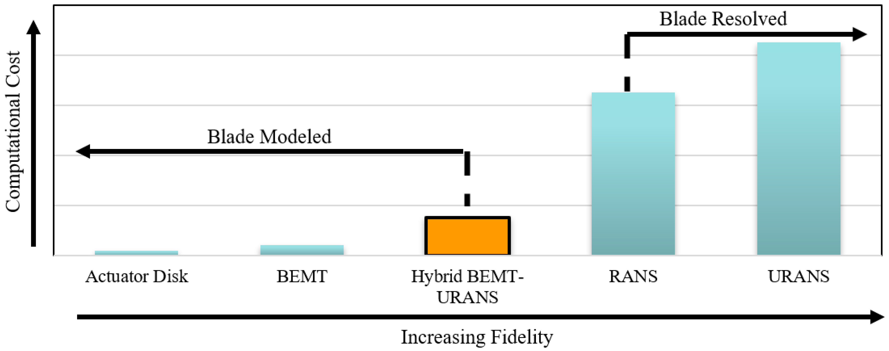
  • Summarize major developments of a hybrid BEMT-URANS CFD methodology enabling fast multirotor performance predictions.
  • Validate this methodology by comparing single and coaxial CFD rotor performance predictions to experimental data acquired in the NASA Langley 14- by 22-ft. Subsonic Tunnel Facility. Document the effects of fully turbulent versus free-transition airfoil tables on CFD rotor performance predictions using this approach.
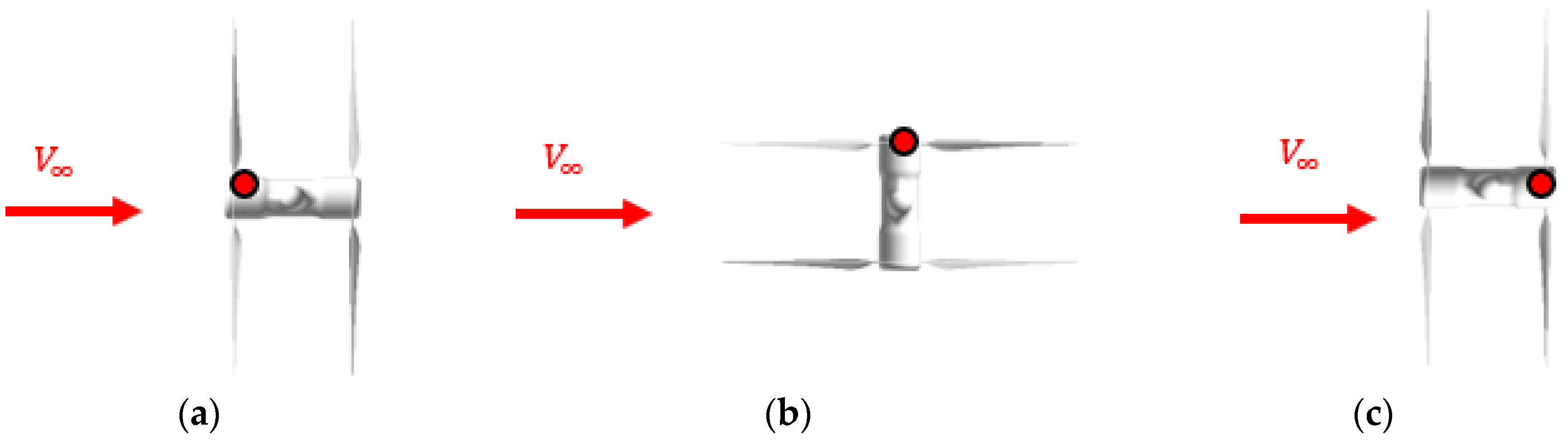
  • Provide physical insight into the coaxial rotor flow physics as a function of the rotor shaft angle (SA) from −90 degrees to +90 degrees, which is reported in increments of 15 degrees or less. Compare single versus coaxial rotor performance across a wide range of flight conditions unique to stiff, variable-speed rotor operation.

2. Computational Methods

2.1. Rotorcraft Analysis Methods

The methods considered to analyze the aerodynamic performance of rotorcrafts need to balance solution fidelity with computational cost. Several of these approaches are summarized in Figure 1, as modified from Cornelius et al. [29]. At one end of the spectrum are those methods that model the blades, which have simplifying assumptions enabling fast simulations. Examples of blade-modeled approaches are actuator disk methods and Blade Element Momentum Theory. These approaches are typically used for a preliminary design; however, if the airfoil sectional properties are unknown, or in complex interactions, these modeling methods may not have sufficient fidelity to generate a detailed design. At the other end of the spectrum are blade-resolved approaches, which include blade-resolving CFD methods such as time-accurate Reynolds Averaged Navier–Stokes (URANS) and other hybrid approaches. These approaches are referred to as blade-resolved methods because they solve a form of the Navier–Stokes equations on the true rotor geometry. These high-fidelity analysis methods directly accounting for the blade shape compute the rotor inflow at a much higher computational cost, which, in some cases, can have a solution time of several weeks on the world’s fastest supercomputers. In the middle of the chart is the hybrid BEMT-URANS methodology. This approach combines a blade-modeled description of the rotors with a time-accurate CFD resolved flowfield to achieve accuracy and computational demand suitable for engineering design. The focus of this work is to validate a multirotor CFD methodology that combines the benefits from the two categories shown in Figure 1 to achieve accurate rotor performance predictions in several orders of magnitude less time than conventional blade-resolved CFD approaches. The approach allows for the capturing of relevant aspects of the rotor system such as hub effects, rotor–rotor interactions, and the full rotor inflow and wake.

2.2. Hybrid BEMT-URANS CFD Methodology for Multirotor Systems

The RotCFD program is used to implement this hybrid BEMT-URANS methodology. The program uses a BEMT rotor model interfaced with a finite-volume structured cartesian grid system that uses implicit time integration to solve the incompressible URANS equations, a two-equation k-ϵ turbulence closure, and the SIMPLE-based solution method [76]. As compared to a lower-order blade-modeled approach with an inflow model, the URANS flowfield allows for more accurate modeling of the rotor inflow and wake trajectory in various flight conditions, as well as for the capturing of rotor–rotor and rotor–airframe interactions. The BEMT rotor model and URANS grid system are interfaced together using an actuator disk with distributed momentum sources. The URANS grid is used to calculate inflow over the entire rotor disk, which is then passed to the BEMT rotor model for use with C81 airfoil performance look-up tables. The BEMT model results are time-averaged to further reduce computational cost but retain their spatial accuracy to capture things such as retreating blade stall and advancing blade compressibility effects. The resulting BEMT sectional forces are then applied back into the URANS flowfield through the distributed momentum sources in the actuator disk. This allows for the rotor performance to be accurately modeled with a several orders of magnitude reduction in computational cost compared to blade-resolved CFD.
To include additional geometry, such as rotor hubs or an airframe, tetrahedral body-fitted cells can be implemented and have been used in the present work to model the wind-tunnel test assembly. The refinement of these cells is not typically sufficient to develop the boundary layer on any included geometry, so wall functions are used. Although boundary layers are not typically modeled, RotCFD has been shown to accurately capture the bluff-body aerodynamics critical for rotor–airframe interactions. Key information regarding the tool and prior verification efforts are provided in the reference section [77,78].

2.3. GPU Acceleration and Computational Resources

One of the most novel parts of this work is the mass parallelization of the rotor performance model on GPU-accelerated computers. RotCFD can be run using an open multiprocessing (OpenMP)-based parallelization, which is similar to the conventional approach used in high-fidelity CFD to run simulations on many Central Processing Unit (CPU) cores. Alternatively, it can be run using open computing language (OpenCL), which takes advantage of both the computer’s CPU and its graphical processing unit (GPU). Both the CPU and GPU implementations of RotCFD solve the same equations as previously described, i.e., the incompressible Navier–Stokes equations. Spatial discretization uses finite volume with implicit time integration, a two-equation k-ϵ turbulence closure, and the SIMPLE-based solution method.
GPU technology enables parallelizable mathematical problems to be completed several orders of magnitude faster than they could be completed on the CPU. GPU acceleration has not become widespread in blade-resolved CFD since the cell count is too large to fit on a single GPU, and very costly slowdowns occur during communication between GPUs and the CPU for a flow solution segmented across multiple GPUs. With the current proposed methodology of using a blade-modeled description of the rotor in a CFD resolved flowfield, however, the speed benefit achieved through GPU acceleration is roughly an order of magnitude faster than running the same simulation in OpenMP. The exact speedup depends on many factors such as CPU and GPU specifications. In general, however, the OpenCL capability allows substantially complex CFD simulations to be completed on a GPU-equipped desktop computer or even a GPU-equipped laptop in hours instead of days (or weeks). The program’s exploitation of GPU computing for rotorcraft CFD was recently investigated and reported by Rajagopalan et al. [79], who showed sampled full-vehicle simulations and the relative performance of several GPU cards in running those simulations. The present work developed an optimized GPU acceleration scripting for the hybrid BEMT-URANS methodology to attain a two orders of magnitude speedup compared to running the same simulation in OpenMP. The details of this GPU scripting and performance were recently documented by Cornelius and Schmitz [80], so only a brief overview will be provided here.
This study used two different GPU accelerators: an NVIDIA GTX 1060 (6 GB) and an NVIDIA RTX 3080-Ti. The workstation that uses the 3080-Ti, which was the fastest commercially available GPU when the simulations were run, and an AMD Threadripper 3960X 24-core CPU completes these coaxial rotor CFD simulations at 2.5 times the rate of an approximately 1500-processor computing cluster built within the Penn State Department of Aerospace Engineering in 2016. This further highlights the potential performance of a single GPU-accelerated workstation. The computing architecture allows for large CFD performance tables to be generated for various activities. One such activity is a look-up table of rotor performance to be used in the development of closed-loop simulations for flight controllers and Monte Carlo simulations for the associated uncertainty quantification. This methodology provides a suitable level of accuracy for the needs of this application while also having a low enough computational cost to have completed an 800-flight-condition three-dimensional URANS coaxial rotor CFD table in 1.5 months on a single GPU-accelerated workstation. Figure 2 is a visual of the variables parametrized in the large CFD rotor performance table, resulting in several hundred to several thousand flight conditions.
Increased parametrization through side-slip and other factors highlights the ongoing need for further advances in GPU computing and related computational cost reductions. Such a table could not feasibly be completed in a reasonable amount of time using current conventional blade-resolved CFD approaches. Further research has been conducted on both the hardware and software side of creating and operating these GPU-accelerated workstations to further parallelize the modeling approach. Thousands of these cases can now be completed per month, which has been documented by Cornelius and Schmitz [81].

2.4. Validation and Uncertainty Quantification

The purpose of this paper is to validate a hybrid approach using a blade-modeled description of rotors in a URANS flowfield for time-averaged rotor performance predictions such as thrust, power, and torque of a coaxial rotor system. To achieve this end, the authors looked for a methodology that would accomplish that goal while also quantifying the associated uncertainties within the data. A standard AIAA approach was used based on that explained by Yeo for verification, validation, and uncertainty quantification of CFD [81].
The process starts with quantifying the uncertainty of the computational model, which includes physical modeling errors, discretization errors, and convergence or round-off errors, i.e., mathematical errors tied to the simulation results. The simulation error includes the modeling error, numerical error, and input error.
δ s i m = δ m o d e l + δ n u m e r i c a l + δ i n p u t
The validation error, E % , is used to quantify the difference between the computational result, S, and the experimental result, D.
E % = S D D = δ s i m δ e x p δ e x p
Combining (1) and (2), and rearranging the result gives an expression for the model error, which is the combined error of the model trying to predict the real-world answer. It accounts for both the simulation and experimental uncertainties.
δ m o d e l = E % δ e x p ( δ n u m e r i c a l + δ i n p u t δ e x p )
In Equation (3), the validation error E % is the only known quantity. The errors on the right-hand side of the equation must be estimated. The validation standard uncertainty equation is introduced as the root sum of squares of the estimated uncertainty values from the right-hand side of Equation (3).
u v a l = u n u m e r i c a l 2 + u i n p u t 2 + u e x p 2
The numerical uncertainty encompasses discretization errors, iterative errors, and round-off errors. Typically, the iterative and round-off errors are several orders of magnitude lower than the discretization errors, so the numerical uncertainty can be found through grid refinement studies. The input uncertainty includes uncertainties in parameter values such as air density, rotor speed in rotations per minute (RPM), wind speed, and airfoil performance look-up table values. If the computational model accuracy is being defined for a specific condition where these parameters are known, then those contributions to the input uncertainty become zero. In the present work, the input uncertainty is comprised of only the uncertainty from the prediction of airfoil performance since the simulations were re-run with the NASA measured wind-tunnel conditions from the time of testing. This removed any discrepancy between the CFD values and the actual experimental values for wind-tunnel properties. Experimental uncertainty, expressed by Equation (5), includes the repeatability uncertainty, measurement uncertainty, and input uncertainty, where input uncertainty can be the measured versus the actual wind-tunnel velocity, RPM, or environmental uncertainties such as temperature, pressure, and density. These various uncertainty values are accounted for in this work and are documented throughout the paper.
u e x p = u r e p e a t a b i l i t y 2 + u m e a s u r e m e n t 2 + u i n p u t 2
To obtain the final model accuracy, the values in Equations (2), (4), and (5) must be either solved for or approximated. The input uncertainty, or airfoil table performance uncertainty, from Equation (4), is documented in Section 4.3, C81 Airfoil Table Generation. Numerical uncertainty, from the same equation, is tabulated in Section 4.4. The most common approach for using these values is placing the experimental uncertainty from Equation (5) as error bars on the experimental data. The validation standard uncertainties from Equation (4), however, could also be applied to the simulation data as error bars including errors in both the simulation itself and the experimental measurement uncertainties, which shows the simulation predictions and error bars with respect to the real value. The conventional approach of applying the experimental uncertainties in the comparisons is used.

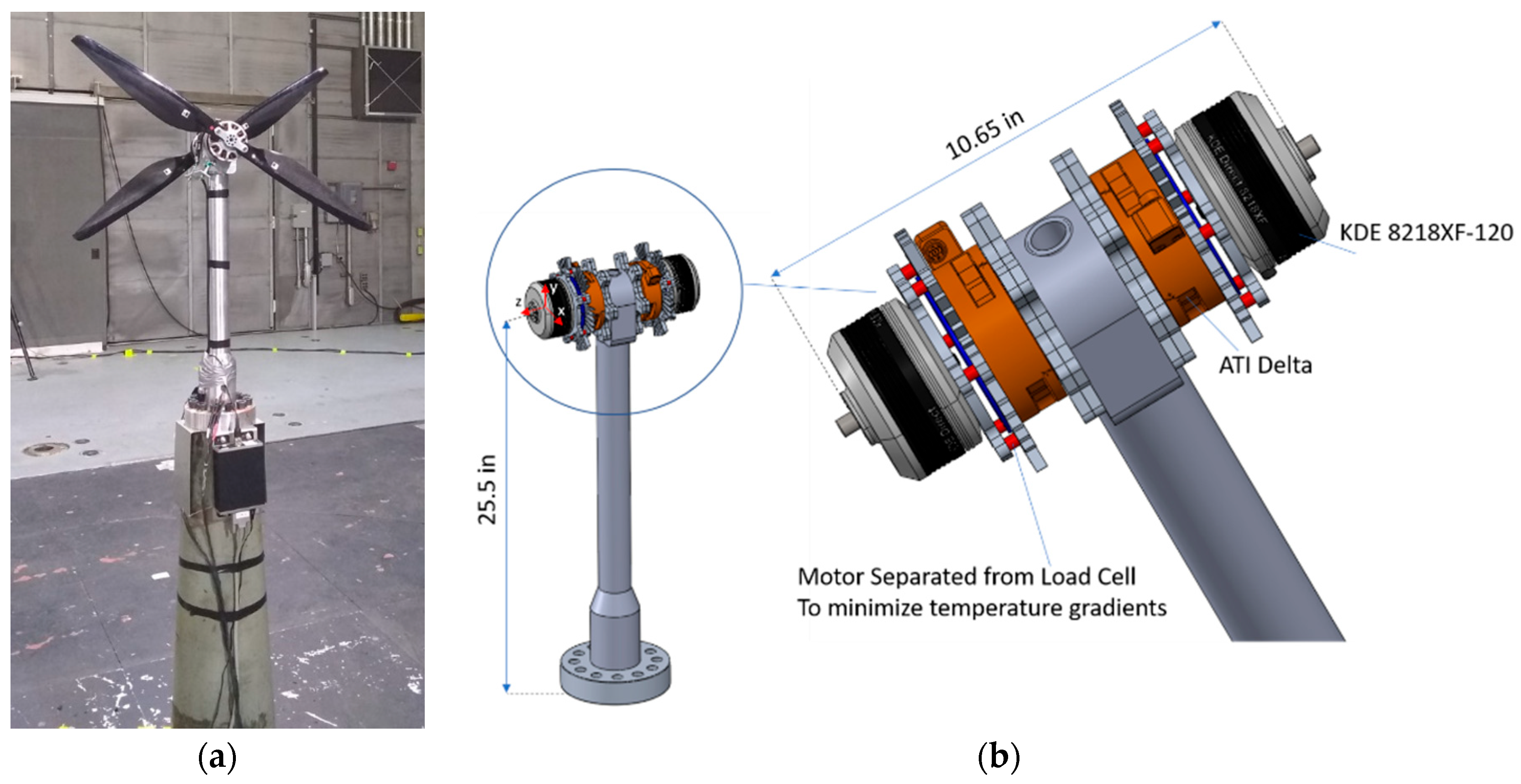
3. Experimental Test Setup

The experimental test setup of the coaxial rotor test stand is shown in the NASA Langley 14- by 22-ft. Subsonic Tunnel Facility in Figure 3 along with a schematic of the test stand. The motors (KDE8218XF-120) and rotors (KDE-CF305-DP, schematic in Figure 4) are commercial off-the-shelf products and were procured from KDE [82]. The method used to control the rotors with a pulse width modulation (PWM) signal is referred to as throttle control, which is reported by KDE on a percent scale from 0% to 100%. Each throttle position roughly corresponds to a specific RPM, but the resulting RPM can be slightly different based on a given wind-tunnel test condition and the instantaneous torque on the motors. The throttle settings used in the wind-tunnel test were 25, 50, 75, and 90%, which loosely correspond to about 1600, 2880, 3900, and 4515 RPM depending on the wind-tunnel test condition. Relevant parameters defining the basic coaxial rotor setup and operational conditions are included in Table 1.
ATI load cells [83] placed below each motor were used to record the three forces and three moments for each rotor versus time. Load cell range and resolution are reported in Table 2. The motors were instrumented with optical sensors to record blade phasing between the two rotors. The optical sensors also provided data to quantify the rotor RPM by calculating the fast Fourier Transform of the recorded square-wave time signal. All of the measurements were conducted at a sampling rate of 5 kHz, collecting 15,000 samples during each reading event. MATLAB R2021a was used to acquire the three forces and three moments for each rotor, blade passing signals, and load cell temperature signals. To obtain rotor performance values to compare with CFD, a moving average approach was used. A sensitivity study was conducted to determine the best size for the moving average calculation since the number of samples used in the moving average affects both the resulting thrust value and the associated standard deviation. One-quarter of a second, or 1250 samples, was chosen as a balance across all rotor speeds between obtaining low uncertainty from the moving averaging while still having several samples of the averaged data throughout the three-second time history to capture low-frequency variations due to unsteady flow conditions. This was incorporated into the experimental measurement uncertainty in Equation (5). The standard deviation dropped from 3.3 N at 50 samples to 0.5 N at 1250 samples. Post-processing of the data also revealed an increasing experimental uncertainty in descent conditions, with the maximum as high as 15%.

4. CFD Model Setup

This section details the CFD methodology developed from verifying the rotor geometry through the grid resolution studies, culminating in a resolution appropriate for a blade-modeled approach. Scanning of the KDE rotor will first be discussed along with comparisons with the CAD model provided by KDE. The discretization of the rotor blade into airfoil table stations, which must be precisely done to maximize the accuracy of the blade-modeled solution, will then be shown. Next, the process of generating the airfoil tables will be detailed. Finally, the RotCFD model rotor parameters, hub geometry, and grid refinement study will be discussed.

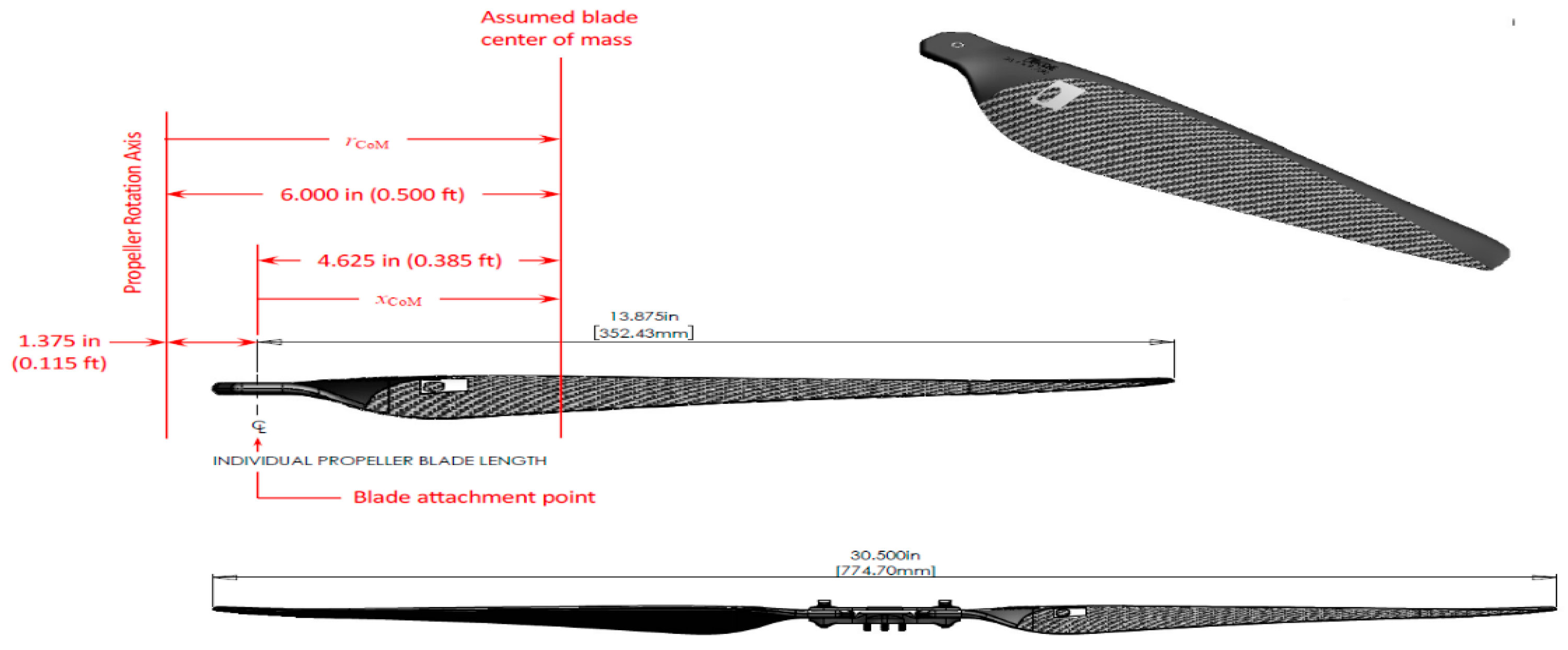
4.1. Rotor Geometry Verification

As previously mentioned, the experiment used two KDE 30.5” rotors. To verify the KDE-provided CAD geometry of the blades, both blades from a single rotor were scanned at JHU/APL using a Hexagon RS-6 laser scanner attached to an Absolute Arm 7-axis articulated arm. The arm and scanner combination provides a measurement resolution of 6 μm and an accuracy of 43 μm across the airfoil. The digital data obtained from the scan were used to create a point cloud that could then be compared to the original CAD model shown in Figure 5a below. The point cloud and CAD model were compared using 3D systems Geomagic Control X inspection software Version 2022.1.0. The Geomagic Control X output is a color map rendered from the airfoil showing the deviation in the measured hardware and the CAD file. An example of this color map for the lower surface of blade 1 is shown in Figure 5b. The deviations presented in Figure 5b range from zero shown in green to a maximum deviation of 0.9 mm shown in red. This was the maximum measured deviation for the rotor blades. Cross sectional comparisons of the CAD model and scanned geometry were also performed and further verified the accuracy of the manufactured blade. These comparisons are not shown here due to the proprietary nature of the KDE blade geometry. This gave confidence that the CAD model could be used to discretize the blade into appropriate airfoil tables based on the airfoil, Reynolds number, and Mach number distributions along the blade. This procedure is discussed in the following section.

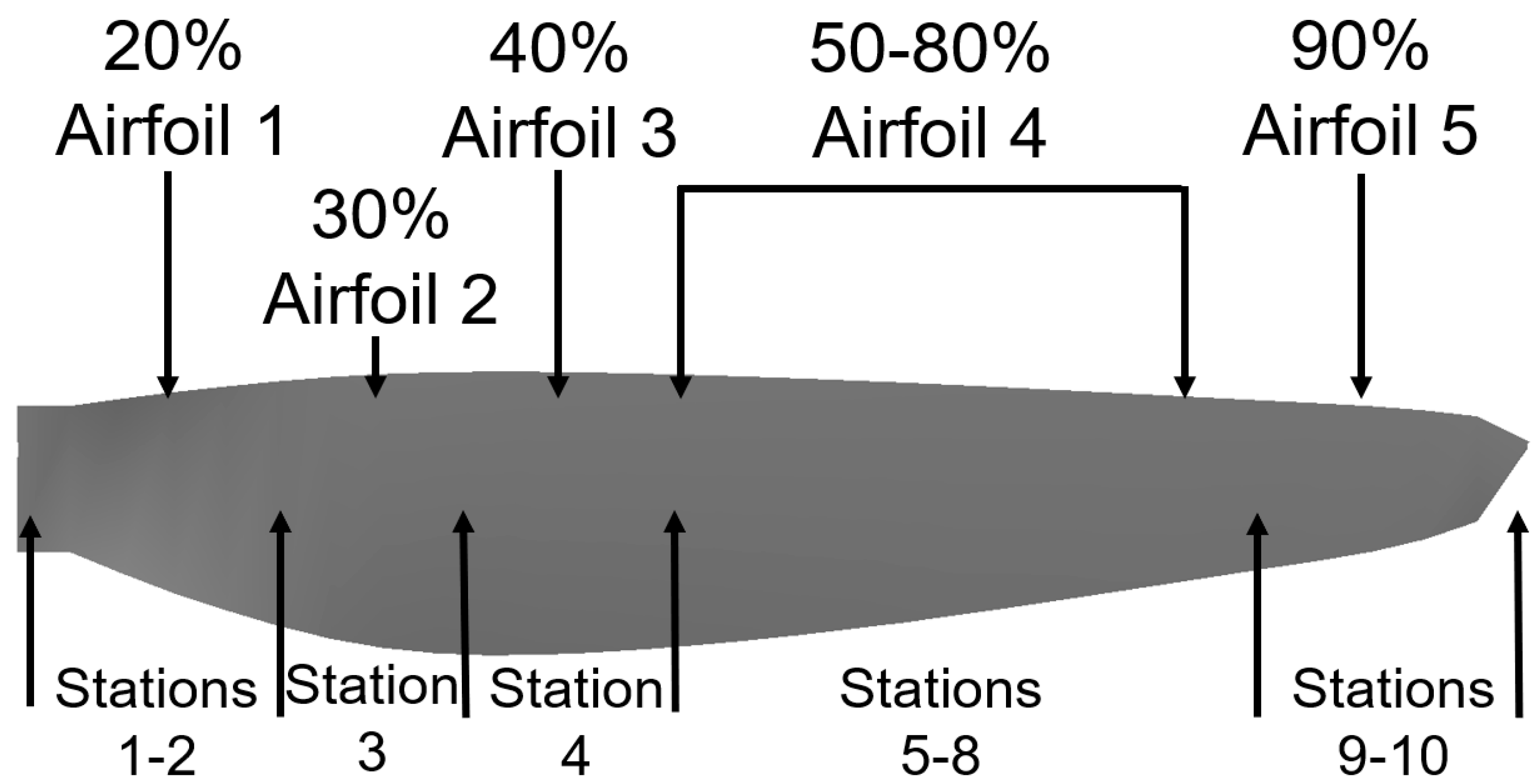
4.2. Blade Discretization into Radial Stations for the Airfoil Look-Up Tables

The next step after verifying the CAD model geometry was to discretize the blade into radial stations based on the airfoil distribution and the variation in Reynolds number and Mach number with the radial location, r/R, following the approach by Koning et al. [57]. The stations are used to generate C81 airfoil performance look-up table inputs used in RotCFD to calculate the momentum source strength at each location on the rotor disk. This step of discretizing the rotor blade into stations is essential due to the high variations in the blade performance radially. This variation is dependent on the local airfoil shape, the local Reynolds number, and the local Mach number.
Since the azimuthally and radially discretized rotor grid interface between the BEMT rotor model and the structured URANS solver has approximately 10,000 momentum source locations, the radial discretization of the C81 look-up tables is typically the coarsest part when compared to the cartesian grid or rotor grid. It is therefore advantageous to use as refined a blade discretization as possible to improve the accuracy of this blade-modeled approach. For small-scale rotors typical of UAM applications, such as the KDE rotor used in this study, the radial deviation in blade performance characteristics based on these factors can be quite significant. For example, the Reynolds number for this rotor ranges from below 100,000 near the root up to nearly 500,000 at the 75% radial location for the highest throttle setting used. The local Mach number range covers from less than 0.1 up to as high as 0.55. Although the blade tip Mach number can reach as high as 0.55, the inflow and wake velocities in the URANS flowfield remain below a Mach number of 0.25, and thus, the simulation is solved using the incompressible URANS equations. The ARC2D two-dimensional airfoil CFD look-up tables used in the calculation of momentum sources for the rotors, however, do capture compressibility effects and show notably different characteristics at different operating points within these Mach and Reynolds number ranges, which is discussed further in Section 4.3. This means that compressibility effects of high Mach flow over the rotor blade are accurately accounted for.
The discretization is shown below in Figure 6 and includes a total of ten radial stations. Blade cross sections were analyzed every 6.35 mm (0.25 in) to identify the blade’s airfoils. Five different airfoils were identified and are labeled with approximate locations in the figure. Radial stations using the same airfoil are grouped together to increase figure legibility but are still separate in practice to account for the radially varying Mach and Reynolds numbers even for the same airfoil section.

4.3. C81 Airfoil Table Generation

Following the discretization of the rotor blade into ten radial stations, an airfoil performance table was generated for each station. A two-dimensional compressible CFD solver, C81 Generator, was used for this step. The C81 program is a wrapper for the two-dimensional thin-layer Reynolds Averaged Navier–Stokes CFD solver, ARC2D, which was developed by the U.S. Army’s Rotorcraft Group and is currently supported by Sukra Helitek, Inc., Ames, IA, USA [84]. The C81 Generator program contains the entire workflow from airfoil specification, or airfoil geometry import, through to the analysis and exportation of the airfoil performance versus the angle of attack as a function of the Reynolds number and Mach number.
The program was run as fully turbulent using an algebraic mixing length turbulence model along with a thin-layer approximation for turbulent flows [85]. The Reynolds number ranges analyzed in this paper would not typically be considered fully turbulent and the resulting impact of this assumption must be carefully assessed. Several factors indicate that this particular rotor configuration is likely to have near fully turbulent rotor blade operation, including the chaotic flowfield of two rotors operating in close proximity to each other. Several other factors causing laminar to turbulent transition are also suspected here.
The uncertainty associated with this fully turbulent vs. free-transition airfoil performance assumption, which corresponds to the input uncertainty from Equation (4) as described in Section 2.4, was found by comparing the results from identical simulations with the exception that one set used the aforementioned fully turbulent C81 tables, while the second set used lower-order free-transition airfoil tables. These free-transition airfoil tables were generated using the MIT-XFOIL tool [86]. A second set of free-transition airfoil tables was also created with the MIT-MSES multielement airfoil design and analysis system that predicts airfoil lift and drag coefficients through solving the Euler equations [87] to build confidence in the lower-order free-transition airfoil performance data. An example of lift curve slopes for the fully turbulent vs. free-transition airfoil performance data is included in Figure 7.
The results from flight conditions such as climb, forward flight, and descent were compared. The maximum uncertainty values were calculated for the various rotor performance metrics as the percentage difference between the fully turbulent and free-transition results, and are summarized below in Table 3. Although the airfoil drag coefficient increases sharply with a fully turbulent assumption, the input uncertainty in the predicted torque is small since the profile power, which is the portion affected by a drag coefficient increase, is roughly one-fifth of this rotor’s total power. The observed decrease in thrust also reduces the rotor-induced power, so the predicted torque is almost unaffected by the fully turbulent vs. free-transition assumption.
The best practices of C81 table creation will now be briefly described. A structured airfoil-fitted O-grid was chosen for this study to best model a blunt trailing-edge airfoil, which was a good representation of the manufactured blade. The airfoil grid can be seen in Figure 8a. The blunt trailing edge has two distinct corners, as depicted in Figure 8b. A grid refinement study was carried out following the procedure specified by Koning [57,58] to determine the appropriate number of periodic and normal cells. The simulation was run with 301 wrap-around points on the airfoil (i.e., 150 cells on both the upper and lower surface), 201 normal points, and 20 cells covering the blunt trailing edge, or the space between the upper and lower surface. Comparisons were made for completeness between this blunt trailing-edge grid and one with a rounded trailing edge, which is another choice when using the program’s O-grid. The rounded trailing edge required three times the number of total cells to reach grid refinement convergence and resulted in airfoil performance similar to the blunt trailing-edge grid, so the blunt trailing-edge grid was used. The solver automatically switches to a time-accurate approach if convergence has not been reached in a specified number of steps, if periodicity is detected in the output, or if the absolute value of the angle of attack is greater than ten degrees.
The C81 Generator simulations were run from an angle of attack from −20 to +20 degrees. Outside this range, the airfoil tables use NACA 0012 experimental data at the appropriate Reynolds number as an approximation of airfoil performance beyond stall, where the airfoil performs practically as a flat plate [88]. Blending the airfoil performance parameters from the C81 data with the 0012 data was carried out using the Viterna–Corrigan correction, which is based on an empirical approach for extrapolating post-stall sectional airfoil performance based on the flat-plate theory and the rotor dimensions [89,90]. An example of the sectional lift coefficient and drag coefficient versus angle of attack can be seen in Figure 9.
The plots are again generically referenced in deference to the proprietary KDE rotor information. Accurately modeling the airfoil performance at the extreme values of around +/−180 degrees is important for capturing the proper aerodynamics in the reversed-flow region of the non-articulated rotor in edgewise flight. The simulation results rely heavily on these airfoil performance input decks, so careful consideration was used to create them and ensure a realistic representation of the airfoil performance across all possible conditions.
Although the sample C81 data in Figure 9 only represent a single Reynolds number and Mach number combination, each station was run at four combinations of Reynolds number and Mach number to account for the operational range of RPMs that was used in the experimental testing. The effects on the lift and drag coefficients that are observed with changing Mach number and Reynolds number for a given airfoil can be observed in Figure 10.

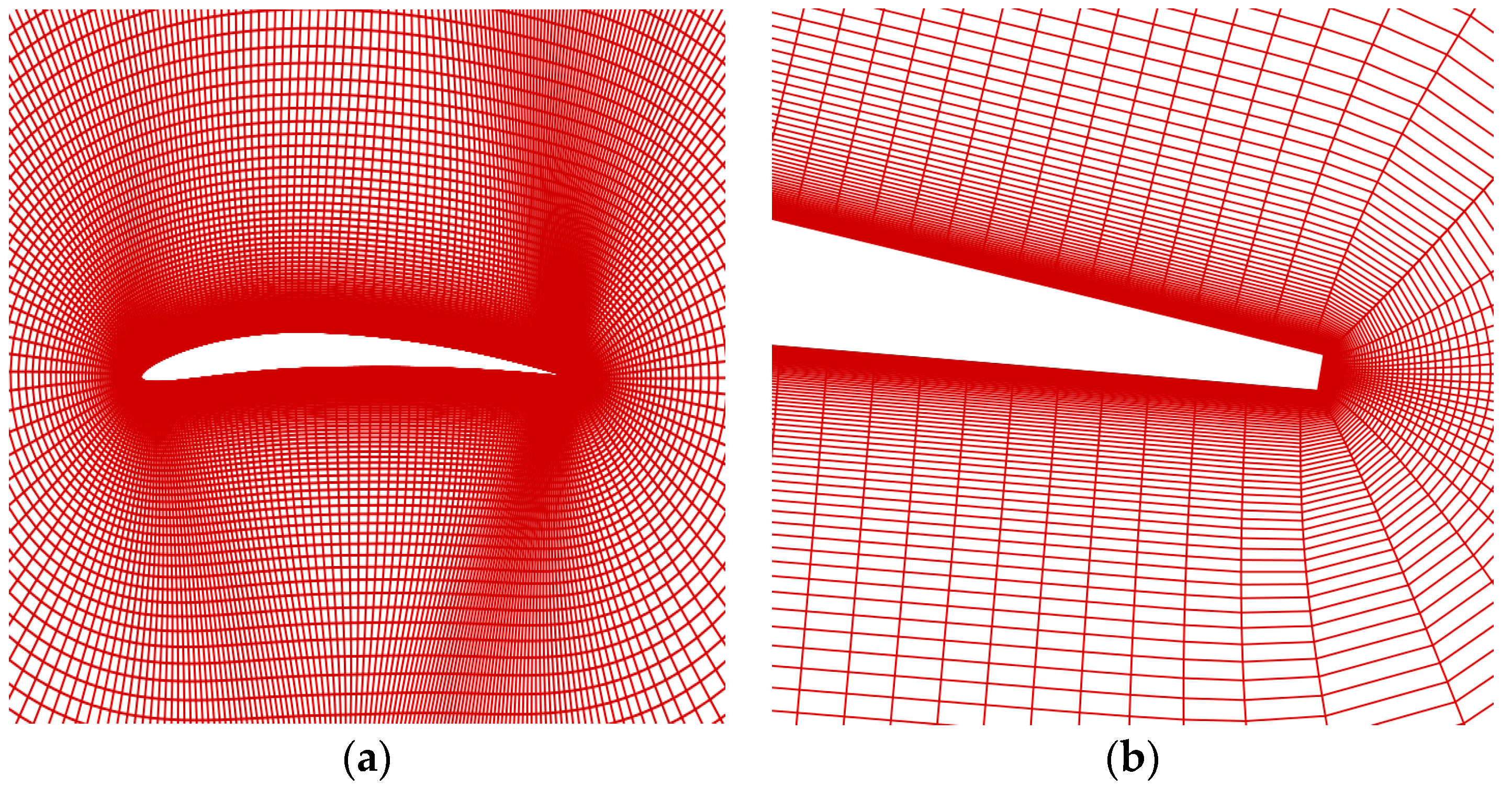
4.4. RotCFD Model Creation

Hub geometry for the RotCFD model was created in SolidWorks and was meant to accurately capture the shape of the hub, motors, load cells, and sting mount. A sensitivity study was carried out to determine the effects of hub geometry fidelity, and the rotor performance results were found to be insensitive to fine details in the geometry. A representative geometry was thus used that captures the general shapes and contours of the assembly for blockage effects. This geometry was combined with the rotor models to create the full model. The chord and twist distributions obtained from the rotor CAD model, as well as the C81 tables that have already been discussed, were added as inputs to finish the rotor model. Front and side views of the RotCFD model are shown in Figure 11a and Figure 11b, respectively.
The near-body flowfield grid, from the view that will be used for flow visualizations in this work, is shown in Figure 11c. The included rotors are for illustration purposes only. RotCFD uses body-fitted tetrahedral cells to conform the grid to the hub geometry, as can be seen in the figure. The far-field boundary is located 20 rotor diameters away from the model. Grid refinement studies were carried out to determine the grid resolution required to minimize the discretization uncertainty in the CFD result. The highest refinement level is held constant throughout the region including the rotors and hub geometry, which maintains a consistent grid for rotor–rotor interaction and interference with the hub geometry. This refinement region extends beyond the rotors far enough to ensure smooth pressure contours at the junction between this highest refinement level and the subsequent one. Increasing the final grid cell count by 250% resulted in changes of less than 1% in hover to the upper rotor thrust and power and the lower rotor thrust. The change in lower rotor power was the largest at 2.6% in hover. At an advance ratio of 0.06 relative to the wind-tunnel forward-flight testing, the changes in the upper rotor were again below 1%, and the lower rotor thrust and power were within 3.25% for the grid used compared to the further refined one.
These values represent the numerical uncertainty from Equation (4) for the upper and lower rotors, and the maximum values from the hover and forward flight studies are summarized in Table 4. The changes to the lower rotor performance with cell count increase are likely due to the higher resolution tracking of the upper rotor wake contraction into the lower rotor. The authors accepted that this CFD uncertainty would have a lower simulation time that would be manageable for running the several hundred cases required for the coaxial rotor performance matrix. The final model grid has approximately 350,000 cells, which is two to three orders of magnitude less than those of conventional blade-resolved CFD. This is one of the greatest advantages of the hybrid BEMT URANS methodology: the flow physics relevant for steady rotor performance predictions can be accurately modeled without resolving the boundary layer aerodynamics, as is done in conventional blade-resolved CFD. As stated previously, this large reduction in grid cell count allows for massive parallelization of the modeling approach on GPU-accelerated machines, resulting in several orders of magnitude speed increases.

5. Results

The results are presented first with a discussion of the experimental data. Comparisons are then made between experimental data and the CFD predictions, along with conclusions being drawn from those comparisons. Finally, a section covering the results from the descent is presented.

5.1. Discussion of the Experimental Data

The experimental data were measured at 5 kHz. The measured time histories have large fluctuations that were due to various factors including rotor–rotor interaction, test stand vibrations, and unsteady flow conditions. To obtain rotor performance values to compare with those of CFD, a moving average approach was used. A sensitivity study was conducted to determine the best size for the moving average calculation since the number of samples used in the moving average affects both the resulting thrust value and the associated standard deviation. One-quarter of second, or 1250 samples, was chosen as a balance across all rotor speeds between obtaining low uncertainty from the moving averaging while still having several samples of the averaged data throughout the three-second time history to capture low-frequency variations due to unsteady flow conditions. This was incorporated into the experimental measurement uncertainty from Equation (5). The standard deviation dropped from 3.3 N at 50 samples to 0.5 N at 1250 samples; a sample size of 50 represents 0.65 revolutions at the 75% throttle setting, while 1250 samples represent 16 revolutions. The averaged thrust value was relatively insensitive to the number of samples, but the standard deviation dropped rapidly from an initially high value. Post-processing of the data also revealed an increasing experimental uncertainty in descent conditions, with the maximum as high as 15%.

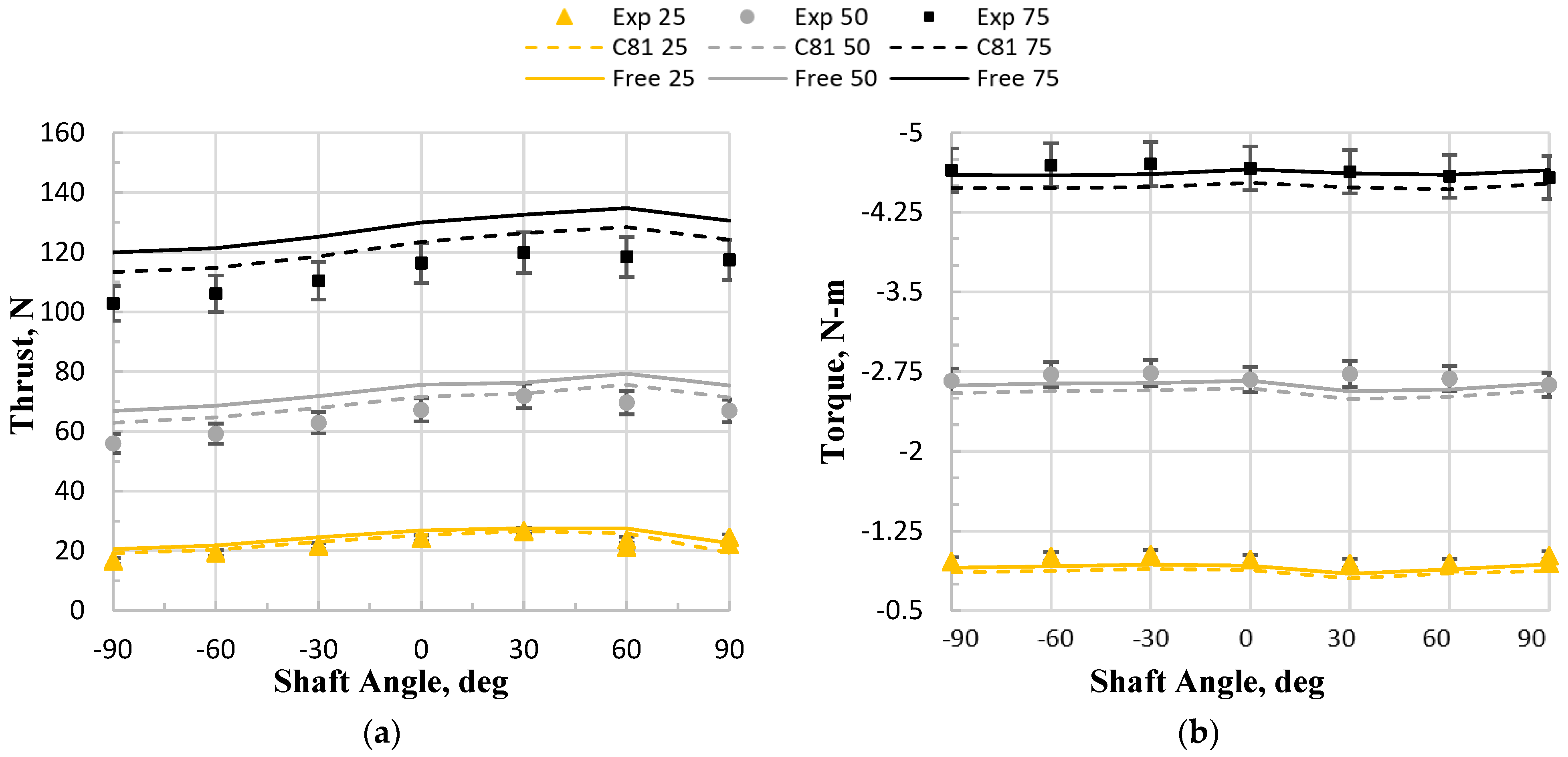
5.2. Comparison of the Experimental Data to RotCFD Predictions

After the rotor thrust and torque were post-processed, they were overlaid with the CFD results as a function of both rotor shaft angle and throttle setting. Shaft angle, SA, is defined as the angle between the free-stream wind-tunnel velocity and the coaxial rotor system’s tip-path plane. In Figure 12, a red dot is placed on the upper rotor of the coaxial configuration. For single rotor experimental runs and CFD simulations, the lower rotor was removed.

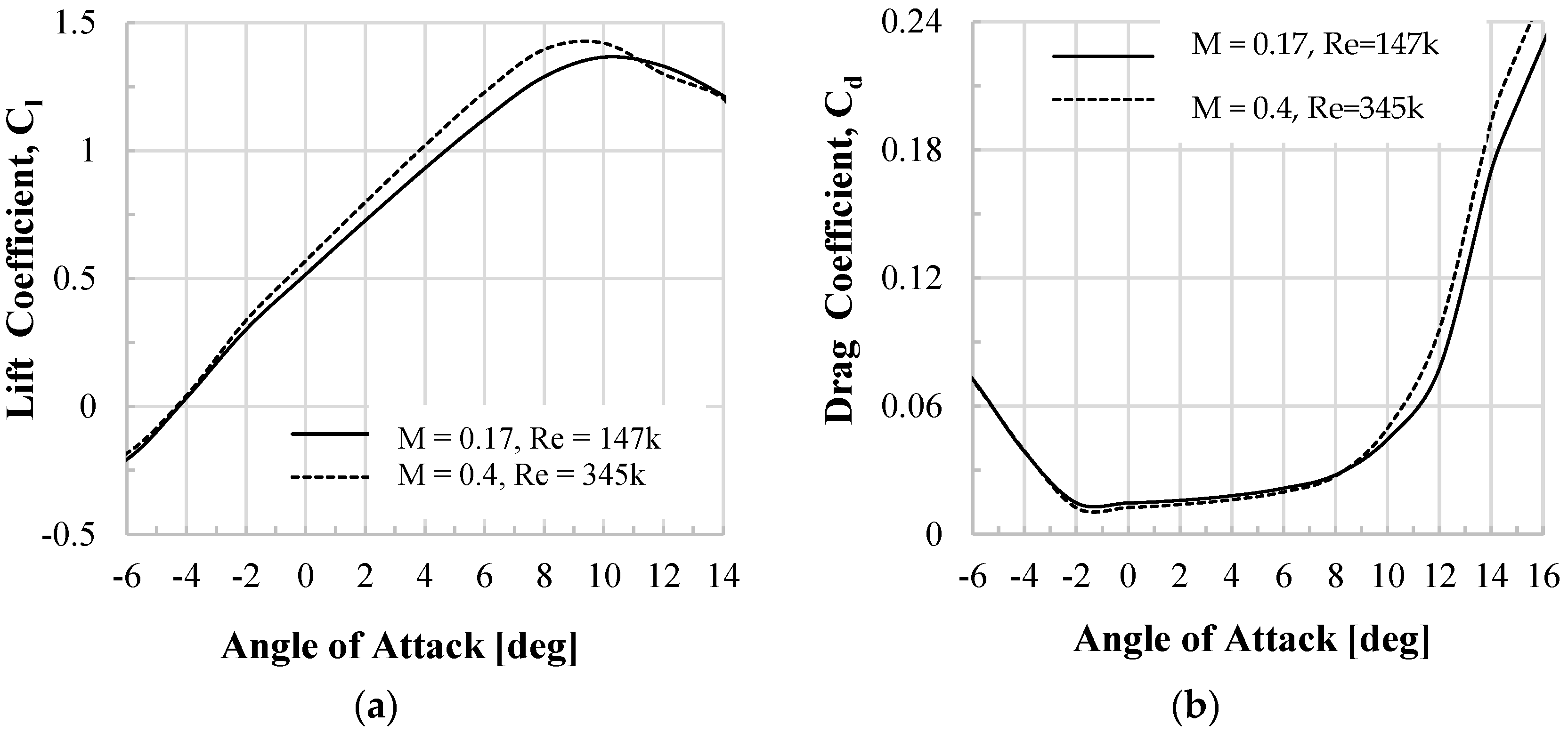
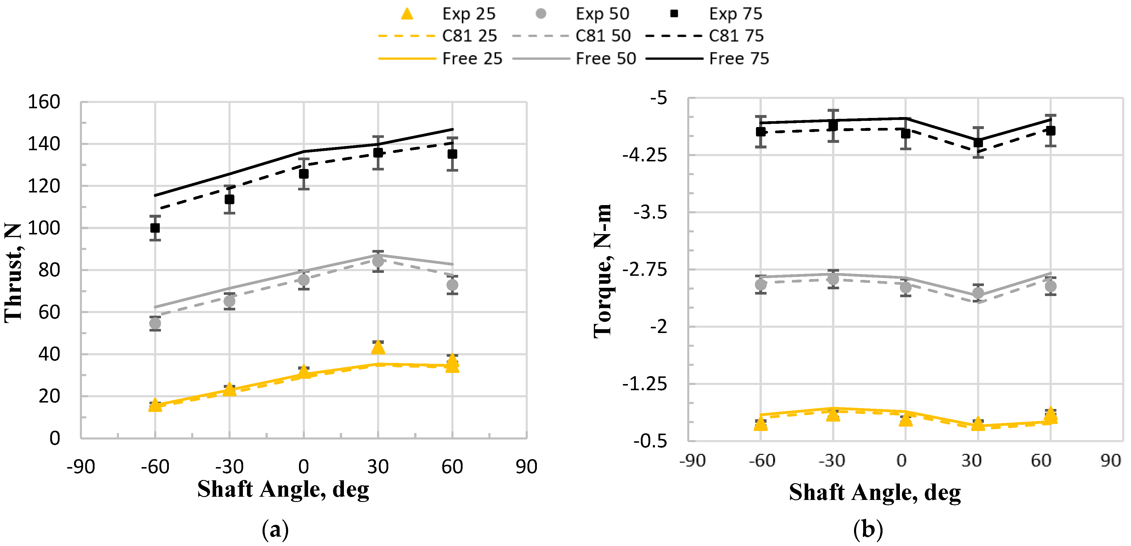
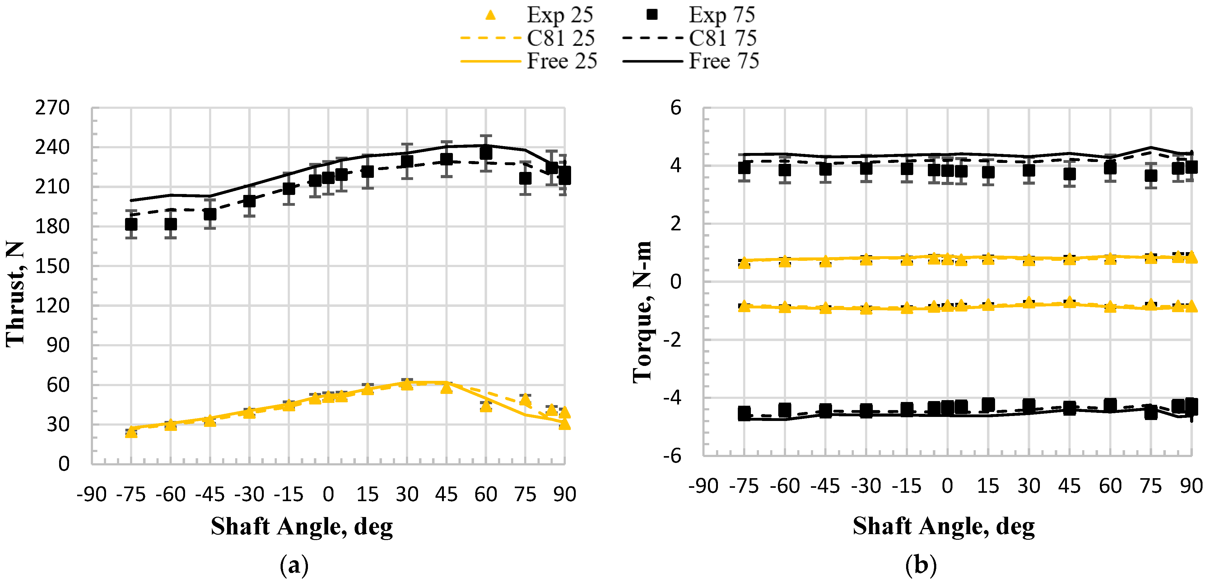
5.2.1. Single Rotor: Free-Transition vs. Fully Turbulent Airfoil Tables

The results are first presented comparing the single rotor performance of the experimental data with both the free-transition and fully turbulent airfoil performance assumptions. Figure 13 depicts the single rotor thrust and torque comparisons for a wind-tunnel velocity of 3.81 m/s over the full range of shaft angles. Three throttle conditions are included on each chart, which are the 25%, 50%, and 75% throttle settings that loosely correspond to about 1600, 2880, and 3900 RPM depending on the wind-tunnel condition. The charts compare the experimental data to the CFD results using either a free-transition ‘Free’ or fully turbulent ‘C81’ assumption of airfoil performance.
Figure 14 plots the same information, but for 7.62 m/s. The charts represent 36 experimental test conditions and 72 CFD simulations of the single rotor configuration. For most cases, the fully turbulent airfoil performance tables provide better correlation with the experimental thrust data. The results for the torque comparisons are less consistent in terms of a trend, which indicates that the impact on torque of the decreased drag coefficient for the free-transition airfoil tables is negated by the increase in rotor thrust associated with the steeper lift curve slope. Since thrust is thus the more sensitive parameter, the fully turbulent C81 airfoil performance tables are deemed the better fit to the experimental data and the better representation of the flow physics. This result could be counter-intuitive since the low Reynolds numbers would suggest some portion of the airfoil chord to be experiencing laminar flow. The complex flow conditions, however, of this small-scale, high tip-speed rotor system could be responsible for early transition and one explanation as to why the fully turbulent airfoil performance tables correlate better with the experimental data than the free-transition tables do.
Of special note when viewing these charts is that the experimental uncertainty values increase when moving to the higher shaft angles, which are representative of descent conditions. The primary conclusion is that the complex flowfields of the vortex ring state (VRS), turbulent wake state (TWS), and windmill brake state (WBS) create challenging test conditions in the wind tunnel. Still, the average deltas are within 4% for both thrust and torque. Table 5 further summarizes the deltas of the simulations of the experimental data by flight condition. For the C81 fully turbulent airfoil tables, climb conditions have the largest thrust discrepancy at 6% (over-predicted) and the descent conditions have the largest torque discrepancies at −5.5% (under-predicted). The average torque delta of the free-transition model is lower, but the corresponding average thrust delta is much higher at 9.5%. In this work, thrust is typically deemed the more important parameter for reducing prediction uncertainty, so the C81 fully turbulent tables are again identified as the better fit to the data.

5.2.2. Coaxial Rotor: Free-Transition vs. Fully Turbulent Airfoil Tables

This section begins with a similar analysis comparing rotor performance predictions of the coaxial rotor system with experimental data when using free-transition versus fully turbulent airfoil tables. Simulation results are then presented in the subsequent section comparing rotor performance predictions of the single rotor model to both the upper and lower rotors of the coaxial model versus shaft angle.
A similar analysis comparing the CFD rotor performance predictions using both free-transition and fully turbulent airfoil tables to the experimental data was conducted. The results are reported in Figure 15a for the combined coaxial rotor thrust. The upper and lower rotor torques are compared separately in Figure 15b, where the upper rotor torque values are negative and the lower rotor torque values are positive due to the sign convention of the rotation directions. These data for the coaxial rotor system are at a wind-tunnel velocity of 6.1 m/s, compared to the single rotor cases at 3.81 and 7.62 m/s. Only simulations of the 25% and 75% throttle conditions were completed and are plotted in the figure against the corresponding experimental data.
The trends of the free-transition versus fully turbulent simulations are the same as for the single rotor cases. The free-transition airfoil performance tables still have the same higher lift curve slopes, which results in a higher thrust coefficient and thrust value when all other settings are held constant. This is explained by the relationship between thrust coefficient and average rotor lift coefficient. Of special interest in Figure 15a is the reversal of the trends for ‘C81 25’ versus ‘Free 25’ in a high rate of descent, i.e., for shaft angles between 45 and 90 degrees. At the low Reynolds numbers associated with this rotor, the fully turbulent airfoil performance keeps the boundary layer attached to the airfoil until higher angles of attack are reached, as compared to the free-transition performance. This combination of low rotor speed and a high rate of descent along with the observed reversal in the trend of predicted thrust indicates that the lower rotor is approaching stall in this region, and thus, the free-transition airfoil tables would have a lower airfoil lift coefficient.
Comparisons of predicted torque with the experimental data were also made. The trends were consistent with the single rotor analyses in that the free-transition simulations predict an overall higher magnitude of rotor torque. Again, this is because the free-transition simulations are producing more thrust (except for beyond stall in high shaft-angle descent conditions), which results in higher induced power (hence torque) and drives the result. The torque predictions for all simulations are over-predicted, with the fully turbulent predictions consistently providing a better correlation with the experimental data.
The coaxial rotor thrust comparisons are summarized in Table 6. The average coaxial rotor thrust delta is 1.4% across all conditions for the fully turbulent simulations, which is in line with the single rotor results. The coaxial rotor power is also in better agreement with the fully turbulent simulations, which confirms the C81 model with the fully turbulent airfoil performance assumption as the better fit.
Returning to the uncertainty analysis discussed in Section 2.4, the experimental uncertainty for various flight conditions is reported in Table 7. The lower rotor thrust has the highest experimental uncertainty at 14.7% for descent conditions.
The test program had several descent cases to capture the unsteady rotor behavior in these conditions, and as such, the deltas from that segment dominate the average deltas reported across all flight conditions. The calculated experimental uncertainties often have some minimum value, which is set by the repeatability uncertainty within the experimental uncertainty root sum of squares calculation. The repeatability uncertainty for each metric was generated by averaging the discrepancies across all of the 25% throttle repeat points. This single averaged value was used as the repeatability uncertainty across all of the respective cases and was the driver of the total experimental uncertainty. It was discovered that using this low thrust and torque condition, i.e., 25% throttle, for the repeat runs led to the absolute magnitude of the experimental errors being a larger total percentage of the measured values. It would be beneficial to use a higher throttle setting for this repeatability measurement in the future, such as the 75% throttle condition, to decrease the percentage repeatability uncertainty and thus the total experimental uncertainty. Alternatively, multiple repeat data points could be obtained to characterize the repeatability uncertainty separately for each throttle setting and for different portions of the test matrix, such as forward flight, climb, and descent.

5.2.3. Single vs. Coaxial Rotor: Fully Turbulent Airfoil Tables

Since the previously reported single rotor and coaxial rotor test conditions were not acquired at the same wind-tunnel speeds, the results are best as non-dimensionalized using the rotor thrust coefficient equation defined in the nomenclature to compare between the two configurations. Within each wind-tunnel sweep and throttle grouping, the method of controlling rotor speed with throttle also leads to some deviation in the rotor RPM as a function of the wind-tunnel test condition. Non-dimensionalizing the thrust coefficients helps to remove these discrepancies. Here, the comparisons are shown as a function of shaft angle to highlight the differences based on flight condition, i.e., climb, edgewise flight, and descent.
The predicted single and coaxial rotor thrust coefficients at the 75% throttle setting are plotted in Figure 16a as a function of shaft angle. The same data at the 25% throttle setting are included in Figure 16b. The predictions are from the RotCFD models using the fully turbulent airfoil performance tables, which are used for the remainder of this discussion. The single rotor data (dashed light-gray line) are simulations of both the upper rotor removed and the lower rotor removed. These single rotor performance predictions differ slightly from one another due to the interaction of the sting arm being either ahead of or behind the rotor. Of special interest is that the single rotor data closely approximate the upper rotor performance of the coaxial rotor system. This is very apparent in Figure 16a for forward-flight conditions (SA = −30 to 0 deg) where the rotor–rotor interaction is small and the upper rotor in the coaxial configuration mostly encounters undisturbed inflow. For steep climb conditions (SA = −90 to −45 deg), the single rotor predicted thrust coefficient is a bit higher than that of the coaxial upper rotor. This is likely due to the fact that in a climb condition, the wake skew angle is small and the rotor–rotor interaction is high. Thus, the upper rotor in these conditions is affected by the presence of the lower rotor.
What is more interesting, however, is this comparison for other flight conditions such as descent, which corresponds to shaft angles of +5 deg and greater, with axial descent at +90 deg. Depending on the throttle setting and flight speed, the lower rotor can exhibit blockage effects on the upper rotor and lead to large rotor–rotor interactions that affect each rotor’s performance. For the 75% throttle condition shown in Figure 16a, however, the ratio of induced velocity to flight speed is large enough that even the descent conditions do not cause abrupt shifts in the thrust coefficient. For this case, the single rotor performance is still a good predictor of the coaxial rotor’s upper rotor performance even in descent conditions.
The lower induced velocity of the 25% throttle condition at the same wind-tunnel speeds results in the rotor performance being affected much more by the oncoming wind-tunnel flow. The degree to which the flow affects the rotor performance is a function of the rotor shaft angle, which determines the individual rotor wake skew angle and the magnitude of the wind-tunnel flow velocity normal to the rotor disk. In climb conditions (SA= −90 to −30 deg), the flow normal to the rotor disk acts to reduce the thrust coefficient for all cases. For forward-flight and edgewise cases (SA = −25 to 0 deg), the oncoming wind-tunnel velocity clears the upper rotor wake from the lower rotor, i.e., a large wake skew angle. This results in minimal rotor–rotor interaction and all three rotors having similar behavior. As descent conditions are approached (SA = +15 to +45 deg), the single and coaxial rotor systems are affected by VRS conditions in two very different ways.
VRS is a known phenomenon that is well documented for rotorcrafts by Leishman et al., Johnson, Brand et al., and Brown [91,92,93,94]. Coaxial rotor systems, however, have been studied much less in VRS conditions. Cornelius et al. and Kinzel et al. [29,50] documented some computational findings from a coaxial rotor system in and around VRS. The conclusion was that a coaxial rotor system may benefit from a sort of ‘VRS shielding’ as the lower rotor delays the upper rotor’s loss of thrust to a higher descent speed. This is observed again in this work and confirms prior findings.
Of special note is that the lower rotor in Figure 16b is highly affected by VRS conditions, while the upper rotor’s VRS effects are delayed until a higher shaft angle is reached, which can be thought of as a higher rate of descent if considering flow normal to the rotor disk. The VRS effects on the coaxial lower rotor are noticed in the very early stages of descent, at which point the slope of the thrust coefficient vs. shaft angle reverses direction when the descent rate becomes high enough to entrain the wake. At still higher shaft angles approaching axial descent (SA = 60 to 90 deg), the lower rotor thrust coefficient begins again trending upward, signifying a cross over into the turbulent wake state and stalled rotor performance. These observations are also in agreement with the experimental uncertainties, which increase in the descent conditions due to the unsteadiness of VRS-type conditions.
For the 25% throttle condition, the single rotor performance initially tracks closely with the upper rotor of the coaxial configuration. At higher shaft angles, however, the two start to differ. For this combination of wind-tunnel velocity and throttle setting, the single rotor achieves a higher thrust coefficient in the early stages of descent (SA = 0 to +30 deg), which can be attributed to the fact that there is no lower rotor shielding it from the oncoming flow. As the shaft angle increases, which can be thought of as higher rates of descent for a fixed speed, the thrust coefficient changes trend at +30 deg. This indicates the onset of the VRS effects at a lower shaft angle, or a lower rate of descent, as compared to the upper rotor of the coaxial configuration with a notable change in trend at +60 deg.

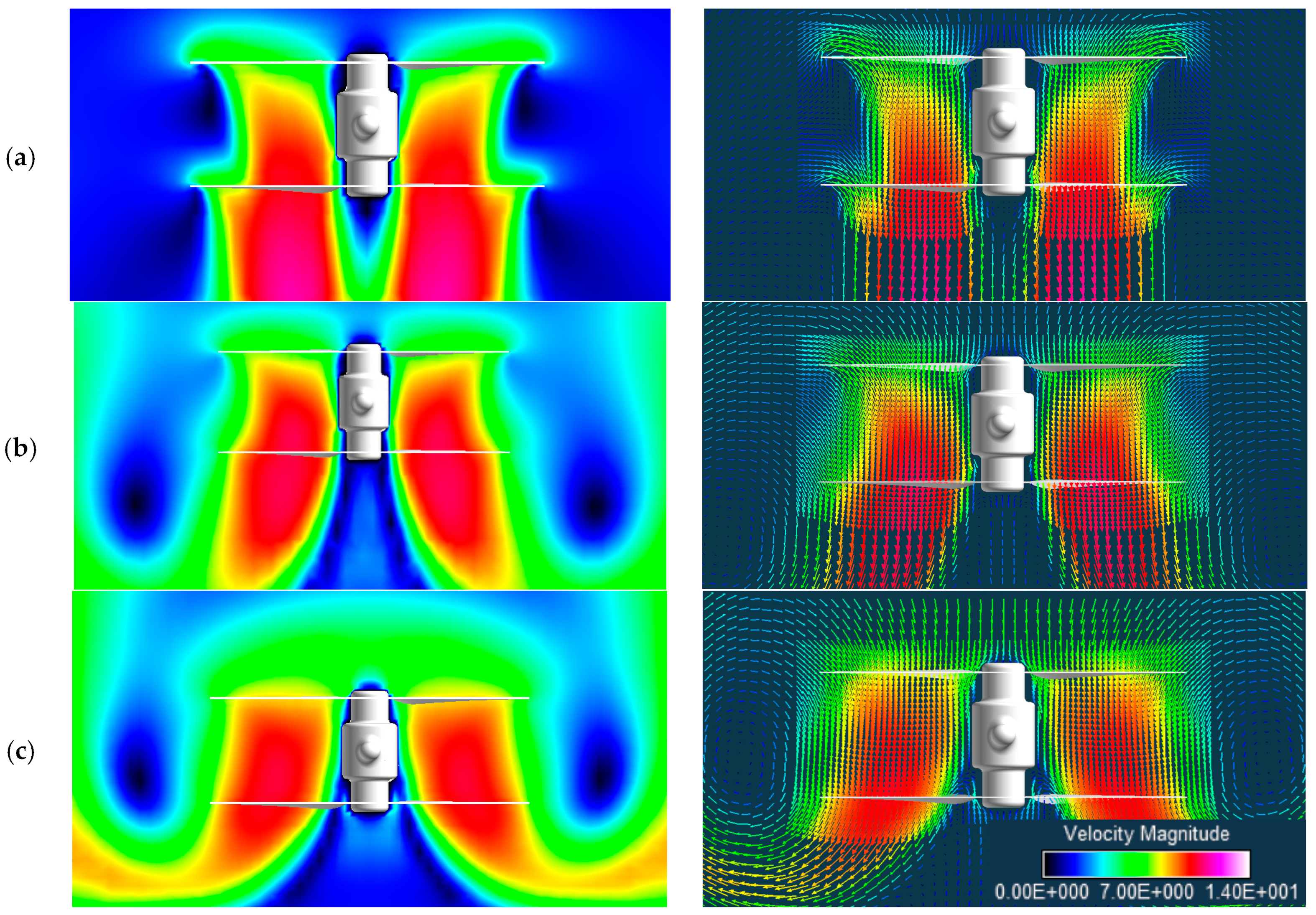
5.3. Axial Descent and Continued Discussion on the Vortex Ring State

To explore this ‘VRS shielding’ phenomenon more deeply, the coaxial rotor system was simulated at various rates of descent. Taking a closer look at the CFD results in this region can highlight the effects being observed. Figure 17 includes disk plots of the coaxial rotor system’s lift coefficient for the upper and lower disks in axial descent, which corresponds to a shaft angle of 90 degrees. The figure includes three descent speeds. Lift coefficient values too high suggest rotor stall and values too low suggest poor performance. A mostly normal operating condition can be seen in the disk plots from the 2.29 m/s descent, in Figure 17a, with a reasonable lift coefficient in all places except for the upper rotor root region that appears to be stalled. The upper rotor blade tips also appear to be approaching high lift coefficient values. The area where the upper rotor wake passes through the lower rotor does also exhibit some reduction in the lower rotor lift coefficient. The 4.57 m/s descent condition, in Figure 17b, sees an even larger depletion of lower rotor thrust, indicating highly decreased performance. The upper rotor appears to be performing adequately, but it is important to note that the lift coefficient has been decreased following an increase in descent rate. These two observations suggest the formation of a toroidal vortex ring in the vicinity of the coaxial rotor system. This will be highlighted momentarily in Figure 18. The upper rotor, however, is still operating at a reasonable lift coefficient despite the higher descent rate that could otherwise be expected to push the rotor toward stalling. The highest descent velocity of 6.1 m/s, in Figure 17c, shows complete degradation of the values across both the upper and lower rotors. The lower rotor’s root section is seen to be stalled with the high descent velocity, yet the outboard sections have low values due to the surrounding toroidal vortex ring. The mid-section of the lower rotor is seen to have a higher average lift coefficient than the previous condition, indicating that the vortex ring is translating higher on the coaxial rotor system and the lower rotor is being exposed to more of the oncoming flow from the descent velocity. This condition is beginning to transition from a VRS to a turbulent wake state.
To better visualize this phenomenon, the vortex rings are highlighted in Figure 18 with plots of velocity magnitude and velocity vectors for the same three conditions. The 4.57 m/s descent plots have a toroidal wake structure just beneath the lower rotor plane that acts to increase the inflow through the lower rotor and decrease its sectional values, but it is kept at a distance from the upper rotor. This is indicative of the observed ‘VRS shielding.’ The bottom plots of Figure 18, representing the higher descent speed, show that the vortex ring has moved up and is now encompassing the entire coaxial rotor system. The location of the toroidal vortex ring can be identified by the low velocity region at the core of the vortex ring, which is located just beyond the rotor blade tips in Figure 18b,c. This represents a fully developed coaxial rotor VRS that is approaching a transition to a turbulent wake state.
The results of Figure 17 and Figure 18 corroborate the trends observed and described from the performance comparisons. In Figure 16a, both the upper and lower rotor thrust coefficients increase as the rotor system transitions from axial climb (−90 deg) to edgewise flight (0 deg), and finally to axial descent (90 deg). This is indicative of normal operation, which is expected at low velocity relative to the inflow speed. Figure 16b, with the decreased rotor speed, shows a similar trend at first where the individual rotor thrust coefficient increases from the climb, through edgewise flight, and into the descent. An inflection point is observed on the lower rotor, however, at the start of descent conditions. At this point, the lower rotor is beginning to entrain its wake, and the thrust coefficient is observed to continually decrease as the condition approaches axial descent and the vortex ring centers around the lower rotor. The upper rotor sees a delayed inflection point and less of a drop in thrust coefficient, which again agrees with the proposed VRS shielding theory. For the highest rates of descent, shown in the right portion of Figure 16b, both the upper and lower rotor thrust coefficients exhibit similar behavior as the vortex ring moves higher in the rotor system. Still, the upper rotor exhibits a more gradual entrance into the VRS region with a smaller total drop off as well.

6. Conclusions

This paper presented a methodology for accurate and efficient multirotor performance estimation using a hybrid BEMT-URANS CFD approach. The accuracy of the methodology was quantified using experimental test data obtained by the authors in the NASA Langley 14- by 22-ft. Subsonic Tunnel Facility. The computational efficiency of the approach was also discussed with some mention of the computational hardware, GPU acceleration, and runtimes achieved through optimized scripting of the simulations on a multi-GPU desktop machine. These data characterize the approach as retaining a high level of accuracy for predicting steady multirotor performance while greatly reducing the computational cost to be several orders of magnitude less than that of high-fidelity CFD. Additionally, this paper presented an analysis of single versus coaxial rotor performance. Insights were provided into the ‘VRS shielding’ phenomenon unique to the coaxial rotor system that is observed to delay the full effects of VRS until higher descent speeds are reached.
The objectives of this work were as follows:
  • Summarize a methodology for multirotor performance prediction using an efficient hybrid BEMT-URANS CFD approach with a high-resolution model of the rotor.
  • Document the effects of using fully turbulent versus free-transition airfoil performance tables on CFD rotor performance predictions.
  • Compare single versus coaxial rotor performance across a wide range of flight conditions.
Objective 1—The best practices and development of a high-resolution rotor model for hybrid BEMT-URANS CFD were presented for efficient rotor performance prediction of single and coaxial rotor systems. The CFD simulations took approximately 4.5 h each on a desktop computer with an Intel Core i7-6700 CPU and an NVIDIA GeForce GTX 1060 GPU. The rotor performance predictions that were generated using the CFD model were compared to a new set of experimental data obtained by the authors in the NASA Langley 14- by 22-ft. Subsonic Tunnel Facility for rotor shaft angles from negative 90 degrees to positive 90 degrees in increments of 15 degrees or less.
Objective 2—CFD simulations for both the single and coaxial rotor models were carried out using two different sets of airfoil performance tables. The first set of tables was generated with the C81 Generator tool, which uses the ARC2D two-dimensional thin-layer RANS CFD flow solver to generate fully turbulent airfoil performance data. The second set of airfoil performance tables used a free-transition assumption and were generated using MIT-XFOIL. Both sets of CFD data were compared to the experimental data. The average estimated experimental uncertainty across the entire test matrix was 6% for upper rotor thrust, 4.9% for upper rotor torque, 12.8% for lower rotor thrust, and 8.5% for lower rotor torque. For most conditions, the CFD predictions fall within these error bars. For the single rotor cases, the average total thrust and torque discrepancies between the experimental data and the CFD simulations using the fully turbulent airfoil performance tables were less than 4%. For the free-transition XFOIL tables, the reduced torque from a decreased drag coefficient was largely negated by the increase in rotor thrust from the steeper lift curve slope. For the coaxial rotor simulations, the torque was found to be over-predicted for all simulations, and the fully turbulent airfoil tables gave a better correlation with the experimental data. For the fully turbulent airfoil table simulations, the upper rotor thrust was under-predicted and the lower rotor thrust was over-predicted. The combined coaxial rotor thrust, however, was very well predicted. The free-transition airfoil table simulations led to higher values of thrust, in general, and thus slightly improved the upper rotor correlation but worsened the lower rotor results. The average coaxial rotor thrust and torque comparisons using the fully turbulent airfoil tables were within 1.4% and 3% of the experimental values, respectively.
Objective 3—Comparisons were made between the single and coaxial rotor models using the fully turbulent airfoil performance tables. From the results of the individual rotor thrust coefficient, the single rotor can be a good approximation of the upper rotor performance in a coaxial rotor configuration with rotor spacing, as presented in this work, and can be considered for many UAM applications. This can be true across most flight conditions if the rotor-induced velocity is large compared to the flight speed. For higher flight speeds, on the other hand, there are regions where the behavior changes. The results at the lowest RPM setting showed all rotors to behave similarly in forward flight where the rotor–rotor interaction is small due to the large rotor spacing and large wake skew angle. For descent conditions, however, the individual rotor performances can greatly differ from each other. For example, it was shown that the coaxial rotor exhibits a vortex ring state (VRS) shielding behavior, whereby the usual rapid loss of thrust encountered in VRS is delayed until a higher descent velocity is reached. In this shielding state, the vortex ring forms near the lower rotor plane, and the upper rotor is largely unaffected until a higher rate of descent is reached, at which point the toroidal vortex ring moves upward and a fully developed coaxial rotor VRS is encountered. The rotor thrust coefficient was also used as a predictor of VRS conditions, where a change in slope and reduction in the coefficient signified the onset of VRS. The lower rotor exhibited this behavior sooner and with more severity than the upper rotor. As a result, the lower rotor thrust coefficient could be used as a predictor of impending VRS-type conditions in rotorcraft flight control systems.
This work characterized the hybrid BEMT-URANS CFD methodology as highly accurate at predicting single and coaxial steady rotor performance at a very low computational cost. The correlations with experimental data for this particular rotor were best with fully turbulent airfoil performance tables. Several unique observations were made between single and coaxial rotor performances that will inform the literature and aid future conceptual aircraft design of these stiff, variable speed, multirotor configurations.

Author Contributions

CFD Model Setup, J.C. and S.S.; Experimental Testing, J.P., B.J. and R.H. All authors have read and agreed to the published version of the manuscript.

Funding

This material is based upon work supported by the National Aeronautics and Space Administration under the New Frontiers Dragonfly mission and the National Science Foundation via the Graduate Research Fellowship Program. Any opinions, findings, and conclusions or recommendations expressed in this publication are those of the authors and do not necessarily reflect the views of the National Aeronautics and Space Administration, the National Science Foundation, or the Dragonfly program.

Data Availability Statement

This data is maintained by the New Frontiers Dragonfly Program.

Acknowledgments

The authors would like to extend their gratitude to William Polzin and Rs Nappinnai of Sukra Helitek, Incorporated, for their continued support in using the RotCFD tool. Much credit for the work presented herein is thanks to the late Ganesh Rajagopalan of Sukra Helitek, who generously provided the RotCFD software and offered his support in these activities. Additionally, the authors would like to thank Larry Young, Witold Koning, Ethan Romander, Natasha Schatzman, Gloria Yamauchi, and William Warmbrodt of the NASA Ames Research Center for their support and guidance. Regarding the experimental testing in the NASA Langley Subsonic Tunnel Facility, the authors would like to thank Juan Cruz for his support throughout the preparation and conduction of the experimental test campaign. The authors also thank Kirk Heller and Ben Enders of the Penn State Aerospace Department for their support in high-performance computing.

Conflicts of Interest

The authors declare no conflict of interest.

Nomenclature

ARotor disk area [m2]
aSpeed of sound [m/s]
CT Rotor   thrust   coefficient = T / ( ρ A ω 2 R 2 ) [non-dimensional]
Cd Sec tional   drag   coefficient = D / ( 0.5 ρ c r ω 2 r 2 ) [non-dimensional]
Cl Sec tional   lift   Coefficient = L / ( 0.5 ρ c r ω 2 r 2 ) [non-dimensional]
c r Chord length at radial position, r [m]
E % Verification comparison error [non-dimensional]
M Local   Mach   number = ω r / a [non-dimensional]
QRotor torque [N-m]
RRotor blade radius [m]
Re Local   Reynolds   number = ρ ω r c r / μ [non-dimensional]
rRadial position [m]
SAShaft angle [deg], angle between free-stream velocity and rotor disk plane, negative nose-down
TRotor thrust [N]
V Wind-tunnel speed [m/s]
ρ Density [kg/m3]
ω Rotor rotational velocity [radians/s]
µDynamic viscosity [kg/(m-s)] or [Pa-s]
adv Rotor   advance   ratio = V / ( ω R ) [non-dimensional]
a d v x Rotor   advance   ratio   parallel   to   rotor   disk = ( cos S A V ) / ( ω R ) [non-dimensional]
u Uncertainty [non-dimensional] (used for multiple parameters in Section 2.3)
δError (used for multiple parameters in Section 2.3)
AAMAdvanced air mobility
BEMTBlade Element Momentum Theory
CADComputer-aided design
CFDComputational fluid dynamics
CPUCentral Processing Unit
DRotor diameter [m]
eVTOLElectric vertical take-off and landing
GPUGraphics Processing Unit
NACANational Advisory Committee for Aeronautics
PAVPlanetary aerial vehicle
PWMPulse width modulation
RANSReynolds averaged Navier–Stokes
URANSUnsteady Reynolds averaged Navier–Stokes
RotCFDRotorcraft Computational Fluid Dynamics Program
RPMRevolutions per minute
SAShaft angle [deg]
TWSTurbulent wake state
VRSVortex ring state
UAMUrban air mobility
WBSWindmill brake state

References

  1. Cheney, M.C. The ABC Helicopter. In Proceedings of the VTOL Research, Design, and Operations Meeting, Atlanta, GA, USA, 17–19 February 1969; pp. 10–19. [Google Scholar] [CrossRef]
  2. Ruddell, A.J. Advancing Blade Concept (ABC) Development. AHS J. 1977, 22, 13–23. [Google Scholar] [CrossRef]
  3. Fegely, C.; Juhasz, O.; Xin, H.; Tischler, M. Flight Dynamics and Control Modeling with System Identification Validation of the Sikorsky X2 Technology Demonstrator. In Proceedings of the AHS 72nd Annual Forum, West Palm Beach, FL, USA, 17–19 May 2016; Available online: https://www.usna.edu/Users/aero/juhasz/_files/documents/Flight_Dynamics_and_Control_Modeling_with_System_ID_Validation_of_the_Sikorsky_X2TD_Submitted.pdf (accessed on 30 January 2024).
  4. Feil, R.; Eble, D.; Hajek, M. Comprehensive Analysis of a Coaxial Ultralight Rotorcraft and Validation with Full-Scale Fligth Test Data. J. Am. Helicopter Soc. 2018, 63, 1–12. [Google Scholar] [CrossRef]
  5. Feil, R.; Hajek, M. Aeromechanics of a Coaxial Ultralight Rotorcraft During Turn, Climb, and Descent Flight. J. Aircr. 2021, 58, 43–52. [Google Scholar] [CrossRef]
  6. Diaz, P.V.; Rubio, R.C.; Yoon, S. Simulations of Ducted and Coaxial Rotors for Air Taxi Operations. In Proceedings of the Aviation Forum, AIAA2019-2825, Dallas, TX, USA, 17–21 June 2019. [Google Scholar] [CrossRef]
  7. Brown, A.; Harris, W. Vehicle Design and Optimization Model for Urban Air Mobility. J. Aircr. 2020, 57, 1003–1013. [Google Scholar] [CrossRef]
  8. Shrestha, R.; Benedict, M.; Hrishikeshavan, V.; Chopra, I. Hover Performance of a Small-Scale Helicopter Rotor for Flying on Mars. J. Aircr. 2016, 53, 1160–1167. [Google Scholar] [CrossRef]
  9. Grip, H.; Johnson, W.; Malpica, C.; Scharf, D.; Mandic, M.; Young, L.; Allan, B.; Mettler, B.; Martin, M.; Lam, J. Modeling and Identification of Hover Flight Dynamics for NASA’s Mars Helicopter. J. Guid. Control Dyn. 2020, 43, 179–194. [Google Scholar] [CrossRef]
  10. Gessow, A. Effect of Rotor-Blade Twist and Plan-Form Taper on Helicopter Hovering Performance, NACA TN-1542. 1948. Available online: https://ntrs.nasa.gov/citations/19930082219 (accessed on 30 January 2024).
  11. Harrington, R. Full-Scale Investigation of the Static-Thrust Performance of a Coaxial Helicopter Rotor, NACA TN-2318. 1951. Available online: https://ntrs.nasa.gov/citations/19930083001 (accessed on 30 January 2024).
  12. Dingeldein, R. Wind-Tunnel Studies of the Performance of Multirotor Configurations, NACA TN-3236. 1954. Available online: https://ntrs.nasa.gov/citations/19930083899 (accessed on 30 January 2024).
  13. Coleman, C. A Survey of Theoretical and Experimental Coaxial Rotor Aerodynamic Research, NASA TP-3675. 1997. Available online: https://ntrs.nasa.gov/citations/19970015550 (accessed on 30 January 2024).
  14. Ramasamy, M. Hover Performance Measurements Toward Understanding Aerodynamic Interference in Coaxial, Tandem, and Tilt Rotors. J. Am. Helicopter Soc. 2015, 60, 1–17. [Google Scholar] [CrossRef]
  15. Yeo, H. Design and Aeromechanics Investigation of Compound Helicopters. Aerosp. Sci. Technol. 2019, 88, 158–173. [Google Scholar] [CrossRef]
  16. Strawn, R.C.; Caradonna, F.X.; Duque, E.P.N. 30 Years of Rotorcraft Computational Fluid Dynamics Research and Development. J. Am. Helicopter Soc. 2006, 51, 5–21. [Google Scholar] [CrossRef]
  17. Russell, C.; Willink, G.; Theodore, C.; Jung, J.; Glasner, B. Wind Tunnel and Hover Performance Test Results for Multicopter UAS Vehicles, NASA/TM02018-219758. 2018. Available online: https://rotorcraft.arc.nasa.gov/Publications/files/Russell_1180_Final_TM_022218.pdf (accessed on 30 January 2024).
  18. Gregory, D.; Cornelius, J.; Waltermire, S.; Loob, C.; Schatzman, N. Acoustic Testing of Five Multicopter UAS in the U.S. Army 7- by 10-Foot Wind Tunnel. NASA/TM-2018-219894. May 2018. Available online: https://rotorcraft.arc.nasa.gov/Publications/files/Schatzman_TM_2018_219894_Final.pdf (accessed on 30 January 2024).
  19. Schatzman, N. Aerodynamics and Aeroacoustic Sources of a Coaxial Rotor, NASA/TM-2018-219895. November 2018. Available online: https://rotorcraft.arc.nasa.gov/Publications/files/Schatzman_TM_2018_219895_Final.pdf (accessed on 30 January 2024).
  20. Yoon, S.; Lee, H.; Pulliam, T. Computational Analysis of Multi-Rotor Flows. In Proceedings of the AIAA 2016-0812, AIAA Aerospace Sciences Meeting, San Diego, CA, USA, 4–8 January 2016. [Google Scholar] [CrossRef]
  21. Yoon, S.; Lee, H.; Pulliam, T. Computational Study of Flow Interactions in Coaxial Rotors. In Proceedings of the AHS Technical Meeting on Aeromechanics Design for Vertical Lift, San Francisco, CA, USA, 20–22 January 2016; Available online: https://ntrs.nasa.gov/archive/nasa/casi.ntrs.nasa.gov/20160001149.pdf (accessed on 30 January 2024).
  22. Yoon, S.; Chan, W.; Pulliam, T. Computations of Torque-Balanced Coaxial Rotor Flows. In Proceedings of the AIAA 2017-0052, AIAA Aerospace Sciences Meeting, Grapevine, TX, USA, 9–13 January 2017. [Google Scholar] [CrossRef]
  23. Yoon, S.; Diaz, P.; Boyd, D.; Chan, W.; Theodore, C. Computational Aerodynamic Modeling of Small Quadcopter Vehicles. In Proceedings of the AHS 73rd Annual Forum, Fort Worth, TX, USA, 9–11 May 2017; Available online: https://rotorcraft.arc.nasa.gov/Publications/files/73_2017_0015.pdf (accessed on 30 January 2024).
  24. Xu, H.; Ye, Z. Coaxial Rotor Helicopter in Hover Based on Unstructured Dynamic Overset Grids. AIAA J. Aircr. 2010, 47, 1820–1824. [Google Scholar] [CrossRef]
  25. Singh, P.; Friedmann, P. Application of Vortex Methods to Coaxial Rotor Wake and Load Calculations in Hover. AIAA J. Aircr. 2018, 55, 373–381. [Google Scholar] [CrossRef]
  26. Singh, P.; Friedmann, P. A Computational Fluid Dynamics-Based Viscous Vortex Particle Method for Coaxial Rotor Interaction Calculations in Hover. AHS J. 2018, 63, 1–13. [Google Scholar] [CrossRef]
  27. Singh, P.; Friedmann, P. Dynamic Stall Modeling Using Viscous Vortex Particle Method for Coaxial Rotors. AHS J. 2021, 66, 1–16. [Google Scholar] [CrossRef]
  28. Singh, P.; Friedmann, P.; Jeong, M.-S.; Lee, I.; Yoo, S.-J.; Yun, C.Y.; Kim, D.-K.; Hodges, D.H.; Hathaway, E.; Gandhi, F.; et al. Aeroelastic Stability Analysis of Coaxial Rotors using Viscous Vortex Particle Method. In Proceedings of the AIAA SciTech Forum, Orlando, FL, USA, 6–10 January 2020. [Google Scholar] [CrossRef]
  29. Cornelius, J.; Kinzel, M.; Schmitz, S. Efficient Computational Fluid Dynamics Approach for Coaxial Rotor Simulations in Hover. AIAA J. Aircr. 2021, 58, 197–202. [Google Scholar] [CrossRef]
  30. Ho, J.; Yeo, H.; Bhagwat, M. Validation of Rotorcraft Comprehensive Analysis Performance Predictions for Coaxial Rotors in Hover. J. Am. Helicopter Soc. 2017, 62, 1–13. [Google Scholar] [CrossRef]
  31. Silva, C.; Johnson, W.; Solis, E. Concept Vehicles for VTOL Air Taxi Operations. In Proceedings of the AHS Technical Meeting on Aeromechanics Design for Vertical Lift, Holiday Inn at Fisherman’s Wharf, San Francisco, CA, USA, 16–18 January 2018; Available online: https://rotorcraft.arc.nasa.gov/Publications/files/Johnson_2018_TechMx.pdf (accessed on 30 January 2024).
  32. Silva, C.; Johnson, W.; Antcliff, K.R.; Patterson, M.D. VTOL Urban Air Mobility Concept Vehicles for Technology Development, 2018 Aviation Technology, Integration, and Operations Conference. In Proceedings of the AIAA Aviation Forum, AIAA 2018-3847, Dallas, TX, USA, 17–21 June 2018. [Google Scholar] [CrossRef]
  33. Antcliff, K.; Whiteside, S.; Kohlman, L.; Silva, C. Baseline Assumptions and Future Research Areas for Urban Air Mobility Vehicles. In Proceedings of the AIAA SciTech, AIAA-2019-0528, San Diego, CA, USA, 28 May 2019. [Google Scholar] [CrossRef]
  34. Silva, C.; Johnson, W. Practical Conceptual Design of Quieter Urban VTOL Aircraft. In Proceedings of the Vertical Flight Society’s 77th Annual Forum & Technology Display, Virtual, 10–14 May 2021; Available online: https://rotorcraft.arc.nasa.gov/Publications/files/77-2021-0202_Silva.pdf (accessed on 30 January 2024).
  35. Johnson, W.; Silva, C. NASA concept vehicles and the engineering of advanced air mobility aircraft. Aeronaut. J. 2022, 126, 59–91. [Google Scholar] [CrossRef]
  36. Wright, S.J. Fundamental Aeroelastic Analysis of an Urban Air Mobility Rotor. In Proceedings of the Vertical Flight Society’s 9th Biennial Autonomous VTOL Technical Meeting, Virtual, 26–28 January 2021; Available online: https://rotorcraft.arc.nasa.gov/Publications/files/WRIGHT_EVTOL_2021_FINAL_REVISED2.pdf (accessed on 30 January 2024).
  37. Conley, S.; Shirazi, D. Comparing Simulation Results from CHARM and RotCFD to the Multirotor Test Bed Experimental Data. In Proceedings of the 2021 AIAA Aviation Forum, Virtual Event, 2–6 August 2021; Available online: https://rotorcraft.arc.nasa.gov/Publications/files/CHARM_RotCFD_Test_Bed_Data_AIAA_Conley_Shirazi.pdf (accessed on 30 January 2024).
  38. Withrow-Maser, S.; Malpica, C.; Nagami, K. Impact of Handling Qualities on Motor Sizing for Multirotor Aircraft with Urban Air Mobility Missions. In Proceedings of the Vertical Flight Society’s 77th Annual Forum & Technology Display, Virtual, 10–14 May 2021; Available online: https://rotorcraft.arc.nasa.gov/Publications/files/Impact_of_Handling_Qualities_on_Motor_Sizing_for_Multirotor_Aircraft_with_Urban_Air_Mobility_Missions_final.pdf (accessed on 30 January 2024).
  39. Beiderman, P.R.; Darmstadt, C.D.; Silva, C. Hazard Analysis Failure Modes, Effects, and Criticality Analysis for NASA Revolutionary Vertical Lift Technology Concept Vehicles. In Proceedings of the Vertical Flight Society’s 77th Annual Forum And Technology Display, Virtual, 10–14 May 2021; Available online: https://rotorcraft.arc.nasa.gov/Publications/files/77-2021-0287_Beiderman.pdf (accessed on 30 January 2024).
  40. Cummings, H.; Willink, G.; Silva, C. Mechanical Design of the Urban Air Mobility Side-by-Side Test Stand. In Proceedings of the Vertical Flight Society’s 9th Biennial Autonomous VTOL Technical Meeting, Virtual, 26–28 January 2021; Available online: https://rotorcraft.arc.nasa.gov/Publications/files/MechanicalDesignoftheUAMSBSTestStand_Cummings_AutonomousVTOLMeeting_.pdf (accessed on 30 January 2024).
  41. Orazio, P.; Oberai, A.; Healy, R.; Niemiec, R.; Gandhi, F. Multi-Fidelity Surrogate Model for Interactional Aerodynamics of a Multicopter. In Proceedings of the Vertical Flight Society Annual Forum 77, Virtual, 11–13 May 2021. [Google Scholar]
  42. Walter, A.; Niemiec, R.; Gandhi, F. Effects of Disk Loading on Handling Qualities of Large-Scale. In Proceedings of the Variable-RPM Quadcopters, Vertical Flight Society Annual Forum 77, West Palm Beach, FL, USA, 10–14 May 2021. [Google Scholar]
  43. Healy, R.; Gandhi, F.; Mistry, M. Computational Investigation of Multirotor Interactional Aerodynamics with Hub Lateral and Longitudinal Canting. AIAA J. 2022, 60, 872–882. [Google Scholar] [CrossRef]
  44. Healy, R.; Misiorowski, M.; Gandhi, F. A CFD-Based Examination of Rotor-Rotor Separation Effects on Interactional Aerodynamics for eVTOL Aircraft. J. Am. Helicopter Soc. 2022, 67, 1–12. [Google Scholar] [CrossRef]
  45. Bahr, M.; McKay, M.; Niemiec, R.; Gandhi, F. Handling qualities of fixed-pitch, variable-speed multicopters for urban air mobility. Aeronaut. J. 2022, 126, 951–972. [Google Scholar] [CrossRef]
  46. Tugnoli, M.; Montagnani, D.; Syal, M.; Droandi, G.; Zanotti, A. Mid-fidelity Approach to Aerodynamic Simulations of Unconventional VTOL Aircraft Configurations. Aerosp. Sci. Technol. 2021, 115, 106804. [Google Scholar] [CrossRef]
  47. Ruiz, M.; Scanavino, M.; D’Ambrosio, D.; Guglieri, G.; Vilardi, A. Experimental and Numerical Analysis of Hovering Multicopter Performance in Low-Reynolds Number Conditions. Aerosp. Sci. Technol. 2022, 128, 107777. [Google Scholar] [CrossRef]
  48. Cornelius, J.; Opazo, T.; Schmitz, S.; Langelaan, J.; Villac, B.; Adams, D.; Rodovskiy, L.; Young, L. Dragonfly—Aerodynamics during Transition to Powered Flight. In Proceedings of the VFS 77th Annual Forum, Virtual, 10–14 May 2021; Available online: https://rotorcraft.arc.nasa.gov/Publications/files/77-2021-0264_Cornelius.pdf (accessed on 30 January 2024).
  49. Opazo, T.; Langelaan, J. Longitudinal control of transition to powered flight for a parachute dropped multi-copter. In Proceedings of the AIAA SciTech Forum, AIAA 2020-2072, Virtual, 10–14 May 2021. [Google Scholar] [CrossRef]
  50. Kinzel, M.P.; Cornelius, J.K.; Schmitz, S.; Palacios, J.L.; Langelaan, J.W.; Adams, D.S.; Lorenz, R.D. An Investigation of the Behavior of a Coaxial Rotor in Descent and Ground Effect. In Proceedings of the AIAA-2019-1098, AIAA SciTech Forum, San Diego, CA, USA, 7–11 January 2019. [Google Scholar] [CrossRef]
  51. Deluane, J.; Izraelevitz, J.; Sklyanskiy, E.; Schutte, A.; Fraeman, A.; Scott, V.; Leake, C.; Ballesterost, E.; Aaron, K.; Young, L.; et al. Motivations and Preliminary Design for Mid-Air Deployment of a Science Rotorcraft on Mars. In Proceedings of the AIAA Ascend Conference, Virtual, 16–18 November 2020; Available online: https://rotorcraft.arc.nasa.gov/Publications/files/Mid_Air_Deployment_Delaune.pdf (accessed on 30 January 2024).
  52. Veismann, M.; Wei, S.; Conley, S.; Young, L.; Delaune, J.; Burdick, J.; Gharib, M.; Izraelevitz, J. Axial Descent of Variable-Pitch Multirotor Configurations: An Experimental and Computational Study for Mars Deployment Applications. In Proceedings of the Vertical Flight Society’s 77th Annual Forum & Technology Display, Virtual, 10–14 May 2021; Available online: https://rotorcraft.arc.nasa.gov/Publications/files/77-2021-0193_Veismann.pdf (accessed on 30 January 2024).
  53. Enconniere, J.; Ortiz-Carretero, J.; Pachidis, V. Mission Performance Analysis of a Conceptual Coaxial Rotorcraft for Air Taxi Applications. Aerosp. Sci. Technol. 2017, 69, 1–14. [Google Scholar] [CrossRef]
  54. Zhu, H.; Nie, H.; Zhang, L.; Wei, X.; Zhang, M. Design and Assessment of Octocopter Drones with Improved Aerodynamic Efficiency and Performance. Aerosp. Sci. Technol. 2020, 106, 106206. [Google Scholar] [CrossRef]
  55. Lim, D.; Kim, H.; Yee, K. Uncertainty Propagation in Flight Performance of Multirotor with Parametric and Model Uncertainties. Aerosp. Sci. Technol. 2022, 122, 107398. [Google Scholar] [CrossRef]
  56. Balaram, J.; Canham, T.; Duncan, C.; Golombek, M.; Grip, H.; Johnson, W.; Maki, J.; Quon, A.; Stern, R.; Zhu, D. Mars Helicopter Technology Demonstrator. In Proceedings of the AIAA SciTech Forum, AIAA-2018-0023, Kissimmee, FL, USA, 8–12 January 2018. [Google Scholar] [CrossRef]
  57. Koning, W.; Johnson, W.; Grip, H. Improved Mars Helicopter Aerodynamic Rotor Model for Comprehensive Analyses. AIAA J. 2019, 57, 3969–3979. [Google Scholar] [CrossRef]
  58. Koning, W. Generation of Performance Model for the Aeolian Wind Tunnel (AWT) Rotor at Reduced Pressure, NASA/CR–2018–219737. 2018. Available online: https://ntrs.nasa.gov/citations/20180008699 (accessed on 30 January 2024).
  59. Lorenz, R.D.; Turtle, E.P.; Barnes, J.W.; Trainer, M.G.; Adams, D.S.; Hibbard, K.E.; Sheldon, C.Z.; Zacny, K.; Peplowski, P.N.; Lawrence, D.J.; et al. Dragonfly: A rotorcraft lander concept for scientific exploration at Titan. Johns Hopkins APL Tech. Dig. 2018, 34, 374–387. Available online: https://dragonfly.jhuapl.edu/News-and-Resources/docs/34_03-Lorenz.pdf (accessed on 30 January 2024).
  60. Young, L.A.; Chen, R.T.N.; Aiken, E.W.; Briggs, G.A. Design Opportunities and Challenges in the Development of Vertical Lift Planetary Aerial Vehicles. In Proceedings of the American Helicopter Society International Vertical Lift Aircraft Design Specialist’s Meeting, San Francisco, CA, USA, 16–18 January 2000. [Google Scholar]
  61. Young, L.A. Vertical Lift—Not Just for Terrestrial Flight. In Proceedings of the AHS/AIAA/RaeS/SAE International Powered Lift Conference, Arlington, VA, USA, 30 October–1 November 2000. [Google Scholar]
  62. Lorenz, R.D. Post-Cassini exploration of Titan: Science rationale and mission concepts. J. Br. Interplanet. Soc. 2000, 53, 218–234. [Google Scholar]
  63. Lorenz, R.D. Flexibility for Titan Exploration: The Titan Helicopter. In Proceedings of the Forum on Innovative Approaches to Outer Planetary Exploration 2001–2020, Houston, TX, USA, 21–22 February 2001. [Google Scholar]
  64. Young, L.A. Exploration of Titan Using Vertical Lift Aerial Vehicles. In Proceedings of the Forum on Innovative Approaches to Outer Planetary Exploration 2001–2020, Houston, TX, USA, 21–22 February 2001. [Google Scholar]
  65. Lorenz, R.D. Flight power scaling of airplanes, airships, and helicopters: Application to planetary exploration. J. Aircr. 2001, 38, 208–214. [Google Scholar] [CrossRef]
  66. Barnes, J.; Lemke, L.; Foch, R.; McKay, C.; Beyer, R.; Radebaugh, J.; Atkinson, D.; Lorenz, R.; Le Mouelic, S.; Rodriguez, S.; et al. AVIATR—Aerial Vehicle for In-Situ and Airborne Titan Reconnaissance. Exp. Astron. 2012, 33, 55–127. [Google Scholar] [CrossRef]
  67. Stofan, E.; Lorenz, R.; Lunine, J.; Bierhaus, E.; Clark, B.; Mahaffy, P.; Ravine, M. TiME—The Titan Mare Explorer. In Proceedings of the IEEE Aerospace Conference, Big Sky, MT, USA, 2–9 March 2013. [Google Scholar]
  68. Young, L.; Pascal, L.; Aiken, E.; Briggs, G.; Withrow–Maser, S.; Pisanich, G.; Cummings, H. The Future of Rotorcraft and other Aerial Vehicles for Mars Exploration. In Proceedings of the Vertical Flight Society’s 77th Annual Forum & Technology Display, Virtual, 10–14 May 2021; Available online: https://rotorcraft.arc.nasa.gov/Publications/files/77-2021-0064_Young.pdf (accessed on 30 January 2024).
  69. Radotich, M.; Withrow–Maser, S.; deSouza, Z.; Gelhar, S.; Gallagher, H. A Study of Past, Present, and Future Mars Rotorcraft. In Proceedings of the Vertical Flight Society’s 9th Biennial Autonomous VTOL Technical Meeting, Virtual, 26–28 January 2021; Available online: https://rotorcraft.arc.nasa.gov/Publications/files/Radotich_aVTOL_Tech_Meeting_Final_Revised_012521.pdf (accessed on 30 January 2024).
  70. Young, L.; Deluane, J.; Johnson, W.; Withrow-Maser, S.; Cummings, H.; Sklyanskiy, E.; Izraelevitz, J.; Schutte, A.; Fraeman, A.; Bhagwat, R.T. Design Considerations for a Mars Highland Helicopter. In Proceedings of the AIAA Ascend Conference, AIAA-2020-4027, Virtual, 16–18 November 2020; Available online: https://rotorcraft.arc.nasa.gov/Publications/files/Mars_Highlands_Helicopter_AIAA_ASCEND_Final.pdf (accessed on 30 January 2024).
  71. Withrow-Maser, S.; Johnson, W.; Young, L.; Koning, W.; Kuang, W.; Malpica, C.; Balaram, J.; Tzanetos, T. Mars Science Helicopter: Conceptual Design of the Next Generation of Mars Rotorcraft. In Proceedings of the AIAA Ascend Conference, AIAA-2020-4029, Virtual, 16–18 November 2020; Available online: https://rotorcraft.arc.nasa.gov/Publications/files/MSH_summary_AIAA_ASCEND_final.pdf (accessed on 30 January 2024).
  72. Withrow-Maser, S.; Koning, W.; Kuang, W.; Johnson, W. Recent Efforts Enabling Future Mars Rotorcraft Missions. In Proceedings of the VFS Aeromechanics for Advanced Vertical Flight Technical Meeting, San Jose, CA, USA, 21–23 January 2020; Available online: https://rotorcraft.arc.nasa.gov/Publications/files/Shannah_Withrow_TVF_2020.pdf (accessed on 30 January 2024).
  73. Johnson, W.; Withrow-Maser, S.; Young, L.; Malpica, C.; Koning, W.J.F.; Kuang, W.; Fehler, M.; Tuano, A.; Chan, A.; Datta, A.; et al. Mars Science Helicopter Conceptual Design, NASA/TM–2020–220485. Available online: https://rotorcraft.arc.nasa.gov/Publications/files/MSH_WJohnson_TM2020rev.pdf (accessed on 30 January 2024).
  74. Helitek, S. RotCFD: Rotor Computational Fluid Dynamics Integrated Design Environment, Software Package, Ver. 0.9.15 Build 402, Ames, IA, USA. 2020. Available online: http://sukra-helitek.com/ (accessed on 30 January 2024).
  75. Rajagopalan, G.; Baskaran, V.; Hollingsworth, A.; Lestari, A.; Garrick, D.; Solis, E.; Hagerty, B. RotCFD—A Tool for Aerodynamic Interference of Rotors: Validation and Capabilities. In Proceedings of the AHS Future Vertical Lift Aircraft Design Conference, San Francisco, CA, USA, 18–20 January 2012; Available online: https://rotorcraft.arc.nasa.gov/Publications/files/A-5-D_rajagopalan.pdf (accessed on 30 January 2024).
  76. Mathur, S.R.; Murthy, J.Y. A Pressure-based Method for Unstructured Meshes. J. Numer. Heat Transf. 1997, 31, 195–215. [Google Scholar] [CrossRef]
  77. Conley, S.; Russell, C.; Kallstrom, K.; Koning, W.; Romander, E. Comparing RotCFD Predictions of the Multirotor Test Bed with Experimental Results. In Proceedings of the VFS Forum 76, Virtual, 5–8 October 2020. [Google Scholar]
  78. Koning, W.; Russell, C.; Solis, E.; Theodore, C. Mid-Fidelity Computational Fluid Dynamics Analysis of the Elytron 4S UAV Concept, NASA/TM-2018-219788. Available online: https://ntrs.nasa.gov/citations/20180008703 (accessed on 30 January 2024).
  79. Rajagopalan, G.; Thistle, J.; Polzin, W. The Potential of GPU Computing for Design in RotCFD. In Proceedings of the AHS Technical Meeting on Aeromechanics Design for Transformative Vertical Lift, San Francisco, CA, USA, 16–18 January 2018; Available online: https://rotorcraft.arc.nasa.gov/Publications/files/Rajagopalan_2018_TechMx.pdf (accessed on 30 January 2024).
  80. Cornelius, J.; Schmitz, S. Massive Graphical Processing Unit Parallelization for Multirotor Computational Fluid Dynamics. AIAA J. Aircr. 2023, 60, 2010–2016. [Google Scholar] [CrossRef]
  81. Yeo, D. A Summary of Industrial Verification, Validation, and Uncertainty Quantification Procedures in Computational Fluid Dynamics; National Institute of Standards and Technology Interagency Report 8298; U.S. Department of Commerce, National Institute of Standards and Technology Interagency: Gaithersburg, MD, USA, 2020. [Google Scholar] [CrossRef]
  82. KDE Direct. KDE-CF305 Design Geometry Dimensions Specification Sheet, Bend, OR. 2021. Available online: https://cdn.shopify.com/s/files/1/0496/8205/files/KDE_Direct_CF305_Propeller_Blades_-_PRS.pdf?3912052235145003093 (accessed on 30 January 2024).
  83. ATI Industrial Automation Inc. F/T Sensor: Delta Calibration, Apex, NC. 2021. Available online: https://www.ati-ia.com/products/ft/ft_models.aspx?id=delta (accessed on 30 January 2024).
  84. C81 Airfoil Table Generator Using ARC2D (Efficient Two-Dimensional Solution Methods for The Navier-Stokes Equations), Software Package, Build, Ames, IA. 2018. Available online: https://software.nasa.gov/software/ARC-12112-1 (accessed on 30 January 2024).
  85. Baldwin, B.; Lomax, H. Thin-layer Approximation and Algebraic Model for Separated Turbulent Flows. In Proceedings of the AIAA 16th Aerospace Sciences Meeting, Huntsville, AL, USA, 16–18 January 1978. [Google Scholar] [CrossRef]
  86. Drela, M. XFOIL: An Analysis and Design System for Low Reynolds Number Airfoils, Low Reynolds Number Aerodynamics; Springer: Berlin/Heidelberg, Germany, 1989; pp. 1–12. Available online: https://web.mit.edu/drela/Public/web/xfoil/ (accessed on 30 January 2024).
  87. MSES Multielement Airfoil Design/Analysis System, Software Package, Build: 3.11, Massachusetts Institute of Technology. 2015. Available online: https://web.mit.edu/drela/Public/web/mses/ (accessed on 30 January 2024).
  88. Critzos, C.; Heyson, H.; Boswinkle, R. Aerodynamic Characteristics of NACA 0012 Airfoil Section at Angles of Attack From 0-180 Degrees, NACA TN-3361. 1955. Available online: https://ntrs.nasa.gov/citations/19930084501 (accessed on 30 January 2024).
  89. Viterna, L.; Corrigan, R. Fixed Pitch Rotor Performance of Large Horizontal Axis Wind Turbines, DOE/NASA Workshop on Large Horizontal Axis Wind Turbines. 1982. Available online: https://ntrs.nasa.gov/citations/19830010962 (accessed on 30 January 2024).
  90. Tangler, J.; Kocurek, D. Wind Turbine Post-Stall Airfoil Performance Characteristics Guidelines for Blade-Element Momentum Methods. In Proceedings of the 43rd AIAA Aerospace Sciences Meeting and Exhibit, AIAA-2005-591, Reno, NV, USA, 10–13 January 2005. [Google Scholar] [CrossRef]
  91. Leishman, J.G.; Bhagwat, M.J.; Ananthan, S. The Vortex Ring State as a Spatially and Temporally Developing Wake Instability. J. Am. Helicopter Soc. 2004, 49, 160–175. [Google Scholar] [CrossRef]
  92. Johnson, W. Model for Vortex Ring State Influence on Rotorcraft Flight Dynamics, NASA/TP-2005-213477. 2005. Available online: https://ntrs.nasa.gov/citations/20060024029 (accessed on 30 January 2024).
  93. Brand, A.; Dreier, M.; Kisor, R.; Wood, T. The Nature of Vortex Ring State. J. Am. Helicopter Soc. 2001, 56, 22001–2200114. [Google Scholar] [CrossRef]
  94. Brown, R. Are eVTOL Aircraft Inherently More Susceptible to the Vortex Ring State than Conventional Helicopters. In Proceedings of the 48th European Rotorcraft Forum, Winterthur, Switzerland, 6–8 September 2022; Available online: https://sophrodyne-aerospace.com/static/soph_aerospace/files/downloads/Sophrodyne_eVTOL_VRS.pdf (accessed on 30 January 2024).
Figure 1. Computational cost vs. model fidelity for various rotor analysis approaches [29].
Aerospace 11 00244 g001
Figure 2. Variables parametrized to create the ~800-flight-condition CFD coaxial rotor performance table [80].
Aerospace 11 00244 g002
Figure 3. Rotor stand in NASA Langley 14- by 22-ft. Subsonic Tunnel Facility. (a) Fully assembled test stand; (b) motor and load cell arrangement.
Aerospace 11 00244 g003
Figure 4. Schematic of KDE 30.5” x 9.7 DUAL-EDN rotor blades and hub [82].
Aerospace 11 00244 g004
Figure 5. Verification of KDE 30.5” rotor blade geometry. (a) CAD model; (b) scan-generated point cloud (lower surface).
Aerospace 11 00244 g005
Figure 6. KDE 30.5” rotor blade—blade discretization by airfoil, Mach, and Reynolds number.
Aerospace 11 00244 g006
Figure 7. Fully turbulent vs. free-transition airfoil performance comparison: M = 0.38; Re = 446 k. (a) Lift coefficient vs. angle of attack. (b) Drag coefficient vs. angle of attack.
Aerospace 11 00244 g007
Figure 8. C81 grid generation of a KDE airfoil section. (a) Structured airfoil-fitted O-grid; (b) close-up of blunt trailing-edge grid.
Aerospace 11 00244 g008
Figure 9. Lift and drag vs. angle of attack for station 8: Re = 426 k; M = 0.43. (a) Lift coefficient vs. angle of attack; (b) drag coefficient vs. angle of attack.
Aerospace 11 00244 g009
Figure 10. Lift and drag vs. angle of attack for station 9 at two (Re and Mach) combinations. (a) Lift coefficient vs. angle of attack; (b) drag coefficient vs. angle of attack.
Aerospace 11 00244 g010
Figure 11. Pictures of the RotCFD model and grid for the KDE 30.5” rotor. (a) Model front view; (b) model side view; (c) rotor and grid.
Aerospace 11 00244 g011
Figure 12. Definition of shaft angle. (a) Axial climb (SA = −90 deg); (b) edgewise (SA = 0 deg); (c) axial descent (SA = 90 deg). Red dot signifies upper rotor.
Aerospace 11 00244 g012
Figure 13. Single rotor thrust and torque of free-transition vs. fully turbulent airfoil tables, V = 3.81 m/s. (a) Thrust. (b) Torque.
Aerospace 11 00244 g013
Figure 14. Single rotor thrust and torque of free-transition vs. fully turbulent airfoil tables, V = 7.62 m/s. (a) Thrust. (b) Torque.
Aerospace 11 00244 g014
Figure 15. Coaxial rotor thrust and torque of free-transition vs. fully turbulent airfoil tables, V = 6.1 m/s. (a) Thrust, (b) Torque.
Aerospace 11 00244 g015
Figure 16. Single and coaxial rotor thrust coefficient vs. shaft angle. (a) 75% throttle; (b) 25% throttle.
Aerospace 11 00244 g016
Figure 17. Disk plots of rotor lift coefficient in descent conditions at a shaft angle = 90 deg at 25% throttle. (a) 2.29 m/s; (b) 4.57 m/s; (c) 6.10 m/s.
Aerospace 11 00244 g017
Figure 18. Velocity magnitudes (left) and vectors (right) at a shaft angle = 90 deg at 25% Throttle. (a) 2.29 m/s; (b) 4.57 m/s; (c) 6.10 m/s.
Aerospace 11 00244 g018
Table 1. Coaxial rotor system parameters.
Variable, Units (if Applicable)Value
Diameter (D), in30.5
Inter-Rotor Spacing, inD/3
RPM Range~1600–4515
Cut-Out Radius, r/R0.117
Reynolds Range at 25% R (thousands)65–180
Mach Range at 25% R0.05–0.13
Reynolds Range at 75% R (thousands)162–441
Mach Range at 75% R0.15–0.40
Table 2. ATI delta transducer with SI-660-60 calibration (US-150-600) [83].
Fx, FyFzTx, TyTzFx, FyFzTx, TyTz
667 N
(150 lbf)
2000 N
(450 lbf)
67.8 N-m
(600 lbf-in)
67.8 N-m
(600 lbf-in)
0.14 N
(1/32 lbf)
0.28 N
(1/16 lbf)
0.011 N-m
(3/32 lbf-in)
0.007 N-m
(1/16 lbf-in)
Sensing RangesResolution
Table 3. Fully turbulent vs. free-transition airfoil deck input uncertainty.
(Turbulent Free)/FreeUpper Rotor ThrustUpper Rotor TorqueLower Rotor ThrustLower Rotor Torque
Forward Flight, SA = −15 deg−3.6%0.7%−3.5%−1.0%
Climb, SA = −75 deg−4.1%−0.1%−4.0%−2.4%
Descent, SA = 90 deg−3.4%1.5%−3.5%−0.7%
Maximum Uncertainty−4.1%1.5%−4.0%−2.4%
Table 4. Summary of numerical uncertainties—CFD discretization uncertainty.
MetricUpper Rotor ThrustUpper Rotor TorqueLower Rotor ThrustLower Rotor Torque
Maximum Numerical Uncertainty1.0%1.0%3.3%3.3%
Table 5. Single rotor comparisons with experimental data for ‘C81’ (fully turbulent) and ‘Free’ (free-transition) airfoil performance tables.
Flight ConditionC81 ThrustC81 TorqueFree ThrustFree Torque
Total3.6%−3.9%9.5%−0.5%
Climb6%−3.5%12.6%−0.2%
Edgewise2.2%−0.8%7.6%2.7%
Descent1.8%−5.5%7.1%−1.9%
Table 6. Combined Coaxial rotor comparisons to experimental data for ‘C81’ (fully turbulent) and ‘Free’ (free-transition) airfoil performance tables.
Flight ConditionC81 ThrustC81 TorqueFree ThrustFree Torque
Total1.4%4.5%3.0%7.9%
Climb2.3%2.8%7.4%7.1%
Edgewise0.0%4.9%3.5%11.5%
Descent2.0%5.1%0.4%7.8%
Table 7. Summary of total experimental uncertainties.
Upper Rotor ThrustUpper Rotor TorqueLower Rotor ThrustLower Rotor Torque
Hover5.7%4.4%12.0%8.0%
Forward Flight, SA = −5, −15 deg5.7%4.4%12.0%8.0%
Axial Climb, SA = −90 deg5.7%4.4%12.0%7.9%
Descent, SA = 85, 90 deg7.2%5.3%14.7%10.2%
Disclaimer/Publisher’s Note: The statements, opinions and data contained in all publications are solely those of the individual author(s) and contributor(s) and not of MDPI and/or the editor(s). MDPI and/or the editor(s) disclaim responsibility for any injury to people or property resulting from any ideas, methods, instructions or products referred to in the content.

