Shape Morphing of 4D-Printed Polylactic Acid Structures under Thermal Stimuli: An Experimental and Finite Element Analysis

Abstract

This study explores the shape-morphing behavior of 4D-printed structures made from Polylactic Acid (PLA), a prominent bio-sourced shape-memory polymer. Focusing on the response of these structures to thermal stimuli, this research investigates how various printing parameters influence their morphing capabilities. The experimental approach integrates design and slicing, printing using fused deposition modeling (FDM), and a post-printing activation phase in a controlled laboratory environment. This process aims to replicate the external stimuli that induce shape morphing, highlighting the dynamic potential of 4D printing. Utilizing Taguchi’s Design of Experiments (DoE), this study examines the effects of printing speed, layer height, layer width, nozzle temperature, bed temperature, and activation temperature on the morphing behavior. The analysis includes precise measurements of deformation parameters, providing a comprehensive understanding of the morphing process. Regression models demonstrate strong correlations with observed data, suggesting their effectiveness in predicting responses based on control parameters. Additionally, finite element analysis (FEA) modeling successfully predicts the performance of these structures, validating its application as a design tool in 4D printing. This research contributes to the understanding of 4D printing dynamics and offers insights for optimizing printing processes to harness the full potential of shape-morphing materials. It sets a foundation for future research, particularly in exploring the relationship between printing parameters and the functional capabilities of 4D-printed structures.

1. Introduction

Advancements in 4D printing technology mark a significant evolution from conventional 3D printing methodologies. This innovative approach integrates the dimension of time into the fabrication process, enabling the production of objects that exhibit dynamic transformations in shape, properties, or functionality when exposed to external stimuli such as temperature variations, light exposure, or moisture changes [1,2,3]. The core of this technology lies in the utilization of smart materials, which are specifically designed to respond predictably to these stimuli [4,5,6,7,8]. This development in additive manufacturing opens new possibilities across various sectors, offering the potential for creating objects that are capable of adapting, self-assembling, or morphing in response to environmental or operational requirements [9,10,11,12]. The emergence of 4D printing is thus a pivotal step towards more adaptive and intelligent manufacturing practices [13,14].

In the aerospace sector, 4D printing technology has strong potential to enable a major transformation. This innovative approach is particularly suited to the extreme operational conditions typical in aerospace applications, such as substantial temperature variations and fluctuating atmospheric pressures [11,15,16]. The unique capability of 4D-printed components to adapt their form and function in response to these environmental changes promises to significantly enhance performance and efficiency. For example, the development of aircraft wings or airfoils that can dynamically alter their shape in response to aerodynamic conditions has the potential to revolutionize aircraft design, leading to improvements in fuel efficiency and maneuverability [17,18,19,20]. Moreover, the integration of self-healing materials in 4D printing processes can greatly increase the durability of aerospace components. This not only reduces the need for frequent maintenance but also extends the overall lifespan of these components, offering substantial cost savings [16,21,22,23]. Brischetto et al. [24], in their 2020 study, conducted an experimental evaluation of the mechanical properties of FDM-printed polymeric elements, focusing on PLA. Their research provides a comprehensive analysis of PLA’s mechanical behavior through tests like tensile, compression, and three-point bending. This study is key for aerospace applications, where the strength and reliability of components are crucial. The findings offer a deeper understanding of PLA’s potential in aerospace, particularly for 4D printing, where materials must endure extreme conditions.

Zaman et al.’s [25] study delves into the optimization of FDM process parameters and their influence on the strength of printed parts. Their research is particularly significant for aerospace applications, where the reliability and strength of components are non-negotiable. By analyzing how different FDM settings affect part strength, their findings provide an essential understanding for manufacturing aerospace components where precision and durability are key. Patil et al. [26] focus on a multi-objective optimization approach for FDM process parameters, specifically for PLA polymer components. Their findings offer insights into how FDM parameter optimization can enhance the quality and performance of aerospace components, aligning with the industry’s stringent requirements for material robustness and precision.

Another critical advantage of 4D printing in this domain is the lightweight nature of the materials used. This aligns perfectly with the aerospace industry’s ongoing efforts to reduce the weight of components, which has a direct and positive impact on fuel consumption and overall operational efficiency [27,28,29,30]. As humanity’s endeavors in space exploration continue to advance, the ability to create structures capable of adapting to or even self-assembling in the unique conditions of space becomes increasingly crucial. This capability could play a pivotal role in future space missions and the construction of space habitats [31,32,33].

Shape-memory polymer (SMP) 4D printing has made significant advances recently, with promising results for aerospace applications. Zhou et al. presented the printing of high-temperature SMP, poly(ether–ether–ketone) (PEEK), using 4D printing, which is an appropriate material for challenging aerospace environments [34]. Zhang et al. highlighted advances in 4D printing SMPs, emphasizing their smart excitation and response and possible uses in the aerospace industry [35]. Zhang et al. presented the creation of a UV-curable and mechanically robust SMP system that greatly enhances the mechanical performance of SMP-based 4D printing structures, qualifying them for utilization in the aerospace sector [36]. Other types of smart materials that can be employed in 4D printing for aerospace applications include shape-memory alloys (SMAs) [37,38], shape-memory ceramics (SMCrs) [39,40], and shape-memory composites (SMCs) [41,42]. Additionally, 4D printing, along with these smart materials, enables dynamic adjustments, autonomous responses, and improved adaptability. This results in the manufacturing of aerospace structures that are revolutionary for space missions, including solar arrays, deployable panels, cells, booms, self-deployable structures, and reflector antennas [41].

In 4D printing, the behavior and characteristics of the final printed structure are influenced by a variety of factors beyond just the material choice. A range of printing parameters, including print speed, layer height, nozzle diameter, temperature settings, infill density, and print orientation, are crucial in shaping the morphing capabilities of the printed object [43,44]. For example, a faster print speed can alter cooling rates, impacting how the material responds to external stimuli. Changes in infill densities and patterns can also create structures with different flexibility and deformation properties [45]. The interaction between these parameters is complex, with each combination leading to distinct morphing behaviors. It is vital to understand and fine-tune these parameters to fully leverage the capabilities of 4D printing. Proper optimization ensures that the structures morph accurately, consistently, and predictably, fulfilling their intended applications effectively.

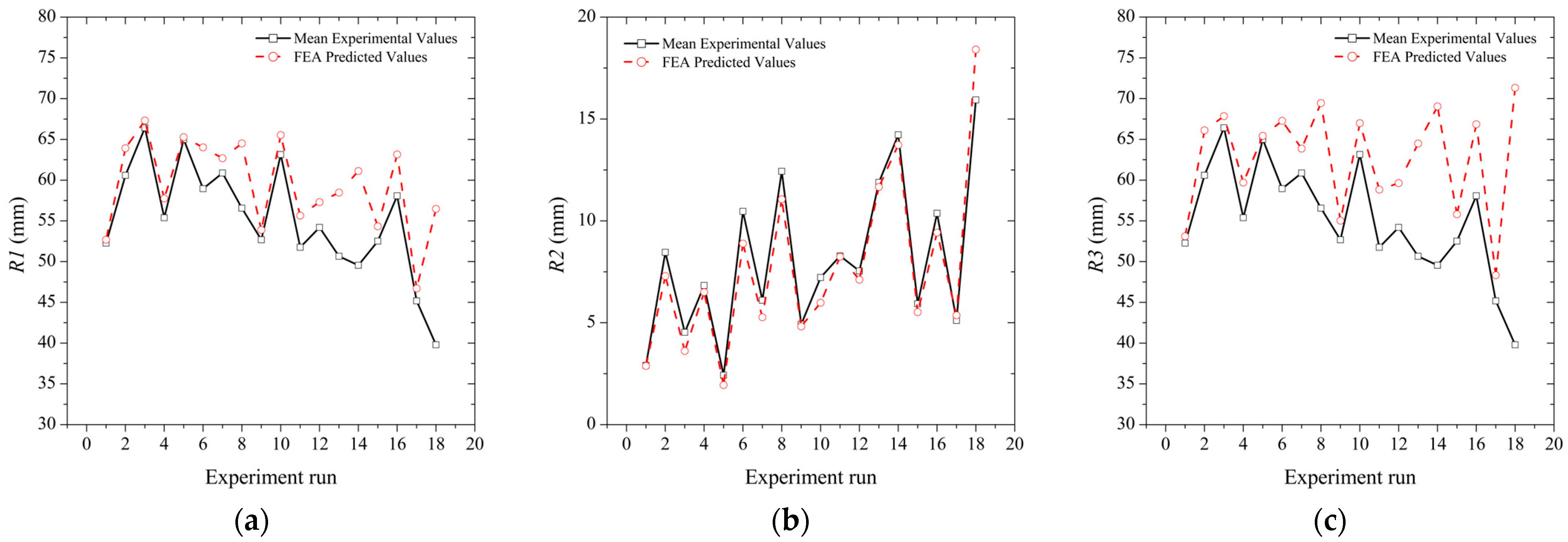
In this paper, the primary objective is to comprehensively investigate the shape-morphing behavior of PLA structures. We investigate the complex relationship between the morphing response, the printing parameters (printing speed, layer height, layer width, nozzle temperature, and bed temperature), and thermal stimulus through a systematic experimental characterization. By subjecting these structures to thermal stimulus, we explore their shape-morphing behavior, leveraging the unique properties of SMPs. The experimentation is further enriched by employing analysis of variance (ANOVA) to determine the significant impact of individual printing parameters and thermal stimulus on their change of shape. Consequently, regression analysis is conducted to develop empirical equations that predict the morphing behavior based on the chosen control factors. The observed morphing behavior is then simulated and validated using finite element analysis (FEA), which offers important insights into the structural performance under different thermal conditions.

2. Methodology

With the introduction of structures that can change shape in response to environmental changes, 4D printing opens a new chapter in the evolution of additive manufacturing. These novel structures, which are primarily made of Polylactic Acid (PLA), a well-known bio-sourced shape-memory polymer (SMP), have attracted a lot of attention due to their potential uses in a variety of industries, such as biomedical devices and adaptive architecture. To successfully comprehend and regulate their shape-morphing activity, research is still being carried out. The details of the printing process and the post-printing environments have a major impact on the final shape and functionality of these structures.

To thoroughly understand shape morphing in 4D-printed PLA structures, an extensive experimental methodology was developed. This approach aimed to reveal the complex interactions between various printing parameters and their impact on the morphing behaviors of the structures. The design and slicing of the sample set the stage for the next step, which is printing. After that, the sample is created utilizing fused deposition modeling (FDM) technology, which is an essential step in the creation of the physical product. The sample is allowed to cool at room temperature after printing. This stage is necessary for maintaining the structure’s stability, consistency of the material’s characteristics, and shape stability. The sample is ready for the activation phase after it has cooled, and this includes putting it in a controlled lab bath (thermostatic water bath, DK-420 model, Wincom Company, Ltd., Changsha, China). To simulate the external stimuli that cause the shape morphing, this stage is crucial. The employed bath can develop the targeted activation temperature, which then constitutes the stimulus for the specimen. Next, the sample’s activation and deformation are seen, demonstrating the material’s ability to adjust and change form in response to external stimuli. This change, which highlights the dynamic potential of 4D printing, is an essential aspect of the research. The deformed sample is then allowed to cool to ambient temperature. Measurements and data are carefully gathered during this phase, offering important insights into the morphing process and the elements controlling it.

2.1. Materials and Methods

The dimensions of the specimens utilized in the experiments are L = 70 mm, b = 3.5 mm, and h = 1.5 mm. The creation of the test specimens involved a detailed process starting from digital design to their physical formation. Initially, each specimen was designed using computer-aided design (CAD) software (Autodesk Inventor 2023). After designing, the specimens were prepared for 3D printing. This stage involved setting various printing parameters in the slicing software, which is crucial for achieving the desired print quality and functionality. Important parameters set at this stage included print speed, bed and nozzle temperatures, layer height, and layer width, each contributing significantly to the final physical attributes of the specimens.

The fabrication of test specimens was carried out using a K1 3D printer (Creality 3D Technology Co., Ltd., Shenzen, China). For this study, a high-quality PLA filament was selected, with a 1.75 mm diameter, presented in a clean white color (Devil Design, Mikołów). The specimens were subjected to a number of experimental processes in a lab water bath after printing. The PLA specimen is printed in its initial, undeformed state. This is the ‘zero strain energy’ state the reviewer refers to. It is important to clarify that at this stage, the beam is straight and has not undergone any deformation. This water bath can reach and sustain a particular temperature, which is known as the activation temperature. The specimens start to show signs of transformation at this temperature, reacting to the heat as an outside stimulus. A uniform exposure time of four minutes to the heat stimulus was maintained across all tests, ensuring consistency in the experimental conditions. This duration was experimentally observed to be sufficient for the sample to take its final/locked-in shape. The temperatures selected (thermal stimulus) are above the glass transition temperature of PLA. This is the ‘triggering’ process for the PLA beam. Once the PLA beam is removed from the bath and cooled down, it retains the bent shape, which is its ‘final’ or ‘locked-in’ shape. The recovery to the original straight shape is not part of this study.

2.2. Design of Experiments

The analysis was conducted using Minitab 17 statistical software, focusing on the effects of various printing factors. These factors included printing speed, layer height, layer width, nozzle temperature, bed temperature, and activation temperature. This study employed Taguchi’s L18 Design of Experiments (DoE) for its recognized accuracy and efficiency. A detailed outline of the control parameters and their levels is presented in the following

Table 1. Control parameters and their levels.

Code	Control Parameters	Unit	Level 1	Level 2	Level 3	Level 4	Level 5	Level 6
A	Activation Temperature	°C	76	80	84	88	92	96
B	Printing Speed	mm/s	50	80	110	-	-	-
C	Layer Height	mm	0.1	0.2	0.3	-	-	-
D	Layer Width	mm	0.36	0.4	0.48	-	-	-
E	Nozzle Temperature	°C	200	210	220	-	-	-
F	Bed Temperature	°C	30	45	60	-	-	-

.

The range of activation temperatures, from 76 °C to 96 °C, was chosen to thoroughly evaluate the material’s response to different thermal conditions. Printing speed, measured in mm/s, was varied across three levels to assess its impact on the final structure. Layer height, a critical factor in 3D printing, was tested at three different levels to balance between detail accuracy and printing speed. Finally, the layer width was also set at three distinct levels to understand its influence on the structural integrity and appearance of the printed object.

Table 2. The Taguchi L18 (6¹ × 3⁵) orthogonal array.

Experiment Run	Activation Temperature (°C)	Printing Speed (mm/s)	Layer Height (mm)	Layer Width (mm)	Nozzle Temperature (°C)	Bed Temperature (°C)
1	76	50	0.1	0.36	200	30
2	76	80	0.2	0.4	210	45
3	76	110	0.3	0.48	220	60
4	80	50	0.1	0.4	210	60
5	80	80	0.2	0.48	220	30
6	80	110	0.3	0.36	200	45
7	84	50	0.2	0.36	220	45
8	84	80	0.3	0.4	200	60
9	84	110	0.1	0.48	210	30
10	88	50	0.3	0.48	210	45
11	88	80	0.1	0.36	220	60
12	88	110	0.2	0.4	200	30
13	92	50	0.2	0.48	200	60
14	92	80	0.3	0.36	210	30
15	92	110	0.1	0.4	220	45
16	96	50	0.3	0.4	220	30
17	96	80	0.1	0.48	200	45
18	96	110	0.2	0.36	210	60

presents a comprehensive overview of the experimental runs, which were structured according to the Taguchi method. In this table, the columns represent the control factors, while the rows indicate the individual experimental runs. Each run is essentially a unique combination of factor levels. The cells within the table specify the level of each factor for a particular run.

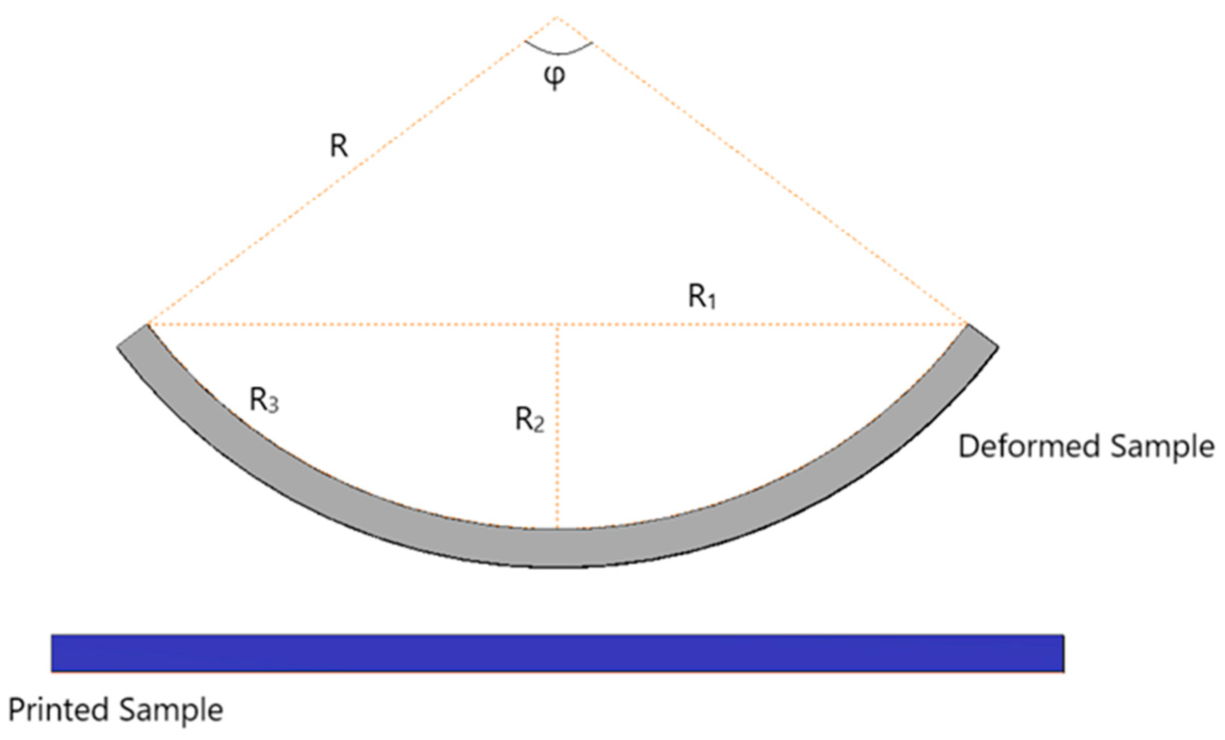
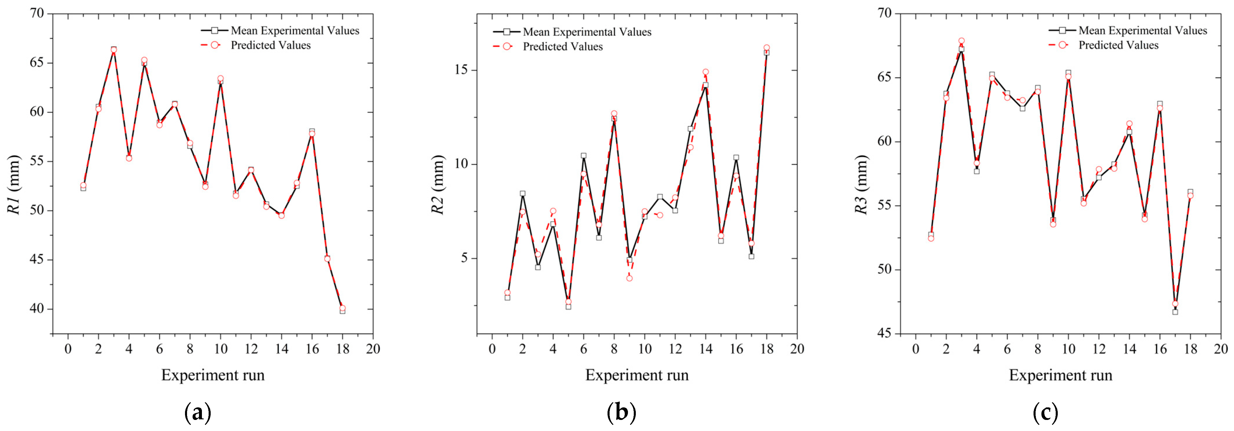
During the data acquisition stage, precise measurements of R1, R2, and R3 were obtained using Autodesk Inventor Professional software, which is known for its advanced measurement capabilities. The analysis focused on the deformed shape of the structure, with each parameter capturing a distinct aspect of the deformation:

• R1—Chord of Deformed Structure: This parameter represents the straight line distance between the two ends of the curve, essentially measuring the overall length of the deformed structure;
• R2—Beam Deflection: R2 measures the extent of deviation or displacement of the beam from its original position. It is a critical indicator of the degree of deformation experienced by the structure;
• R3—Internal Arc: This parameter captures the curvature within the deformed shape, providing insights into the internal bending and shape changes of the structure.

For a more comprehensive understanding, Figure 1 visually illustrates these parameters, offering a clearer perspective on their roles and relevance in analyzing the deformation of the structure. R is the radius of curvature of the arc, and ϕ is the angle subtended by the arc.

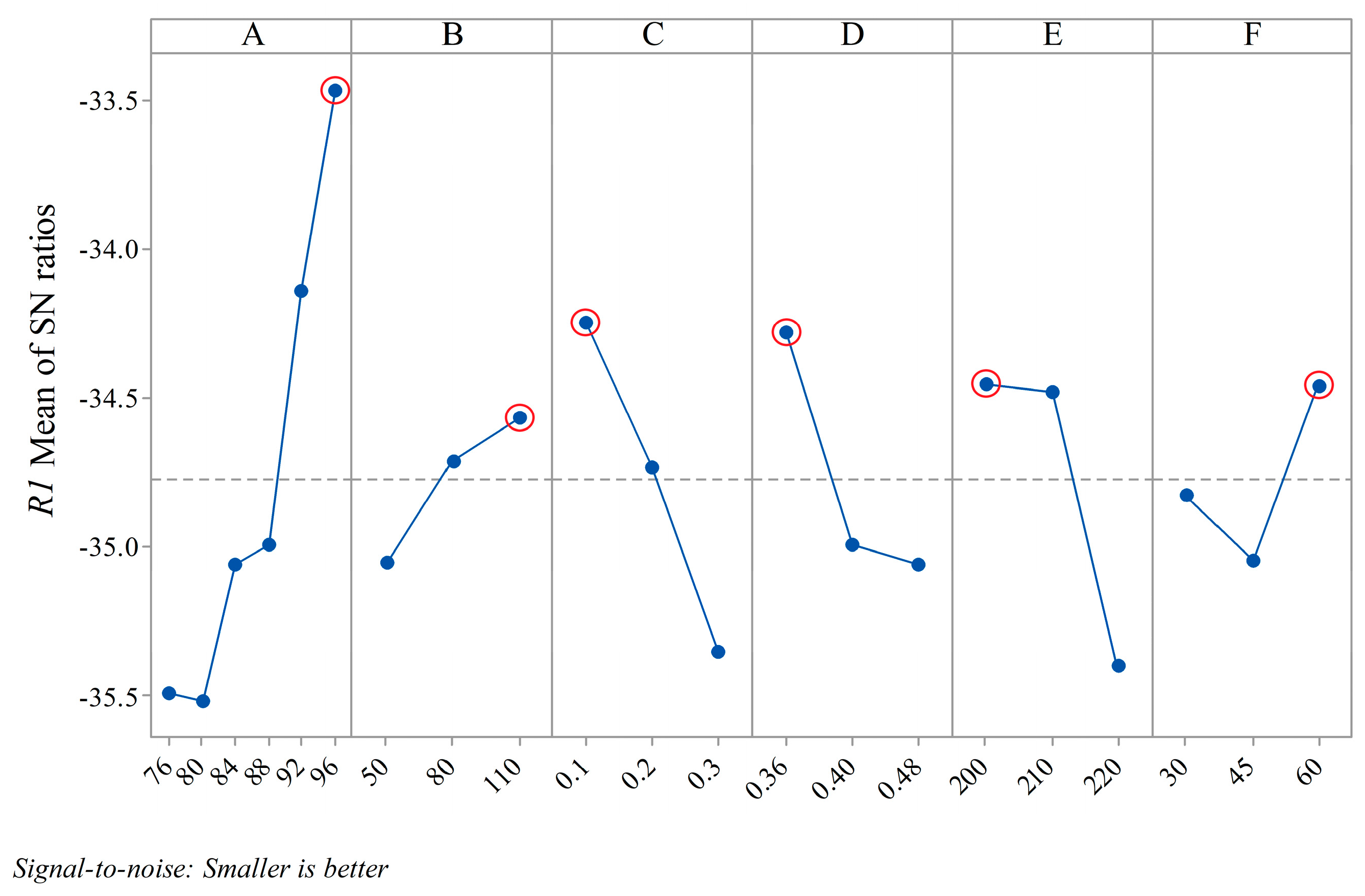
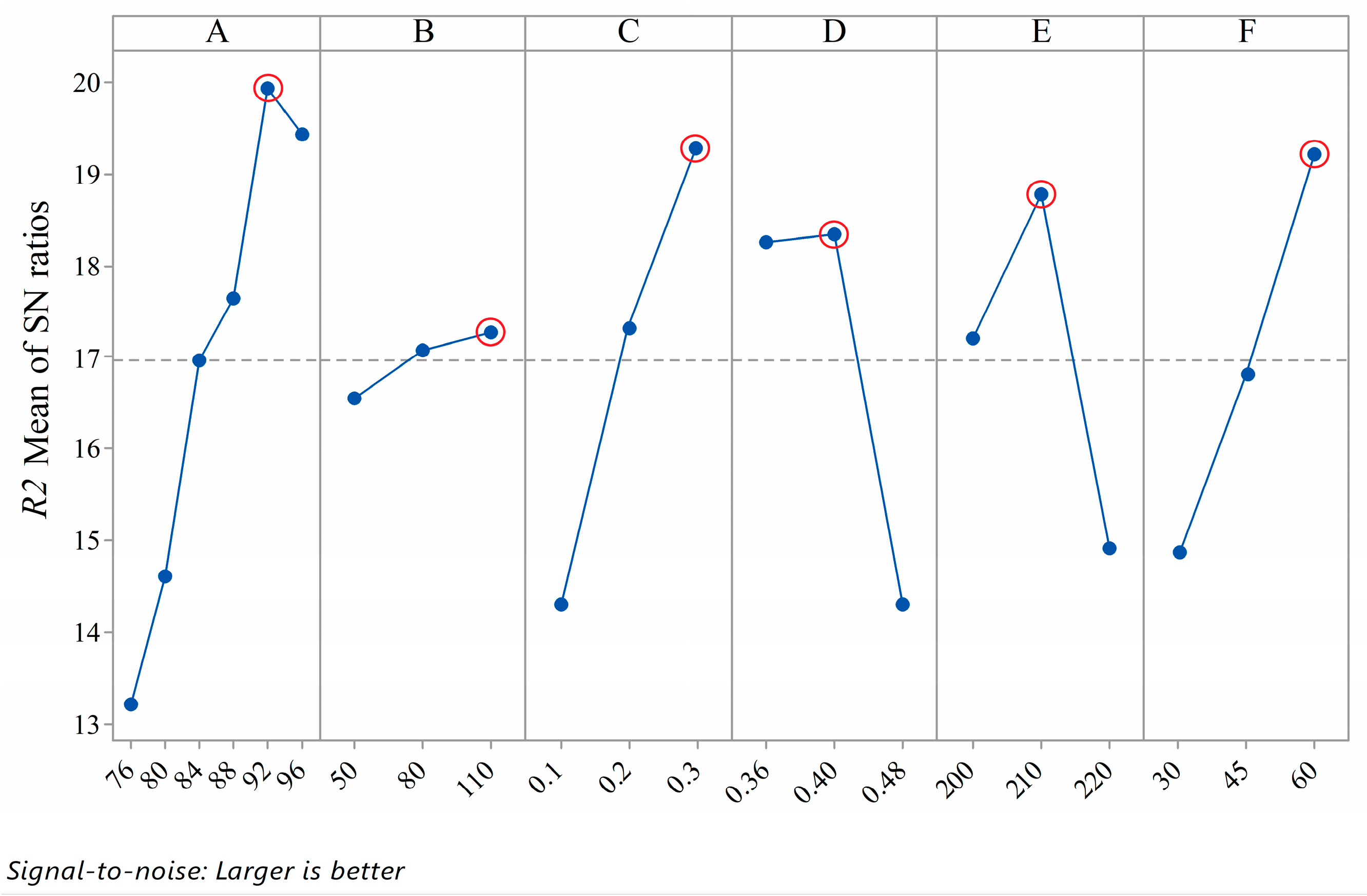
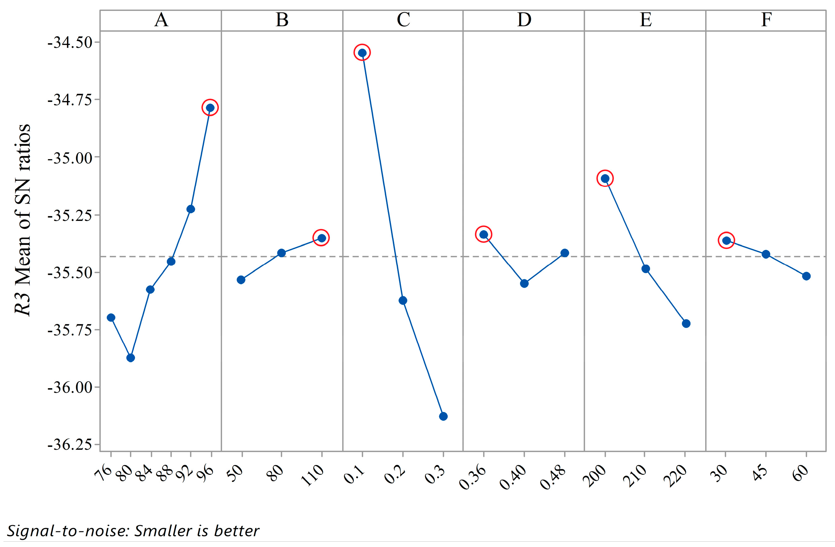
2.3. Main Effect Analysis

To assess the influence of each control factor on the response, the means and signal-to-noise (S/N) ratios are calculated. The S/N ratio, a measure of robustness, helps identify control factor configurations that effectively minimize variability or ‘noise’ in the process. In this study, the ‘Larger is better’ criterion was selected to maximize the response. This criterion is applicable to the R2 responses. Conversely, for the R1 and R3 responses, the ‘Smaller is better’ criterion was employed. The S/N ratios for these criteria are calculated using specific equations, designated as Equation (1) for the ‘Larger is bett’ and Equation (2) for the ‘Smaller is better’ [46]:

$$S/N=-10\cdot {\log }_{10}\left({\displaystyle \sum }_{i=1}^n\left(1/Y^2\right)/n\right),$$

(1)

$$S/N=-10\cdot {\log }_{10}\left({\displaystyle \sum }_{i=1}^n{Y}^2/n\right).$$

(2)

where Y denotes responses for the given factor level combination, and n is the number of responses in the factor level combination. These equations provide a quantitative basis for evaluating and optimizing the performance of the control factors in the experiment.

The response of each factor level in the context of a Taguchi experimental design can be effectively analyzed using the mean of the signal-to-noise (S/N) ratios and the mean response values. This approach is crucial for understanding how different levels of a factor influence the outcome of an experiment. For a given factor level, the mean of the S/N ratios is obtained by averaging the S/N ratios of all experiment runs where that particular level is present. Mathematically, it is represented as follows:

$$M_{\frac{S}{N}}=\frac{1}{k}{\displaystyle \sum }_{i=1}^k{(S/N)}_i.$$

(3)

Here, $k$ is the number of experimental runs that include the specific level of the factor being analyzed.

The mean response for each factor level involves averaging the response values for all the experimental runs where the factor level is present. The equation is given as:

$${\mathrm{M}}_{Response}=\frac{1}{k}{\displaystyle \sum }_{\mathrm{i}=1}^{\mathrm{k}}{\overline{R_x}}_i.$$

(4)

In this equation, ${\overline{R_x}}_i$ represents the average response value for the i-th experimental run.

2.4. Analysis of Variance (ANOVA)

The primary objective of ANOVA in this context is to assess the individual impact of each factor on the response variables R1, R2, and R3. The ANOVA process involves several key calculations [47]:

• Total Degrees of Freedom: This is calculated using $d{f}_{tot}=k-1$, where k represents the total number of experimental runs.
• Degrees of Freedom for Each Control Factor: Determined by $d{f}_i=l-1$, where i corresponds to each factor (A, B, C, D, E, F), and l is the total number of levels for each factor.
• Degrees of Freedom for Residual Error: Calculated using $d{f}_{error}=d{f}_{tot}-{\sum }_{i=1}^{n}d{f}_i$, where n is the number of control factors.

The total sum of squares ($S{S}_T$) represents the overall variation in the response values. It can be broken down into components attributable to the individual control factors and the residual error. This relationship is expressed in the following equation:

$$S{S}_T=S{S}_E+{\displaystyle \sum }_{i=1}^{n}S{S}_i,$$

(5)

where $S{S}_i$ is the sum of squares attributed to the i-th control factor, and $S{S}_E$ is the sum of squares due to residual error.

The total sum of squares, $S{S}_T$, quantifies the total variation in the response data and is calculated using the following equation:

$$S{S}_T={\displaystyle \sum }_{i=1}^m{\left(\overline{Y_i}-\overline{Y} \right)}^2,$$

(6)

where $\overline{Y_i}$ is the mean response value for the i-th experiment run, $\overline{Y}$ is the overall mean of the response values, and m is the number of experimental runs in the orthogonal array.

The mean sum of squares of the i-th factor represents the average of the squared deviations for a particular factor. It is a measure of the variance within the groups defined by that factor. The equation is $M{S}_i=\frac{S{S}_i}{d{f}_i}$. The equation for the F-ratio is $F_i=\frac{M{S}_i}{M{S}_E}$, where $M{S}_E$ is the mean sum of squares of the residual error [48]. A higher F-value indicates a more significant effect of the control factor on the response variable (R1, R2, or R3).

The percent contribution of a factor in an experiment, particularly in the context of ANOVA, is a measure of how much a specific factor contributes to the overall variability in the response variable. The formula to calculate the percent contribution of a factor is as follows:

$$contribution (\%)=\frac{S{S}_i}{S{S}_T}100 (\%).$$

(7)

A high percent contribution indicates that a small change in this factor will have a significant impact on the performance or outcome of the experiment.

3. Finite Element Modelling

In the finite element modeling conducted for this study, the heating process of the Polylactic Acid (PLA) structures was accurately represented using convective heat transfer principles. This process is described by the equation [49,50]:

$$\dot{Q}=hA\left(T_2-T_1\right),$$

(8)

where $\dot{Q}$ signifies the rate of heat transfer, h is the coefficient of heat transfer, A represents the surface area over which heat transfer occurs, $T_1$ is the initial temperature of the PLA structure, and $T_2$ is the activation temperature, equivalent to the temperature of the laboratory’s water bath. This equation is crucial in the simulation, as it determines the rate at which heat is transferred from the water bath to the PLA structure.

In the context of continuum mechanics, the deformation of a particle as it moves from its original position to a new position over time can be mathematically described using the concept of the deformation gradient. The initial position of a particle is denoted by X, and its position at a later time t is given by $x=x\left(X, t\right)$. The displacement vector $u=u\left(X, t\right)$ represents the change in position of the particle, pointing from its original location X to its new location x. The deformation gradient, F, is a fundamental tensor that captures all the information about the deformation and rotation of material elements in the body. It can be defined using the equation [49,50]:

$$F=\frac{\partial x}{\partial X}=I+\frac{\partial u}{\partial X}.$$

(9)

This equation represents the gradient of the current position with respect to the initial position, encapsulating how a differential element in the body moves and deforms. The term I is the identity tensor, which represents a state of no deformation. The second term is the gradient of the displacement vector, indicating how the displacement varies over the body.

In the finite element analysis of thermally induced deformation of PLA structures, understanding the interplay between mechanical and thermal properties is essential. The following equations form the basis of this analysis, explaining the complex relationships governing material behavior under thermal stimuli.

The equation of motion, represented as

$$\rho \frac{du}{d{t}^2}=\nabla \cdot \left(FS\right)+f_v,$$

(10)

is fundamental in describing the dynamic response of the PLA material. Here, ρ denotes the material’s density, S represents the second Piola–Kirchhoff stress tensor, and $f_v$ is the volumetric force. The stress–strain relationship is crucial in understanding how the material deforms under stress. This relationship is expressed as

$$S=C:{\epsilon }_{el},$$

(11)

where C is the elasticity tensor, and ${\epsilon }_{el}$ is the elastic strain tensor. This constitutive equation is key to modeling the elastic behavior of the PLA material under applied stresses.

Thermal strain is generally described by the equation

$${\epsilon }_{th}=a\left({\rm T}-{{\rm T}}_{ref}\right).$$

(12)

In this context, α represents the coefficient of thermal expansion (CTE), T is the current temperature, and ${{\rm T}}_{ref}$ is the reference temperature.

The CTE for different parts of the PLA structure is calculated using

$$a_n=\frac{\mathsf{\Delta }{L}_n}{L_0\mathsf{\Delta }T}.$$

(13)

Here, $a_n$ denotes the CTE for either the top or bottom part of the structure, $\mathsf{\Delta }{L}_n$ is the change in length of that part, $L_0$ is the initial length, and ΔT is the temperature change. Accurate calculation of the CTE is vital for precise thermal analysis in FEA.

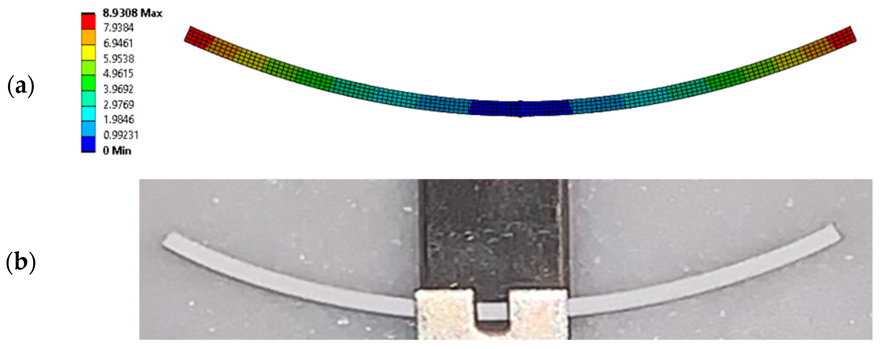
To accurately replicate the bending behavior characteristic of the shape-memory effect (SME) observed in shape-memory materials (SMMs), a strategy involving the concept of differential shrinking was employed. This approach is based on the principle of assigning different CTE to various parts of the structure, thereby inducing varying degrees of shrinkage in these parts, which in turn mimics the bending action seen in SME. The structure under study was modeled as consisting of two distinct parts. The post-deformation lengths of the top and bottom parts of the structure are determined using the following equations [50]:

$$\left\{\begin{array}{c}{L}_t=\left(R+0.25h_s\right)\phi \\ L_b=\left(R+0.75h_s\right)\phi \end{array}\right\}.$$

(14)

In these equations, $L_t$ and $L_b$ represent the lengths of the top and bottom parts, respectively, after deformation. $h_s$ is the height of the cross-section of the structure. These lengths are calculated at half the height of each of the top and the bottom parts of the structure, hence the use of 0.25$h_s$ and 0.75$h_s$.

The primary equation that governs the deformation of the PLA structure in response to thermal stimuli can be represented as follows:

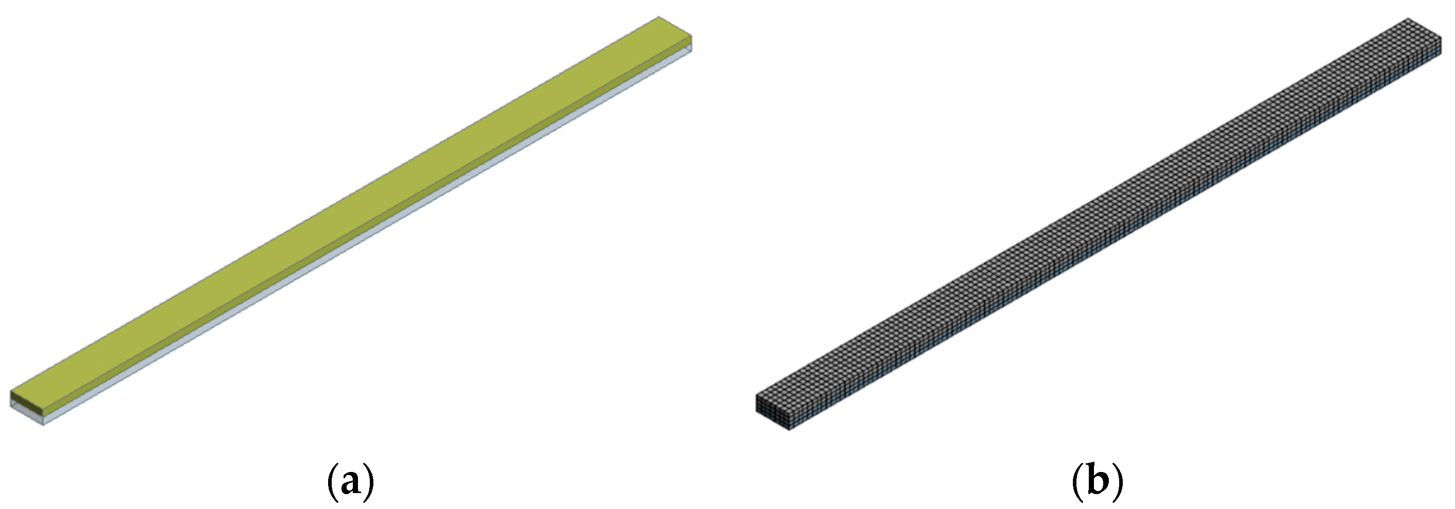
$$Ku=F+F_{\mathrm{th}}.$$

(15)

Here, $K$ is the global stiffness matrix of the structure, $u$ is the displacement vector, representing the deformation of the structure in response to the applied forces, $F$ is the vector of mechanical forces acting on the structure, including any external loads or constraints, and $F_{\mathrm{th}}$ is the thermal force vector, which arises due to the thermal expansion or contraction of the material as a result of temperature changes. The thermal force vector is calculated based on the material’s coefficient of thermal expansion (CTE), the temperature change, and the constraints of the structure and, thus, introduces the effects of temperature into the structural behavior. The FEA process involves discretizing the PLA structure into a finite number of elements, where each element’s behavior is described by the above equation. The global stiffness and the force vectors are assembled from the contributions of all these elements. The resulting system of equations is then solved numerically to find the displacement vector, which provides a detailed prediction of how each part of the PLA structure deforms in response to the combined effects of mechanical loads and thermal stimuli.

Our model, employing a CTE gradient/layering approach, is primarily designed to predict the maximum strain recovery for a given change in temperature based on the CTE and delta-Temp. It is important to note that in our current model, subsequent triggering of the PLA structures is not included. This means that while our model effectively handles a range of initial deformation levels (strains) up to the point of damage or fracture, it primarily focuses on the first activation cycle. The deformation in the previously triggered stage, which may vary widely, is considered as the starting point for each simulation. Our approach allows for the prediction of the final shape after the initial triggering but does not simulate repeated cycles of deformation and recovery. We acknowledge this as a limitation in the current scope of our model and suggest that future work could extend the model to include multiple triggering cycles. This would enhance the model’s applicability in scenarios where repeated shape-memory effects are critical.

4. Results and Discussion

4.1. Experimental Results and Analysis

4.1.1. S/N Analysis

In quality engineering, particularly when applying the Taguchi method, the S/N ratio is a vital metric. It measures how much the desired signal (or quality characteristic) stands out from the noise, which represents the variability or unwanted fluctuations in the process. A high S/N ratio indicates that the quality characteristic is significantly stronger and more consistent compared to the noise factors. In process optimization, the S/N ratio is key to determining performance. A higher S/N ratio suggests a more robust process where the impact of random variations is minimized. This is crucial in manufacturing and engineering, where achieving consistent and predictable outcomes is essential. The optimal level for any process parameter is identified by the highest S/N ratio. At this level, the process demonstrates maximum stability and minimal susceptibility to noise. In this study, these optimal levels are marked with circles in Figure 2, Figure 3 and Figure 4. This visual highlighting aids in quickly identifying which parameter levels yield the best performance in terms of quality characteristics. Focusing on these optimal levels allows for fine-tuning of the process parameters to achieve the best possible results.

One desirable characteristic is the minimization of the response R1. The optimal levels of the process parameters can be selected from Figure 2, indicated by the levels that produce the highest S/N ratio values, i.e., A6B3C1D1E1F3. Specifically, the optimal levels translate to specific settings for each process parameter level: activation temperature at level 6, which is 96 °C’ printing speed at level 3, equating to 110 mm/s; layer height at level 1, set at 0.1 mm; layer width at level 1, which is 0.36 mm; nozzle temperature at level 1, corresponding to 200 °C; and bed temperature at level 3, set at 60 °C.

For the response variable R2, the objective is to maximize its value. The optimal settings for the process parameters, identified from Figure 3 based on the highest S/N ratio values, are A5B3C3D2E2F3. These translate into specific process settings as follows: The activation temperature is optimally set at level 5, which is 92 °C, ideal for maximizing R2. The printing speed is maintained at level 3, equivalent to 110 mm/s, which is identified as the most effective speed for this response. The layer height is adjusted to level 3, or 0.3 mm, while the layer width is set at level 2, or 0.4 mm. The nozzle temperature is at level 2, set at 210 °C, and the bed temperature is kept at level 3, or 60 °C, effectively contributing to the maximization of the response R2. These settings collectively ensure that the process is finely tuned to achieve the highest possible response for R2.

In the case of the response variable R3, the target is to minimize its value. To determine the most effective settings for the process parameters, one can refer to Figure 4, where the optimal levels are indicated by the highest S/N ratio values. For R3, the optimal parameter levels (A6B3C1D1E1F1) have been identified as follows: The activation temperature is set at level 6, corresponding to 96 °C, which is the most effective level for minimizing R3. The printing speed is maintained at level 3, equating to 110 mm/s, which is identified as optimal for this specific response. The layer height is adjusted to level 1, set at 0.1 mm, while the layer width is set at level 1, or 0.36 mm. The nozzle temperature is at level 1, corresponding to 200 °C, optimal for the minimization objective. Lastly, the bed temperature is kept at level 1, or 30 °C.

4.1.2. ANOVA

ANOVA was employed to evaluate the influence of various control parameters on the response variables R1, R2, and R3, as indicated by their S/N ratios. The results of these analyses are presented in

Table 3. ANOVA results for R1 S/N ratios.

Code	DoF	Sum of Squares	Mean Squares	F	p	Contribution (%)
A	5	9.938	1.988	42.640	0.023	46.8
B	2	0.752	0.376	8.060	0.110	3.5
C	2	3.698	1.849	39.670	0.025	17.4
D	2	2.238	1.119	24.010	0.040	10.5
E	2	3.462	1.731	37.130	0.026	16.3
F	2	1.050	0.525	11.270	0.082	4.9
Residual error	2	0.093	0.047	-	-	0.4
Total	17	21.231	-	-	-	100.0

,

Table 4. ANOVA results for R2 S/N ratios.

Code	DoF	Sum of Squares	Mean Squares	F	p	Contribution (%)
A	5	104.909	20.982	1.350	0.476	27.7
B	2	1.677	0.839	0.050	0.949	0.4
C	2	75.979	37.990	2.450	0.290	20.1
D	2	63.356	31.678	2.040	0.329	16.7
E	2	44.837	22.419	1.450	0.409	11.8
F	2	56.876	28.438	1.840	0.353	15.0
Residual error	2	30.995	15.497	-	-	8.2
Total	17	378.628	-	-	-	100.0

, and

Table 5. ANOVA results for R3 S/N ratios.

Code	DoF	Sum of Squares	Mean Squares	F	p	Contribution (%)
A	5	2.240	0.448	7.600	0.120	19.0
B	2	0.104	0.052	0.880	0.532	0.9
C	2	7.855	3.927	66.650	0.015	66.8
D	2	0.138	0.069	1.170	0.461	1.2
E	2	1.234	0.617	10.470	0.087	10.5
F	2	0.074	0.037	0.620	0.616	0.6
Residual error	2	0.118	0.059			1.0
Total	17	11.762				100

, respectively. The ANOVA was conducted with a 95% confidence level (significance level of 5%).

For R1 (Table 3), the ANOVA results show that the activation temperature was the most significant factor, contributing 46.8% to the S/N ratio with an F-value of 42.640 and a p-value of 0.023. Other factors like layer height and nozzle temperature also showed notable contributions of 17.4% and 16.3%, respectively. Layer width had lesser but still significant impact on R1.

In the case of R2 (Table 4), the activation temperature again showed the highest contribution at 27.7%, although with a lower F-value of 1.350 and a higher p-value of 0.476, indicating a less significant impact compared to R1. Layer height, layer width and bed temperature contributed 20.1%, 16.7% and 15.0%, respectively, while the other factors had minimal impact. The residual error accounted for 8.2% of the total variance.

For R3 (Table 5), layer height emerged as the most influential factor, contributing a substantial 66.8% to the S/N ratio with a high F-value of 66.650 and a low p-value of 0.015. Nozzle temperature also had a notable impact, with a 10.5% contribution. Other factors like activation temperature, printing speed, layer width, and bed temperature showed relatively minor contributions.

From these ANOVA results, it is evident that certain factors have more significant impacts on the 4D shape-morphing properties of the structures. For instance, layer height predominantly influences R3, while activation temperature has a more pronounced effect on R1 and R2. These insights are crucial for optimizing the 3D printing process parameters to achieve the desired smart performance in the final printed structures.

4.1.3. Regression Analysis

In this research, regression analysis was employed to establish the relationships between independent variables (control parameters) and dependent variables (responses R1, R2, and R3). The effectiveness of these relationships is quantified using the R-squared (R²) value, a statistical measure that assesses the validity of the regression model. R² indicates how well the independent variables explain the variability in the dependent variables.

The predictive equation for the mean R1 (in mm) response, derived from regression analysis, is expressed as

$$R1=28.1-0.624A-0.044B+35.76C+37.3D+0.3070E-0.0622F,$$

(16)

with an R² value of 86.35%. This high R² value suggests a strong correlation between the model and the observed data, indicating the model’s reliability in predicting the R1 response based on the control parameters.

Similarly, the predictive equation for the mean R2 (in mm) response is formulated as

$$R2=10.1+0.2718A+0.0111B+21.05C-30.58D-0.1059E+0.0972F,$$

(17)

with an R² value of 80.51%. Although slightly lower than that for R1, this value still reflects a good level of predictability of the R2 response from the control parameters.

For the mean R3 response, the regression analysis yields the equation.

$$R3=30.2-0.3163A-0.0199B+52.96C+5.21D+0.2081E+0.0343F,$$

(18)

with an R² value of 93.40%. This high R² value indicates an excellent fit between the model and the observed data, suggesting that the model is highly effective in predicting the R3 response.

In the field of multiple regression analysis, the R² value is a critical indicator of the model’s predictive power. Ideally, R² should range between 0.8 and 1.0 for the model to be considered highly effective. In the context of this study, the mathematical equations developed through regression analysis have R² values within this ideal range. Consequently, these equations are well-suited for predicting the shape-morphing behavior of 4D printing PLA structures.

To assess the accuracy and reliability of the developed regression models, a crucial step involved comparing the predicted values from the models with actual experimental results. This comparison is essential for validating the effectiveness of the regression models in accurately predicting outcomes. The comparison was visualized through plots that are illustrated in Figure 5. Generally, the plots showed a high degree of similarity between the experimental and predicted values, indicating that the regression models were successful in closely approximating the actual behavior of the 4D printing PLA structures. This level of accuracy is crucial for practical applications, as it provides confidence in using these models for design and optimization purposes in the field of 4D printing technology.

4.2. FEA Results

The structure under study was modeled as consisting of two distinct parts, as depicted in Figure 6a. Each part was assigned a different CTE value. The rationale behind this approach is that when these parts are subjected to thermal changes, they shrink at different rates due to their distinct CTE values. This differential shrinking across the parts results in the bending effect, which is a crucial aspect of the SME in SMMs.

To determine the appropriate CTE values for the top and bottom parts of the structure, an analysis of their arc length differences was conducted. By calculating the difference in arc lengths, the required CTE values for each part were estimated. These calculated CTE values were then incorporated into the FEA models. The corresponding results are shown in

Table 6. CTE values of top and bottom parts of the sample for each experiment run.

Experiment Run	at (°C−1)	ab (°C−1)
1	−4.98 × 10−3	−4.88 × 10−3
2	−1.70 × 10−3	−1.46 × 10−3
3	−7.45 × 10−4	−6.26 × 10−4
4	−3.22 × 10−3	−3.02 × 10−3
5	−1.25 × 10−3	−1.19 × 10−3
6	−1.53 × 10−3	−1.26 × 10−3
7	−1.78 × 10−3	−1.63 × 10−3
8	−1.29 × 10−3	−9.78 × 10−4
9	−3.97 × 10−3	−3.83 × 10−3
10	−9.98 × 10−4	−8.40 × 10−4
11	−3.28 × 10−3	−3.06 × 10−3
12	−2.90 × 10−3	−2.71 × 10−3
13	−2.44 × 10−3	−2.15 × 10−3
14	−1.85 × 10−3	−1.51 × 10−3
15	−3.38 × 10−3	−3.24 × 10−3
16	−1.35 × 10−3	−1.13 × 10−3
17	−4.75 × 10−3	−4.62 × 10−3
18	−2.67 × 10−3	−2.24 × 10−3

.

The CTE values of Table 6 can be implemented into the FEA model. To determine the most suitable element size for mesh generation in the FEA model, a mesh sensitivity analysis is performed. This analysis is crucial to ensure that the mesh is fine enough to capture the necessary details of the model while also being coarse enough to keep computational costs reasonable. When the element size is reduced to less than 1 mm, the values for R1, R2, and R3 start to converge towards a consistent value. An element size of 0.5 mm is selected (Figure 6b). This size not only falls within the range where the response variables converge but also offers a fine enough mesh to ensure detailed and accurate modeling.

In this study, Figure 7 compares the outcomes of FEA simulations with actual experimental observations of a printed structure. This comparison is diagnostic for validating the accuracy and applicability of the FEA model developed. For both the simulation and the experimental test, the structure was produced under specific conditions (experimental run 4): a printing speed of 50 mm/s, layer height of 0.1 mm, layer width of 0.4 mm, nozzle temperature set at 210 °C, bed temperature at 60 °C, and an activation temperature of 80 °C. Figure 7a displays the results from the FEA simulation. The simulation provides a theoretical insight into how the structure is expected to deform in response to the set conditions. Conversely, Figure 7b illustrates the actual deformation observed in the structure following its immersion in a laboratory bath.

In assessing the accuracy of the FEA model for predicting responses R1, R2, and R3, a comparison was made between the mean values obtained from experimental runs and those derived from the simulation. This comparison is crucial for evaluating the model’s precision and identifying areas for improvement. For the R1 response, a significant proportion of the experiment runs showed close agreement between the experimental and simulated values. Figure 8a illustrates this comparison, showcasing the mean R1 values from both the experiments and the FEA model. The similarity in these values indicates a strong correlation and reliability of the FEA model for the R1 response. In the case of the R2 response, as depicted in Figure 8b, the FEA model also demonstrated a good level of agreement with the experimental data, although with some variations. These variations might be attributed to factors such as slight discrepancies in material properties, boundary conditions, or assumptions made in the simulation process. Similarly, for the R3 response, Figure 8c compares the mean values from experiments with those predicted by the FEA model. While there is a good level of agreement, some variations are observed, which could be due to factors like the precision of the experimental measurements, the complexity of the model, or the sensitivity of the response to specific parameters.

The material chosen, while exhibiting thermoplastic behavior typical of many polymers when heated above its glass transition temperature, was selected for its improved performance in maintaining a deformed shape upon cooling. This property is particularly valuable in aerospace applications where components often require permanent, intricate adjustments to optimize performance under varying operational conditions. The focus on the deformation and stabilization phases, rather than the recovery characteristic typical of SMPs, aligns with the practical requirements of applications, where the permanence of the deformed shape can be more relevant than the material’s ability to return to its original form. This approach provides insights into the material’s suitability for specific applications, such as the fabrication of morphing structures, where the emphasis is on reliable, long-term performance in demanding environmental conditions.

5. Conclusions

In conclusion, this study marks a significant advancement in the field of 4D printing, particularly in understanding the shape-morphing behavior of PLA structures. The research highlights the critical role of specific printing parameters in influencing this behavior, offering valuable insights for both theoretical understanding and practical applications. Key findings include the following:

• Activation temperature and layer height emerged as significant factors influencing the shape-morphing behavior, as revealed by the S/N ratio analysis and ANOVA results;
• The precision in setting the printing speed, layer width, nozzle temperature, and bed temperature was found to be crucial in achieving the desired shape-morphing characteristics;
• Regression models developed for predicting the responses R1, R2, and R3 demonstrated strong correlations with observed data, highlighting the interplay between these printing parameters and the shape-morphing outcomes;
• The FEA modeling successfully predicted the performance of the structures, demonstrating its potential as an effective design tool in 4D printing;
• The ability of FEA modeling to closely predict the experimental outcomes suggests its utility in the design phase, allowing for the optimization of printing parameters before actual production.

These insights not only enhance our understanding of the complex dynamics in 4D printing but also provide a foundation for optimizing the printing process to harness the full potential of shape-morphing materials in various applications. This study paves the way for future research and development in the field, focusing on the intricate relationship between printing parameters and the functional capabilities of 4D-printed structures.

References

1. Momeni, F.; Liu, X.; Ni, J. A Review of 4D Printing. Mater. Des. 2017, 122, 42–79. [Google Scholar] [CrossRef]
2. Chu, H.; Yang, W.; Sun, L.; Cai, S.; Yang, R.; Liang, W.; Yu, H.; Liu, L. 4D Printing: A Review on Recent Progresses. Micromachines 2020, 11, 796. [Google Scholar] [CrossRef] [PubMed]
3. Kuang, X.; Roach, D.J.; Wu, J.; Hamel, C.M.; Ding, Z.; Wang, T.; Dunn, M.L.; Qi, H.J. Advances in 4D Printing: Materials and Applications. Adv. Funct. Mater. 2019, 29, 1805290. [Google Scholar] [CrossRef]
4. Khalid, M.Y.; Arif, Z.U.; Noroozi, R.; Zolfagharian, A.; Bodaghi, M. 4D Printing of Shape Memory Polymer Composites: A Review on Fabrication Techniques, Applications, and Future Perspectives. J. Manuf. Process. 2022, 81, 759–797. [Google Scholar] [CrossRef]
5. Yarali, E.; Baniasadi, M.; Zolfagharian, A.; Chavoshi, M.; Arefi, F.; Hossain, M.; Bastola, A.; Ansari, M.; Foyouzat, A.; Dabbagh, A.; et al. Magneto-/Electro-responsive Polymers toward Manufacturing, Characterization, and Biomedical/Soft Robotic Applications. Appl. Mater. Today 2022, 26, 101306. [Google Scholar] [CrossRef]
6. Zafar, M.Q.; Zhao, H. 4D Printing: Future Insight in Additive Manufacturing. Met. Mater. Int. 2019, 26, 564–585. [Google Scholar] [CrossRef]
7. Hua, M.; Wu, D.; Wu, S.; Ma, Y.; Alsaid, Y.; He, X. 4D Printable Tough and Thermoresponsive Hydrogels. ACS Appl. Mater. Interfaces 2021, 13, 12689–12697. [Google Scholar] [CrossRef]
8. Zhang, Y.; Wang, Q.; Yi, S.; Lin, Z.; Wang, C.; Chen, Z.; Jiang, L. 4D Printing of Magnetoactive Soft Materials for On-Demand Magnetic Actuation Transformation. ACS Appl. Mater. Interfaces 2021, 13, 4174–4184. [Google Scholar] [CrossRef]
9. Rastogi, P.; Kandasubramanian, B. Breakthrough in the Printing Tactics for Stimuli-Responsive Materials: 4D Printing. Chem. Eng. J. 2019, 366, 264–304. [Google Scholar] [CrossRef]
10. Sonatkar, J.; Kandasubramanian, B.; Ismail, S.O. 4D Printing: Pragmatic Progression in Biofabrication. Eur. Polym. J. 2022, 169, 111128. [Google Scholar] [CrossRef]
11. Akbar, I.; El Hadrouz, M.; El Mansori, M.; Lagoudas, D. Toward Enabling Manufacturing Paradigm of 4D Printing of Shape Memory Materials: Open Literature Review. Eur. Polym. J. 2022, 168, 111106. [Google Scholar] [CrossRef]
12. Zhang, Z.; Demir, K.G.; Gu, G.X. Developments in 4D-Printing: A Review on Current Smart Materials, Technologies, and Applications. Int. J. Smart Nano Mater. 2019, 10, 205–224. [Google Scholar] [CrossRef]
13. Kačergis, L.; Mitkus, R.; Sinapius, M. Influence of Fused Deposition Modeling Process Parameters on the Transformation of 4D Printed Morphing Structures. Smart Mater. Struct. 2019, 28, 105042. [Google Scholar] [CrossRef]
14. Noroozi, R.; Bodaghi, M.; Jafari, H.; Zolfagharian, A.; Fotouhi, M. Shape-Adaptive Metastructures with Variable Bandgap Regions by 4D Printing. Polymers 2020, 12, 519. [Google Scholar] [CrossRef] [PubMed]
15. Mahmood, A.; Akram, T.; Shenggui, C.; Chen, H. Revolutionizing Manufacturing: A Review of 4D Printing Materials, Stimuli, and Cutting-Edge Applications. Compos. B Eng. 2023, 266, 110952. [Google Scholar] [CrossRef]
16. Khalid, M.Y.; Arif, Z.U.; Ahmed, W. 4D Printing: Technological and Manufacturing Renaissance. Macromol. Mater. Eng. 2022, 307, 2200003. [Google Scholar] [CrossRef]
17. Jones, M.P.; Murali, G.G.; Laurin, F.; Robinson, P.; Bismarck, A. Functional Flexibility: The Potential of Morphing Composites. Compos. Sci. Technol. 2022, 230, 109792. [Google Scholar] [CrossRef]
18. Sun, J.; Guan, Q.; Liu, Y.; Leng, J. Morphing Aircraft Based on Smart Materials and Structures: A State-of-the-Art Review. J. Intell. Mater. Syst. Struct. 2016, 27, 2289–2312. [Google Scholar] [CrossRef]
19. Ashir, M.; Hindahl, J.; Nocke, A.; Cherif, C. Development of an Adaptive Morphing Wing Based on Fiber-Reinforced Plastics and Shape Memory Alloys. J. Ind. Text. 2020, 50, 114–129. [Google Scholar] [CrossRef]
20. Ameta, K.L.; Solanki, V.S.; Singh, V.; Devi, A.P.; Chundawat, R.S.; Haque, S. Critical Appraisal and Systematic Review of 3D & 4D Printing in Sustainable and Environment-Friendly Smart Manufacturing Technologies. Sustain. Mater. Technol. 2022, 34, e00481. [Google Scholar] [CrossRef]
21. Ntouanoglou, K.; Stavropoulos, P.; Mourtzis, D. 4D Printing Prospects for the Aerospace Industry: A Critical Review. Procedia Manuf. 2018, 18, 120–129. [Google Scholar] [CrossRef]
22. Zhao, W.; Yue, C.; Liu, L.; Leng, J.; Liu, Y. Mechanical Behavior Analyses of 4D Printed Metamaterials Structures with Excellent Energy Absorption Ability. Compos. Struct. 2023, 304, 116360. [Google Scholar] [CrossRef]
23. Ma, B.; Zhang, Y.; Li, J.; Chen, D.; Liang, R.; Fu, S.; Li, D. 4D Printing of Multi-Stimuli Responsive Rigid Smart Composite Materials with Self-Healing Ability. Chem. Eng. J. 2023, 466, 143420. [Google Scholar] [CrossRef]
24. Brischetto, S.; Torre, R.; Ferro, C.G. Experimental Evaluation of Mechanical Properties and Machine Process in Fused Deposition Modelling Printed Polymeric Elements. Adv. Intell. Syst. Comput. 2020, 975, 377–389. [Google Scholar] [CrossRef]
25. Zaman, U.K.U.; Boesch, E.; Siadat, A.; Rivette, M.; Baqai, A.A. Impact of Fused Deposition Modeling (FDM) Process Parameters on Strength of Built Parts Using Taguchi’s Design of Experiments. Int. J. Adv. Manuf. Technol. 2019, 101, 1215–1226. [Google Scholar] [CrossRef]
26. Patil, P.; Singh, D.; Raykar, S.J.; Bhamu, J. Multi-Objective Optimization of Process Parameters of Fused Deposition Modeling (FDM) for Printing Polylactic Acid (PLA) Polymer Components. Mater. Today Proc. 2021, 45, 4880–4885. [Google Scholar] [CrossRef]
27. Weber, R.; Kuhlow, M.; Spierings, A.B.; Wegener, K. 4D Printed Assembly of Sensors and Actuators in Complex Formed Metallic Lightweight Structures. J. Manuf. Process 2023, 90, 406–417. [Google Scholar] [CrossRef]
28. Fallah, A.; Asif, S.; Gokcer, G.; Koc, B. 4D Printing of Continuous Fiber-Reinforced Electroactive Smart Composites by Coaxial Additive Manufacturing. Compos. Struct. 2023, 316, 117034. [Google Scholar] [CrossRef]
29. Mahmood, A.; Akram, T.; Chen, H.; Chen, S. On the Evolution of Additive Manufacturing (3D/4D Printing) Technologies: Materials, Applications, and Challenges. Polymers 2022, 14, 4698. [Google Scholar] [CrossRef]
30. Joshi, S.C.; Sheikh, A.A. 3D Printing in Aerospace and Its Long-Term Sustainability. Virtual Phys. Prototyp. 2015, 10, 175–185. [Google Scholar] [CrossRef]
31. Jian, B.; Demoly, F.; Zhang, Y.; Qi, H.J.; André, J.C.; Gomes, S. Origami-Based Design for 4D Printing of 3D Support-Free Hollow Structures. Engineering 2022, 12, 70–82. [Google Scholar] [CrossRef]
32. Tao, R.; Ji, L.; Li, Y.; Wan, Z.; Hu, W.; Wu, W.; Liao, B.; Ma, L.; Fang, D. 4D Printed Origami Metamaterials with Tunable Compression Twist Behavior and Stress-Strain Curves. Compos. B Eng. 2020, 201, 108344. [Google Scholar] [CrossRef]
33. Liu, G.; Zhao, Y.; Wu, G.; Lu, J. Origami and 4D Printing of Elastomer-Derived Ceramic Structures. Sci. Adv. 2018, 4, 641–658. [Google Scholar] [CrossRef]
34. Zhou, T.; Zhou, Y.; Hua, Z.; Yang, Y.; Zhou, C.; Ren, L.; Zhang, Z.; Zang, J. 4D Printing High Temperature Shape-Memory Poly(Ether–Ether–Ketone). Smart Mater. Struct. 2021, 30, 115006. [Google Scholar] [CrossRef]
35. Zhang, J.; Yin, Z.; Ren, L.; Liu, Q.; Ren, L.; Yang, X.; Zhou, X. Advances in 4D Printed Shape Memory Polymers: From 3D Printing, Smart Excitation, and Response to Applications. Adv. Mater. Technol. 2022, 7, 2101568. [Google Scholar] [CrossRef]
36. Zhang, B.; Li, H.; Cheng, J.; Ye, H.; Hosein Sakhaei, A.; Yuan, C.; Rao, P.; Zhang, Y.-F.; Chen, Z.; Wang, R.; et al. Mechanically Robust and UV-Curable Shape-Memory Polymers for Digital Light Processing Based 4D Printing. Adv. Mater. 2021, 33, 2101298. [Google Scholar] [CrossRef]
37. Testoni, O.; Lumpe, T.; Huang, J.L.; Wagner, M.; Bodkhe, S.; Zhakypov, Z.; Spolenak, R.; Paik, J.; Ermanni, P.; Muñoz, L.; et al. A 4D Printed Active Compliant Hinge for Potential Space Applications Using Shape Memory Alloys and Polymers. Smart Mater. Struct. 2021, 30, 085004. [Google Scholar] [CrossRef]
38. Costanza, G.; Tata, M.E. Shape Memory Alloys for Aerospace, Recent Developments, and New Applications: A Short Review. Materials 2020, 13, 1856. [Google Scholar] [CrossRef] [PubMed]
39. Chen, S.; Li, J.; Shi, H.; Chen, X.; Liu, G.; Meng, S.; Lu, J. Lightweight and Geometrically Complex Ceramics Derived from 4D Printed Shape Memory Precursor with Reconfigurability and Programmability for Sensing and Actuation Applications. Chem. Eng. J. 2023, 455, 140655. [Google Scholar] [CrossRef]
40. Liu, G.; Zhang, X.; Lu, X.; Zhao, Y.; Zhou, Z.; Xu, J.; Yin, J.; Tang, T.; Wang, P.; Yi, S.; et al. 4D Additive–Subtractive Manufacturing of Shape Memory Ceramics. Adv. Mater. 2023, 35, 2302108. [Google Scholar] [CrossRef] [PubMed]
41. Patadiya, J.; Gawande, A.; Joshi, G.; Kandasubramanian, B. Additive Manufacturing of Shape Memory Polymer Composites for Futuristic Technology. Ind. Eng. Chem. Res. 2021, 60, 15885–15912. [Google Scholar] [CrossRef]
42. Pyo, Y.; Kang, M.; Jang, J.Y.; Park, Y.; Son, Y.H.; Choi, M.C.; Ha, J.W.; Chang, Y.W.; Lee, C.S. Design of a Shape Memory Composite(SMC) Using 4D Printing Technology. Sens. Actuators A Phys. 2018, 283, 187–195. [Google Scholar] [CrossRef]
43. Pivar, M.; Gregor-Svetec, D.; Muck, D. Effect of Printing Process Parameters on the Shape Transformation Capability of 3D Printed Structures. Polymers 2022, 14, 117. [Google Scholar] [CrossRef] [PubMed]
44. Solomon, I.J.; Sevvel, P.; Gunasekaran, J. A Review on the Various Processing Parameters in FDM. Mater. Today Proc. 2021, 37, 509–514. [Google Scholar] [CrossRef]
45. Nam, S.; Pei, E. The Influence of Shape Changing Behaviors from 4D Printing through Material Extrusion Print Patterns and Infill Densities. Materials 2020, 13, 3754. [Google Scholar] [CrossRef] [PubMed]
46. Methods and Formulas for Analyze Taguchi Design—Minitab. Available online: https://support.minitab.com/en-us/minitab/21/help-and-how-to/statistical-modeling/doe/how-to/taguchi/analyze-taguchi-design/methods-and-formulas/methods-and-formulas/ (accessed on 16 June 2023).
47. Montgomery, D.C. Design and Analysis of Experiments; Wiley: Hoboken, NJ, USA, 2019; 688p, ISBN 978-1-119-49244-3. [Google Scholar]
48. Bademlioglu, A.H.; Canbolat, A.S.; Yamankaradeniz, N.; Kaynakli, O. Investigation of Parameters Affecting Organic Rankine Cycle Efficiency by Using Taguchi and ANOVA Methods. Appl. Therm. Eng. 2018, 145, 221–228. [Google Scholar] [CrossRef]
49. Cheah, D.S.; Alshebly, Y.S.; Mohamed Ali, M.S.; Nafea, M. Development of 4D-Printed Shape Memory Polymer Large-Stroke XY Micropositioning Stages. J. Micromech. Microeng. 2022, 32, 065006. [Google Scholar] [CrossRef]
50. Alshebly, Y.S.; Nafea, M. Effects of Printing Parameters on 4D-Printed PLA Actuators. Smart Mater. Struct. 2023, 32, 064008. [Google Scholar] [CrossRef]
Figure 1. Schematic description of the deformed shape parameters. R1 is the chord connecting the two ends of the curve, R2 indicates the deflection, and R3 is the internal arc.
Aerospace 11 00134 g001
Figure 2. R1 mean of S/N ratios for each factor.
Aerospace 11 00134 g002
Figure 3. R2 mean of S/N ratios for each factor.
Aerospace 11 00134 g003
Figure 4. R3 mean of S/N ratios for each factor.
Aerospace 11 00134 g004
Figure 5. Comparison of experimental and predicted values of (a) R1, (b) R2, and (c) R3.
Aerospace 11 00134 g005
Figure 6. Model of the sample (a) geometry and (b) mesh with 0.5 mm element size.
Aerospace 11 00134 g006
Figure 7. Shape morphing of a PLA beam at 80 °C. (a) finite element prediction and (b) experimental result.
Aerospace 11 00134 g007
Figure 8. Comparison of experimental and FEA values of (a) R1, (b) R2, and (c) R3.
Aerospace 11 00134 g008