Article

Research on Unmanned Aerial Vehicle Cluster Collaborative Countermeasures Based on Dynamic Non-Zero-Sum Game under Asymmetric and Uncertain Information

1
College of Automation, Northwestern Polytechnical University, Xi’an 710000, China
2
College of Mathematics and Statistics, Northwestern Polytechnical University, Xi’an 710000, China
3
College of Cyberspace Security, Northwestern Polytechnical University, Xi’an 710000, China
4
Engineering Training Centre, Northwestern Polytechnical University, Xi’an 710000, China
*
Authors to whom correspondence should be addressed.
Aerospace 2023, 10(8), 711; https://doi.org/10.3390/aerospace10080711
Submission received: 27 June 2023 / Revised: 31 July 2023 / Accepted: 31 July 2023 / Published: 15 August 2023

Abstract

:
Unmanned aerial vehicle (UAV) swarm coordinated confrontation is a hot topic in academic research at home and abroad, and dynamic maneuver decision-making is one of the most important research fields for UAV countermeasures. Aiming at the complexity, uncertainty and confrontation of UAV cooperative confrontation, concepts such as relative advantage degree and advantage coefficient are introduced, and game theory is used as a framework to construct a dynamic non-zero-sum game UAV cluster cooperative confrontation decision-making model, and finally convert it into an optimization problem. On this basis, using the Nash equilibrium solution method of multi-strategy fusion particle swarm algorithm, by introducing adaptive inertia weight and local mutation strategy, while enhancing the diversity of the population, it can ensure the local accurate search ability of the particle swarm. The simulation results of the example are verified. The effectiveness of the proposed model and method is confirmed.

1. Introudction

With the rapid development of UAV technology, UAVs have been widely used in agriculture, aerial photography, mapping, transportation and rescue fields [1]. On this basis, UAV cluster technology has also been developed and widely used, such as UAV cluster light show, UAV cluster confrontation and so on [2,3]. Compared with manned aircraft, UAVs are cheaper, smaller, and require less of a flight environment. UAV swarms can not only perform complex, diverse and dangerous missions in the traditional sense, such as architectural design, but also play an important role in responding to emergencies [4]. In the field of UAV cluster confrontation, currently related research is still in the early development stage, and its main difficulty lies in how to remove the traditional artificial path planning, and then realize the intelligent decision making and adaptive cooperation of the cluster itself. In addition, how to realize the optimization of the intelligent decision of cooperative maneuver confrontation in the dynamic confrontation process is also an important issue in the cooperative confrontation of UAV clusters.
From a systems science perspective [5], unmanned aerial vehicle (UAV) cluster systems are characterized by multi-platform heterogeneity, numerous task demands, input situation changes, complex tactical objectives, and coupled constraint conditions. To address these issues, it is necessary to design an autonomous decision-making and planning framework for multi-task UAV clusters to reduce the complexity of system research. Reference [6] established a UAV cluster adversarial game model based on uncertain offensive and defensive situation information, and designed a game cost function to calculate the optimal strategy. Reference [7] proposed a multi-UAV distributed intelligent self-organization algorithm, which decomposes the optimization problem of the cluster reconnaissance-attack task into multiple local optimization problems, and realizes global optimization decision-making through information exchange between the cluster and the environment and within the cluster. Reference [8] used a deep learning method to construct a task decision-making model for typical cluster tasks such as area reconnaissance, and then optimized the decision-making model based on a genetic algorithm, providing effective support for offline learning and online decision-making of the cluster. However, existing research on UAV cluster autonomous decision-making problems is relatively scarce from a multi-task perspective.
In this paper, we apply the ideas of game theory to the UAV cluster control problem. Game theory is a modern scientific system that originated in the early 20th century and has developed into a complete and rich theoretical science after World War II. Its application to military operations has become a research hotspot for scholars at home and abroad [9,10,11,12,13]. Multi-UAV cooperation refers to two or more UAVs cooperating and coordinating with each other to accomplish tasks based on a certain type of motion [6]. Compared with one-on-one confrontations, the most significant difference in multi-UAV cooperative confrontations is that multiple task goals need to be addressed by allocating targets and firepower among various friendly UAVs according to our resources. However, one of the key issues in the successful completion of tasks by multiple UAVs is the problem of proper coordination between UAVs [14]. The hot research issue in the field of UAVs is how to use reasonable decision-making strategies to enable UAVs to coordinate with each other to complete complex tasks [15].
In 1998, Jun Lung Hu [16] proved that multi-intelligent collaboration converges to the Nash equilibrium point in a dynamic zero-sum game environment, which provides a theoretical basis for UAV cluster collaboration. At present, some constructive research results have been achieved in the field of UAV cluster collaborative countermeasures. Currently, there are four mainstream UAV cluster decision-making and control methods: expert system-based, population intelligence-based, neural network-based, and reinforcement learning-based [17]. Hubert H. Chin and Bechtel R J et al. [18,19] proposed an expert system-based air combat decision-making method that combines fuzzy logic and an expert knowledge base to help pilots make maneuver decisions. Bhattacha- rjee et al. [20] optimized multi-robot path planning by an artificial swarm method. In addition, particle swarm method [21], firefly method [22] and wolf pack method [23] are also widely used for UAV cluster coordination control. In recent years, UAV cluster coordinated countermeasures have started to be studied using the ideas of real-time analysis of posture and dynamic games. Shao et al. [4] used Bayesian inference to evaluate the air actual environment in real time by establishing a continuous decision process for multi-UAV cooperative air combat, and used the designed decision rules to make maneuver decisions. Chen Man et al. [24] built a game model for multi-drone cooperative combat missions by establishing the capability function of UAVs, and gave the finite strategy static game model and pure strategy Nash equilibrium solution method. From the above study, it can be seen that capability and real-time situational analysis for UAV clusters is the basis of the model for dynamic cooperative cluster confrontation [25].
By summarizing the above articles and existing research, the research in the field of UAV cooperative confrontation mainly has the following four characteristics:
(1). Most of the existing research in the field of UAV cooperative confrontation based on game theory assumes a zero-sum game. Characteristics of a zero-sum game.
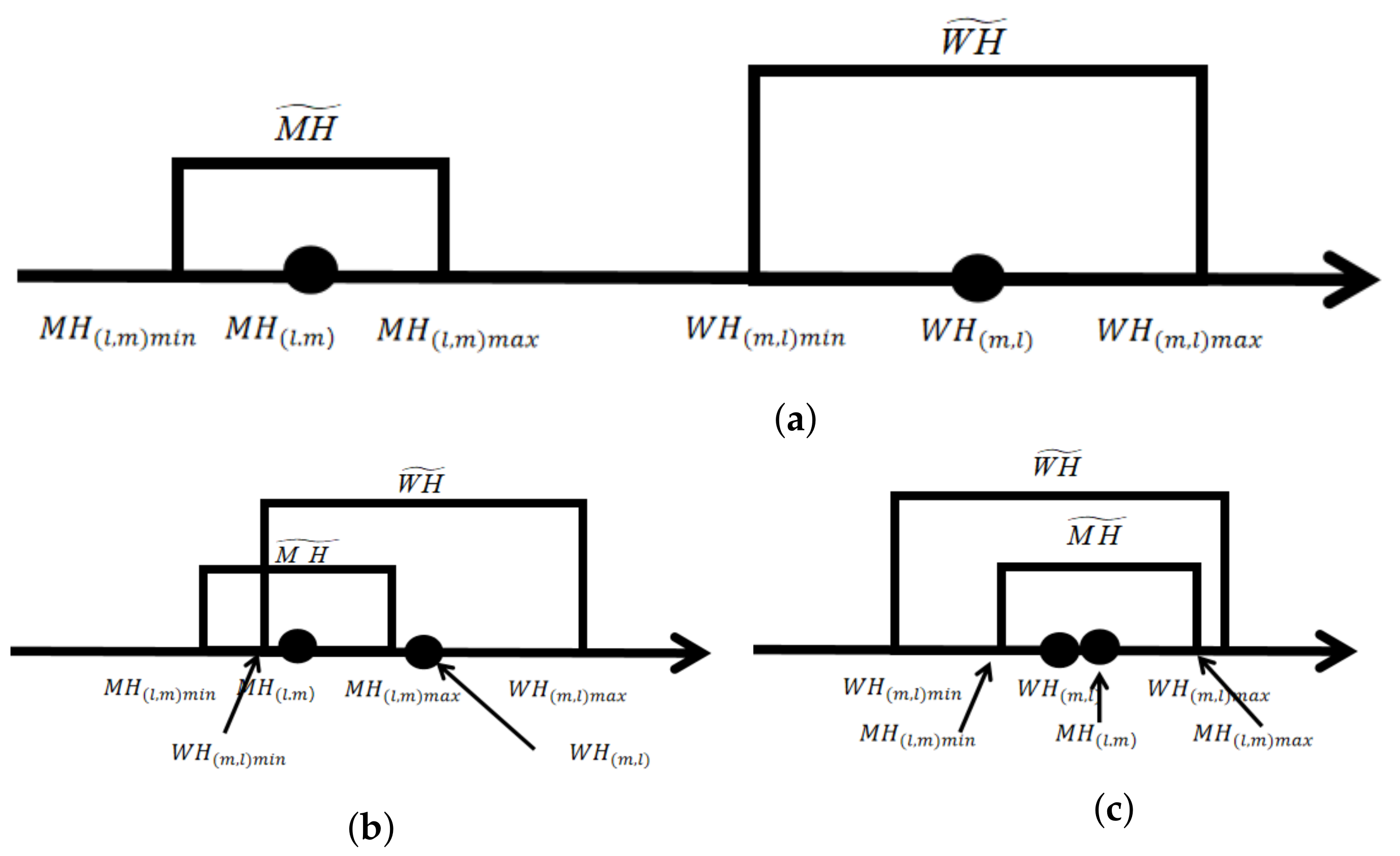
(2). Most of the existing research is carried out under the condition of certain information. However, due to the complexity, concealment and transient nature of the battlefield environment, the information required for most UAV operations is often uncertain. Therefore, in the case of less information, considering the ambiguity of information in the process of UAV coordinated ground attack meets the actual combat needs.
(3). On the other hand, most of the existing research on UAV cooperative ground attack task assignment only focuses on unilateral action strategies, but due to the confrontational nature of the combat environment, it is very applicable to consider the opponent’s possible defense strategies when attacking modeling and analysis through game theory.
(4). For the solution of the Nash equilibrium of the game model, the traditional intelligent optimization algorithm still has the shortcomings of weak global search ability and an easy to fall into local optimum, which urgently needs further optimization.
This article mainly discusses the above four issues, and logically it is a layer-by-layer progressive relationship, as shown in Figure 1, Section 2. The main work of this paper is to conduct multi-attribute evaluation and target strategy selection on the decision-making set through the situation analysis of both parties, and establish the dynamic non-zero and Nash equilibrium maneuver decision-making model of both parties. On the basis of the first section, the second section mainly introduces the improved dynamic non-zero and Nash equilibrium maneuver decision-making model after considering the ambiguity of information in actual combat and the possible defense strategy of the opponent. In the third section, the improved particle swarm optimization algorithm is used to solve the model proposed in the second section. The last section verifies the advantages of this model algorithm over traditional algorithms with a simulation comparison experiment.
Based on the above analysis, this paper aims at the cooperative confrontation problem of UAV clusters. First, under ideal conditions, that is, the information of both sides of the confrontation is completely accurate and known. Through the situation analysis of both sides, the multi-attribute evaluation of the decision set and the selection of target strategies are carried out to establish a dynamic non-cooperative relationship between the two sides. A zero-sum Nash equilibrium maneuver decision model. On this basis, the ideal conditions are modified, that is, considering the actual environment of the battlefield, including the performance difference of the drones of the two sides of the game, it is impossible for us to grasp the accurate information of the opponent in time, and because the radio environment of the battlefield is relatively complex, there may be data errors caused by ground information warfare forces interfering with our information acquisition. This paper improve the dynamic non-zero and Nash equilibrium maneuver decision-making model. Afterwards, through the improved particle swarm optimization algorithm, the efficient calculation of the Nash equilibrium solution of the non-zero-sum game model is realized, and the optimal mixed strategy of both parties is obtained. Finally, the effectiveness of the proposed method is verified by numerical simulation experiments.

2. Mathematical Modeling of Dynamic Non-Zero-Sum Game and Nash Equilibrium Decision-Making under Ideal Conditions

Before discussing the model in this section in detail, the following definitions are given first:
Definition 1.
Non-zero-sum game [26]: Non-zero-sum game is opposite to zero-sum game. A zero-sum game means that the sum of the interests of all players in the game is fixed, that is, if one party gains something, the other party must lose something. A non-zero-sum game means that the sum of the gains of each player under different strategy combinations is an uncertain variable, also known as a variable-sum game.
Definition 2.
Nash Equilibrium [27] (Nash Equilibrium Point): It refers to the non-cooperative game (Non-cooperative game) involving two or more participants, assuming that each participant knows the equilibrium strategy of other participants, a conceptual solution in which no player can benefit himself by changing his strategy.
Definition 3.
The non-zero-sum attack-defense game model (NADG), is a quaternion NADG = {W, M, S, WH}:
W and M are collectively referred to as participants, where W represents the attacker and M represents the defender.
S = { S W , S M } is the strategy set. In this paper, the strategies of all participants are the same, which are maintaining the original flight state, accelerating, decelerating, turning left, turning right, climbing and diving.
WH = { WH W , WH M } is the income function matrix of both attackers and defenders.

2.1. Model Assumptions

(1) Under ideal conditions, it is assumed that both parties can grasp all the complete and accurate information of the other party, and the information is instantaneous, and there is no time difference in the dissemination of information.
(2) Assuming that the objective conditions (including weather, equipment, etc.) are good, the onboard computer can accurately calculate the relevant data based on the global information, and the error is negligible.
(3) Assuming that the UAV cluster flight trajectory is discretized, that is, the confrontation trajectory between the two sides is composed of several maneuvers.

2.2. Set of Maneuvering Strategies for Both Sides of the Game

For dynamic UAV confrontation, the strategy set of dynamic non-zero-sum game Nash equilibrium maneuvering decision needs to be established. The red and blue UAV swarms are named W and M, respectively, where the W UAV swarm consists of p individual UAVs and the M UAV swarm consists of q individual UAVs. In the process of confrontation between the two sides, by assumption (3), their flight trajectories can be considered as a combination of several consecutive maneuvers, which are maintaining the original flight state, accelerating, decelerating, turning left, turning right, climbing, and diving, in order to be recorded as c 1 , c 2 , , c 7 . In summary, the overall strategy set of the drone swarm can be expressed as
S M = S M 1 , S M 2 , , S M 7 S W = S W 1 , S W 2 , , S W 7
where the maneuvering strategy of individual square drones is S W = S M = c 1 , c 2 , , c 7 . Since the strategy number of each individual drone is 7, the strategy numbers of drone group W and drone group M are n W = 7 P and n M = 7 P , respectively.

2.3. Maneuver State Assessment of Both Sides of the Game

In the text, based on the research of Zhang Shuo et al. [28], the situational advantage equation function is used to evaluate and qualitatively describe the state of maneuvering attributes of both players in the game. Assume that in the actual combat process, the maneuver attributes are mainly characterized qualitatively by distance advantage, speed advantage, and angle advantage, and each advantage is characterized by the existing situational advantage equation. By weighting and summing the above three advantages, the dominant state of the UAV group at a certain moment can be obtained.
Record the maneuvering attribute as Q, distance advantage D, speed advantage V, and angle advantage A.
Q = D , V , A
  • Distance advantage
Define M D as the speed advantage of a single existing drone over a single enemy drone:
M D = e ( D R 0 R min R max ) 2
where D is the Euclidean distance between the two sides of the game, R max is the maximum starting distance, R min is the minimum starting distance, R 0 = R min R max / 2 where R max , R min are, respectively, determined by the attribute parameters of the UAVs of both sides of the game.
  • Speed advantage
Define M V as the speed advantage of your own single UAV over the target UAV:
M V = 0.1 0.1 V W i 0.6 V M j , V W i V M j 0.5 0.6 V M j V W i 1.5 V M j , 1 V W i 1.5 V M j .
where V w i is the individual flight speed of W UAV group and V M j is the individual flight speed of M UAV group.
From the above speed advantage function, it can be seen that when the speed V W i of the own drone is greater than 1.5 times the speed V M j of the target drone, the speed advantage M V is the largest.
  • Angle advantage
Define M A as the speed advantage of a single UAV of one’s own side relative to a single UAV of the enemy.
M A = A 1 180 ° A υ 180 ° + 1 2
Among them, A l is the incident angle of the target, and A V is the angle of view of the own side’s single UAV. A l and A V can be calculated from the real-time position, declination angle, pitch angle and other information of both parties. From the above angle advantage function, it can be found that when the target incident angle A l is larger and the viewing angle A V is smaller, the angle advantage M A is greater.

2.4. Establishment of the Overall Dynamics and Payoff Matrix of a Single Game per Unit of Time

2.4.1. Overall Posture Matrix

From Section 2.2, the number of strategies for UAV group W and UAV group M are n W = 7 P and = 7 P , respectively. When W adopts the l ( l = 1 , 2 , , n W ) strategy and M adopts the mth ( m = 1 , 2 , , n W ) strategy, the ith ( i = 1 , 2 , , p ) individual UAV in W has the distance advantage, speed advantage and angle advantage for the jth ( j = 1 , 2 , , q ) individual UAV in M. The distance advantage, speed advantage and angle advantage of the individual UAV are WM D ( i , j ) , WM Y ( i , j ) , WM A ( i , j ) , respectively. The overall posture can be obtained as follows.
WX ( i , j ) = Wk 1 M D ( i , j ) + Wk 2 M V ( i , j ) + Wk 3 M A ( i , j ) i = 1 , 2 , , p , j = 1 , 2 , , q
where Wk 1 Wk 2 Wk 3 are the overall posture weighting parameters, and Wk 1 + Wk 2 + Wk 3 = 1 .
Therefore, the matrix WX is the overall posture matrix of the UAV swarm W when the UAV on the W side adopts the 1st strategy and the UAV on the M side adopts the m strategy.
The matrix WX is the overall posture of W to M. Similarly, the matrix MX can be built in the same steps. jth individual of M ( j = 1 , 2 , , q ) , its distance advantage, speed advantage and angle advantage to ith ( i = 1 , 2 , , p ) individual UAVs of UAV group W are MM D ( i , j ) , MM Y ( i , j ) , MM A ( i , j ) , and the overall posture can be calculated as
MX ( j , i ) = Mk 1 M D ( j , i ) + Mk 2 M V ( j , i ) + Mk 3 M A ( j , i ) i = 1 , 2 , , p , j = 1 , 2 , , q
where Mk 1 Mk 2 Mk 3 are the overall posture weighting parameters, respectively, and Mk 1 + Mk 2 + Mk 3 = 1 .
Therefore, matrix WX is the overall posture matrix of UAV swarm M when UAV on M side adopts the m strategy and UAV on W side adopts the lst strategy. Therefore, the matrix MX is the overall situation matrix for the UAV group M when the M-side UAV adopts the Mth-th strategy and the W-side UAV adopts the lth strategy.

2.4.2. Overall Payoff Matrix

Based on the establishment of the overall situation matrix in the previous section, the income matrices (also called payment matrices) of W and M are, respectively, established according to different strategy sets. In actual scenarios, cluster confrontation strategies can be divided into global confrontation strategies, local confrontation strategies, global penetration strategies and local penetration strategies. The profit matrix under different strategies is different. This article mainly considers the global object, so the following mainly uses W as an example to introduce the establishment process of the profit matrix under the global confrontation strategy and the profit matrix under the global penetration strategy.
(1)
Global confrontation strategy. The main objective of this strategy is to optimize the overall posture of our side, and according to this objective, the gain matrix of W can be obtained:
WH ( l , m ) = 1 pq i = 1 p j = 1 q WX l , m ( i , j ) . l = 1 , 2 , , n W , m = 1 , 2 , , n M .
(2)
Global penetration strategy. The main objective of this strategy is the worst overall posture of the opponent, and according to this objective, the gain matrix of W can be obtained:
WH ( l , m ) = 1 pq i = 1 p j = 1 q MX m , l ( i , j ) . l = 1 , 2 , , n W , m = 1 , 2 , , n M .
Similarly, the payoff matrix of M under different strategies can be built based on the above steps. Similarly, in this paper, only the gain matrices of the global confrontation strategy and the global surprise strategy of M are illustrated.
(3)
Global confrontation strategy. The main objective of this strategy is to optimize the overall posture of our side, and according to this objective, the gain matrix of M can be obtained:
MH ( m , l ) = 1 pq i = 1 p j = 1 q WX l , m ( j , i ) . l = 1 , 2 , , n W , m = 1 , 2 , , n M .
(4)
Global penetration strategy. The main objective of this strategy is the worst overall posture of the opponent, and according to this objective, the gain matrix of M can be obtained:
MH ( m , l ) = 1 pq i = 1 p j = 1 q MX m , l ( j , i ) . l = 1 , 2 , , n W , m = 1 , 2 , , n M .
In summary, the preparation of the mathematical model for dynamic nonzero and Nash equilibrium decision making under ideal conditions is basically completed. Since the model in this section is based on the assumption of ideal conditions, the mathematical model will be improved in the next section of this paper to make it closer to the actual situation, which in turn makes the decision more accurate and informative.

3. Improvement of Mathematical Modeling of Dynamic Non-Zero and Nash Equilibrium Decision Making under Non-Ideal Conditions

3.1. Problem Analysis

3.1.1. Consider the Enemy’s Strategy Choice

Now consider the following situation, when our UAV group adopts two different strategies, A and B, the maneuver advantage over the enemy is 100, and the enemy responds to our A and B with the same maneuver, respectively. In terms of strategy, the maneuvering advantages relative to our side are 60 and 80, respectively. According to the above case analysis, if we adopt different strategies based solely on our maneuvering advantage over the enemy, there is no difference between A and B strategies at this time. But in fact, when strategy A is adopted, the enemy’s threat to our side is relatively small, and our optimal strategy should adopt strategy A. Therefore, based on the simple analysis of the above examples, the own side should consider the enemy’s strategy when making a decision.

3.1.2. Considering the Actual Battlefield Operational Environment

The model in Section 2 is based on two assumptions. However, in actual conditions, due to the performance differences between the UAVs of the two sides of the game, it is impossible to grasp the accurate information of the other side in time, and because of the more complex radio environment on the real field and because the other party may have information jamming technology, there may be errors in the acceptance of the other party information by the UAV of the already side. In summary, the assumptions of model 1 do not meet the actual combat situation and will be improved in this section.

3.2. Model Revision

3.2.1. Model Correction Based on Information Uncertainty

Under the assumptions in the previous section, each element of the gain matrix is a definite value, but in reality, there is a certain error in the transmission and acquisition of information, so there is a certain error in the information received by the UAV. In order to be closer to the actual situation, when calculating the posture value using the dominance function, an error factor (sign) is introduced, and (2) (3) (4) is amended to obtain the following new posture dominance function.
M ˜ D = e D R 0 R max R min 2 α M ˜ D M D min , M D max M D min = M D · α min , M D max = M D · α max
where α is the error factor of distance dominance, M ˜ D is the probability interval information of distance dominance, α min is the lower limit of error, α max is the upper limit of error, M D min is the lower limit of the large probability value of distance dominance, and M D max is the upper limit of the large probability value of distance dominance. The distance dominance accuracy values are taken randomly on this interval and obey uniform distribution.
M ˜ V = M V β M ˜ V M V min , M V max M V min = M V · β min , M V max = M V · β max
where β is the error factor of speed advantage, M ˜ V is the probability interval information of distance advantage, β min is the lower error limit, β max is the upper error limit, M V min is the lower limit of the large probability value of speed advantage, and M V max is the lower limit of the large probability value of speed advantage. The accurate value of speed advantage is taken randomly on this interval and obeys uniform distribution.
M ˜ A = A 1 / 180 ° A υ / 180 ° + 1 / 2 γ M ˜ A M A min , M A max M A min = M A · γ min , M A max = M A · γ max
After the above corrections, a new overall posture dominance function is obtained.
T ˜ = k 1 M ˜ D + k 2 M ˜ V + k 3 M ˜ A
Since M ˜ D , M ˜ V , M ˜ A are all interval numbers, T ˜ is also an interval number.

3.2.2. Non-Zero and Dynamic Nash Equilibrium Decision Model Based on Information Uncertainty

The analysis in this section is based on the assumptions of Section 3.2.1. Due to information uncertainty, each element in the resulting payoff matrix is an interval number, and the matrix WL ˜ is the matrix of the overall posture function when W takes the m strategy and M takes the 1st strategy as follows.
WL ˜ = WL ˜ a 11 WL ˜ a 12 WL ˜ a 1 n WL ˜ a 21 WL ˜ a 22 WL ˜ a 2 n WL ˜ an 1 WL ˜ an 2 WL ˜ apq
= WL min a 11 , WL max a 11 WL min a 12 , WL max a 12 WL min a 1 n , WL max a 1 n WL min a 21 , WL max a 21 WL min a 22 , WL max a 221 WL min a 2 n , WL max a 2 n WL min an n 1 , WL max an 1 WL min an 2 , WL max an 2 WL min ann , WL max apq
The payoff interval matrix is built on the basis of the overall posture matrix, and the specific process is similar to Section 2.4.2 and will not be repeated here, the payoff matrix is as follows.
WH ˜ = WH ˜ a 11 WH ˜ a 12 WH ˜ a 1 n WH ˜ a 21 WH ˜ a 22 WH ˜ a 2 n WH ˜ an 1 WH ˜ an 2 WH ˜ apq
After obtaining the gain interval matrix, based on the consideration of Section 3.2.1, in order to better measure the true posture of the already side’s UAV, not only the gain interval matrix of the already side is needed, but also the gain interval matrix of the opposite side MH ˜ is needed to calculate the gain interval matrix of the enemy, and WH ij and MH ji are analyzed and compared, and the specific analysis and comparison process is as follows: according to the matrix (true value matrix), WH ij can be compared with MH ji in two cases, which are if WH ij is greater than MH ji and WH ij is less than MH ji . If WH ij is greater than MH ji , there are three more cases as follows [3].
Definition 4.
Relative dominance: Assuming that the upper limit of the interval of WH ij ˜ is higher than the upper limit of the interval of MH ij ˜ , there are only three cases: WH ij ˜ and MH ij ˜ have no intersection (Figure 2a), WH ij ˜ and MH ij ˜ have intersection and B is not completely contained in W H ij ˜ (Figure 2b), MH ij ˜ is completely contained in WH ij ˜ (Figure 2c). According to these three situations, this paper defines the result calculated by Equation (19) as the relative dominance of WH ij ˜ to MH ij ˜ .
p WH ˜ ij > MH ˜ ji = 1 , MH ji max WH ij min ; g max 1 g max 2 g max 1 g min 1 + g max 2 g min 1 g max 1 g min 1 · g min 1 g min 2 g max 2 g min 2 + 0.5 g max 2 g min 1 g max 1 g min 1 · g max 2 g min 1 g max 2 g min 2 , MH j i min < WH i j min < MH j i max g max 1 g max 2 g max 1 g min 1 + 0.5 g max 2 g min 2 g max 1 g min 1 , WH ij min MH ji min < MH ji max
Definition 5.
Dominance coefficient, a value measuring the degree of dominance of an existing UAV over an opposing UAV, judged by the degree of relative dominance, calculated as follows.
ψ ij = 1 , 0.9 < H ij < 1 ; 0.9 , 0.6 < H ij < 0.9 ; 0.8 , 0 < H ij < 0.6
According to the definition of the dominance coefficient, if the dominance coefficient is 1, when both sides take the 1st strategy the mth strategy, respectively, under the premise of our dominance, the overall posture of the already side is absolutely dominant relative to the overall posture of the enemy, and the opposite side is less threatening to us when we complete the 1st strategy; if the dominance coefficient is 0.9, it means that the overall posture of the already side is relatively dominant relative to the overall posture of the opposite side, and if the dominance coefficient is 0.8, it means that the overall posture of the opponent is generally superior to the overall posture of the opposite side, and the opponent needs to pay a larger price while completing their tactical moves.
According to Equations (10) and (16), we can obtain the gain interval matrix WH ˜ and MH ˜ for W and M, respectively, after which we can derive the dominance coefficient matrix of the already party’s UAV group W according to Equations (17) and (18). Using the dominance coefficients, the matrix WH can be modified, which in turn yields the matrix WH ^ as follows.
WH ^ = WH ^ 11 WH ^ 12 WH ^ 1 n M WH ^ 21 WH ^ 22 WH ^ 2 n M WH ^ n W 1 WH ^ n W 2 WH ^ n W n M
= WH 11 · ψ 11 WH 12 · ψ 12 WH 1 n M · ψ n M WH 21 · ψ 21 WH 22 · ψ 22 WH 2 n M · ψ 2 n M WH n W 1 · ψ n W 1 WH n W 2 · ψ n W 2 WH n W n M · ψ n W n M
After building the improved payoff matrices WH ^ and WH ^ for W and M, respectively, the confrontation between the two sides of the game is a typical non-zero-sum game due to the different nature and purpose of the drone swarms on both sides of the confrontation
Definition 6
([2]). Mixed strategy Nash equilibrium: Let a non-cooperative game in which there are n insiders involved, where the pure strategy of insider i is denoted as s i = s 1 i , s 2 i , , s m i i and the mixed strategy of i is defined as x i = x i 1 , x i 2 , , x i m i x ij 0 , j = 1 m ij X ij = 1 , i.e., the inning chooses the jth strategy with the probability of x ij . If a mixed strategy combination X = x 1 , x 2 , , x n satisfies μ i X μ i x i , X i ( i = 1 , 2 , , n ) , where μ i denotes the payoff function of i and X i = x 1 , x 2 , , x i 1 , x i + 1 , x n , i.e., a single inning changes its strategy and its payoff value does not increase, then X is said to be the Nash equilibrium of this non-zero-sum game.
From Definition 6, let the pure strategy sets of W and M be S l W S W and S m M S M , respectively, and the probabilities of individual UAVs of the already party to choose the corresponding strategies are x l l = 1 , 2 , n W and y m m = 1 , 2 , n G . In summary, the mixed strategy of W and G can be expressed in the following form.
X = x R n W l = 1 n W x l = 1 , x l > 0 , l = 1 , 2 , , n W Y = x R n M m = 1 n M x l = 1 , x m > 0 , l = 1 , 2 , , n M ,
Based on the characteristics of non-zero-sum games, the following theorems exist.
Theorem 1
([29]). For any mixed strategy ( X , Y ) , there exists a Nash equilibrium solution ( X , Y ) satisfying the following conditions.
X T FHY X T FHY , X T FH T Y X T FH T Y
The Nash equilibrium solution obtained at this point is the optimal strategy of the nonzero-sum game for W and M. In order to quickly solve the Nash equilibrium solution satisfying Equation (15), Equation (15) is transformed into the following optimization problem.
min E X , Y X = x R n F l = 1 n F x l = 1 , x l 0 , l = 1 , 2 , , n F , Y = y R n G m = 1 n G y m = 1 , y m 0 , m = 1 , 2 , , n G ,
E X , Y = max max l = 1 , 2 , n F FH l Y X T FHY , 0 + max max m = 1 , 2 , n G X T GH T X T GH T Y , 0
where the mixed strategy in which the function E ( X , Y ) or E ( X , Y ) takes the minimum value of 0 is the Nash equilibrium point of the original non-zero-sum game problem.

3.3. Dynamic Nash Equilibrium Decision Model

The non-zero-sum game process of W and M within the unit process is given in the first two sections, and in the actual situation, the two drone swarms are a dynamic game process, which is combined via several unit processes, so a dynamic Nash equilibrium decision model is needed. The specific steps of the model are as follows.
(1) Set the simulation parameters and initial conditions according to the actual situation of the UAVs on both sides of the game, and specify the unit step size and the maximum number of iterations.
(2) According to the real-time state parameters of both sides, under the combination of different strategies, the overall state advantage function of individual UAVs is calculated according to Equations (6)–(9), so as to obtain the gain matrix of both sides and finally obtain the single-step non-zero-sum game model.
(3) Calculate the Nash equilibrium solution of the non-zero-sum game according to Equations (15) and (16), and obtain the optimal hybrid strategy of both sides of the single-step game.
(4) Calculating the position and other state parameters of each UAV where it will be located next from the step length specified in step (1).
(5) According to the state parameters calculated in step (4), determine whether the game is over, if the conditions for the game to proceed are still met, return to step (2), if the conditions for the game to end have been met, proceed to step (6).
(6) The game ends, and the results of both sides of the game are derived.

4. Optimization and Solution of Dynamic Nash Equilibrium Strategy

For the intelligent algorithm solution of non-cooperative game model Nash equilibrium, predecessors have carried out a lot of related work. The research results show that the PSO algorithm is excellent in finding Nash equilibrium [30]. Therefore, this paper uses the PSO algorithm to solve the Nash equilibrium. In view of the disadvantages of the classic PSO algorithm, such as premature convergence and low precision, this paper makes certain improvements to the PSO algorithm.

4.1. Classical Particle Swarm Algorithm

Section 3.3 gives the Nash equilibrium maneuver decision model and its solution process for the dynamic non-zero-sum game of cooperative UAV swarm confrontation under asymmetric uncertain information, the core of which is in the solution of the optimization problem Equation (15) with step (3). Therefore, how to find the optimal solution of Equation (15) quickly and efficiently becomes the key to the optimization of dynamic non-zero-sum Nash equilibrium strategies.
In this paper, the search capability of PSO is improved by optimizing the adjustment of inertia weights in it based on the use of the classical particle swarm optimization (PSO) algorithm, which is an optimization algorithm that simulates the foraging process of a flock of birds, where the potential solution of each optimization problem is a bird in the search space, called a particle.
Assuming that the search space is a multidimensional space of D dimensions, the velocity vector and position vector of a particle can be defined as follows, respectively:
X i = x i 1 , x i 2 , , x i D , i = 1 , 2 , , N V i = v i 1 , v i 2 , , v i D , i = 1 , 2 , , N
The equation for its velocity and position update is
υ id = ω υ id + c 1 r 1 p id x id + c 2 r 2 p gd x gd x id = x id + υ id
where c 1 , c 2 are called learning factors, also known as acceleration constants, r 1 , r 2 are random numbers in the range [0, 1], P id is the optimal position searched so far by the ith particle, i.e., the individual extremum, and P gd is the optimal position searched so far by the whole particle population, i.e., the global extremum, and ω is the inertia weight.

4.2. Control of Inertia Weight of Particle Swarm Algorithm

As can be seen from the above equation, the inertia weight controls the influence of the previous variable on the current variable. If ω is larger, it can search the area that the particle failed to reach before, which makes the global search ability of the whole algorithm enhanced, on the contrary, if ω is smaller, the particle mainly searches within the area of the current solution, and the local search ability is enhanced. Therefore, in the field environment, the need to solve the Nash equilibrium solution quickly and accurately is crucial to the field situation, and in the classical PSO, ω is a constant, which cannot adapt to the needs of the solution in different situations, so it needs to be improved.
There are three common methods to improve ω in PSO, adaptive weight method, random weight method and linear decreasing weight method.

4.2.1. Linear Decreasing Method

This method addresses the phenomenon that the PSO algorithm is prone to premature maturity and to oscillation near the global optimal solution at a later stage, even though the inertia weights are decreasing one at a time in accordance with linearity from large to small, and the variation formula is
ω = ω max t × ω max ω min t max
where ω max is the maximum value of inertia weight, ω min is the minimum value of inertia weight, t max is the total number of iteration steps, and t is the number of current iteration 3.

4.2.2. Adaptive Modification Weighting Method

1.
Adjustment according to the distance of global optimum
According to previous studies, the size of the inertia weight is considered to be related to its distance from the global optimum in some papers, and related papers suggest that the inertia weights of different particles proposed in the previous section not only decrease linearly with the increase in the number of iterations, but also decrease with the increase in the distance from the global optimum solution, because the probability of searching for a better solution is greater when the particle is closer to the global optimum solution, so it is necessary to decrease the inertia weight to achieve the purpose of enhancing the local search ability of the particle. In summary, the inertia weights change dynamically depending on the particle positions. And the linear equations generally cannot meet the requirements, so most of them currently use the coefficient formula of nonlinear dynamic inertia weights, which is as follows.
ω = ω min ω max ω min × f f min f avg f min , f f avg ω max , f > f avg
where f is the objective function value of the current step, f avg and f min are the minimum and average values of the objective function values of all particles in the current step, respectively.
As can be seen from the above equation, ω is constantly adjusted as the dispersion of particles changes, and the inertia weight will be reduced when the target value of particles is more dispersed; when the target value of particles is more concentrated, the inertia weight increases.
2.
Adjust the weights according to the degree of early convergence and adaptation value.
The improvement method adjusts its own weights according to the degree of early proficiency of the particle population and the adaptation value of the objective function of each particle, as follows.
ω = ω ω ω min f i f avg f m f avg f m > f i > f avg ω , f m > f i > f avg 1.5 1 1 + k 1 · exp k 2 · Δ , f i > f avg
where f i is the adaptation value of particle p i , and f m is the optimal particle fitness. Then, the average fitness of the particle swarm is f avg = 1 n i = 1 n f i . The particle fitness values that are better than the average fitness values are averaged, denoted as f avg , and define Δ = f m f avg . k 1 , k 2 are called regulation parameters, k 1 is used to regulate the upper limit of ω and k 2 is used to control ω = 1.5 1 1 + k 1 · exp k 2 · Δ of the regulation capacity.
From the definition of Δ , it is known that if the particles in the swarm are too dispersed, Δ becomes larger, thus ω decreases, which enhances the local search ability of the swarm; if the particles in the swarm are too concentrated, Δ becomes smaller, thus ω increases, which enhances the global search ability of the swarm to help jump out the local optimal solution effectively.
In this paper, the adaptive modified weight method is used to improve the PSO algorithm.

5. Simulation Experiments of UAV Cooperative Dynamic Maneuver Decision Algorithm

Based on the UAV cluster adversarial algorithm model based on asymmetric uncertain information environment proposed in the previous two sections, numerical simulation experimental results are presented in this section to verify the validity of the model. The simulation experiments apply the game confrontation steps in Section 3.3, in which the adaptive algorithm in Section 4.2.2 is used to optimize the speed of the algorithm in “calculating the Nash equilibrium solution of the non-zero-sum game and obtaining the optimal hybrid strategy for both sides of the single-step game”.
In order to compare the superiority of the proposed algorithm, W uses the “global adversarial strategy” of the UAV cluster adversarial algorithm based on asymmetric uncertain information environment proposed in this paper, and M uses the classical global adversarial strategy based on the maximum–minimum pure strategy [31]. The following Table 1 shows the initial parameters of the numerical simulation experiment.
Substituting the initial conditions into Equations (3)–(5), we can see that M has a clear advantage in angular posture in the initial stage of the confrontation. In the total 40 steps of the confrontation, they can be roughly divided into “posture equilibrium phase”, “cooperative confrontation phase” and “absolute advantage phase”, and part of the confrontation process is shown in Figure 3, Figure 4, Figure 5, Figure 6, Figure 7 and Figure 8. The red “ Δ ” is the path trajectory position of W at each step, and the blue “*” is the path trajectory position of M at each step. The confrontation ends when one side has an absolute advantage over the other side or reaches the maximum number of confrontation steps.
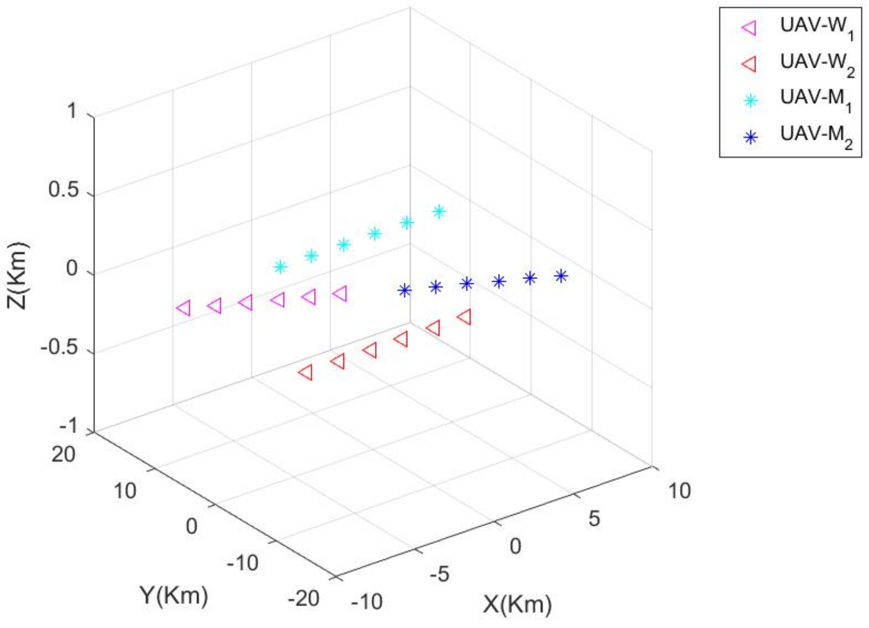
The first stage is the situational balance stage (see Figure 3 and Figure 4). The initial positions of the two sides are far apart. In the fifth step, the two sides enter the opponent’s combat radius, and a confrontation situation occurs. W 1 and M 1 are close to each other and confront each other, and W 2 and M 2 approach each other against each other, as shown in Figure 3.
When the first stage reaches the 10th step, W 1 adjusts the pitch angle by a large margin in order to increase the advantage of the situation, and quickly raises the height of the UAV. Since M 1 is relatively close to W 1 , in order to maintain the overall advantage of M and W, M 1 also quickly adjusts the pitch angle and follows W 1 to reach a higher altitude; while M 2 is responsible for continuing to approach W 2 to expand its own advantages. At this time, due to the hysteresis of the M 1 response, W 1 has a greater advantage over M 1 ; while W 2 is in a tracked state, therefore, M 2 has a greater advantage over W 2 . In the first stage, the two sides have not yet formed a cooperative confrontation, and are still in the stage of balanced confrontation. The confrontation process of step 10 is shown in Figure 3.
The second phase is the postural equilibrium phase (see Figure 5 and Figure 6). At the 14th step, M 2 is still at a disadvantage relative to W 2 , but because M 1 could not form an absolute advantage over W 1 alone due to the large distance and the limitation of the single-step deflection angle change, M 2 gave up the strategy of fighting M 2 alone and makes a strategic adjustment of approaching W 1 and cooperating with M 1 to surround and fight W 1 . And W 2 could not change the direction in time to assist W1 due to the long distance; at this time, M 1 and M 2 as a whole maintain the advantage over W 1 , as shown in Figure 5.
Figure 6 shows the 20th step, W 2 collaborates with W 1 to approach M 2 , at this time W 1 completely removes M 1 , and the M 2 form is intertwined, the advantage of both sides is still not obvious, because the distance W 2 in a shorter number of steps fails to approach M 2 in time, and W 2 together form a pincer attack on M 2 . As shown in Figure 6, at this time, the local gradually forms two against one state, and W’s overall posture advantage gradually forms.
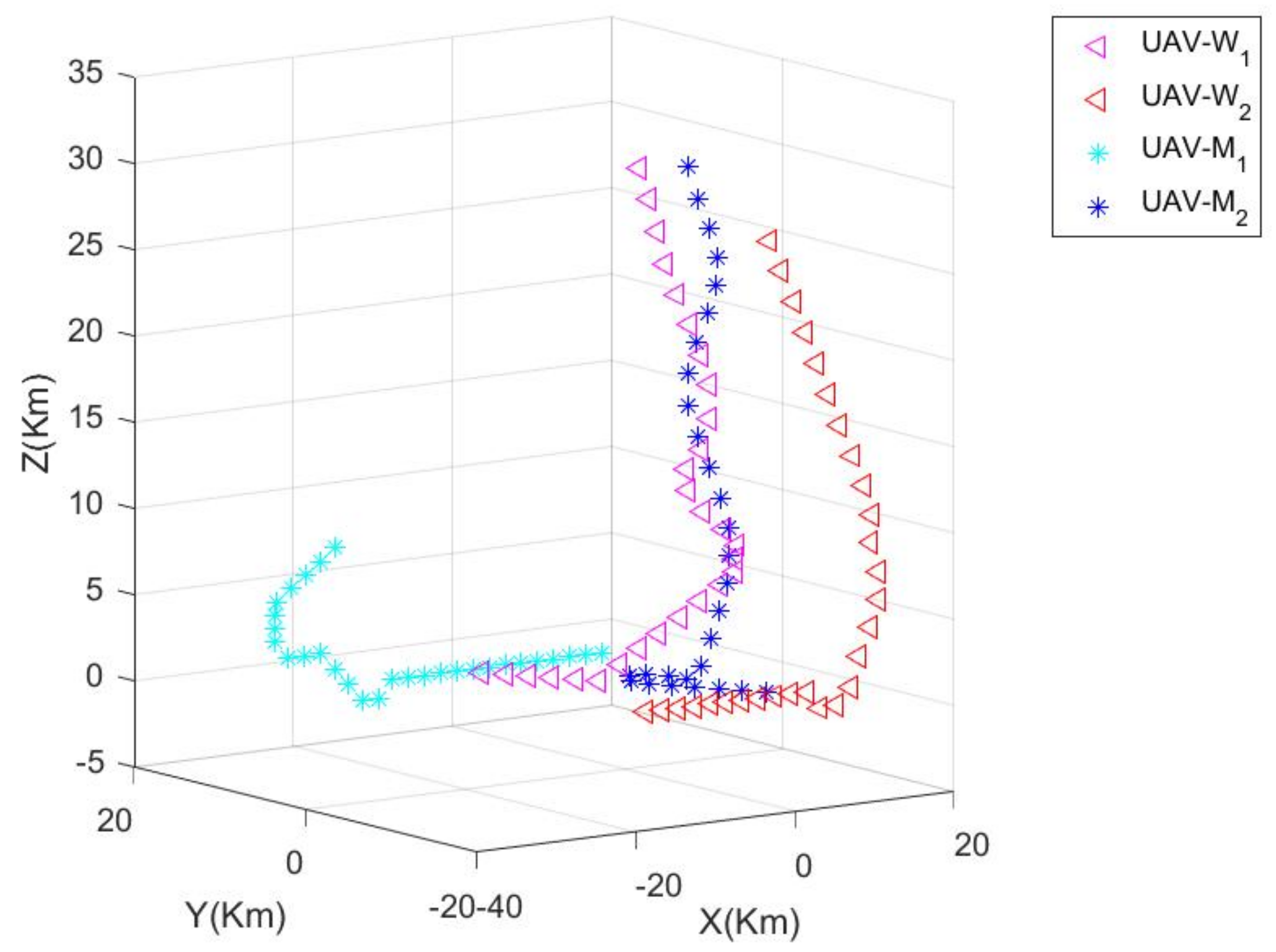
The third phase is the absolute advantage phase (see Figure 7 and Figure 8), in which W maintains the absolute advantage of the overall posture. In step 31 (see Figure 7), W maintains the posture of pinning M 2 , with two chasing one, and the threat to W basically disappears as M 1 maintains a large distance between M 1 and W. W maintains the absolute advantage of the overall posture.
Figure 8 shows the course of the confrontation between the two sides at step 36. In terms of the overall confrontation posture, W maintains the absolute advantage of the overall posture into the third phase. At this point, the confrontation ends.

6. Conclusions

In this paper, a more practical UAV cluster cooperative adversarial decision algorithm based on a dynamic non-zero-sum game under uncertain asymmetric information is proposed based on the actual situation. This article mainly completed the following work:
1. Firstly, based on the actual situation of the actual field, the posture advantage of the adversarial parties under ideal conditions is calculated, and thereafter the gain matrix of the adversarial parties under ideal conditions is further calculated.
2. Secondly, considering the uncertainty of both adversaries in acquiring information and the complexity and variability of the real-time field situation, the information acquired by both adversaries is not the exact value, and the gain matrices of both sides of the game are modified. Then, the particle swarm algorithm is improved to solve the dynamic non-zero and Nash equilibrium maneuver decision model efficiently and quickly to obtain the optimal hybrid strategy based on the actual situation.
3. Finally, a 2-to-2 unmanned cluster cooperative countermeasures simulation experiment is given to verify the superiority and realism of the algorithm proposed in this paper to solve the UAV cooperative countermeasures problem.
Based on the idea of non-zero-sum game, this model regards the solution of Nash equilibrium as the maneuvering action of the UAV cluster. Compared with the traditional model, it has the following advantages:
1. Optimal Strategy: A Nash Equilibrium is an optimal strategy in which each player cannot improve his individual payoff by changing his own strategy given the strategies of the other players. This means that the Nash equilibrium strategy adopted by drone clusters is not easy to be defeated, and it is a relatively stable strategy. It is more suitable for objects such as drones that require high stability.
2. Predictability: Nash equilibrium can be used to predict and understand various game scenarios, especially in complex environments where multiple parties interact. By analyzing and calculating the Nash equilibrium, the drone swarm can speculate on the possible behavior and outcomes of the participants, so as to better predict and plan the strategy of the swarm.
3. Stability: Nash equilibrium is theoretically stable. Even in the face of some disturbances or external pressures, participants will tend to stick to their equilibrium strategies. This stability can help maintain a balanced state of the game and reduce possible conflicts and confrontations. In a more complex actual environment, external disturbances or changes are very frequent. If the UAV cluster changes its strategy too frequently, it will cause damage to itself.
Although this paper has performed some research on the UAV swarm confrontation decision-making problem based on incomplete information, there are still some unresolved problems:
1. In this paper, incomplete information refers to unknowable information such as enemy strategy, enemy revenue, and the partially observable environment when making simultaneous decisions, and does not discuss in depth the unavailable information and untrustworthy information of incomplete information.
2. This paper simplifies the flight process in the UAV swarm air-to-air confrontation environment, and does not take into account the flight characteristics of the UAV itself. In future work, we will focus on a swarm confrontation that is closer to the real environment, including specific attack processes such as missile attacks. In addition, the complex environmental characteristics of the real battlefield have not been fully considered, such as electromagnetic space, weather effects, etc.
3. In the process of UAV swarm confrontation, problems such as large-scale (number greater than 1000) will lead to joint state-action dimensional explosion and dynamic changes in the number of UAVs (scalability) are not considered, which does not meet the requirements of swarm operations actual needs.
To sum up, although this paper has made further research on the basis of existing research, there is still a big gap with the actual environment. The above points will be the key issues of our next research.

Author Contributions

Conceptualization, P.W. and H.W.; Methodology, P.W.; Software, P.W.; Validation, P.W.; Formal analysis, P.W.; Resources, P.W. and P.Z.; Writing—Original draft, P.W.; Writing—review & editing, P.W., H.W., G.L. and P.Z.; Visualization, H.W.; Supervision, G.L.; Funding acquisition, P.W. and P.Z. All authors have read and agreed to the published version of the manuscript.

Funding

Innovation and Entrepreneurship Fund of the Student Work Department of the Party Committee of Northwestern Polytechnical University (NO.2023-CXCY-021), Higher Education Research Fund, Northwestern Polytechnical University (NO.GJJJM202405) and Northwestern Polytechnical University Education and Teaching Reform Research Fund (NO.2023JGZ25).

Data Availability Statement

The data presented in this study are available on request from the corresponding author.

Conflicts of Interest

The authors declare no conflict of interest.

References

  1. Fan, B.; Li, Y.; Zhang, R.; Fu, Q. Review on the technological development and application of UAV systems. Chin. J. Electron. 2020, 29, 199–207. [Google Scholar] [CrossRef]
  2. Wang, Y.; Zhang, W.; Li, Y. An efficient clonal selection algorithm to solve dynamicweapon-target assignment game model in UAV cooperative aerial combat. In Proceedings of the 2016 35th Chinese Control Conference (CCC), Chengdu, China, 27–29 July 2016; pp. 9578–9581. [Google Scholar]
  3. Wang, Y.; Zhao, F.; Wang, H.; Hu, X.; Zhang, W.; Zhang, T.; Feng, Y. Research Status and Development of Graded-index Multimode Fiber Mode-locking Technique. Acta Photonica Sin. 2020, 49, 34–44. [Google Scholar] [CrossRef]
  4. Shao, J.; Xu, Y.; Luo, D. Cooperative combat decision-making research for multi UAVs. Inf. Control 2018, 47, 347–354. [Google Scholar]
  5. Niu, Y.; Xiao, X.; Ke, G. Operation concept and key techniques of unmanned aerial vehicle swarms. Natl. Def. Sci. Technol. 2013, 34, 37–43. [Google Scholar]
  6. Chen, X.; Liu, M.; Hu, Y.-X. Study on UAV Offensive/Defensive Game Strategy Based on Uncertain Information. Acta Armamentarii 2012, 33, 1510. [Google Scholar]
  7. Zhen, Z.; Zhu, P.; Xue, Y.; Ji, Y. Distributed intelligent self-organized mission planning of multi-UAV for dynamic targets cooperative search-attack. Chin. J. Aeronaut. 2019, 32, 2706–2716. [Google Scholar] [CrossRef]
  8. Xu, J.; Guo, Q.; Xiao, L.; Li, Z.; Zhang, G. Autonomous decision-making method for combat mission of UAV based on deep reinforcement learning. In Proceedings of the 2019 IEEE 4th Advanced Information Technology, Electronic and Automation Control Conference (IAEAC), Chengdu, China, 20–22 December 2019; Volume 1, pp. 538–544. [Google Scholar]
  9. Han, Y.; Yan, J.; Chen, R.; Li, J.; Sun, S.; Lin, Y. Improved Game Theory Based Targets Assigning for Ship-based UAV Formation Coordinated Air-to-Sea Attack. Fire Control Command Control 2016, 41, 65–70. [Google Scholar]
  10. Yao, Z.; Li, M.; Chen, Z.; Zhou, R. Mission decision-making method of multi-aircraft cooperatively attacking multi-target based on game theoretic framework. Chin. J. Aeronaut. 2016, 29, 1685–1694. [Google Scholar] [CrossRef] [Green Version]
  11. Zhang, L.; Zhang, A. Study on air formation to ground attack-defends decision-making in uncertainty. Syst. Eng. Electron. 2009, 31, 411–415. [Google Scholar]
  12. Cruz, J.; Simaan, M.A.; Gacic, A.; Liu, Y. Moving horizon Nash strategies for a military air operation. IEEE Trans. Aerosp. Electron. Syst. 2002, 38, 989–999. [Google Scholar] [CrossRef]
  13. Cruz, J.B.; Simaan, M.A.; Gacic, A.; Jiang, H.; Letelliier, B.; Li, M.; Liu, Y. Game-theoretic modeling and control of a military air operation. IEEE Trans. Aerosp. Electron. Syst. 2001, 37, 1393–1405. [Google Scholar] [CrossRef]
  14. Johnson, L.; Ponda, S.; Choi, H.L.; How, J. Asynchronous decentralized task allocation for dynamic environments. In Infotech@ Aerospace 2011; American Institute of Aeronautics and Astronautics (AIAA): St. Louis, MO, USA, 2011; p. 1441. [Google Scholar]
  15. Long, T.; Shen, L.; Zhu, H.; Niu, Y. Distributed task allocation & coordination technique of multiple UCAVs for cooperative tasks. Acta Autom. Sin. 2007, 33, 731. [Google Scholar]
  16. Hu, J.; Wellman, M.P. Multiagent reinforcement learning: Theoretical framework and an algorithm. In Proceedings of the ICML, Madison, WI, USA, 24–27 July 1998; Volume 98, pp. 242–250. [Google Scholar]
  17. Xuan, S.; Zhou, H.; Ke, L. Review of UAV Swarm Confrontation Game. Command Inf. Syst. Technol. 2021, 12, 27–31. [Google Scholar]
  18. Chin, H.H. Knowledge-based system of supermaneuver selection for pilot aiding. J. Aircr. 1989, 26, 1111–1117. [Google Scholar] [CrossRef]
  19. Bechtel, R.J. Air Combat Maneuvering Expert System Trainer; Technical Report; Merit Technology Inc.: Plano, TX, USA, 1992. [Google Scholar]
  20. Bhattacharjee, P.; Rakshit, P.; Goswami, I.; Konar, A.; Nagar, A.K. Multi-robot path-planning using artificial bee colony optimization algorithm. In Proceedings of the 2011 Third World Congress on Nature and Biologically Inspired Computing, Salamanca, Spain, 19–21 October 2011; pp. 219–224. [Google Scholar]
  21. Butenko, S.; Murphey, R.; Pardalos, P.M. Cooperative Control: Models, Applications and Algorithms; Springer Science & Business Media: Amsterdam, The Netherlands, 2013; Volume 1. [Google Scholar]
  22. Lukasik, S.; Zak, S. Firefly algorithm for continuous constrained optimization tasks. In Proceedings of the ICCCI, Wroclaw, Poland, 5–7 October 2009; pp. 97–106. [Google Scholar]
  23. Wu, H.S.; Zhang, F.; Wu, L. New swarm intelligence algorithm-wolf pack algorithm. Syst. Eng. Electron. 2013, 35, 2430–2438. [Google Scholar]
  24. Chen, X.; Li, G.; Zhao, L. Research on UCAV game strategy of cooperative air combat task. Fire Control Command Control 2018, 43, 17–23. [Google Scholar]
  25. Li, B.; Wang, H.; Mu, S. Situation Reasoning Based on Ontology Modeling. Aeronaut. Sci. Technol. 2021, 32, 80–90. [Google Scholar]
  26. Duffy, J. Game Theory and Nash Equilibrium; Lakehead University: Thunder Bay, ON, Canada, 2015; pp. 19–20. [Google Scholar]
  27. Osborne, M.J.; Rubinstein, A. A Course in Game Theory; MIT Press: Cambridge, MA, USA, 1994; p. 14. [Google Scholar]
  28. Liu, K.; Cao, X.; Li, Y.; Fang, D. Research on Cooperative Countermeasures of UAV cluster based on dynamic non-zero-sum game. Aviat. Sci. Technol. 2022, 33, 20–36. [Google Scholar] [CrossRef]
  29. Wang, Y.; Zhang, W.; Fu, L.; Huang, D.G.; Li, Y. Nash equilibrium strategies approach for aerial combat based on elite re-election particle swarm optimization. Control Theory Appl. 2015, 32, 857–865. [Google Scholar]
  30. Pavlidis, N.G.; Parsopoulos, K.E.; Vrahatis, M.N. Computing nash equilibria through computational intelligence methods. J. Comput. Appl. Math. 2005, 1, 113–136. [Google Scholar] [CrossRef]
  31. Muhammad, R.; Saeed, M.; Ali, B.; Ahmad, N.; Ali, L.; Abdal, S. Application of Interval Valued Fuzzy Soft Max-Min Decision Making Method. Int. J. Math. Res. 2020, 9, 11–19. [Google Scholar]
Figure 1. The system architecture of the article.
Aerospace 10 00711 g001
Figure 2. Three situations of interval MH relative to interval WH . (ac) see Definition 4.
Aerospace 10 00711 g002
Figure 3. Simulation of UAV cooperative dynamic maneuvering decision algorithm (step 5).
Aerospace 10 00711 g003
Figure 4. Simulation of UAV cooperative dynamic maneuvering decision algorithm (step 10).
Aerospace 10 00711 g004
Figure 5. Simulation of UAV cooperative dynamic maneuvering decision algorithm (step 14).
Aerospace 10 00711 g005
Figure 6. Simulation of UAV cooperative dynamic maneuvering decision algorithm (step 20).
Aerospace 10 00711 g006
Figure 7. Simulation of UAV cooperative dynamic maneuvering decision algorithm (step 31).
Aerospace 10 00711 g007
Figure 8. Simulation of UAV cooperative dynamic maneuvering decision algorithm (step 36).
Aerospace 10 00711 g008
Table 1. Numerical experiments against double-fire initial basic parameters.
Parameters
Drone Number
W1W2M1M2
Initial location(−400 m, 0 m, 1000 m)(−400 m, 200 m, 1000 m)(400 m, 0 m, 1000 m)(400 m, 200 m, 1000 m)
Initial speed200 m/s200 m/s200 m/s200 m/s
Initial deflection angle60°60°−118°−118°
Initial pitch angle
Time per unitAcceleration60 m/s60 m/s
Deceleration60 m/s60 m/s
Maximum deflection
angle variable
30°30°
Maximum pitch
angle variable
10°10°
Overall situational weighting parameters Wk 1 = 0.3 , Wk 2 = 0.2 , Wk 3 = 0.5 Wk 1 = 0.3 , Wk 2 = 0.2 , Wk 3 = 0.5
Confrontation step limit40 step
Unit decision time1 s
Disclaimer/Publisher’s Note: The statements, opinions and data contained in all publications are solely those of the individual author(s) and contributor(s) and not of MDPI and/or the editor(s). MDPI and/or the editor(s) disclaim responsibility for any injury to people or property resulting from any ideas, methods, instructions or products referred to in the content.

