Article

Observability-Driven Path Planning Design for Securing Three-Dimensional Navigation Performance of LiDAR SLAM

1
Department of Aerospace Information Engineering, Konkuk University, Seoul 05029, Republic of Korea
2
Department of Mechanical and Aerospace Engineering, Konkuk University, Seoul 05029, Republic of Korea
*
Author to whom correspondence should be addressed.
Aerospace 2023, 10(5), 492; https://doi.org/10.3390/aerospace10050492
Submission received: 29 March 2023 / Revised: 13 May 2023 / Accepted: 19 May 2023 / Published: 22 May 2023

Abstract

:
This paper presents an efficient method for securing navigation performance by suppressing divergence risk of LiDAR SLAM through a newly proposed geometric observability analysis in a three-dimensional point cloud map. For this, observability characteristics are introduced that quantitatively evaluate the quality of the geometric distribution of the features. To be specific, this study adapts a 3D geometric observability matrix and the associated condition number for developing numerical benefit. In an extensive application, we implemented path planning in which the enhanced SLAM performs smoothly based on the proposed method. Finally, to validate the performance of the proposed algorithm, a simulation study was performed using the high-fidelity Gazebo simulator, where the path planning strategy of a drone depending on navigation quality is demonstrated. Additionally, an indoor autonomous vehicle experimental result is presented to support the effectiveness of the proposed algorithm.

1. Introduction

For the last decade, demand for automation has strongly increased due to rising labor costs and the non-face-to-face social environment. Autonomous driving technology has become a representative elementary technology for implementing such automation, and therefore, the importance of autonomous driving as a key component to realize indoor and outdoor vehicle missions, such as with delivery robots or serving robots in restaurants, is increasingly emphasized. Specifically, navigation technology that can provide the exact information about positioning and attitude determination is essential for autonomous driving technology. In particular, among technologies related to navigation, SLAM is being extensively deployed in many application fields due to advancements in sensor and data processing technology.
Since SLAM is fundamentally a technology that simultaneously performs precise map generation and relative localization based on the generated map, LiDAR and cameras are widely used to obtain measurement values for environmental map construction. In SLAM implementation, either 2D LiDAR or 3D LiDAR can be selectively used depending on the application purpose and hardware platform. For instance, 2D LiDAR has the advantage that real-time processing is possible even in a low-performance processor as the amount of data is relatively small. However, it is challenging to adopt it in a 6-DOF environment. Vehicles that operate on a flat surface, such as robot cleaners or serving robots, are typical applications. Comparatively, 3D LiDAR can be effectively used in 6-DOF pose estimation problem, yet it requires extensive resources due to its real-time and optimizing computation process based on a vast number of point cloud measurements. In contrast, VIO technology using cameras is known for its relatively low-cost sensors and significant performance improvements based on the wide algorithm deployment and applications in robot vision technology. However, it has limitations such as the inability to provide depth information with a single sensor, vulnerability to optical changes, and decreased performance in environments with insufficient feature point tracking.
SLAM technologies using LIDAR and cameras have developed competitively based on their unique characteristics, but recently, convergence research is being conducted in a way that complements and combines the heterogeneous characteristics of these sensors. In general, it is known that the proposed LVIOs (LiDAR/visual inertial odometry) have a smaller estimation error than the existing LIOs and VIOs [1,2]. For instance, LVI-SAM [1] presents an improved position and attitude estimation accuracy using a LiDAR, camera, and IMU sensors. In this design, VIO (visual inertial odometry) and LIO (LiDAR inertial odometry) form the underlying subsystems, utilizing open-source software such as VINS-Mono [3] and LIO-SAM [4]. When a failure is detected in one of the two subsystems, the system decides to operate independently. If both see sufficient features, the combined mode operates, where VIO selectively extracts depth information from features measured by LiDAR. LIO uses VIO’s odometry information when initial estimation for LiDAR scan-matching is activated. However, this imposes a significant computational burden as simultaneous point cloud processing tasks are associated with each algorithm implementation. FAST-LIVO [2] uses a single-system state matrix to estimate the state and resolve these issues. In detail, the LIO of this SLAM is based on Fast-LIO2 [5], while VIO employs an in-house algorithm based on SVO [6]. For implementation, its VIO utilizes map information from LIO and combines LiDAR data with the measurement level during visual feature extraction. In particular, Fast-LIVO eliminates the extraction and matching stage that takes a significant amount of time, and thus pose can be estimated quickly in the suggested direct integration scheme. However, this approach essentially relies on the quality of state initialization.
SLAM technology, by its very nature, is a method of solving numerical optimization problems by using a local feature map at each instance, where inevitably, pose estimation errors gradually diverge. As a result, errors in the pose estimation accumulate and propagate to distort the exploration map from the true environmental map. Several methods have been suggested to address this issue. The well-known loop closure technique is a representative approach that corrects the accumulated error when revisiting a location marked in the past trajectory. While loop closure was initially developed to improve the estimation performance of SLAM, it has also been expanded to mission-combined tasks such as Active SLAM [7].
Active SLAM research suggests suppressing error divergence by adding route points for loop closing during route planning. This representative research case allows the linking of mission planning with navigation stability in the autonomous exploration of unknown regions. The authors of [8] present a route plan for loop closing in an occupancy grid map. This paper proposes D* using negative edge weights for shortest-path planning. Through this method, the robot improves the error of position estimation while searching. Paper [9] deals with the exploration method of autonomous underwater vehicles in a 3D environment. The authors propose an algorithm for determining the next search point using a joint map and state entropy. In both articles, path planning is performed while estimation error is suppressed to avoid navigation divergence. It is clear that path planning techniques coupled with loop closure to prevent navigation divergence have the disadvantage of degraded performance compared with existing optimized path planning techniques based on objective cost functions.
Despite differences in their measurement data, LiDAR SLAM and vision SLAM have fundamentally similar mechanisms, i.e., creating a local map and estimating the position and attitude through feature registration with the global map. Therefore, position and attitude estimation cannot be performed if feature tracking or map matching fails. One of the cases where matching fails is high maneuverability or fast movement. If the sensor field of view deviates from the local feature point map of the previous epoch, there is no matching part between the map and the sensor data and pose estimation becomes impossible. Another case is when features cannot be extracted from the onboard sensor value. Cases in which feature points cannot be extracted may vary depending on the type and characteristics of the sensor. In the case of image sensors, this occurs when targets are indistinguishable from the background color or images are contaminated by light scattering, for example. In contrast, in the case of LIDAR, feature tracking quality is highly affected by the completeness of point cloud data, which is determined by limitations in the effective measurement distance or precision of the adopted sensor.
SLAM feature quality cannot be guaranteed in situations where there are environmental peculiarities. For example, artificial environments such as buildings and roads are fundamentally composed of many straight lines. Generally, lines can better represent the geometric information of space than points, thus papers [10,11,12] perform SLAM by extracting line features. Furthermore, the authors of [13] perform SLAM using plane features extracted in indoor environments as geometric information about surfaces, and the proposed method takes into account the detection of plane objects of various shapes and sizes for achieving performance. The extraction of geometric objects such as lines and planes is less affected by dynamic obstacles, enabling estimation of position and attitude with relatively high stability and accuracy. However, even these line-based techniques cannot guarantee performance in environments where the same type of geometric structure, such as in corridors or tunnels without obstacles, is repeated. In [14], a special marker called the ArUco is employed to overcome pose divergence in such monotonous flying environments. This marker is uniquely fixed to the reference coordinate system and thus can provide the relative pose between the marker and the vehicle in the factor graphed ArUco-LiDAR navigation system. However, this approach requires burdensome preliminary installation of a global marker with high accuracy. Considering another aspect, the authors of [15] investigated the structural impact of the navigation environment on the estimation performance. Specifically, they analyzed the observability of a navigation system in an environment where geometric features such as points, lines, and planes can be measured by sensors. In [15], simulation studies demonstrated the directions in which each feature cannot be observed and based on this, presented quantitative error analysis results for the area of reduced observability. However, the approach has limitations in that it is not extended to path planning and navigation stability as attempted in Active SLAM, and there was no experimental verification of the proposed algorithm.
Accordingly, this paper proposes a method for securing navigation performance in drone exploration missions that considers the limited field of view (FOV), detection distance, and loadability characteristics of LiDAR, and suggests an algorithm for such missions. Notably, the proposed analysis method suggests applying measurement observability under the geometric variation of explored environments. To achieve this, the paper attempts to identify in advance the environments in which matching is complex. In the 3D point cloud map, the vehicle’s specific location is predicted and used for analyzing its 3D geometric structure. Specifically, this paper proposes using geometric observability and condition numbers in the 3D point cloud map. Thereby, the location where LiDAR SLAM becomes vulnerable is determined in advance. Consequently, the projected location is reflected in the route planning algorithm to secure a successful mission, where the navigation performance is guaranteed during the planned mission trajectories.

2. Observability Analysis

LiDAR SLAM typically uses matching algorithms such as NDT or ICP to estimate the position and map [16,17]. For the point cloud registration, a characteristic shape or topography is mostly required. This implies, in turn, that SLAM performance degrades essentially when the matching is difficult when operating in places such as corridors and tunnels. To overcome this limitation, we propose an observability analysis of LiDAR measurements via the geometric topography. The analysis incorporates the rank and condition number from the induced observability model. Based on this, the divergence tendency of SLAM’s estimate at a predicted position can be evaluated and employed in designing a refined path.

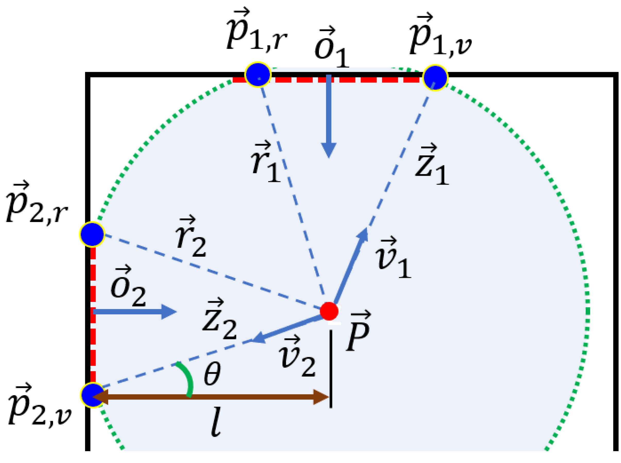
2.1. Observability Model

In this paper, the observation matrix is closely related to LiDAR SLAM realization according to the surrounding terrain at a specific position. LiDAR measurement data are affected by the pose of the vehicle; therefore, position, velocity, and attitude are first defined as the states for observability analysis. In this regard, the states and measurements are organized as in the following way:
X = P n V n Φ b ,   Z = z 1 z 2 m × 1
The measurement is defined in the relationship between the wall and a specific position P. Therefore, the size of the measurement matrix usually increases with the number of walls [18].
Figure 1 is a schematic diagram of the method for finding the geometrical characteristics of the surrounding objects measured through LiDAR at a specific location  P . The measurement Z is obtained according to the geometric relationship between a specific position  P  and the surrounding planes. Observability is analyzed with an orthogonal vector  o i  and two points  p i , r  and  p i , v  on the wall measured at a specific position  P r i  is the relative distance between a specific position  P  and the point  p i , v  on the wall.  v i  is the relative direction vector between a specific position  P  and another point on the wall  p i , v .
r i = p i , r P
v i = p i , v P p i , v P
l  is the vertical distance from the wall to a specific location  P . Thus, the measurement at  P  is expressed as:
z i = l cos θ = o i · r i o i · v i
Next, to derive the observability model, the Lie derivative is to adapted to determine observability in the 3D search domain [19]. Assuming there is one wall surrounding the vehicle, the Lie derivative matrix is given as:
O i = o i T o i T · v i 0 1 × 3 o i T · r i o i T · v i 2 · α i 0 1 × 3 o i T o i T · v i o i T · V o i T · v i 2 · α i 0 3 × 3 0 3 × 3 o i T · r i o i T · v i 2 · α i ×
where
α i = o i T · v i ×
Note that Equation (5) is the observability matrix for one wall. For this system to be observable, a full rank (i.e., rank = 9) is required. When one wall is detected, the rank increases by 1 in each position and velocity, and increases by 2 in attitude. In the multiple wall detection case, rank increases along each wall’s orthogonal vector direction x, y, and z-axis. Equation (7) presents the accumulated observability matrix for multiple walls detection.
O = o 1 T o 1 T · v 1 0 1 × 3 o 1 T · r 1 o 1 T · v 1 2 · α 1 o 2 T o 2 T · v 2 0 1 × 3 o 2 T · r 2 o 2 T · v 2 2 · α 2   0 1 × 3 o 1 T o 1 T · v 1 o 1 T · V o 1 T · v 1 2 · α 1 0 1 × 3 o 2 T o 2 T · v 2 o 2 T · V o 2 T · v 2 2 · α 2 0 3 × 3 0 3 × 3 o 1 T · r 1 o 1 T · v 1 2 · α 1 × 0 3 × 3 0 3 × 3 o 2 T · r 2 o 2 T · v 2 2 · α 2 ×  
The observability matrix is constructed with a size (5 × i) × 9 when there are i walls. The system proves observable when detecting two vertical walls and at least one top or bottom plane. However, in some cases, full rank can be satisfied even with only one horizontal plane and one wall. To avoid this kind of weak observability status, the sensitivity of the matrix is further identified by defining the condition number as below:
κ O = δ m a x O / δ m i n O  
where  δ m a x O  and  δ m i n O  are the maximum and minimum singular values of the observability matrix, respectively. By dividing these two singular values, the observability matrix’s condition number can be obtained as defined in Equation (8). The smaller the value of the condition number, the stronger the independence of each row and column, and thus, the more robust the singularity of the matrix [20,21]. In our approach, the degree of local observability is also measured by the condition number in Equation (8) for the derived observability matrix.

2.2. Geometric Detection

In this section, we present a topological illustration of point cloud data considering the geometric relationship between the predicted vehicle pose information and the surrounding walls in a map. First, at each epoch, the position, velocity, and attitude need to be computed to fix the geometry against the planes within a map and thus construct an observability matrix. Assuming the position is allocated in advance via virtual planning, the rest state can be predicted through the vehicle’s dynamics control result.
Figure 2 shows the sequential steps to obtain the state prediction for a given target position. The position control block implements a PID algorithm, which receives  P c  and outputs the control speed  V c P c  is the difference between the specific position  P  and the previous specific position. Then, the velocity control block receives the control velocity  V c  and outputs the control acceleration  A c . Finally, the quaternion attitude  Q c  is computed by using the desired yaw  ψ  and control acceleration  A c .
For a given vehicle’s pose prediction, geometric observability analysis requires topography such as walls, ceilings, and floors, and classification of the topography needs to be realized around a specific point in 3D point cloud map data. To this end, a point cloud within the sensor range of a specific location is extracted from the 3D point cloud map. These extracted points are processed once again considering the attitude of the vehicle and the field of view of the adopted LiDAR. In this way, the walls can be found in the processing data. Figure 3 shows an exemplary point cloud generation with surrounding wall based on the suggested mechanism.
The technique for finding the wall is based on the split and merge algorithm. The split and merge algorithm calculates the vertical distance of all points on the line connecting the first and last points. If the point with the farthest vertical distance is larger than a threshold, the line is divided around this point. By repeating this process, the line fitting is performed. The lines created at this time are considered as formally separated but virtually connected lines, where straight wall can be piece-wise distinguished for efficiency. The distance between each point is calculated, and the connection is disconnected when the distance exceeds a certain length. The middle point of the line is put into the normal estimation function of the PCL (point cloud library) to calculate the wall’s normal vector. In addition, the normal vector is calculated by extracting the floor surface from previously processed data to match the sensor’s measurement data [22]. Note that this normal vector is used as orthogonal vector  o i  in Figure 1 and serves an essential role in the observability analysis.
In the subsequent sections, two results are demonstrated for verifying the proposed concept. First, the effectiveness of the proposed observability criteria in complex environment is validated, and then the associated path planning performance will be addressed.

3. Observability Verification Study

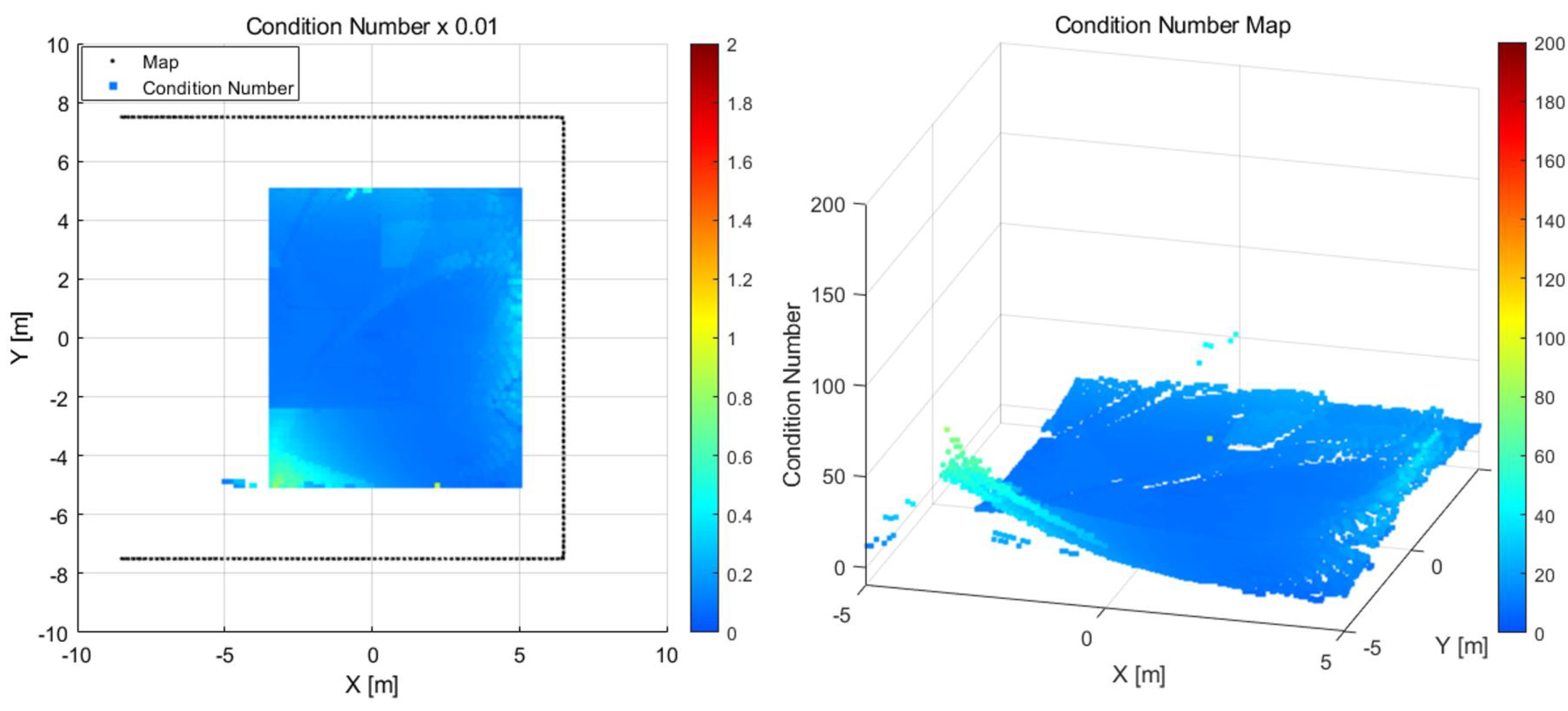
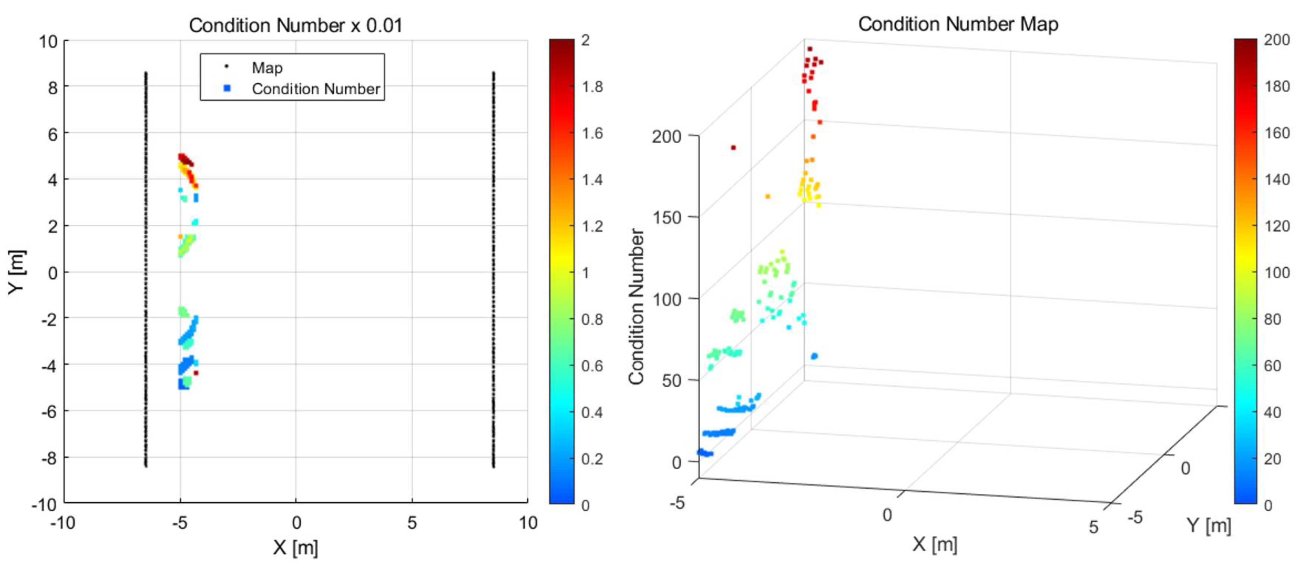
3.1. Simulation Results

For algorithm verification, a virtual environment was configured and tested in Gazebo. Gazebo is a 3D simulation program for robots and uses a physics engine similar to reality, where drone movements or algorithms can be verified in a virtual environment. It also generates and outputs various sensor data such as IMU, LiDAR, and camera data [23]. In Gazebo, sensor data are obtained by simulating the IMU and Ouster’s OS0-32 LiDAR used in the experiments. The SLAM algorithm obtained a point cloud map using LIO-SAM, which is a graph-based SLAM using LiDAR and IMU. When creating a map, a 3D point cloud map is created by extracting the surface and edge of the features, with which the density of the map can be adjusted [4].
In the simulation, there was a complex indoor environment with a number of walls and ceilings. Depending on the environment, the condition number of the observability can vary drastically. The maximum distance of the LiDAR was set to a radius of 10 m.
The first environment was inside a 15 m × 15 m room closed on four sides, as shown in Figure 4. Observability condition numbers were calculated at intervals of 0.1 m for a 10 m × 10 m area from the center of the room. The simulation result was full rank in all areas calculated, and the condition number was calculated to have a value of 80 or less. This means that navigation can be performed well in all areas with LiDAR measurements.
The second case was an environment where three sides are closed, with one open side, as shown in Figure 5. As in the previous experiment, condition numbers were calculated at 0.1 m intervals for a 10 m × 10 m area. From the simulation results in Figure 5, it can be seen that the area close to the open surface was not calculated. In that area, the wall on the left was not measured due to the LiDAR max range. This phenomenon occurs when the rank is seven because the orthogonal vector of the wall is not found in the x-axis direction. Since it is not full rank, it is impossible to calculate the condition number. This means that the features cannot be found in the x-axis direction. There is a high possibility that SLAM will diverge in that region.
The third case was a corridor wall environment with an open top and bottom, as shown in Figure 6. The experimental conditions were the same as in the previous experiment. It can be observed that in almost all areas, the condition number was not calculated. In some places, condition numbers were computed. However, since the values were too large, this rather degrades the performance of the SLAM result. For a comprehensive test based on the above observation, a simulation was performed in the complex maze environment shown in Figure 7.
For the observability analysis, three paths were prepared, as shown in Figure 7a. The environment was composed of a path with no obstacles, a path with complex obstacles, and a path with simple obstacles. The maximum distance of LiDAR was also set to a radius of 15 m. In Figure 7b, it can be observed that a full rank was mostly maintained around the corridor area with detection of obstacles (i.e., middle corridor). The condition number was also calculated to provide relatively low values through the corridor. However, in areas without a detected target (e.g., upper and lower corridor), it was observed that the condition number remained high irrespective of full rank condition. In addition, it can be observed that the condition number contour was closely related to the measurement reachability against the detected walls.

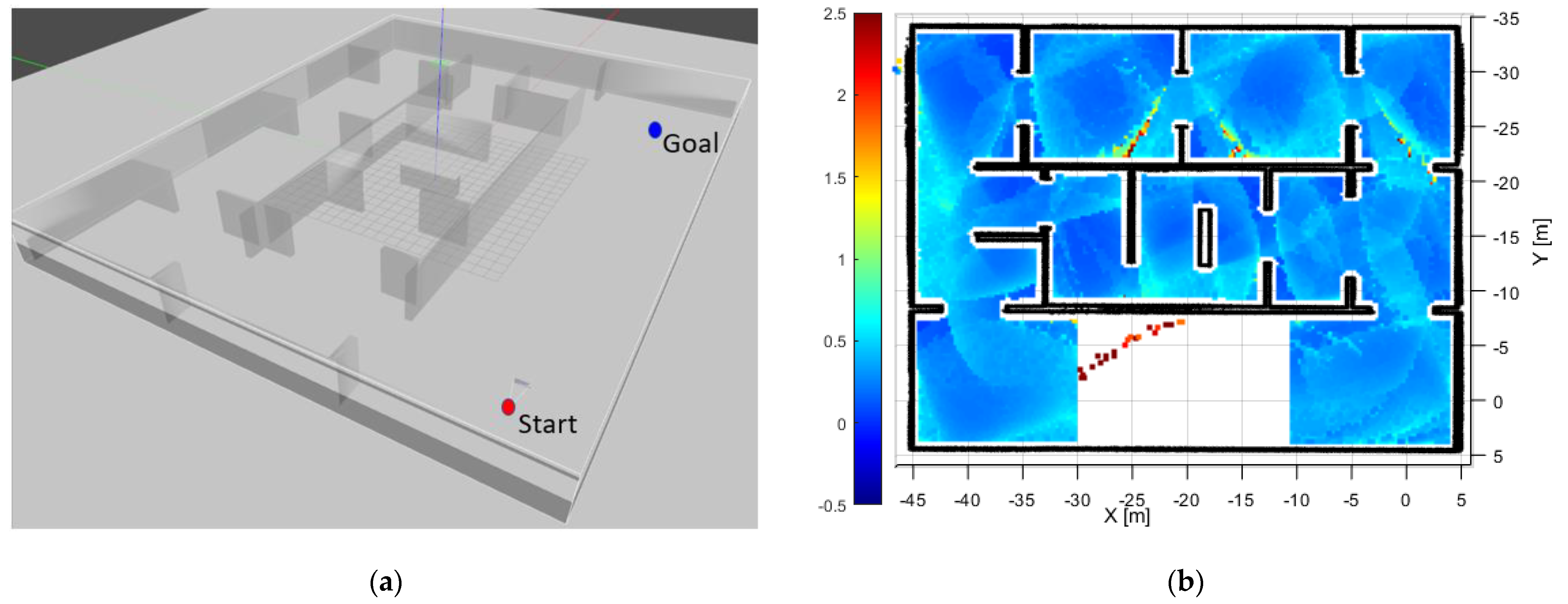
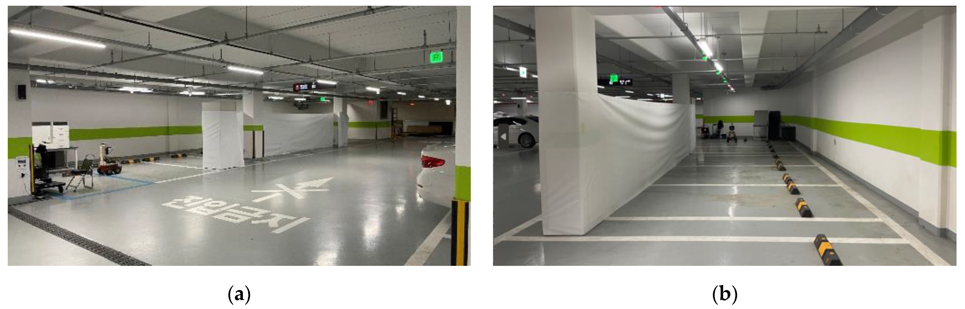
3.2. Results for the Real Environment

A similar map configuration was applied to an experimental environment for performance verification. The place is an underground parking lot with columns at even intervals and an environment with some parked cars. A point cloud map of the parking lot was first acquired through SLAM. The observability and condition number was calculated at 0.1 m intervals in the map.
In Figure 8, it is illustrated how the condition number map changes depending on the detecting distance of LiDAR. The maximum distance of LiDAR was set to 5 m, 7.5 m, 10 m and 20 m, respectively, as shown in the figure. It is observed the result is poor at a shorter maximum distance of LiDAR because the walls were rarely measured. Especially in case of 5 m, in almost all locations, the wall was not measured correctly. Therefore, it can be confirmed that there are many locations where the condition number has not been calculated because full rank condition was not satisfied. In the case of 20 m distance, it was observed that full rank was mostly established where the condition number remained low by recognizing the walls sufficiently at each location.

4. Observability-Driven Path Planning

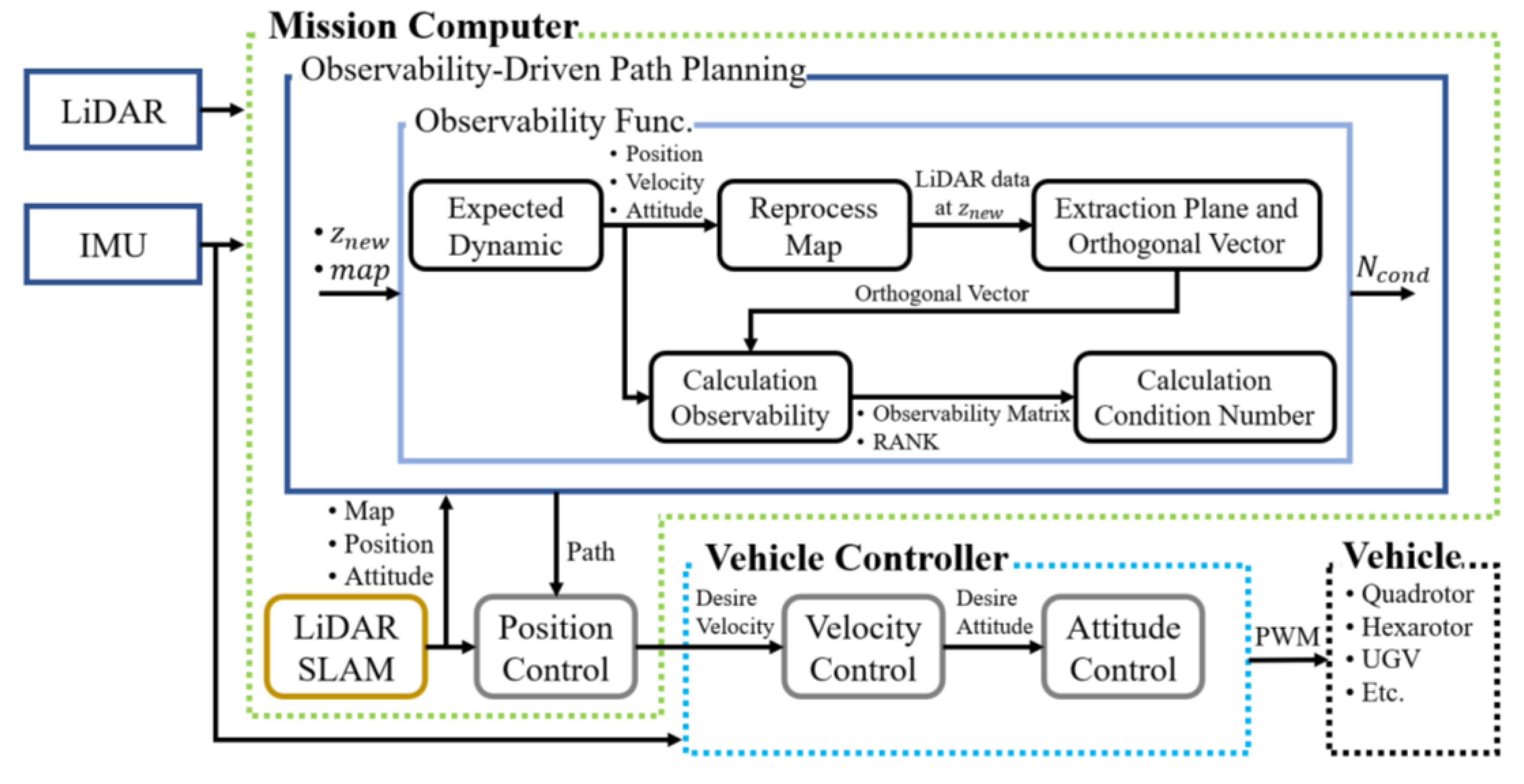
4.1. Algorithm Implementation

Based on the results in Section 3, the pose estimation reliability of SLAM was quantitatively evaluated for further mission application. Naturally, this can be applied to a path planning problem of a robot or drone so that it is possible to reach the destination by avoiding the divergence risk during navigation. In this context, this section proposes to design a path planning strategy by applying the geometric observability analysis technique to RRT* [24].
Fundamentally, the observability-driven path planning technique introduces an observability index into the obstacle collision determination step of the existing RRT*. When creating a path, if an obstacle exists or the condition number is not good, the node at the corresponding location is removed. Through this, a randomly generated branch node is created as a candidate region capable of improving observability quality. Therefore, it has a feature capable of guaranteeing navigation performance when the entire route is constructed to satisfy the criterion.
The pseudo-code of the observability-driven path planning algorithm is summarized in Algorithm 1. In the algorithm, the function at each step is described in detail as follows.
Algorithm 1 Observability-Driven Path Planning.
1:
τ I n i t i a l i z e   T r e e
2:
τ I n s e r t N o d e ,   z i n i t , τ
3:
M o c t o ,   S M a p C o n v
4:
f o r   i = 1   t o   i = N   d o
5:
z r a n d S a m p l e i ,   S
6:
z n e a r e s t N e a r e s t τ , z r a n d
7:
z n e w S t e e r z n e a r e s t , z r a n d
8:
N c o n d O b s e r v a b i l i t y M o c t o , z n e w
9:
i f   1 N c o n d N m a x T h e n
10:
Z n e a r N e a r τ , z n e w , r
11:
z m i n C h o o s e P a r e n t Z n e a r ,   z n e w ,   z n e a r e s t
12:
τ I n s e r t N o d e z m i n ,   z n e w , τ
13:
τ R e w i r e τ , Z n e a r ,   z m i n ,   z n e w
14:
e n d   i f
15:
e n d   f o r
16:
r e t u r n   τ
  • MapConv: This function receives a point cloud map from SLAM and returns Octomap  M o c t o  and map size S. Octomap is an Octree-based map with substantial advantages of fast search and efficient memory management. The reason for converting to Octomap is for the walls search algorithm before observability calculation.
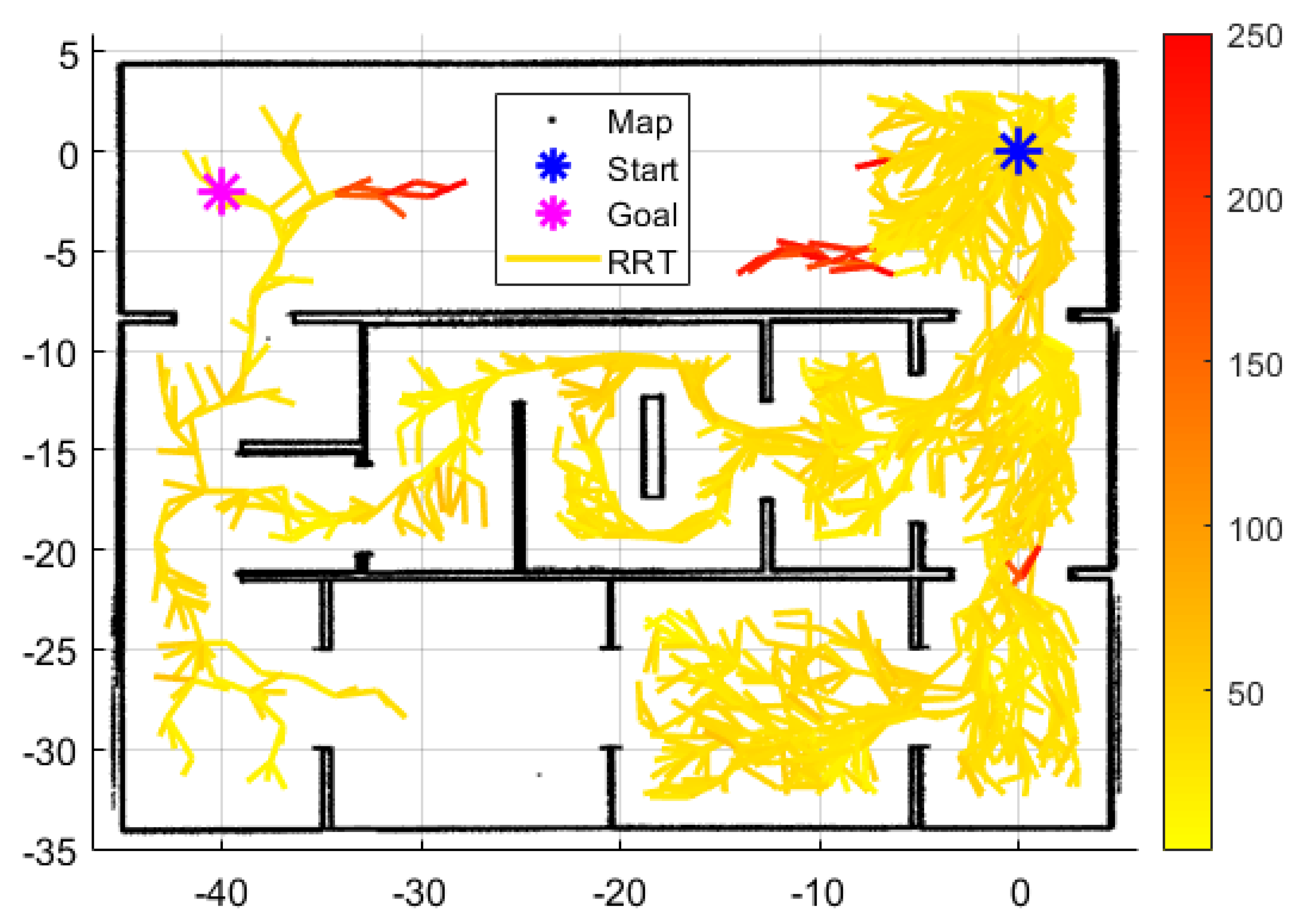
  • Sample: Returns a random position  z r a n d  in map size S.
  • Nearest: Among the nodes of the path tree τ, the node  z n e a r e s t  closest to  z r a n d  is searched and returned.
  • Steer: Calculates the distance and direction between  z n e a r e s t  and  z r a n d . If the distance exceeds a certain distance, a new node location  z n e w  is created at a limited distance in the direction calculated with  z n e a r e s t  as the center.
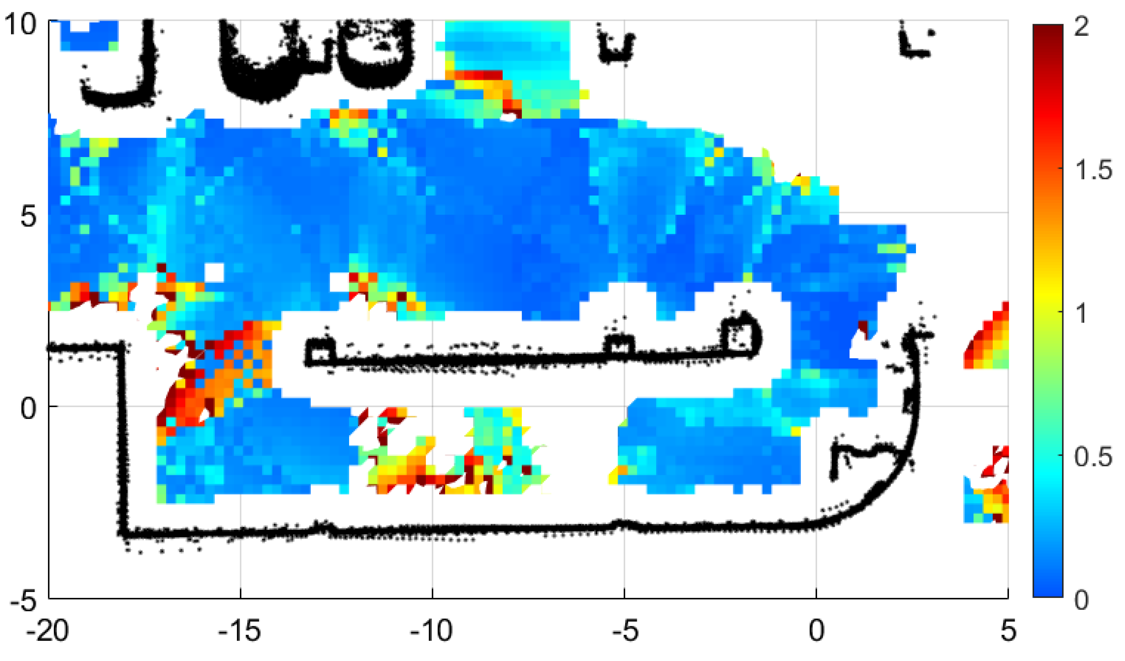
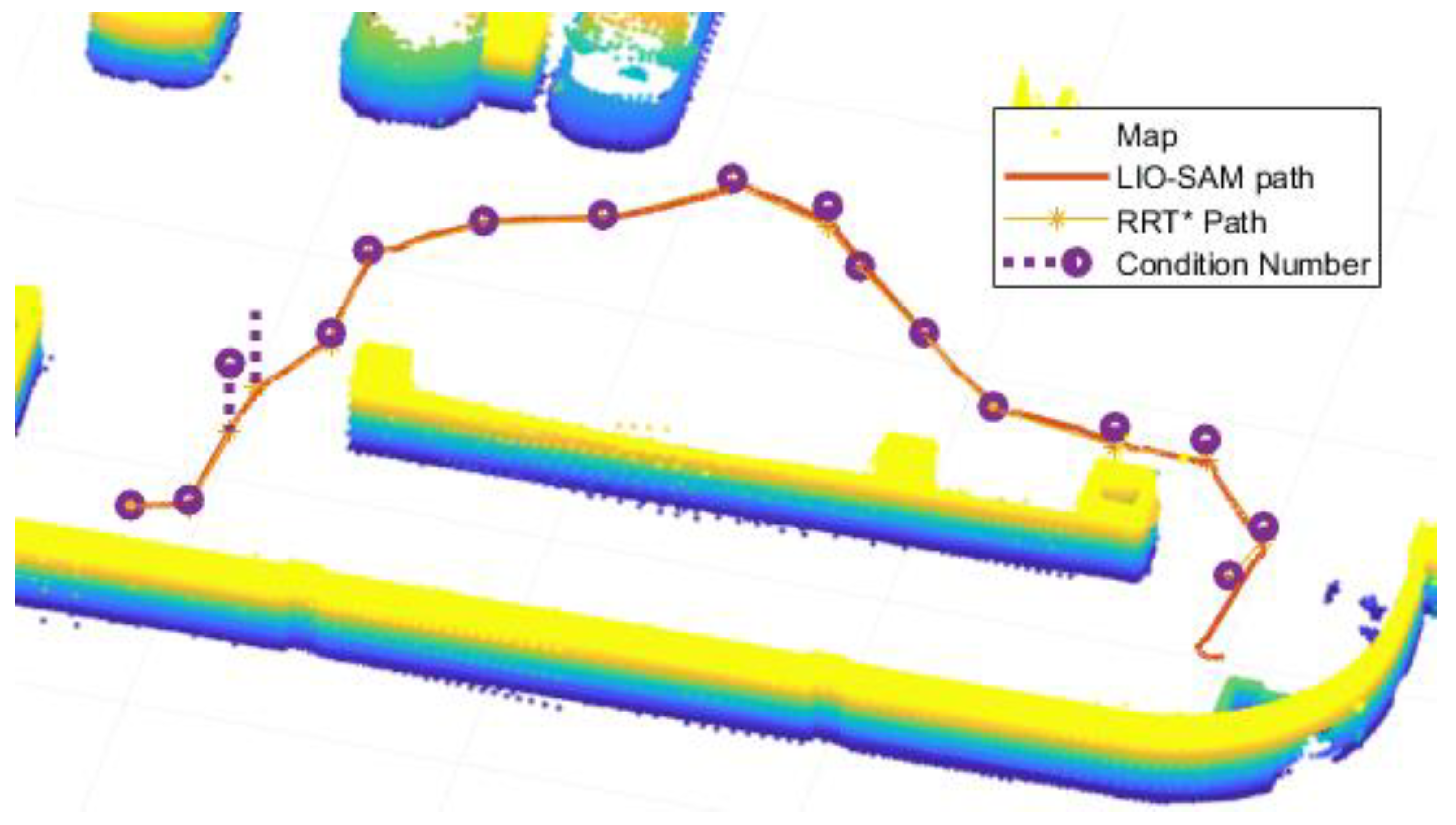
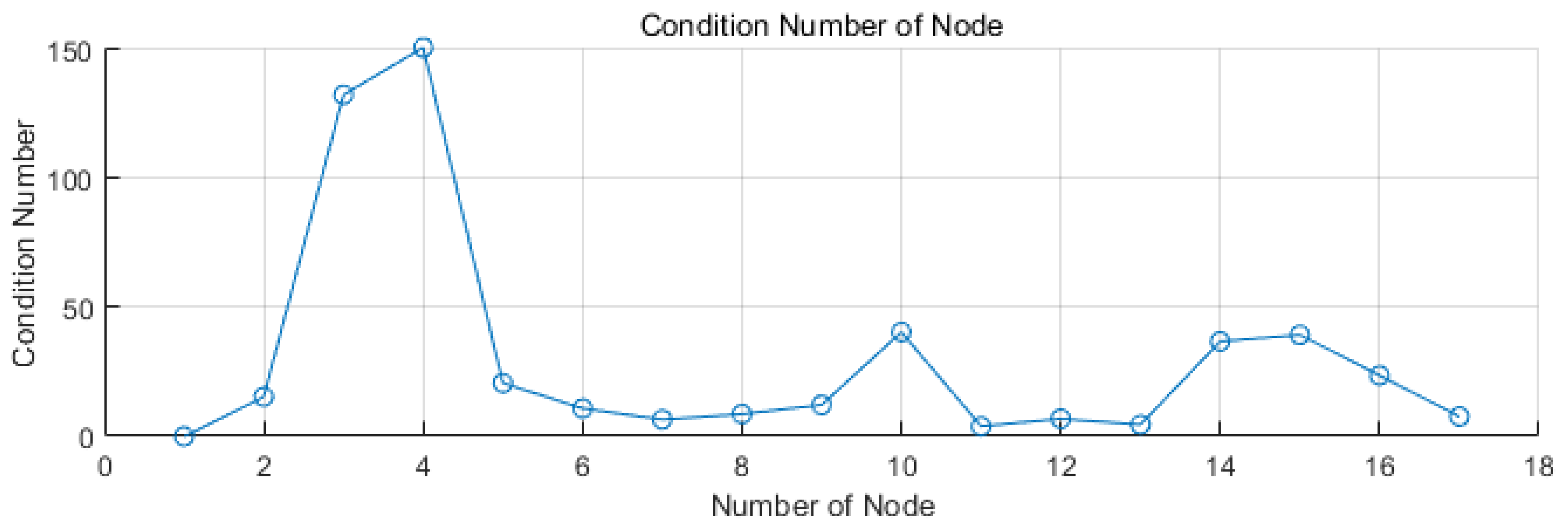
  • Observability: This function calculates observability and Condition Number  N c o n d . The wall detection method finds walls close to the node location  z n e w . It also serves as obstacle avoidance by returning 0 if the wall or obstacle is too close. Orthogonal vectors are extracted from the searched walls. The observability and Condition Number  N c o n d  are calculated using the extracted orthogonal vector and the location of the vector.
  • Near: A function that finds nodes within a certain radius centered on  z n e w .
  • ChooseParent: Finds and returns the node  z m i n  that makes the cost of  z n e w  the smallest among  Z n e a r .
  • InsertNode: A node connected to  z m i n  as a parent and  z n e w  as a child applies the tree τ.
  • Rewire: When  z n e w  is set as a parent among  Z n e a r , nodes with a smaller cost are found and changed.

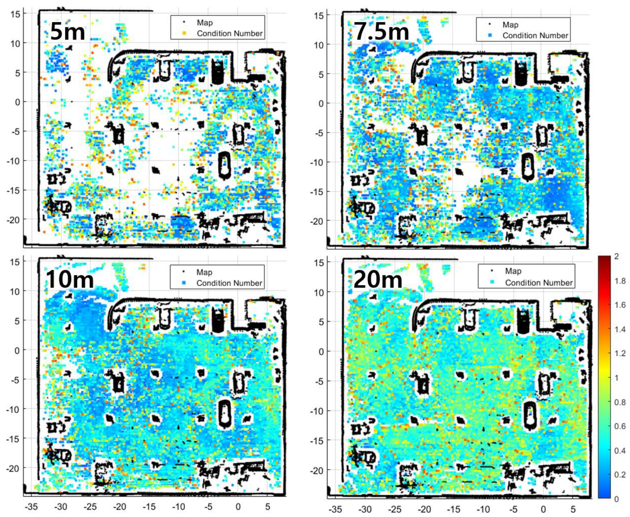
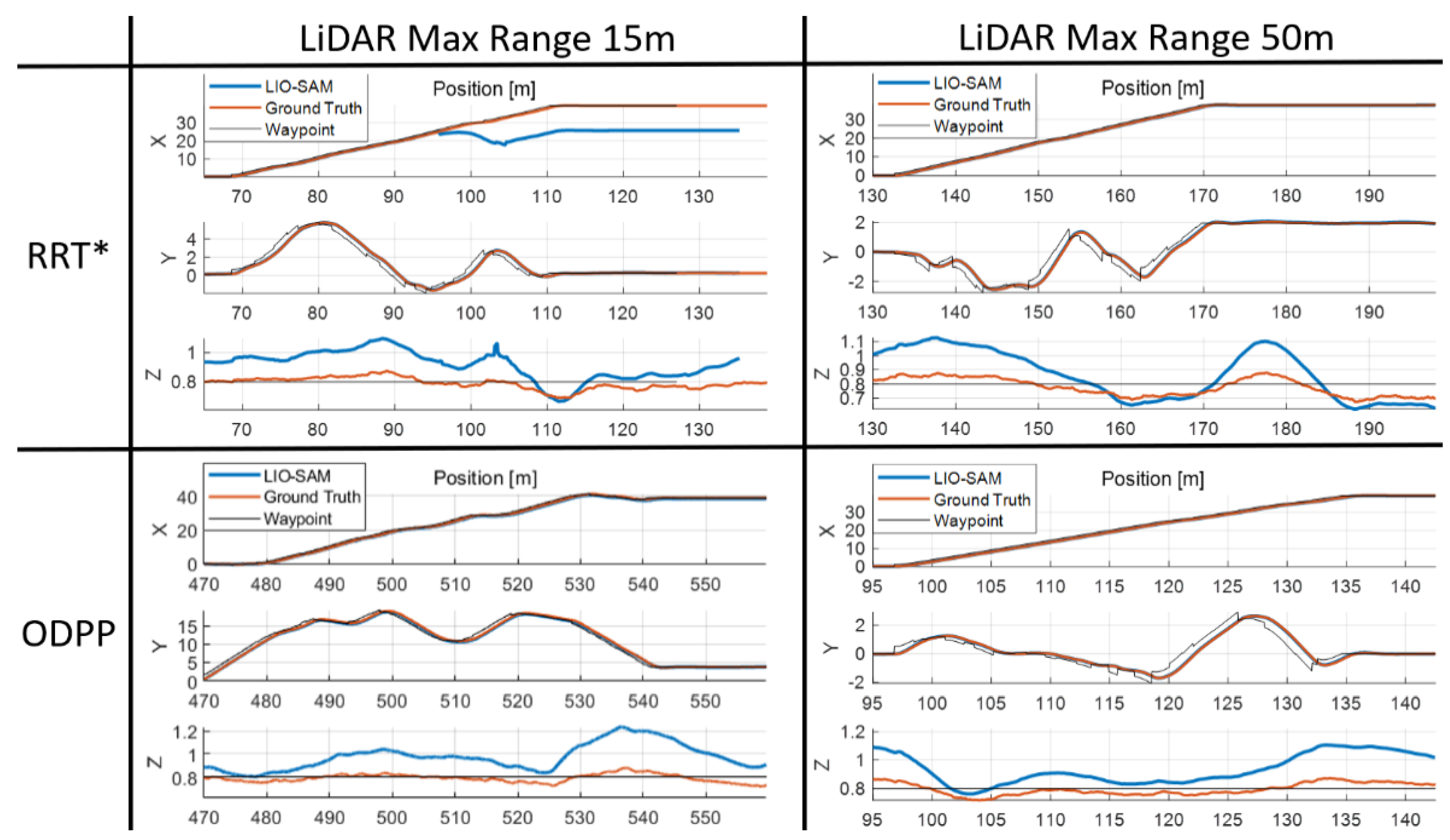
4.2. Simulation and Experimental Result

A simulation study was first performed to verify the observability-driven path planning algorithm. The simulation environment is the same as in the maze of Figure 7. The start and end points of the route are arbitrarily placed at both ends of the open area, and the maximum detection range of LiDAR is set to 15 m. It is evident that the shortest path is to pass through the lower corridor without any obstacles on it.
Figure 9 shows the tree of the constructed path based on the observability-driven path planning algorithm in Algorithm 1. As observed in the figure, no nodes are created through the lower corridor despite its distance advantage. Additionally, the upper corridor has discontinuity of the tree. This is due to the degraded condition number through the passage in the third room, where it is noted that the LiDAR measurements cannot satisfy the required rank of the observability matrix in the middle of passage. On the other hand, the path located in the middle corridor provides an optimal path without loss of observability quality for a given lidar measurement distance and FOV coverage. Through this, it is possible to avoid a path in which the SLAM navigation solution is degraded because observability is not guaranteed regardless of path length. Consequently, this results in a successful mission in an exploration area where error correction such as loop closure is not available.
For performance evaluation, the proposed ODPP was compared with the conventional path planning method, i.e., RRT*. The following Figure 10 shows the localization performance of LiDAR SLAM (i.e., LIO-SAM) with different sensor ranges and planning methods. In the upper left subplot, it can be observed that localization error increases to greater than 10 m in the x-axis due to the degraded observability. In contrast, the localization error is maintained within the sub-meter level due to good observability condition. Furthermore, it can be noted that if the LiDAR range is extensively enlarged, then the localization error becomes negligible between the conventional RRT* and the proposed ODPP scheme (as illustrated in the right subplots in the following Figure 10).
To test the proposed algorithm experimentally, an indoor autopilot test using the sensor platform onboard an autonomous vehicle was conducted. The motion of the vehicle is precisely manipulated by four-wheel motor control through the onboard microcomputer board, STMicroelectronic’s ARM Cortex-M4. Intel’s NUC11PAHi7 was used as the computing and mission planning platform and the OS is Ubuntu 18.04; ROS uses melodic.
The onboard sensor module contains LiDAR and IMU. In detail, LiDAR is Ouster’s OS0-32 (horizontal field of view is 360°, Vertical FoV is ±45°, Max range: 50 m) and IMU is Vectornav’s VN-100. Figure 11 shows the detailed block diagram of the hardware configuration.
To observe the path decision characteristics depending on navigation quality, the test environment was designed such that it was difficult to guarantee the SLAM performance. As shown in Figure 12b, a straight wall space without any obstacle was employed, which is similar to the lower corridor in Figure 9.
To check the observability quality distribution, the condition number map was first drawn. Figure 13 shows the condition number map over the experimental environment. Due to the constraints of the experimental environment, we calculated observability and the condition number by limiting the LiDAR maximum range to a radius of 6 m, while condition number maps were formed at 0.1 m intervals. Specifically, in Figure 13, it is observed that the condition number is high in the middle region of the lower lane; i.e., a straight path without obstacles. In the middle of the path, the condition number itself is unavailable as the rank condition is not met. As a result, the distributed score map can be effectively used for candidate node generation during the path planning process in a real experiment. In Figure 13, a color bar indicating condition number (1/100) graphically illustrates the candidate region of navigation performance.
Figure 14 shows the autopilot experimental result using the sensor measurement onboard the vehicle. Here, the experimental conditions were the same as in Figure 13 with a LiDAR maximum range of 6 m. Observing the tree of RRT* in the figure, the vehicle chooses to pass through the upper passage and reaches the destination point. In view of the location of the departure and arrival points, the shortest path is through the obstacle-free way. However, in this case, full rank condition cannot be achieved due to horizontal measurement deficiency. Thus, the suggested observability-driven path planning algorithm allocates a high-risk tree in this region, and accordingly the node cannot be created. Therefore, a route is created on the upper path where pillars or cars are recognized.
Given the final path as shown in Figure 15, the condition number was calculated to be less than 150. When analyzed through the condition number map, it was confirmed that the performance of SLAM was good at values below 200. Therefore, there is little possibility of divergence of SLAM due to matching failure during route driving. When the vehicle traveled along this route, it arrived at the destination without distortion of the map or divergence of location.

5. Results and Discussion

This study addresses the problems caused by map distortion or location estimation failure while driving with LiDAR SLAM. The goal was to identify topographically unfavorable locations for SLAM using observability analysis. When analyzing the observability rank in the 3D point cloud map, there were cases in which the SLAM diverged even with the full rank. The results of this paper were obtained by applying the condition number to these cases. This result was applied to the route planning algorithm to confirm that the vehicle reached the destination without divergence in navigation.
The observability analysis in this paper can be applied to Vision SLAM. Vision SLAM has a higher probability of map distortion compared with 3D LiDAR. The reason for this is that the FoV is relatively narrow. Therefore, it could be extended to a study determining which direction the camera should look from a specific location. In the future, this study will expand the path planning algorithm to an unknown environment exploration algorithm. Through this, we plan to research autonomous mapping without map distortion.

Author Contributions

Conceptualization, D.K.; methodology, B.L.; software, D.K.; validation, D.K. and S.S.; formal analysis, D.K.; investigation, D.K.; resources, B.L.; data curation, D.K.; writing—original draft preparation, D.K.; writing—review and editing, S.S.; visualization, D.K.; supervision, S.S.; project administration, S.S.; funding acquisition, S.S. All authors have read and agreed to the published version of the manuscript.

Funding

This research was funded by the Korean National Research Fund (NRF-2022R1A2C1005237), the Unmanned Vehicles Core Technology Research and Development Program through the National Research Foundation of Korea (NRF-2020M3C1C1A01086408) and a Korea Research Institute for defense Technology planning and advancement (KRIT) grant funded by the Korea government (DAPA (Defense Acquisition Program Administration)) (KRIT-CT-22-030, 2023).

Data Availability Statement

Not applicable.

Conflicts of Interest

The authors declare no conflict of interest.

References

  1. Shan, T.; Englot, B.; Ratti, C.; Rus, D. LVI-SAM: Tightly-Coupled Lidar-Visual-Inertial Odometry via Smoothing and Mapping. In Proceedings of the 2021 IEEE International Conference on Robotics and Automation (ICRA), Xi’an, China, 30 May–5 June 2021; pp. 5692–5698. [Google Scholar] [CrossRef]
  2. Zheng, C.; Zhu, Q.; Xu, W.; Liu, X.; Guo, Q.; Zhang, F. FAST-LIVO: Fast and Tightly-Coupled Sparse-Direct LiDAR-Inertial-Visual Odometry. In Proceedings of the 2022 IEEE/RSJ International Conference on Intelligent Robots and Systems (IROS), Kyoto, Japan, 23–27 October 2022; pp. 4003–4009. [Google Scholar] [CrossRef]
  3. Qin, T.; Li, P.; Shen, S. VINS-Mono: A Robust and Versatile Monocular Visual-Inertial State Estimator. IEEE Trans. Robot. 2018, 34, 1004–1020. [Google Scholar] [CrossRef]
  4. Shan, T.; Englot, B.; Meyers, D.; Wang, W.; Ratti, C.; Rus, D. LIO-SAM: Tightly-Coupled Lidar Inertial Odometry via Smoothing and Mapping. In Proceedings of the IEEE International Conference on Intelligent Robots and Systems, Las Vegas, NV, USA, 25–29 October 2020; pp. 5135–5142. [Google Scholar] [CrossRef]
  5. Xu, W.; Cai, Y.; He, D.; Lin, J.; Zhang, F. FAST-LIO2: Fast Direct LiDAR-Inertial Odometry. IEEE Trans. Robot. 2022, 38, 2053–2073. [Google Scholar] [CrossRef]
  6. Forster, C.; Pizzoli, M.; Scaramuzza, D. SVO: Fast Semi-Direct Monocular Visual Odometry. In Proceedings of the 2014 IEEE International Conference on Robotics and Automation (ICRA), Hong Kong, China, 31 May–7 June 2014; pp. 15–22. [Google Scholar] [CrossRef]
  7. Carrillo, H.; Reid, I.; Castellanos, J.A. On the Comparison of Uncertainty Criteria for Active SLAM. In Proceedings of the 2012 IEEE International Conference on Robotics and Automation, Saint Paul, MN, USA, 14–18 May 2012; pp. 2080–2087. [Google Scholar] [CrossRef]
  8. Maurovic, I.; Seder, M.; Lenac, K.; Petrovic, I. Path Planning for Active SLAM Based on the D* Algorithm with Negative Edge Weights. IEEE Trans. Syst. Man Cybern. Syst. 2018, 48, 1321–1331. [Google Scholar] [CrossRef]
  9. Palomeras, N.; Carreras, M.; Andrade-Cetto, J. Active SLAM for Autonomous Underwater Exploration. Remote Sens. 2019, 11, 2827. [Google Scholar] [CrossRef]
  10. Lim, H.; Jeon, J.; Myung, H. UV-SLAM: Unconstrained Line-Based SLAM Using Vanishing Points for Structural Mapping. IEEE Robot. Autom. Lett. 2022, 7, 1518–1525. [Google Scholar] [CrossRef]
  11. Jung, K.Y.; Kim, Y.E.; Lim, H.J.; Myung, H. ALVIO: Adaptive Line and Point Feature-Based Visual Inertial Odometry for Robust Localization in Indoor Environments. In Lecture Notes in Mechanical Engineering; Springer: Berlin/Heidelberg, Germany, 2021; pp. 171–184. [Google Scholar] [CrossRef]
  12. Zhang, C. PL-GM:RGB-D SLAM with a Novel 2D and 3D Geometric Constraint Model of Point and Line Features. IEEE Access 2021, 9, 9958–9971. [Google Scholar] [CrossRef]
  13. Bavle, H.; De La Puente, P.; How, J.P.; Campoy, P. VPS-SLAM: Visual Planar Semantic SLAM for Aerial Robotic Systems. IEEE Access 2020, 8, 60704–60718. [Google Scholar] [CrossRef]
  14. Qiu, Z.; Lin, D.; Jin, R.; Lv, J.; Zheng, Z. A Global ArUco-Based Lidar Navigation System for UAV Navigation in GNSS-Denied Environments. Aerospace 2022, 9, 456. [Google Scholar] [CrossRef]
  15. Yang, Y.; Huang, G. Observability Analysis of Aided INS with Heterogeneous Features of Points, Lines, and Planes. IEEE Trans. Robot. 2019, 35, 1399–1418. [Google Scholar] [CrossRef]
  16. Einhorn, E.; Gross, H.M. Generic NDT Mapping in Dynamic Environments and Its Application for Lifelong SLAM. Rob. Auton. Syst. 2015, 69, 28–39. [Google Scholar] [CrossRef]
  17. Mendes, E.; Koch, P.; Lacroix, S. ICP-Based Pose-Graph SLAM. In Proceedings of the SSRR 2016—International Symposium on Safety, Security and Rescue Robotics, Lausanne, Switzerland, 23–27 October 2016; pp. 195–200. [Google Scholar] [CrossRef]
  18. Lee, B.; Kim, D.G.; Lee, J.; Sung, S. Analysis on Observability and Performance of INS-Range Integrated Navigation System Under Urban Flight Environment. J. Electr. Eng. Technol. 2020, 15, 2331–2343. [Google Scholar] [CrossRef]
  19. Mirzaei, F.M.; Roumeliotis, S.I. A Kalman Filter-Based Algorithm for IMU-Camera Calibration: Observability Analysis and Performance Evaluation. IEEE Trans. Robot. 2008, 24, 1143–1156. [Google Scholar] [CrossRef]
  20. Gao, S.; Wei, W.; Zhong, Y.; Feng, Z. Rapid Alignment Method Based on Local Observability Analysis for Strapdown Inertial Navigation System. Acta Astronaut. 2014, 94, 790–798. [Google Scholar] [CrossRef]
  21. Yeon, S.; Doh, N.L. Observability Analysis of 2D Geometric Features Using the Condition Number for SLAM Applications. In Proceedings of the International Conference on Control, Automation and Systems, Gwangju, Republic of Korea, 20–23 October 2013; pp. 1540–1543. [Google Scholar] [CrossRef]
  22. Bavle, H.; Sanchez-Lopez, J.L.; de la Puente, P.; Rodriguez-Ramos, A.; Sampedro, C.; Campoy, P. Fast and Robust Flight Altitude Estimation of Multirotor UAVs in Dynamic Unstructured Environments Using 3D Point Cloud Sensors. Aerospace 2018, 5, 94. [Google Scholar] [CrossRef]
  23. Chen, S.; Zhou, W.; Yang, A.S.; Chen, H.; Li, B.; Wen, C.Y. An End-to-End UAV Simulation Platform for Visual SLAM and Navigation. Aerospace 2022, 9, 48. [Google Scholar] [CrossRef]
  24. Karaman, S.; Frazzoli, E. Sampling-Based Algorithms for Optimal Motion Planning. Int. J. Robot. Res. 2011, 30, 846–894. [Google Scholar] [CrossRef]
Figure 1. Geometric relationship between a specific position  P  and surrounding walls.
Aerospace 10 00492 g001
Figure 2. Velocity and attitude prediction controller structure.
Aerospace 10 00492 g002
Figure 3. Point clouds generation via topological detection scheme.
Aerospace 10 00492 g003
Figure 4. Condition number map in an environment with surrounding walls.
Aerospace 10 00492 g004
Figure 5. Condition number map in an environment where the left side is open and three sides are closed.
Aerospace 10 00492 g005
Figure 6. Condition number map in an environment where the upper and lower surfaces are open.
Aerospace 10 00492 g006
Figure 7. (a) Maze environment in Gazebo simulator. (b) Condition number map of maze environment.
Aerospace 10 00492 g007
Figure 8. Condition number map for each LiDAR maximum distance in an underground parking lot.
Aerospace 10 00492 g008
Figure 9. Tree of path planning algorithm in the maze environment. The blue dot is the starting point, the magenta dot is the destination, and the black dot is the point cloud map. The line represents the ODPP tree, and the color varies according to the condition number. Higher values are shown in red, and lower values are in yellow.
Aerospace 10 00492 g009
Figure 10. RRT* vs. ODPP Algorithm by LiDAR Max Range.
Aerospace 10 00492 g010
Figure 11. Test platform schematic diagram. Green dotted line: mission computer composed of NUC. Blue dotted line: vehicle controller based on Cortex-M4. Black dotted line: actuator hardware.
Aerospace 10 00492 g011
Figure 12. Experimental environment; (a) complicated obstacles; and (b) straight corridor.
Aerospace 10 00492 g012
Figure 13. Condition number map in experimental environment.
Aerospace 10 00492 g013
Figure 14. Tree of path planning algorithm in the experimental environment.
Aerospace 10 00492 g014
Figure 15. The condition number of the path finally selected in path planning.
Aerospace 10 00492 g015
Disclaimer/Publisher’s Note: The statements, opinions and data contained in all publications are solely those of the individual author(s) and contributor(s) and not of MDPI and/or the editor(s). MDPI and/or the editor(s) disclaim responsibility for any injury to people or property resulting from any ideas, methods, instructions or products referred to in the content.

