1. Introduction
Deviations of the compressor geometries of design values can occur during the manufacturing process of an aeroengine, resulting in a significant impact on aerodynamic performance, being mainly characterized by a mean-shift, in addition to increased variance [
1]. As tools to quantify the effect of geometric deviation on performance uncertainty, as well as for pinpointing the most sensitive source, uncertainty quantification (UQ) and sensitivity analysis (SA) have drawn increased attention in recent years [
2,
3,
4,
5,
6]. Moreover, a robust design has been progressively implemented in the field of aerodynamic design for turbomachinery, striving to sustain aerodynamic performance in a multidisturbance environment [
7,
8,
9]. To determine the aerodynamic performance uncertainty, a collection of blade profiles with variations is required. Therefore, the model of deviations needs to be explicitly specified. After determining the deviation model, various mathematical tools and analytical techniques can be applied to the blades with deviations, so as to obtain an accurate evaluation of their aerodynamic performance. The accuracy of the deviation model has a direct and demonstrable impact on the results of the entire procedure for solving the uncertainty problem.
Currently, two categories of deviation modeling techniques exist: geometry-based and performance-based. The first category has four primary deviation modeling techniques:
The isolated deviation model superimposing method. This method introduces deviations at isolated positions on the blade, assuming that no deviations exist at other positions. Kumar [
10] superimposed the Hicks–Henne bump on the blade surface to study the performance changes of blade profiles after erosion. Goodhand et al. [
11] placed the Hicks–Henne bump on the blade surface to analyze the impact of deviations on the incidence range;
The designed geometric parameter disturbing method. This method has been investigated extensively [
12,
13,
14,
15]; Lange et al. [
12] utilized an optical measurement technique to obtain the coordinate points of the blade surface. Then, they used a blade to parameter (B2P) software to identify 18 design parameters of the blade profiles in each section. They found that a mean section could describe, with deviations, the most important changes in blade geometry. Furthermore, they investigated the covariance matrix of the design parameters. In addition, they utilized Monte Carlo sampling, in conjunction with a covariance constraint, to replicate the real deviations as closely as possible. Notably, the B2P software played an essential role in the process of disturbing design parameters. Identifying the camber line is crucial in the B2P process, particularly near the leading edge (LE) and the trailing edge (TE). Under the influence of high curvature, geometric parameters around the edges are insufficiently accurate to be determined;
The Eigenmode-based dimension reduction analysis method. The most widely used methods for UQ or SA studies are principal component analysis (PCA) and Karhunen–Loeve expansion methods. The PCA approach can be understood as the extraction of modes with significant shape deviation scatters. This method was introduced by Garzon [
1], for the modeling of deviations in turbomachinery, and has since been utilized in numerous investigations of uncertainty [
16,
17,
18,
19,
20]. The benefit of this technique was that the covariance relationship between the deviation points could be maintained with a small number of variables. This covariance information could effectively reflect the inherent relationships among the deviation points on the blade surface during the specific manufacturing process; for example, nearby points on a blade surface tend to have similar deviations;
The blade surface control points disturbing method. In this method, the positions of discrete surface points are modified to obtain a new blade profile. Kumar [
10] modeled the blade profile using the Hicks–Henne function, before then disturbing each control point to generate new blade profiles. Wong et al. [
21] produced a new blade profile by vertically perturbing 20 control points on the blade surface and then connecting the points using spline curves.
Owing to the complicated nonlinearly coupled impact between multiple variations on the blade, accurately capturing the real changes in aerodynamic performance is difficult for those geometry-based models which are characterized by only a small number of parameters [
5,
22].
The performance-based models relied on the gradient information of the target performance. The singular value decomposition (SVD) of the Jacobian matrices of the target performance [
23] (in addition to active subspace methods [
21]) were employed, so as to produce reduced–order models of deviations. Dow and Wang [
23] created a nested model based on the gradient information of two performance quantities of interest: first, the PCA technique was utilized to determine the modes of blade deviations; and second, the SVD method and the Jacobian covariance matrix were utilized, so as to determine which mode combinations had a major impact on performance. Constantine et al. [
24] presented the active subspace method, which was applicable to multiobjective functions [
25]. The active subspace approach determined the major direction of the global performance gradient and identified the combination of design parameters that had the greatest impact on performance across the entire design space. Wong et al. [
21] applied the active subspace method to determine whether the performance of a newly manufactured blade was up to standard. Without the adjoint technique, acquiring gradient information on the target performance would be a cumbersome task [
23]. The drawback of performance-based models is that the final form of deviations cannot normally capture the covariance relationship between coordinate points on the blade surface, which is essential for accurately reflecting the manufacturing process.
The model of deviations has a direct impact on the evaluation of statistical performance in the compressors. Manufacture deviations could cause the performance mean shift and performance variance [
26]. However, there is still a lack of quantitative evaluation regarding the accuracy of these two parameters when utilizing geometry-based and performance-based modeling methods.
This study focuses on the impact of deviation models on the statistical evaluation of the aerodynamic performance in compressors. Herein, the sensitivity-correlated principal component analysis (SCPCA) method, which is both geometry-based and performance-based, has been proposed for the first time to model deviations in compressors. By introducing weighting factors, the SCPCA method could identify modes with smaller eigenvalues in the PCA method, but with a significant impact on the airfoil performance. The weighting factor played a role in reflecting the influence of deviation modes on aerodynamic performance. To verify the feasibility of the SCPCA method, section profiles of rotor blades from a high-pressure compressor stage were analyzed using this method. The interval estimation method was used to quantitatively evaluate the errors of UQ analysis based on the PCA and SCPCA methods. Moreover, the working mechanism of the SCPCA method with higher accuracy on UQ analysis was investigated. The results indicated that the deviation modeling approach utilized in the SCPCA method was particularly effective at regions with sensitive flow phenomena, as it can significantly increase the accuracy of evaluating performance variability. Therefore, the proposed SCPCA method showed good potential for deviation modeling in the field of UQ, SA, and robust design.
3. SCPCA Method
The relationship between the geometry and the aerodynamic performance of a compressor blade is complex and nonlinear. Large deviations in geometry may have a slight effect on aerodynamic performance. This nonlinear relationship results in a limitation in the implementation of the PCA approach, as this method only detects the principal modes of deviations based on the geometric scale. However, some small-scale deviations that have a major impact on performance are totally ignored during the modeling procedure. Therefore, in the process of modeling deviation, establishing the correct covariance relationship is crucial to accurately reflect the actual manufacturing process, with particular attention given to small-scale deviation, which has a substantial impact on aerodynamic performance. This problem can be easily resolved in the SCPCA method by introducing the weighting factors of the eigenmodes.
As discussed in the previous section, on the application of PCA method, the , which refer to the set of principal modes for the deviation modeling, could be formed using the first four modes with the largest eigenvalues. To denote the complementary set of with respect to all modes obtained using the PCA method, we have used the symbol . In the SCPCA method, the modes that are included in the set of but have a significant impact on the aerodynamic performance have been identified and utilized for deviation modeling. Assuming the subspace spanned using the eigenvectors in contained a special unit vector , the deviation mode represented by the vector had a significant impact on the blade performance, and eigenmodes in the set of with smaller angles between them and had a greater impact on the performance. Therefore, the importance of the eigenvectors in can be ranked by the angle between each eigenvector and , in addition to the scatter of the deviation data along each eigenvector. After obtaining the mode ranking of the impact on the blade performance, the eigenvectors in that had a greater impact on the aerodynamic performance could be selected to form a new set of . In the SCPCA method, the union of and has been used for the final deviation modeling.
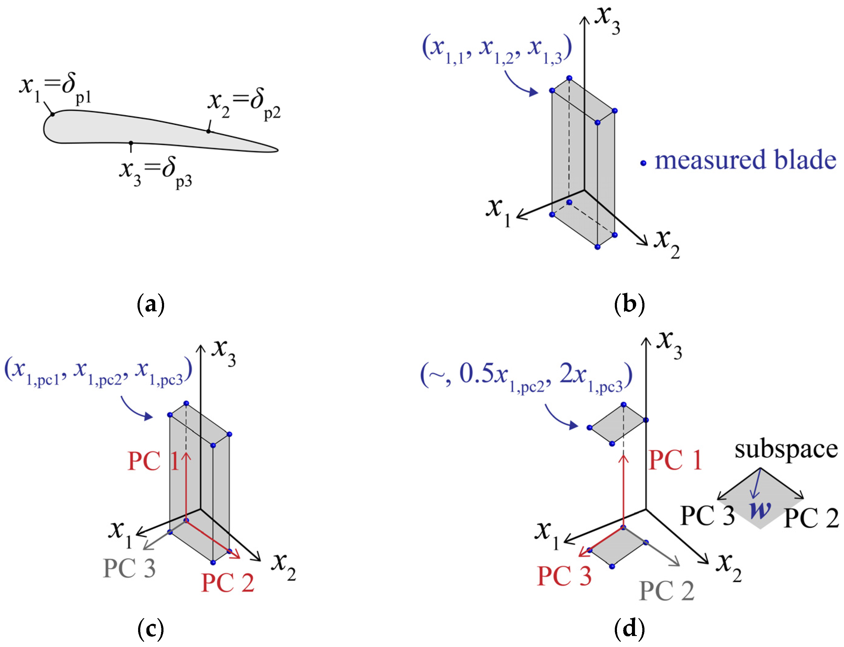
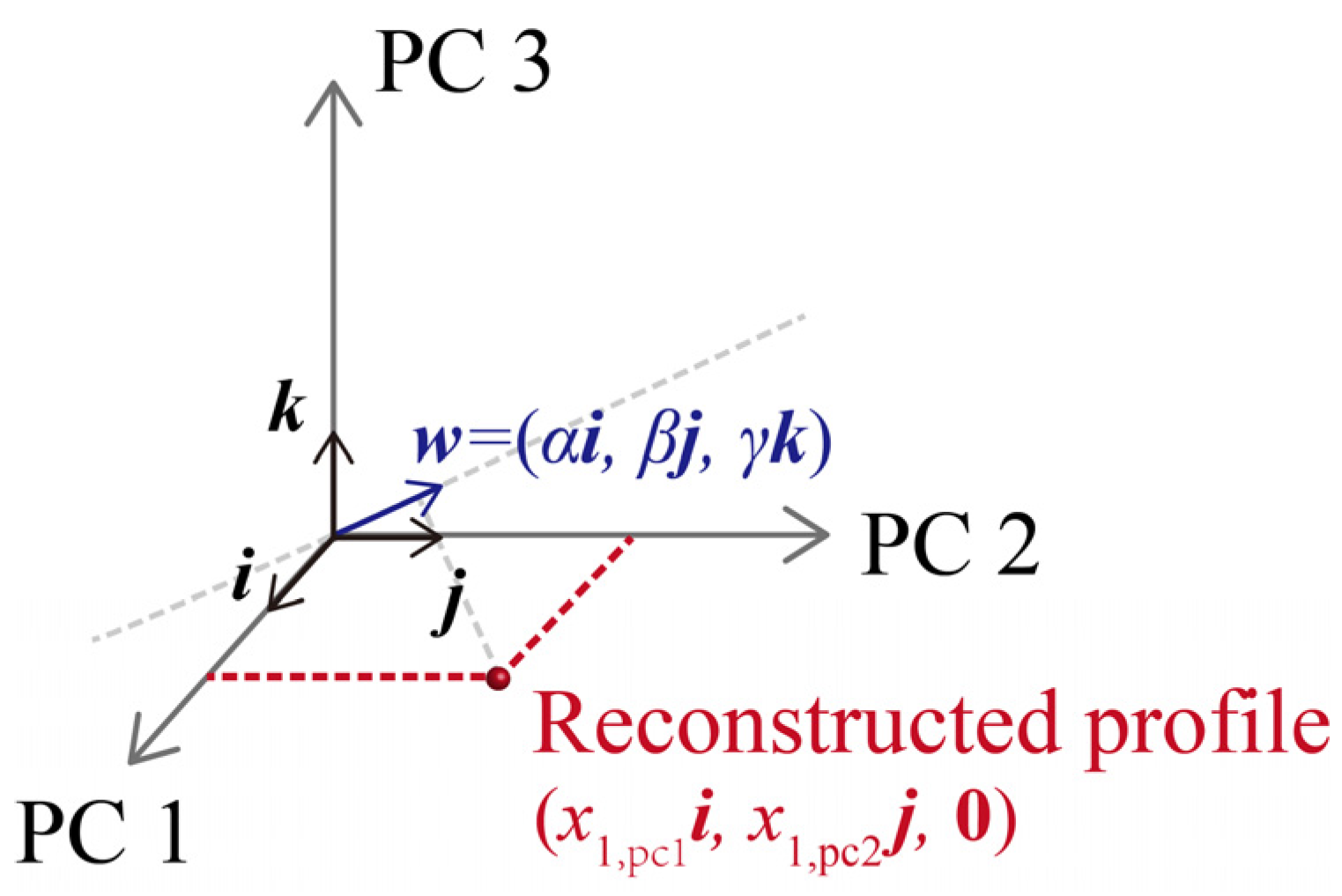
Figure 4 illustrates the process of the mode selection in the SCPCA method. Assuming that there are three positions (p1, p2, and p3) shown in
Figure 4a for measuring blade deviations, the normal deviations
for each measured blade at these three positions were represented as
-coordinate values. Then, each measured blade could be represented as a three-dimensional coordinate point
depicted in
Figure 4b. Assuming that a total of eight real blades have been measured, so, the eight blue dots can be drawn in
Figure 4b. In this context, the problem of deviation modeling concerns how to use a smaller number of variables so as to describe the original 3-dimensional deviation data.
Figure 4c shows the deviation modes identified using the PCA method. Since the projection of the original deviation data onto the first principal component (PC 1) and the second principal component (PC 2) had a large scatter, the PC 1 and PC 2 (marked in red in
Figure 4c) have been selected in the PCA method when choosing two modes for deviation modeling. In the orthogonal coordinate system composed of principal component eigenvectors, the coordinate
has been transformed into the coordinate
. The vector
, defined in the last paragraph, was located in the subspace spanned by PC 2 and PC 3, as shown in
Figure 4d. In this figure, the projection value of
onto PC 2 was assumed to be twice that onto PC 3. The projection values of
can reflect the magnitude of the angle between
and the eigenvectors. Then, using these projection values as weighting factors of PC 2 and PC 3, the original measured data can be scaled along each eigenvector. Based on the variance of the scaled data, the eigenvector with the greater impact on the performance could be determined.
Appendix A provides a detailed explanation of the rationale behind using projection values for data scaling and sorting the scaled data according to variance. In
Figure 4d, PC 3 was the eigenvector that had the greatest impact on the performance, rather than PC 2, despite PC 2 being ranked higher in the PCA method. Therefore, when selecting two modes for deviation modeling, the PC 1 and PC 3 (marked in red in
Figure 4d) have been selected in SCPCA method.
In the SCPCA method, the weighting factor of each eigenmode
was determined using the projection value of the unit vector
onto the eigenvector.
From the perspective of signal similarity,
also reflected the degree of similarity between the sensitive mode represented by
and various eigenmodes
. After obtaining the weight corresponding to each mode, the weight matrix
could be determined. The projection value of the scaled measurement data onto each eigenmode can be calculated using the following formula:
where
,
represents the projection values of all scaled data on the
-th eigenmode. By sorting the variance of the
in descending order, those eigenmodes in
that had a greater impact on the blade performance could be determined. Thus, the subset
of
can be obtained using the SCPCA method. Furthermore, the union of sets
and
contained all the modes employed by the SCPCA method for deviation modeling:
where
is the reduced-order model of the deviation obtained using the SCPCA method, and
is the total number of selected modes. Notably, all SCPCA eigenvectors were included in the PCA eigen vectors. The only difference between the two methods is that the SCPCA method selects several modes with small corresponding eigenvalues in the PCA method. These additional modes are viewed as having a significant impact on the blade aerodynamic performance. The eigenvectors in the SCPCA technique were derived from the eigenvectors in the PCA method, and the principal modes in the PCA method were also preserved. Hence, the covariance relationship between the deviation points can be maintained. The covariance relationship provided the SCPCA method with the same ability to reflect the actual manufacturing process as the PCA method. Additionally, the SCPCA method utilized some neglected aerodynamically sensitive modes to model deviations. Therefore, the SCPCA is also a performance-based method.
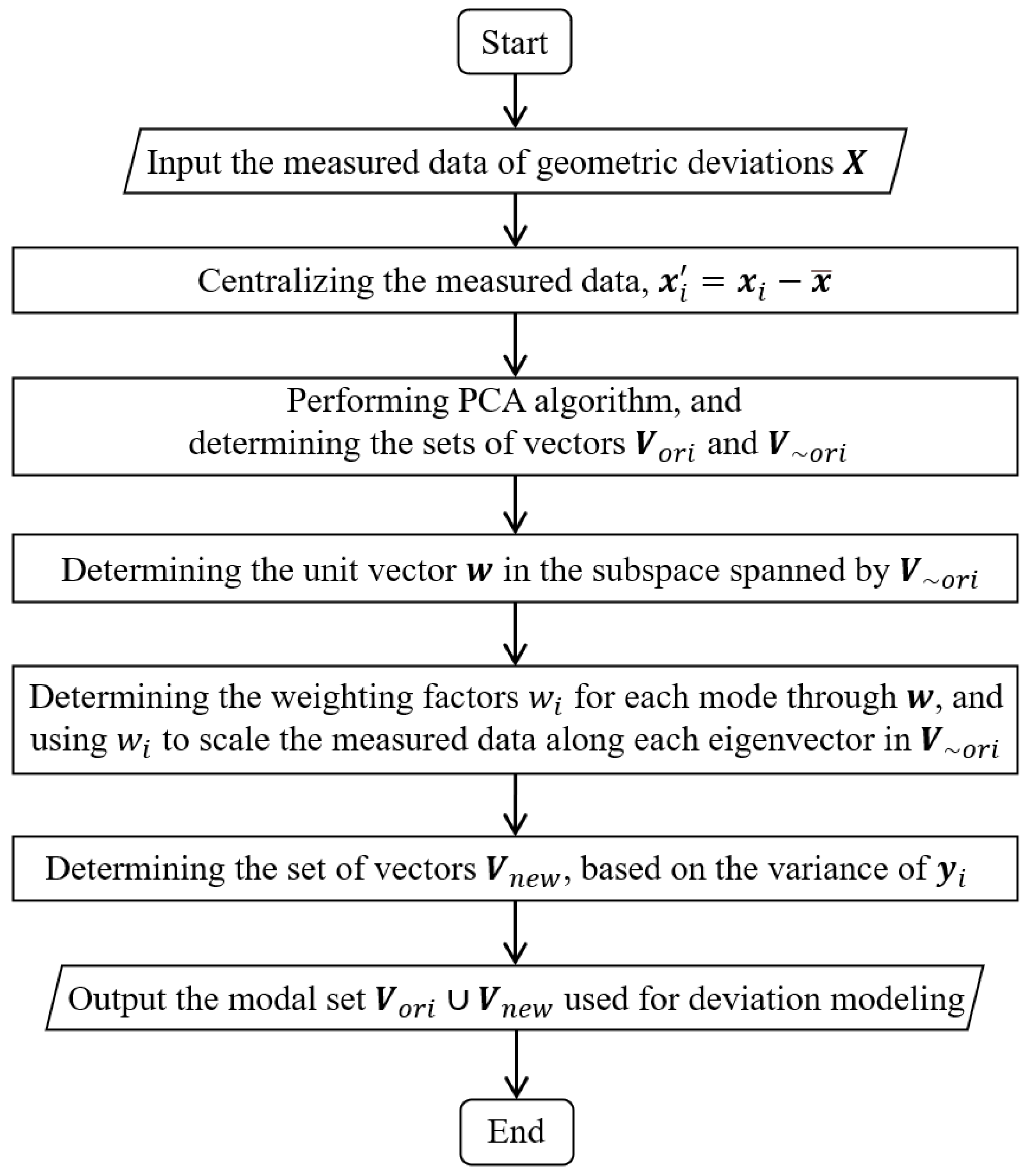
Figure 5 displays the algorithmic flowchart of the SCPCA method. The operational steps of the SCPCA method can be summarized as follows:
Centralize the measured data and apply the eigenvalue decomposition of the covariance matrix to determine the principal components of PCA corresponding to the manufacture deviations.
Sort the principal components in descending order based on their eigenvalues. The top-ranked modes which can reflect most of the geometric deviations constitute the set of . The complement of is named .
Determine the unit vector . The deviation mode represented by has a significant impact on the blade performance.
Determine the weighting factors for each mode and scale the original measured data along each eigenvector in with .
Sort the eigenmodes in in descending order based on the corresponding variance of the scaled data . The top-ranked eigenvectors in form the set of .
The union of the sets of and contains all the modes used for the deviation modeling in the SCPCA method.
The central idea of the SCPCA method is to retain the principal modes
obtained from the PCA method, and at the same time, rank the remaining modes based on the performance sensitivity information, and select the modes in
that have a greater impact on the blade performance. It is worth noting that one variation of the PCA method is the kernel PCA (KPCA) method [
33]. The differences between the SCPCA and KPCA methods need to be mentioned to avoid conceptual confusion. The KPCA method often requires a dimensionality increase in the original data, and the final basis obtained from the transformed data is often nonlinear when mapped to lower dimensions. In contrast to the KPCA method, the SCPCA method performs computations in the low-dimensional space spanned by
, and the modes finally selected using the SCPCA method are still within the modes determined with the PCA method. The purpose of sorting the modes within the framework of the PCA method is to ensure the orthogonality of all modes and the independence between random variables, which will give the deviation model a simple form.
4. Determination of Sensitivity-Based Weighting Factor for SCPCA
In the SCPCA method, the unit vector
was used as the basis for sorting the modes in the set of
set according to their impact on aerodynamic performance. Owing to the coupled effect between modes on the aerodynamic performance, determining how performance changes is challenging when superposing different modes on the blade surface. However, resolving the sensitivity of the aerodynamic performance is simple when there is a single deviation on the blade surface. This study recommends setting the sensitivity of the aerodynamic performance so as to determine the unit vector
and the weight factors
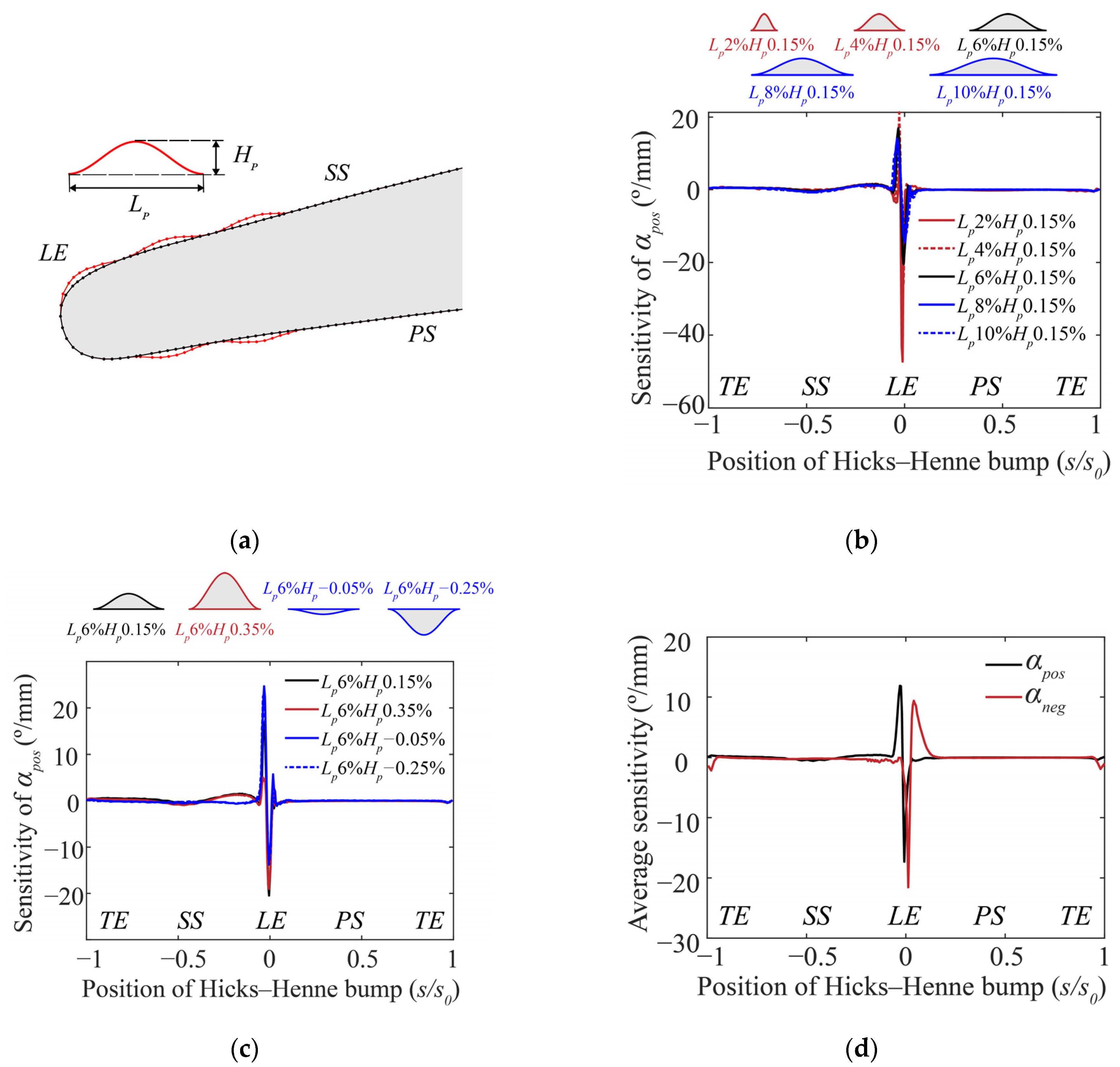
. The sensitivity along the blade surface was obtained based on the calculation of aerodynamic gradient with local geometry variation on blade surface. The deviation model of the Hicks–Henne bump shown in
Figure 6a was used to disturb the local geometry on the blade surface, as used by Goodhand [
31]. The mathematical formula of the Hicks–Henne bump is as follows:
where
is the normal deviation on the blade surface with respect to the nominal profile, and
and
denote the width and height of the deviation, respectively. The aerodynamic sensitivity
of the blade profile can be approximated using the first-order difference quotient:
The sensitivity values of the blade surface at each point constitute the vector
. By projecting the vector
onto the subspace spanned by
and normalizing the resulting projection vector, the unit vector
can be easily obtained. Once
has been determined, the weighting factors
corresponding to each eigenmode can be calculated using the method described in
Section 3.
Table 2 presents the parameters of Hicks–Henne bumps used to calculate the aerodynamic sensitivity. These selected parameter values of bumps are based on the deviation amplitude and the waviness of the blade surface extracting from the real manufactured blades. Along the blade surface, 185 locations that were denser at the LE and sparser elsewhere on the blade surface were defined. In each location, 20 geometry variations determined according to the combination of parameters listed in
Table 2 were applied individually to generate blade samples with geometry deviation. Finally, blade performances for all blade samples were calculated using MISES, and a total of 3700 samples were obtained to calculate the sensitivity of aerodynamic performance. Performing calculations for so many samples is intended to obtain as accurate a result for vector
as possible.
Figure 6b,c show the results of the SA of the positive incidence range
. Evidently, the positive incidence range is susceptible to the deviations around the LE and the front 20% arc length on the suction surface (SS). The deviations on the pressure surface (PS) and TE had a lesser significant effect on the positive incidence range. Additionally, the different shapes of the Hicks–Henne bump had a direct effect on the sensitivity value, which indicated the nonlinear effect of the performance sensitivity with geometry variation. However, this nonlinear sensitivity effect did not change the sensitivity distribution along the blade surface. To obtain a single weighting factor for each measured point in the SCPCA method, the 3700 sensitivity values were simply averaged to obtain the result shown in
Figure 6d. The mean sensitivity values of the positive incidence range and the negative incidence range at each measured point have been utilized as vector
to determine the weighting factors in the following sections.
Compared to the PCA method, the additional computational cost of the SCPCA method is mainly due to the calculation of the unit vector . The specific value of this additional cost depends on the method used to determine the vector . In this study, the vector was determined by placing Hicks–Henne bumps on the blade surface to obtain the sensitivity of aerodynamic performance. Consequently, when compared to the PCA method, an additional computation of aerodynamic performance was performed for 3700 blade profiles with local geometric variations, which took approximately 96 CPU core hours (Intel R Core TM i7 10700 CPU). If either an adjoint method or a global sensitivity analysis strategy are employed to determine the vector , there is potential to reduce this additional computational cost, which will be a focus of future work.
5. Comparison of the Performance of PCA and SCPCA Methods
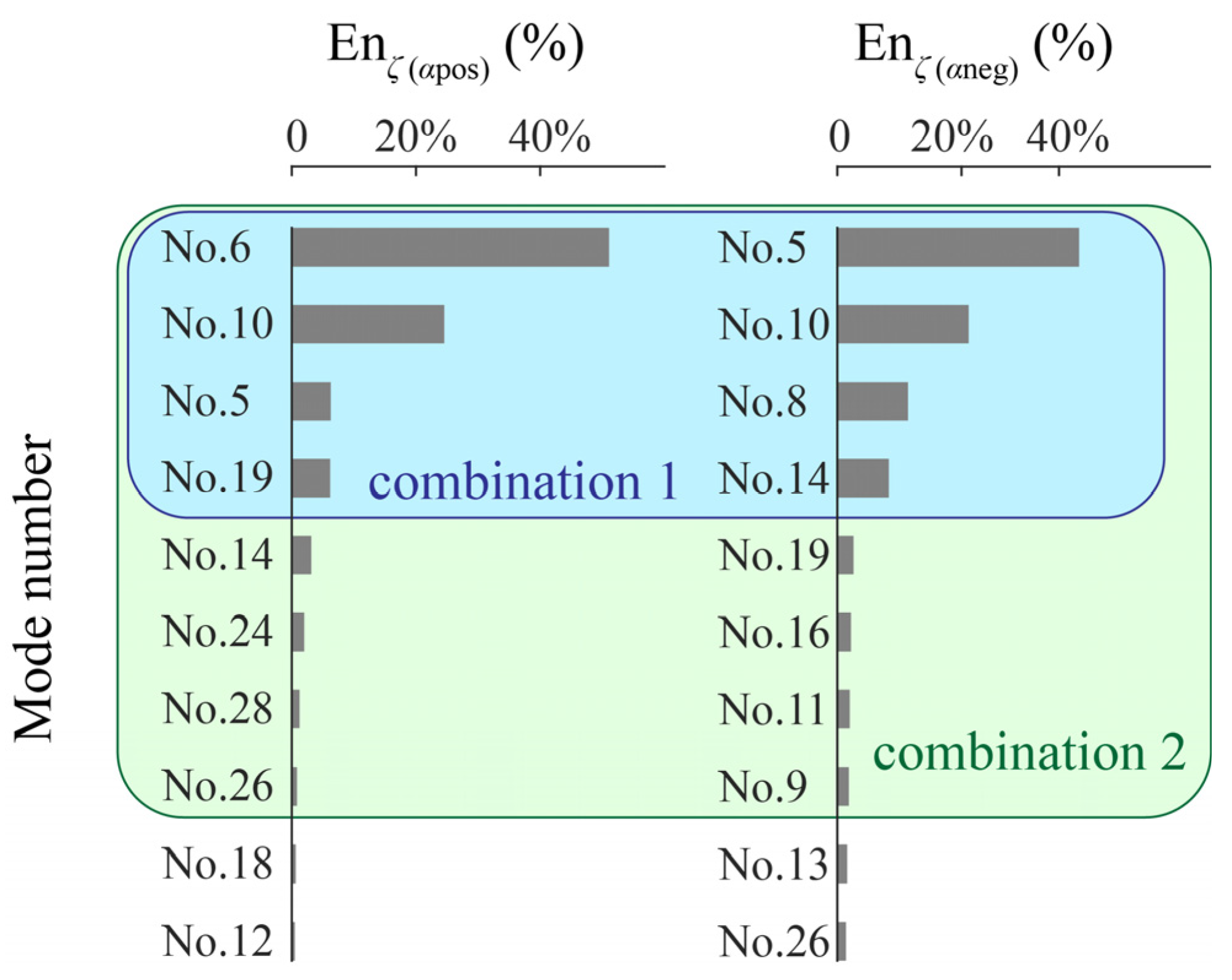
After determining the weighting factors using the mean sensitivity values of the positive incidence range and the negative incidence range, the ranking of the modes in
can be determined based on the variance of the scaled data.
Figure 7 shows the ordering of the eigenmodes corresponding to the sensitivity values of the positive incidence range and the negative incidence range, respectively. The definition of sensitivity-based energy ratio was as follows:
where
indicates the variance of the projection values of all scaled data on the
-th eigenmode. From
Figure 7, it can be observed that the sensitivity-based energy ratio corresponding to the sensitivity values of the positive incidence range decayed rapidly, while the values of the negative incidence range decayed slowly. This indicated that under the mode framework determined using the PCA method, the variance of the positive incidence range can be more easily evaluated using a smaller number of modes. To balance the evaluation accuracy of both the positive and negative incidence ranges, those eigenmodes that were ranked at the top in both sets of mode ordering were combined for deviation modeling. Combination 1 and Combination 2 in
Figure 7 are two examples of selecting such mode combinations. Since the 6th and 10th modes were present in both the first four modes sensitive to the positive incidence range and the first four modes sensitive to the negative incidence range, duplicate modes existed within the eight modes of Combination 1. Consequently, Combination 1 contained only six unique modes, whereas Combination 2 had twelve unique modes. Thus, for Combination 1, there were six eigenmodes in
. Combined with the four modes in
(determined using the PCA method), a total of ten modes have been selected in the SCPCA method for deviation modeling. Similarly, for Combination 2, a total of 16 modes were used for deviation modeling in the SCPCA method.
The aerodynamic performance of 98 reconstructed blade profiles using the SCPCA method was calculated to verify whether the SCPCA method can increase the accuracy of uncertainty assessment of compressor aerodynamic performance. The reconstructed profiles were obtained by projecting the real profiles onto the selected modes and then replacing
in Equation (9) with the projected value.
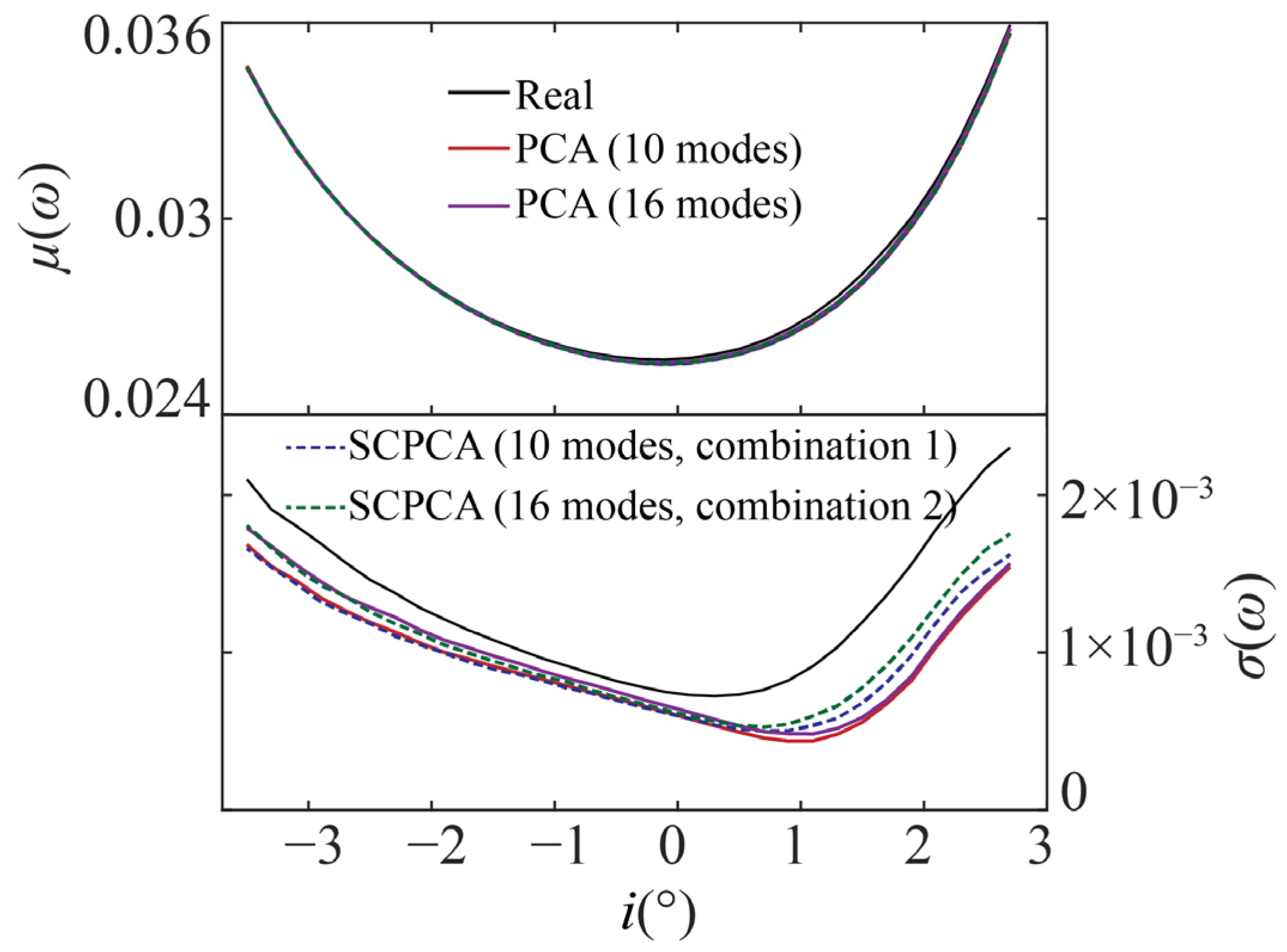
Figure 8 illustrates the variation of the mean and standard deviation of profile losses with respect to incidence for the 98 blade profiles reconstructed using the PCA and SCPCA methods. The solid black line in
Figure 8 represents the 98 real blade profiles. It can be observed that both PCA and SCPCA methods yielded accurate evaluations of the mean aerodynamic performance. However, the SCPCA method could improve the accuracy of evaluating the scatter of aerodynamic performance in positive incidence while maintaining the accuracy of evaluating the scatter in negative incidence. In particular, when reconstructing the 98 blade profiles using 16 modes, the SCPCA method improved the accuracy of evaluating the scatter of positive incidence range by 11.8% compared to the PCA method. This conclusion was drawn from the data of 98 blade profiles; however, similar to the results shown in
Figure 3, concern about the statistical convergence should be very critical. Hence, statistical inference methods and the commonly used Monte Carlo simulation methods were both employed to validate the superiority of the SCPCA method.
The interval estimation method was applied to overcome the difficulty of convergence for the statistical parameters in point estimation with 98 data. Calculating statistical parameters of the aerodynamic performance of all manufacturing blades from observable data is a statistical inference problem. There are two distinct types of estimation methods [
34]. The first is point estimation, which estimates the value of a population parameter using a certain number. This method is widely used because of its intuition. The second is interval estimation, which estimates a range of possible values of the population parameter. When point estimation is performed, often thousands of samples are necessary to achieve convergence [
19,
26,
35]. However, interval estimation does not require so many samples because increasing the sample size only changes the length of confidence interval (CI). When the samples have a normal distribution, there is an exact formula for calculating the CI of the mean value. Unfortunately, no efficient formula exists for other distributions, nor for most statistical parameters. In such cases, other methods must be used to calculate the interval. The bootstrap method is effective and precise for estimating CIs [
36]. DiCiccio and Efron [
37] compared various types of bootstrap method. For convenience, the percentile bootstrap method was used to calculate the CI with a 90% confidence level for all statistical performances. When calculating the 90% CI of the mean performance
of 98 real blades, resampling 98 blades with replacement was sufficient to calculate a new mean performance
. This procedure was repeated 2000 times to create 2000 means,
, which were then sorted by their values. A 90% CI for the mean performance
was determined by the new means
at the 5th and 95th percentiles. The same process can also be used to calculate 90% CI for the standard deviation of the parameters involved in evaluating blade aerodynamic performance.
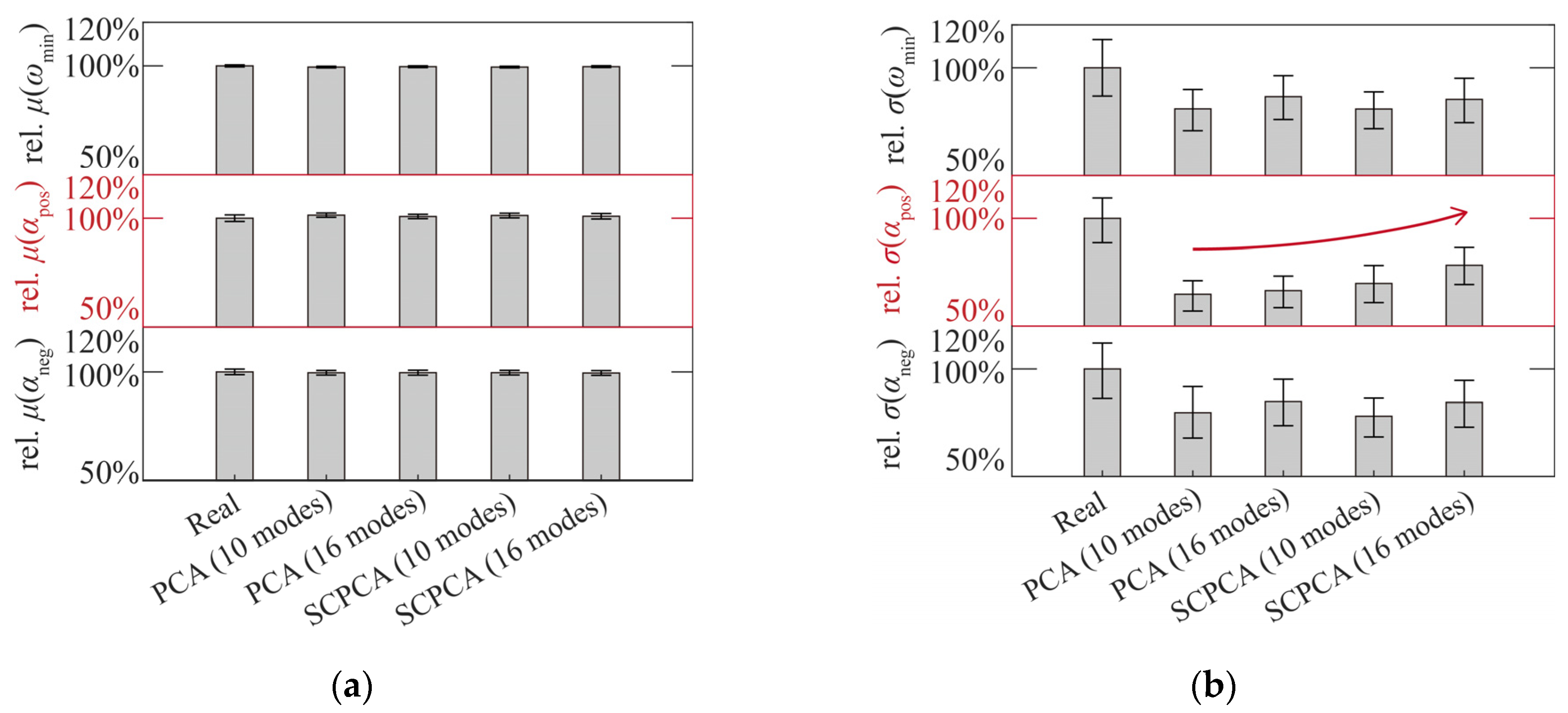
Figure 9 shows the statistical performances of different sets of blade profiles. All the statistical values were nondimensionalized using the data of the real blade profiles:
where
and
are the dimensionless mean value and standard deviation, and
and
denote the mean value and standard deviation of real blade profiles, respectively. In
Figure 9, the heights of the gray bars indicate the statistics estimated from the 98 blade profiles, whereas the error bars represent the 90% CIs generated using the bootstrap method. In
Figure 9a, for each blade set, the fluctuations corresponding to the 90% CI of the mean value are very small. This result shows that both the PCA and the SCPCA methods could provide a precise estimation of the blade mean performance. The wide CI in
Figure 9b indicates that accurately assessing the standard deviation for the parameters of the aerodynamic performance was more challenging than it was for the parameters of the mean performance. The advantage of the SCPCA method is evident (see
Figure 9b) as it can improve the accuracy for evaluating the scatter of positive incidence ranges while maintaining the accuracy for evaluating the scatter of other performance parameters. An noteworthy additional phenomenon is that both the PCA and the SCPCA methods tend to underestimate the scatter of blade performance when employing a small number of eigenmodes.
To demonstrate the advantage of the SCPCA method more clearly,
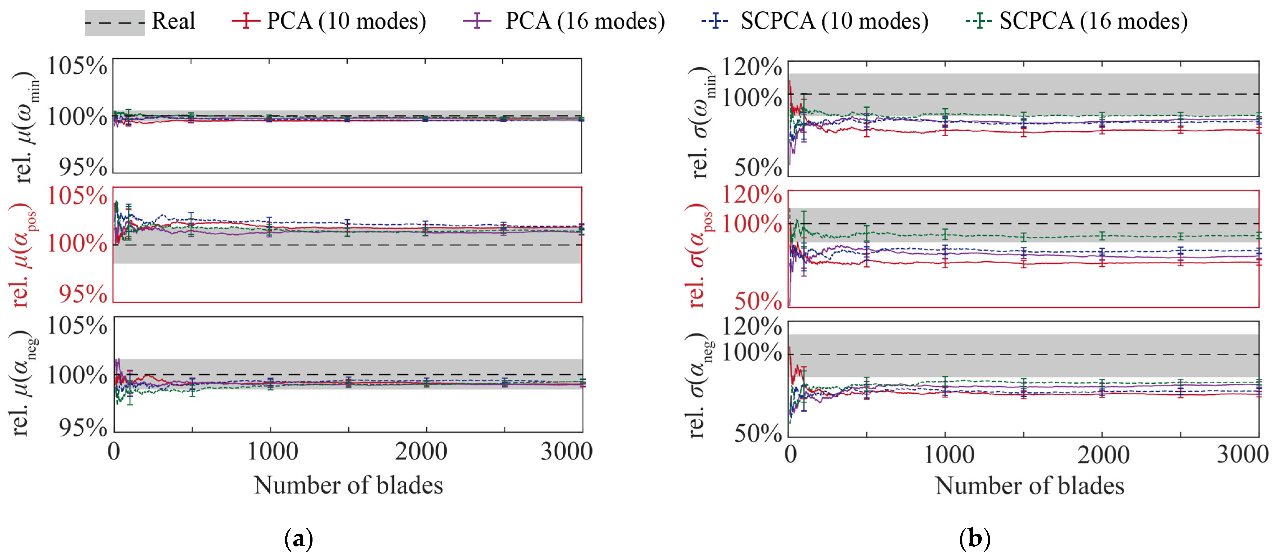
Figure 10 presents the statistical values and 90% CIs of blade aerodynamic performance parameters obtained from 3000 Monte Carlo samples of blade profiles generated using different modeling methods and modal numbers. It should be noted that during the process of generating random samples through the Monte Carlo simulation, it was assumed that the projection values of the samples on each mode followed a normal distribution. The black dotted line represents statistics from 98 real blade profiles with deviations. The grey shadow indicates the 90% CI of statistic results for the real blade profile acquired using the bootstrap method.
Figure 10 clearly confirms the same conclusion as drawn in the previous text; examining
Figure 10, it is evident that the SCPCA method (which utilizes only 10 modes) achieved a higher level of prediction accuracy than the PCA method (which uses 16 modes) in predicting the variability of compressor performance from the design condition to the near-stall condition. This is a matter of great concern for compressor designers as it is closely related to the compressor-stall margin. Thus, it can be said that the SCPCA method could employ fewer eigen modes to evaluate the variability of blade performance parameters at the same level of accuracy as when using the PCA method. In the field of UQ and robust design, an increase in the number of variables always results in an exponential increase in the number of simulations. For example, when the goal is to reduce performance uncertainty for a blade profile, the geometric deviation must be modeled to introduce uncertainty. If the PCA method requires 16 principal modes for deviation modeling, then 16 variables are introduced. By contrast, the SCPCA method requires fewer variables to solve this problem. Consequently, by immediately reducing the problem’s dimension, computational requirements could be significantly decreased. Therefore, the SCPCA method has a potential to reduce computational costs for future applications.
6. Working Mechanism for SCPCA
In order to determine the mechanism by which the SCPCA method achieves superiority when compared to the PCA method, the comparison of the detailed flows on 98 real blade profiles and 98 profiles reconstructed with 16 eigen modes using both the PCA and SCPCA methods were conducted. For the study of the flow on blade surfaces, the inlet incidence condition should first be carefully chosen. Although the critical positive incidence condition (i.e., the incidence with 1.5 times the minimum total pressure loss) varied among different blade profiles, the incidence of
was close to the critical positive incidence condition for most of the blade profiles, as shown in
Figure 3. Therefore, the flows at the incidence condition of
were compared for all blade profiles.
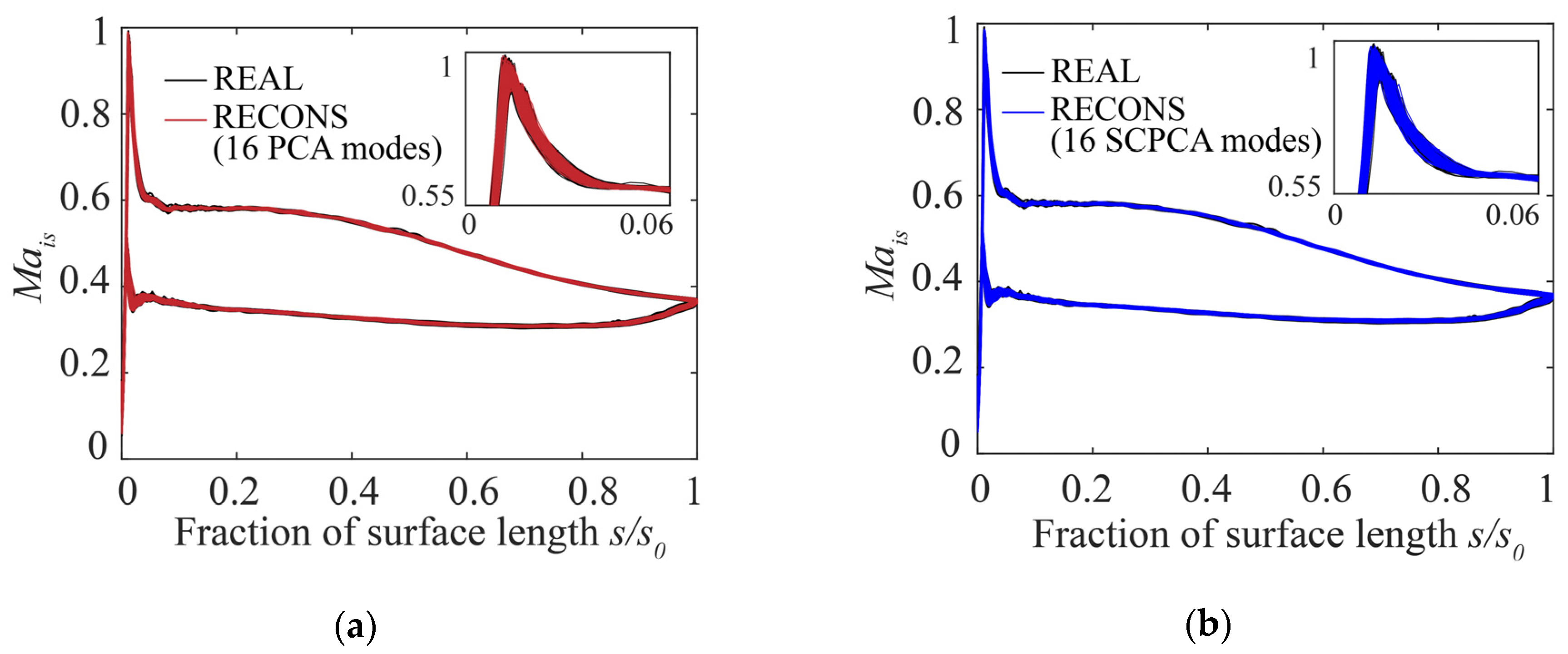
Figure 11 shows the isentropic Mach number
on different blade profiles. Different forms of deviations had little influence on the load distribution of blade profiles. The scatter of the isentropic Mach number was more severe near the spike around the LE than it was at other positions on the blade surface.
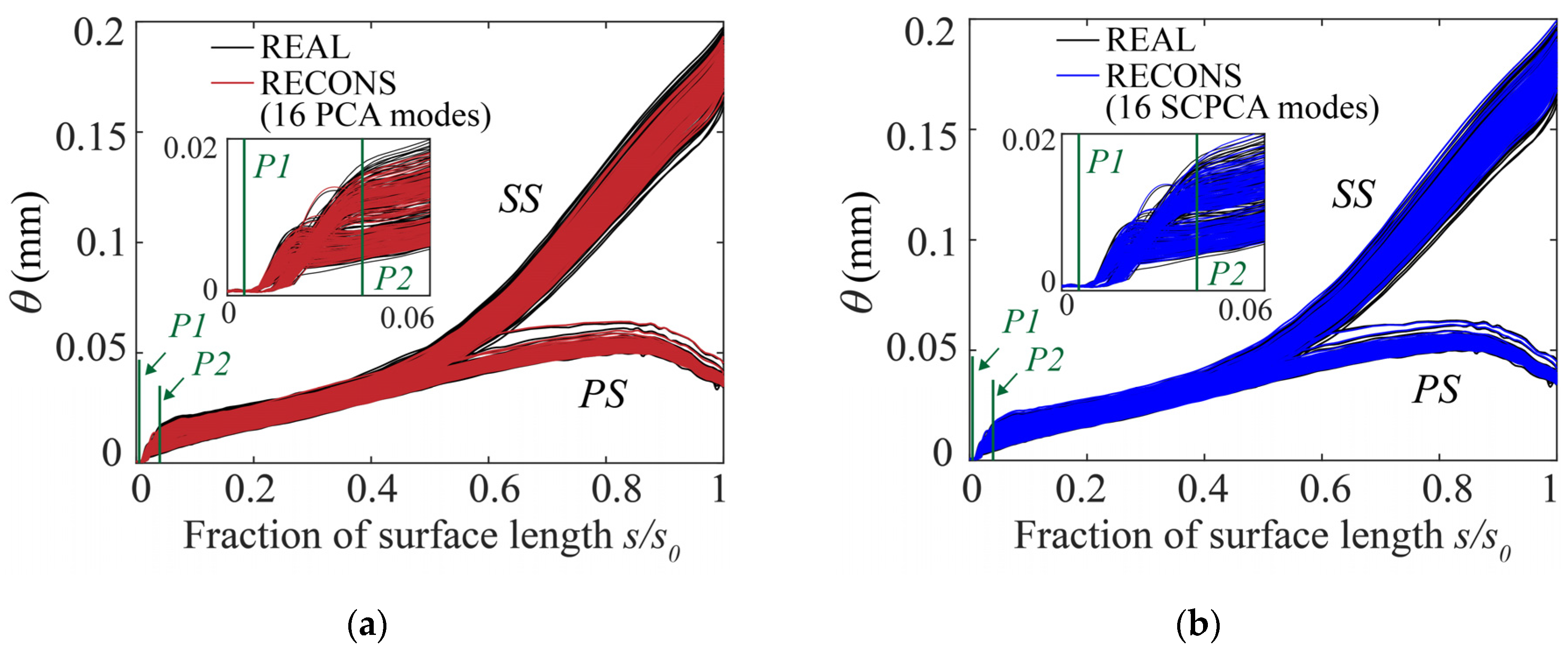
Figure 12 and
Figure 13 show the comparisons of the boundary layer momentum thickness
and shape factor
H.
Figure 12 illustrates that the large scatter of the boundary layer momentum thickness caused by the deviations occurred on the SS, for the analyzed positive incidence condition. As shown in
Figure 12a, the deviation near the LE (shown between positions of P1 and P2) greatly increased the scatter of the boundary layer momentum thickness. By contrast, the deviation downstream of P2 position had less of an impact on the boundary layer. The same phenomenon could also be observed in
Figure 12b.
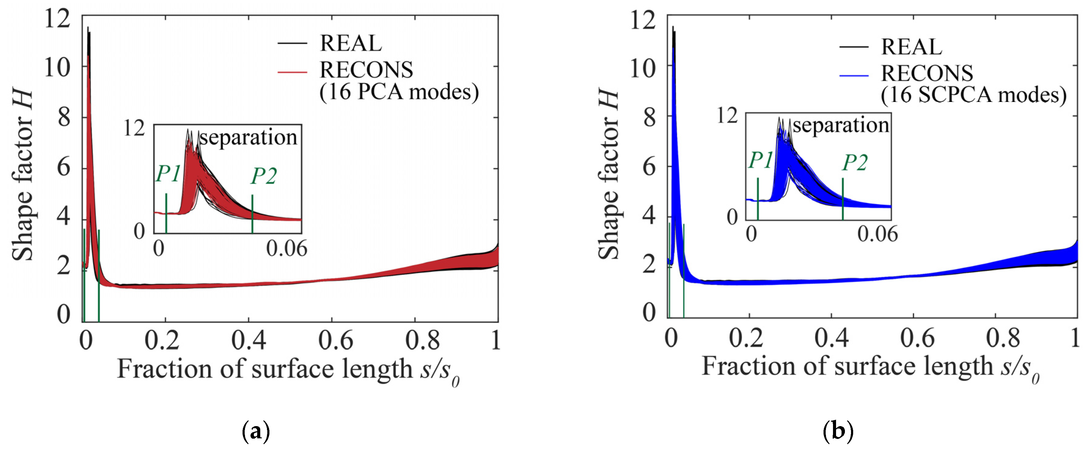
Figure 13 illustrates the boundary layer shape factor on the SS of different blade profiles. A separation bubble transition occurred at the LE for all blade profiles at the analyzed positive incidence condition, which could also be observed for the nominal blade profile. There was a significant scatter observed at the position of the shape factor’s peak, which was approximately 1% of the surface arc length downstream from the LE point. This phenomenon indicated that the transition behavior was sensitive to geometric disturbance, which was also found by Goodhand [
38].
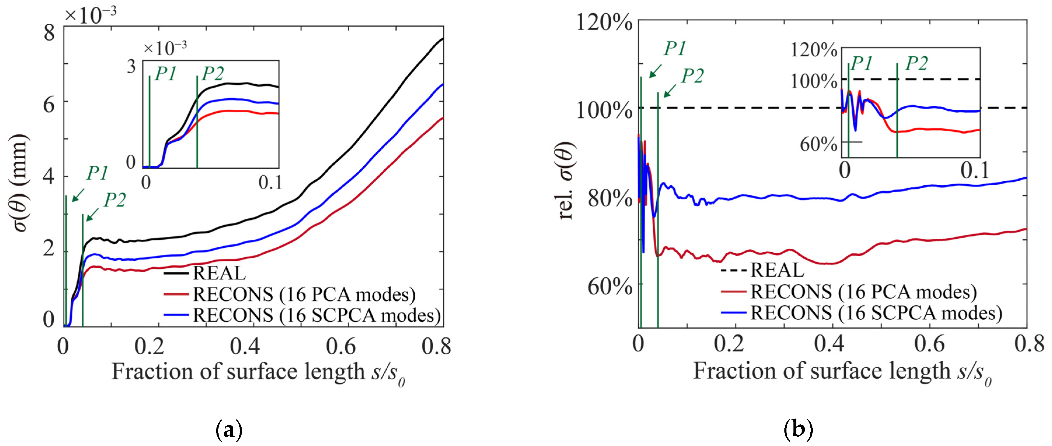
To further clarify the superiority of the SCPCA method for assessing the variance of the positive incidence range,
Figure 14a shows the variation of the standard deviation of the boundary layer momentum thickness along the suction surface for different blade sets at the incidence condition of
.
Figure 14b is the same as
Figure 14a, except the data has been normalized using the standard deviation of the boundary layer momentum thickness for the real blade profiles. In
Figure 14a,b, upstream of the location of boundary layer transition (i.e., about P2 position), the standard deviations of the momentum thickness obtained from the two reconstructed blade sets are nearly identical. Downstream of the end of separation bubble transition regions, the SCPCA method was able to evaluate a scatter of the boundary layer momentum thickness much closer to the real one. Evidently, the separation bubble transition at the leading edge had a geometric sensitive flow structure, which significantly influenced the aerodynamic performance of all calculated blade profiles. This sensitive flow structure is critical for the prediction of the positive incidence range, as shown in
Figure 6d. Due to the consideration of sensitive information in the SCPCA method, more attention was given on the modes which reflect the geometric variations in the regions where the sensitive flow structure occurs. As a result, the SCPCA method can provide a more accurate assessment of the scatter of the blade positive incidence range.
7. Conclusions
The PCA-based geometry deviation modeling method was widely used for the study of compressor performance UQ, sensitivity evaluation, and robust design. However, as the traditional PCA method is only a geometry-based method, while this method might have some missing modes with a small eigenvalue it possesses significantly more aerodynamic sensitivity. As a result, the PCA-based UQ usually underestimates the scatter of the compressor performance caused by blade geometry variations. To deal with this problem, a novel geometry deviation modeling method, named SCPCA, was proposed. Based on the SA result, weighting factors of deviation for each eigenmode were determined and then used to modify the process of PCA. As a result, the main eigenmodes (considering the covariance of geometry variation and performance sensitivity) could be determined and used to reconstruct the blade samples in the analysis of UQ or other related studies. The proposed SCPCA method was applied to real compressor rotor blades for deviation modeling compared with the PCA method. The errors of uncertainty evaluation induced by using different methods were quantified, and the working mechanism resulting in different assessing accuracies was investigated. Thus, the feasibility and effectiveness of the SCPCA method were verified. Conclusions can be drawn as follows:
The PCA and SCPCA methods were capable of accurately estimating the mean performance of real blade profiles. However, the standard deviation of aerodynamic performance is underestimated when either of the applied methods only uses a few modes.
In this analysis of the measured blades, using 16 modes for both of the SCPCA and PCA methods, the SCPCA method improved the predictive accuracy of the variability of the positive incidence range by 11.8%, while maintaining the same level of predictive accuracy for the variability of other performance parameters as the PCA method. Hence, for the same cost of computational resources, when compared to the traditional PCA method, the SCPCA method could achieve an overall improvement in predicting the performance variability of the compressor from the design condition to the near-stall condition.
With the same level of prediction accuracy for the compressor performance variability from the design condition to the near-stall condition (a factor which should be of concern to compressor designers, being related to the compressor stall margin), the SCPCA method has a potential to reduce computational costs significantly, when compared to the traditional PCA method.
The transition in the separation bubble was crucial for the assessment of performance variability. The SCPCA method could maintain the covariance relationships between coordinate points on the blade surface. In addition, by focusing on the area where sensitive flow structures exist, this method effectively improved the accuracy of variability evaluation of aerodynamic performance.
The results can provide a reference for further research on deviation modeling In turbomachinery. However, owing to data limitations, only 98 real blade profiles were analyzed. Future studies can shorten the CI of performance estimation by using more real blade profile data.


