Path Planning of an Unmanned Combat Aerial Vehicle with an Extended-Treatment-Approach-Based Immune Plasma Algorithm

Abstract

The increasing usage of unmanned aerial vehicles (UAVs) and their variants carrying complex weapon systems, known as unmanned combat aerial vehicles (UCAVs), has triggered a global revolution in complex military and commercial operations and has attracted researcher attention from different engineering disciplines in order to solve challenging problems regarding these modern vehicles. Path planning is a challenging problem for UAV and UCAV systems that requires the calculation of an optimal solution by considering enemy threats, total flight length, fuel or battery consumption, and some kinematic properties such as turning or climbing angles. In this study, the immune plasma (IP or IPA) algorithm, one of the most recent nature-inspired intelligent optimization methods, was modified by changing the default plasma transfer operations with a newly proposed technique called the extended treatment approach; extended IPA (ExtIPA) was then introduced as a path planner. To analyze the solving capabilities of the ExtIPA, 16 cases from five battlefield scenarios were tested by assigning different values to the algorithm-specific control parameters. The paths calculated with ExtIPA were compared with the paths found by planners on the basis of other intelligent optimization techniques. Comparative studies between ExtIPA and other techniques allowed for stating that the extended treatment approach significantly contributes to both the convergence speed and qualities of the obtained solutions and helps ExtIPA in performing better than its rivals in most cases.

1. Introduction

Tremendous advances in computing, communication, optical, weapon, and ammunition technologies have brought unexpected reconnaissance, surveillance, and destructive capabilities to unmanned aerial vehicles (UAVs) and unmanned combat aerial vehicles (UCAVs) [1,2]. To increase the likelihood of success of a task assigned to a UAV, UCAV, or similar modern aerial vehicle, a flight path should be carefully calculated by taking into account some optimization goals related to enemy threats, fuel consumption, or battery usage [3,4]. Even though graph-based algorithms such as the Voronoi diagram, A* search, D* lite, and other classical techniques such as rapidly exploring random trees (RRT), artificial potential fields (APF), and probabilistic road maps (PRM) are commonly used for calculating UAV or UCAV paths, they require the generation of cost maps of complex battlefields and usually suffer from convergence to local optimal solutions [5,6].

In recent years, meta-heuristic algorithms, which are a branch of artificial intelligence techniques, have started being used as path planners of UAV or UCAV systems because of their advantages regarding their implementation simplicity, computational complexity, and configurable or adjustable structures [7,8,9]. C. Xu et al. directed the employed foragers of the artificial bee colony (ABC) algorithm to the best current food source by utilizing chaotic variables for their path planner, named chaotic ABC (CABC), and pictorially proved the superiority of the CABC over the ABC algorithm [10]. Y. Zhang et al. converted the raw fitness values of food sources by using a fitness scaling strategy and employed Lorenz equations to generate random numbers required by the bee phases to improve the path-planning performance of the ABC algorithm [11]. In another study, Y. Zhang et al. improved the selection probabilities of qualified solutions by taking into account a fitness scaling mechanism for the particle swarm optimization (PSO) algorithm [12]. Moreover, Y. Zhang et al. adaptively adjusted the inertial weight and acceleration coefficients of the population update equation in PSO and utilized a chaotic random number generator to determine the values of the random coefficients of the same equation [12]. The PSO algorithm introduced by Y. Zhang et al., called the fitness-scaling adaptive chaotic PSO (FAC-PSO), was used as a path planner [12]. P. Li and Duan referenced the idea of memory and social information concept of PSO for their gravitational search algorithm (GSA), and its effectiveness on solving UAV path-planning problems was verified via comparisons with the standard PSO, GSA, and two other GSA-based models [13]. Fu operated a version of the PSO algorithm for which each particle modified the related velocities by guiding the best solution of a small solution group as the path planner [14].

G.-G. Wang et al. designed a new information-sharing approach between the qualified solutions of the firefly algorithm (FA) and presented the modified FA (MFA) [15]. A detailed comparison was presented between the MFA and other meta-heuristic-based UAV path planners such as PSO, ant colony optimization (ACO), differential evolution (DE), biogeograph-based optimization (BBO), evolutionary strategies (ES), population-based incremental learning (PBIL), genetic algorithm (GA), and, lastly, a variant of GA known as stud GA (SGA) [15]. The studies pioneered by G.-G Wang were not limited to the MFA. G.-G. Wang et al. tried to embed some dynamics of the DE algorithm into cuckoo search (CS), and the DE/CS algorithm was announced for planning UCAV paths being operated in a three-dimensional environment [16]. G.-G. Wang et al. altered the solution update procedure of the bat algorithm (BA) with the mutation operator of DE, and BAM was presented [17]. The qualities of the obtained UCAV paths allowed for stating that the mutation operator accelerated the convergence speed of BA while maintaining the existing strong search characteristics of the algorithm [17]. A separate study of G.-G. Wang et al. borrowed the mutation operator from the DE and ported it into the workflow of BA [18]. The BA with the support of the mutation operator of DE was named improved BA (IBA) and was tested in a three-dimensional environment to calculate optimal UCAV paths [18]. The BBO algorithm was updated with chaos theory and the predator–prey concept by W. Zhu and Duan; then, chaotic predator–prey BBO (CPPBBO) was introduced for solving path-planning problems [19]. These authors conducted a set of experiments for a UAV with constraints regarding the maximal yawing angle and flight length [19]. Heidari and Abbaspour varied the communication relationship between the stars and other elements of the black hole (BH) algorithm, and controlled the effects of modifications over UCAV path-planning problems [20]. Tang and Zhou replaced the location update model of glowworm swarm optimization (GSO) with the mechanism inherited from the PSO, and introduced the PGSO algorithm [21]. The performance of PGSO was analyzed in detail for path-planning problems, and it obtained more qualified solutions than other tested algorithms did, especially when the number of segmentation points or waypoints was set to 5 or 10 [21].

G. Yu et al. applied teaching–learning-based optimization (TLBO) to a two-dimensional UAV path-planning problem and reached some critical conclusions regarding the solving capabilities of TLBO compared with the ABC, PSO, DE, and GSO algorithms [22]. X. Zhang and Duan defined multiple constraints such as the total cruise length, flight altitude, turning angle, climbing or gliding slope, terrain, non-flight zones, and enemy threats, including radars, missiles, and anti-air guns, for path-planning problems; they announced a DE algorithm specialized with an $\alpha$-level comparison-based constraint-handling technique [23]. Q. Zhou et al. changed the wolf colony search (WCS) algorithm, so that the complex method was responsible for managing the leading strategy of the wolf colony; they simulated a newly proposed technique called CWCS as the path planner [24]. B. Li et al. first developed the balance-evolution strategy (BES) by controlling the trial counters of employed bees to generate candidate solutions in the ABC algorithm, and the BE-ABC algorithm was introduced [25]. They examined the BE-ABC algorithm for planning UCAV paths by using three different battlefield scenarios, and compared BE-ABC, ABC, and two ABC variants, namely, the I-ABC and IF-ABC algorithms [25]. The predator–prey concept was combined with the pigeon-inspired optimization (PIO) by B. Zhang and Duan, and predator–prey pigeon-inspired optimization (PPPIO) was presented [26]. They prepared test scenarios for which danger zones moved dynamically and planned UCAV paths with PPPIO [26]. Y. Zhou et al. specialized some stages of wind-driven optimization (WDO) with the quantum rotation gate and quantum non-gate strategies, and quantum WDO (QWDO) was proposed [27]. The UCAV paths found by QWDO were compared with the paths found by quantum-supported variants of PSO and BA, and standard implementations of the WDO, PSO, and DE algorithms [27].

S. Zhang et al. focused on how the standard implementation of the grey wolf optimizer (GWO) performs on calculating UAV paths for two-dimensional test cases [28]. Luo et al. represented the solution of BA with the quantum encoding and executed the quantum rotation gate to manage update operations and the quantum dot gate to manage the mutation operations for their path planner known as quantum encoding BA (QBA) [29]. Q. Zhang et al. decided to develop a collection decision optimization algorithm (CDOA)-guided technique and verified the effectiveness of it after solving the UAV path-planning problem [30]. Alihodzic et al. investigated the path-planning capabilities of the elephant herding optimization (EHO) algorithm for two-dimensional battlefields [31]. Alihodzic et al. also solved UCAV path-planning problem with the fireworks algorithm (FWA)-based approach in which the qualities of solutions are utilized for determining how many sparks are generated and how the exploitation amplitude is calculated [32]. Miao et al. provided an extensively rich set of experiments about their path planner developed via the hybridization of the simplex method (SM) and the symbiotic organism search (SOS) algorithm [33]. Dolicanin et al. configured the brain storm optimization (BSO) algorithm as a path planner and used a battlefield with five enemy threats for testing [34]. Pan et al. adjusted the scaling factor and fraction probability of the CS algorithm with the help of chaotic sequences of Circle-type Chaotic Maps and showed the superiority of their CS algorithm against the standard CS algorithm for solving the UCAV path-planning problem [35]. The valuable contribution to the literature of intelligent UAV or UCAV path-planning by the studies pioneered by Pan has carried over to current times. Pan et al. remodeled the process of encircling or searching for the prey of the whale optimization algorithm (WOA) with a self-tuning parameter based on the qualities of the agents [36]. Two battlefield scenarios were simulated with the purpose of UCAV path-planning, and it was understood that improved WOA achieves more qualified paths compared to the standard WOA [36]. Moreover, Pan et al. brought together the advantageous sides of two DE variants such as CIPDE and JADE, and CIJADE was proposed [37]. In CIJADE, the crossover rate and scaling factor were determined according to a parameter adaption strategy in each cycle or generation. Some tests carried out for a battlefield with ten enemy threats demonstrated that CIJADE outperforms PSO, DE, ABC, JADE, and CIPDE, and the superiority of CIJADE becomes more apparent when the number of segmentation points is increased [37].

Lin et al. altered the position update procedure of BA with the help of APF when designing a BA-guided path planner [38]. They also improved the inertia weight of the mentioned BA by using the optimal success rate strategy and chaos theory to further escape the local optimal solutions [38]. Qu et al. integrated reinforcement learning (RL) into the workflow of GWO by assuming that the population members of GWO correspond to the training agents of RL and introduced RLGWO for calculating optimal UAV paths [39]. RLGWO was tested using three battlefield scenarios and compared with the standard GWO and its variants, including IGWO, MGWO, and EEGWO [39]. The GWO algorithm was selected by Qu et al. in another study. They hybridized a simplified variant of the GWO algorithm with SOS that uses a modified commensalism phase and developed HSGWO-MSOS [40]. Comparative studies between HSGWO-MSOS, GWO, SOS, and simulated annealing (SA) conducted on both two- and three-dimensional scenarios proved the better performance of the newly proposed technique [40]. Monarch butterfly optimization (MBO) was modified by Yi et al. in a manner that quantum operators are responsible for regenerating a certain set of worst butterflies, and quantum-inspired MBO (QMBO) was proposed as a three-dimensional path planner [41]. C. Wu et al. considered some physical constraints of the UAV when exploring the search space and used them in the initialization of the bees belonging to ABC algorithm [42]. Yang Chen et al. changed the global update equation of the flower pollination algorithm (FPA) to guarantee a non-monotonic decreasing sequence [43]. In addition to this, a population reconstruction mechanism was added to protect the algorithm from premature convergence [43]. The new implementation of the FPA, named neighborhood global-learning-based FPA (NGFPA), was executed to find optimal UAV paths, and its results were compared with the results of some well-known techniques such as A*, APF, and RRT [43].

H. Zhu et al. provided a detailed comparative study by using standard versions of ABC, BA, DE, FA, GWO, PSO, WOA, CS, a modified variant of MBO called GSMBO, harmony search (HS) and spider monkey algorithm (SMA) and concluded that SMO is able to planning more safe UCAV paths than other tested algorithms do [44]. The superior performance of SMO gave inspiration to H. Zhu et al. for developing new path planners on the basis of the mentioned algorithm. The SMO supported with cooperative co-evolution, which is a method helping the division of the parameter set into smaller sub-sets first to solve them independently and then combining the partial solutions appropriately, was used by H. Zhu et al. when planning UCAV paths [45]. In order to validate the competitiveness of the SMA-based technique, twenty-five cases under five different scales were described and tested [45]. X. Zhou et al. tried to handle the poor local search ability of BA with the help of the ABC algorithm, and the improved BA (IBA) was presented and tested for planning UAV paths in an environment containing specially modeled enemy radars, missiles, anti-aircraft weapons, and climate effects [46]. P. Wu et al. determined the values of the random coefficients in the PSO algorithm using a Zaslavskii chaos map, and a path planner named improved chaotic PSO was announced [47]. H. Xu et al. remodeled the critical sections of the GSA by using an adaptive alpha-adjusting strategy and a Cauchy mutation strategy. The GSA variant, also called mixed-strategy-based GSA (MSGSA for short) was used to obtain optimal UAV paths by considering enemy threats, total flight length, turning angles, and non-flight zones [48].

One of the most specialized UAV path planners was introduced by Jiang et al. at the beginning of 2022 [49]. They changed the workflow of the standard GWO by adding a communication mechanism for avoiding local optimum solutions in the search process and $ϵ$-level comparison for managing constraints [49]. Moreover, they utilized the partially observable Markov decision process and Monte Carlo tree search algorithm for the purpose of collision avoidance [49]. X. Wang et al. supported different stages of the mayfly algorithm (MA) and offered the modified MA (modMA) [50]. In the modMA, the gravity coefficient was determined with an exponent inertia weight strategy, and the position of each male mayfly was adjusted by employing Cauchy-based mutation approach [50]. Finally, they integrated the horizontal crossover strategy in which the solution space is divided into hypercubes to allow the parent individuals to generate candidates of distant regions [50]. Niu et al. controlled different stages of the artificial ecosystem optimizer (AEO) and proposed an adaptive neighborhood-based search-enhanced AEO (NSEAEO for short) to address the UCAV path planning problem [51]. In NSEAEO, distance-fitness-based information was used to define neighborhoods for consumers and a significant contribution was given to the global exploration capability of the algorithm [51]. Moreover, Niu et al. employed a novel decomposition method maintaining the population diversity. Experimental studies on both two- and three-dimensional environments showed that NSEAEO is able to handle challenging objectives regarding enemy threats, total flight length, and turning and climbing angles more robustly than other techniques can, such as the salp swarm algorithm (SSA), the stain bowerbird optimizer (SBO), the pathfinder algorithm (PFA), the sine–cosine algorithm (SCA), two PSO variants named GAPSO and CIPSO, GA, MFO, a modified TLBO (ECTLBO), HSGWO-MSOS, and AEO [51]. Jia et al. developed a new approach called double-layer coding (DLC) used for deciding which segmentation points or waypoints are considered to define a UCAV path and used it with their PSO variant known as rotation-based PSO (RPSO) [52].

When the details given about a how a meta-heuristic algorithm is specialized or modified in order to solve UAV or UCAV path-planning problem are given, it can be easily seen that nature has a tremendous potential to inspire researchers in the development of new computational intelligence techniques. The immune plasma algorithm (IP algorithm or IPA) is one of the most recent meta-heuristic methods that shows the immense richness of nature by modeling the fundamental steps of a medical method. This algorithm gained popularity again with the COVID-19 pandemic and was named as the convalescent or immune plasma treatment [53]. If the main operations executed by the IPA are investigated, it can be easily seen that the IPA differs from the most representative meta-heuristics including ACO, ABC, PSO, BA, FA, FWA, DE, and GA [53]. While the exploitation-dominant operations of the IPA are designed in a semi-adaptive manner and adjust the convergence dynamically without changing the initial values of the control parameters, a quasi-deterministic approach is responsible for managing the important part of exploration, and its promising performance has been validated recently for engineering problems such as channel assignment [54], time series prediction [55], wireless sensor deployment [56], signal noise minimization [57], neural network training [58], and also UAV or UCAV path planning [59]. In this study, the plasma transfer scheme of the IP algorithm was changed with a newly introduced approach called extended treatment, and an extended IP algorithm, or ExtIPA, was designed to solve the path-planning problem. The extended treatment approach mainly depends on continuing the transfer of plasma from the donor to the selected receiver until the receiver becomes better than its donor and allows for the algorithm to search the vicinity of the eligible solutions more sensitively. The contribution of the extended treatment approach on the qualities of planned UCAV paths was investigated by using different battlefield scenarios, and obtained solutions were compared with the solutions of other meta-heuristic-based path planners. Comparative studies between ExtIPA and other techniques showed that the newly introduced treatment approach significantly improves the exploitation performance of the IPA while maintaining the existing exploration capabilities, and ExtIPA outperforms its competitors in most of the test cases. The rest of the paper is organized as follows: Details of the path-planning problem and score calculation method are given in Section 2. Fundamental steps of the IP algorithm are summarized in Section 3. Section 4 is devoted to the extended treatment approach and its integration into the IPA. The results of the experiments and comparative studies are presented in Section 5. Finally, some conclusions and future works about the development of new IPA-based path planning techniques are mentioned in Section 6.

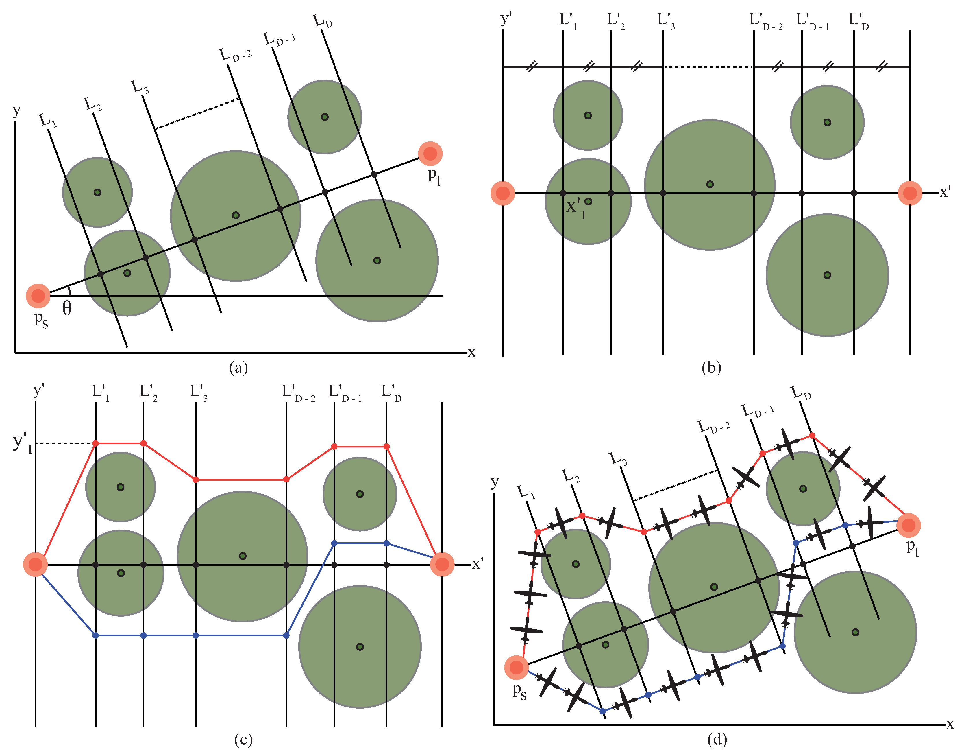
2. Mathematical Description of the UCAV Path-Planning Problem

Before we start to determine a UCAV path, a strong mathematical model that describes enemy threats and their effects, the fuel or battery consumption over the total flight length, and a score calculation schema to understand how the path is qualified should be introduced. One of the commonly used mathematical models depends on describing an enemy threat by utilizing the radius of a circle with a known center coordinate to show the effect range and the grade or level to show the destructive capability. Given that there is a UCAV being planned to destroy a target positioned at $P_t=(x_t,y_t)$ by taking off from the start point at $P_s=(x_s,y_s)$, a reference line between $P_s$ and $P_t$ is drawn. Moreover, the reference line between $P_s$ and $P_t$ is divided equally into $D+1$ segments with the help of D segmentation points [59]. Each segmentation point on the reference line is intersected with a line that is vertical to the reference line, such as $L_1$ for point $P_1$ and $L_2$ for point $P_2$; then, line set $L=\{L_1,L_2,\dots ,L_{D-1},L_D\}$ is obtained. Set L serves a critical function in determining a flight path. Assume that only one point is selected from each line in the set L and combined appropriately with $P_s$ and $P_t$; then, a set of points described as $P=\{P_1,P_2,\dots ,P_{D-1},P_D\}$ can be generated. When each subsequent pair of points in set P is connected with a line segment, a UCAV path from start point $P_s$ to the target point $P_t$ can also be found [59].

Even though the forming a UCAV path by connecting each subsequent pair of points with a line segment seems relatively straightforward, finding the members of the set L and determining the coordinates of points in the set P require difficult calculations. To simplify the required calculations when generating the set L and set P, some properties of a new coordinate system in which the reference line corresponds to the horizontal axis can be utilized [59]. In order to transform a point of the original coordinate system into the appropriate counterpart of the new coordinate system, Equation (1) can be used [59]. While $x_k$ and $y_k$ are matched with the x-axis and y-axis values of point $P_k$ in the original coordinate system, ${\acute{x}}_k$ and ${\acute{y}}_k$ are matched with the $\acute{x}$-axis and $\acute{y}$-axis values of the transformed $P_k$ or ${\acute{P}}_k$ in Equation (1). $\theta$ is the angle between the x-axis of the original coordinate system and reference line and can be calculated as the results of the $arctan((y_s-y_t)/(x_s-x_t))$ operation [59]:

$$\left[\begin{array}{c}{\acute{x}}_k\\ {\acute{y}}_k\end{array}\right]=\left[\begin{array}{cc}cos\left(\theta \right)& sin\left(\theta \right)\\ -sin\left(\theta \right)& cos\left(\theta \right)\end{array}\right]\times \left[\begin{array}{c}{x}_k-x_s\\ y_k-y_s\end{array}\right]$$

(1)

Because the reference line becomes the horizontal axis of the new coordinate system and is divided equally into $D+1$ segments with D different segmentation points, the distance between two subsequent segmentation points is found equal to $|P_s{P}_t|/(D+1)$, and the ${\acute{x}}_k$-axis value of the ith segmentation point or ${\acute{x}}_i$ is also found equal to $i|P_s{P}_t|/(D+1)$ [59]. As stated earlier, each segmentation point is intersected with a line vertical to the reference line, and a point is selected from this vertical line. Considering the vertical line passing through the ith segmentation point, the $\acute{x}$-axis value of any point being selected from this line becomes equal to $i|P_s{P}_t|/(D+1)$, and only the $\acute{y}$-axis value is required [59]. If only the $\acute{y}$-axis values of the points being selected from the vertical lines are considered and organized in a set such as $\{{\acute{y}}_1,{\acute{y}}_2,\dots ,{\acute{y}}_{D-1},{\acute{y}}_D\}$, path planning can be turned into a problem for which the $\acute{y}$-axis values of D different points are optimally determined by selecting one for each vertical line with the purpose of a safe and efficient flight mission. A visual investigation can be conducted in order to understand the relationship between the original and transformed coordinate systems by controlling the Figure 1.

The geometrical modeling of the path-planning problem allows one to find an infinite set of possible solutions due to the continuous search spaces of the points. In order to compare two possible solutions to decide which path is better, a quality or score measurement schema should be described. A quality or score measurement schema used for comparing different paths is introduced in Equation (2) [59]. In Equation (2), $J_t$ is used to represent the cost of enemy threats for the considered path, and it is calculated using the integral of $w_f$ from 0 to the total length of the path, abbreviated as l. Similarly, $J_f$ is used on behalf of the cost of fuel consumption, and it is calculated using the integral of $w_f$ from 0 to the total length of the path. To adjust the weights of $J_t$ and $J_f$ in the construction of the J score, a constant called $\lambda$, chosen between 0 and 1, is directly multiplied by $J_t$, and the value of $1-\lambda$ operation is multiplied by $J_f$ [59].

$$J=\lambda J_t+(1-\lambda )J_f=\lambda {\int }_0^l{w}_{t}dl+(1-\lambda ){\int }_0^l{w}_{f}dl$$

(2)

The integral calculations about the cost of enemy threats and cost of fuel consumption can be carried out by using some approximations with acceptable accuracies. Given that $w_f$ is set to a constant such as 1, the $J_f$ is found to simply equal the length of the flight path [59]. If the length of the flight path increases, it is seen that the cost of fuel consumption also increases, as expected. When calculating the cost of enemy threats, integral-based operations are replaced with an approximation model in which the whole path is first divided by considering the subsequent points in the set P, and then each line segment is evaluated to understand whether it is in the effect ranges of enemy threats or not. Assume that $P_i$ and $P_j$ are two subsequent points, and the length of the path segment between these points is shown as $L_{ij}$. The path segment of length $L_{ij}$ is divided into ten subsegments and the first, third, fifth, seventh, and ninth subsegmentation points are named points $0.1$, $0.3$, $0.5$, $0.7$, and $0.9$. If the mentioned path segment is in the effect range of the kth enemy threat of grade $t_k$, the cost of the kth enemy threat on the path segment between $P_i$ and $P_j$ or $J_{t,\left(ij\right),k}$ is determined with Equation (3) [59]. In Equation (3), while $d_{0.1,i,k}^4$, $d_{0.3,i,k}^4$, and $d_{0.5,i,k}^4$ show the Euclidean distances between the center of the kth enemy threat and $0.1$, $0.3$, and $0.5$ subsegmentation points, $d_{0.7,i,k}^4$ and $d_{0.9,i,k}^4$ correspond to the Euclidean distances between the center of the kth enemy threat and $0.7$ and $0.9$ subsegmentation points. When the cost of all enemy threats are determined for each path segment and then summed, the value of $J_t$ can be obtained. As easily seen from the calculation details of $J_t$ and $J_f$ values, qualified paths have smaller J scores compared to other paths of the same battlefield [59].

$$J_{t,\left(ij\right),k}=\frac{L_{ij}{t}_k}{5}(\frac{1}{d_{0.1,i,k}^4}+\frac{1}{d_{0.3,i,k}^4}+\frac{1}{d_{0.5,i,k}^4}+\frac{1}{d_{0.7,i,k}^4}+\frac{1}{d_{0.9,i,k}^4})$$

(3)

3. Immune Plasma Algorithm

The new coronavirus, or COVID-19, first seen in Wuhan, China, at the beginning of 2019, caused a global health crisis that still affects people all over the world, and different medical methods and treatment approaches were developed in response. Immune or convalescent plasma treatment, used previously for the 1918 great influenza pandemic, also became a promising medical method for COVID-19. The idea behind this mentioned treatment approach that is over a hundred years old is transferring the blood and antibodies in the blood from an individual recovered recently to a critically ill patient. When the biologically strong idea lying behind the immune or convalescent plasma treatment is investigated from the viewpoint of a computer scientist, it is easily seen that there is an analogy with the transfer of blood from the selected donor to the critical patient and the exploitation of dominant operations of a meta-heuristic algorithm [53]. Aslan utilized the described analogy and introduced an IP algorithm (IPA for short) to the literature of artificial intelligence techniques [53]. When a problem that requires searching for optimal values for a set of decision parameters by considering the minimization or maximization of an objective function is attempted to be solved using IPA, a person or individual corresponds to a solution and the antibody amount or immune response of this individual is measured by using the objective function. If the IP algorithm decides that an individual in the population is a critical patient, or receiver, it selects another individual from the same population as a plasma donor, and treatment is started. Until the IPA completes a run because it reaches the maximum evaluation number or satisfies a similar termination criterion, the distribution of the infection between all members of the population, the selection of receiver and donor individuals, and the application of plasma treatment are carried out in a circular manner.

3.1. Generating Initial Members of the Population

The IP algorithm employs a randomized generation schema to determine initial values of its population members. Given that the problem being solved has D different parameters, the IP algorithm will start subsequent operations with a population of size $PS$. When representing an individual or member of population, a D-dimensional vector is used. By assuming that $x_k$ is the kth member of the population and $x_{kj}$ is the jth element or parameter of the mentioned individual, Equation (4) given below is executed in the IP algorithm with the purpose of assigning the initial value of $x_{kj}$ [53]. In Equation (4), $x_j^{max}$ and $x_j^{min}$ are problem-dependent upper and lower bounds for the jth parameter. $rand(0,1)$ also corresponds to a random number generated between 0 and 1 [53].

$$x_{kj}=x_j^{min}+rand(0,1)(x_j^{max}-x_j^{min})$$

(4)

3.2. Distributing Infection within a Population

Each member or individual of the population in the IPA is matched with a possible solution to the considered problem. When the initialization of individuals is completed, the IPA starts to distribute infection using a relatively simple model, as described in Equation (5), where $x_{kj}$ and $x_{mj}$ are used to represent the randomly selected jth parameters of $x_k$ and $x_m$ individuals, respectively [53]. $x_k^{inf}$ corresponds to the $x_k$ individual infected by the $x_m$, which is also chosen randomly from the population of size $PS$. $x_{kj}^{inf}$ represents the jth parameter of $x_k^{inf}$ newly calculated with the transmission of infection. Because $x_k^{inf}$ indicates the infectious $x_k$ individual, all of its parameters, except the jth one, are the same as the parameters of $x_k$ individuals. Finally, in Equation (5), $rand(-1,1)$ is matched with a random number generated between −1 and 1.

$$x_{kj}^{inf}=x_{kj}+rand(-1,1)(x_{kj}-x_{mj})$$

(5)

An infection triggers the immune system of the host, and a specific immune response in terms of the synthesized antibodies is given. To measure the level of a given response by an infectious individual, the IP algorithm directly utilizes the objective function of the problem [53]. When the IP algorithm tries to solve a minimization problem with the objective function f, the immune response or level of antibodies is determined as $f\left(x_k\right)$ for the $x_k$ individual before the infection and $f(x_k^{inf})$ for the $x_k$ individual immediately after the infection. If $f\left(x_k\right)$ is higher than $f(x_k^{inf})$, it is decided that the $x_k$ individual and its immune system is strong enough to handle the infection and the immune memory of $x_k$ should be updated for subsequent infection cycles by changing $x_{kj}$ to $x_{kj}^{inf}$. Otherwise, the $x_k$ individual remains unchanged, as described in Equation (6) [53].

$$x_{kj}=\left\{\begin{array}{cc}{x}_{kj}^{inf},& if f(x_k^{inf})<f\left(x_k\right)\\ x_{kj},& otherwise\end{array}\right\}$$

(6)

3.3. Treatment of Receivers with Donors

The IP algorithm continues the distribution of the infection until all population members meet with the infection. When all of the individuals meet with the infection, the IPA is ready to start its second main phase in which one or more individuals are treated by the support of one or more individuals chosen from the same population. In order to decide how individuals will be chosen as critical and labeled as receiver and how individuals will be chosen as recovered and labeled as donor, the IPA introduces two specific control parameters called $NoR$ and $NoD$ [53]. $NoR$ is the number of receivers, and the $NoR$ individuals who are worse than the remaining members are selected as receivers. The $NoD$ abbreviation is used on behalf of number of donors, and the $NoD$ individuals who are better than the remaining members are selected as donors. Assume that $x_k^{rcv}$ is the kth receiver from the set of receivers with the $NoR$ individuals and $x_m^{dnr}$ is the randomly selected donor from the set of donors with $NoD$ individuals. To model the transfer of a single plasma dose, Equation (7) is used by the IP algorithm [53]. In Equation (7), $x_{kj}^{rcv}$ and $x_{mj}^{dnr}$ show the jth parameters of $x_k^{rcv}$ and $x_m^{dnr}$, and j is selected from the set $\{1,2,\dots ,D\}$ sequentially. Moreover, $x_{kj}^{rcv-p}$ is matched with the jth parameter of $x_k^{rcv-p}$, and $x_k^{rcv-p}$ is used to represent the $x_k^{rcv}$ after transferring a single dose of plasma. If $f(x_k^{rcv-p})$ is less than $f(x_m^{dnr})$ for the first dose of plasma, $x_k^{rcv}$ is updated with $x_k^{rcv-p}$ appropriately, and treatment is continued, with the second dose taken from the same donor [53]. Otherwise, it is decided that the treatment does not cause a dramatic improvement in the immune system of $x_k^{rcv}$ and it should be completed. However, in order to guarantee that at least one dose of plasma is given, $x_k^{rcv}$ is updated with $x_m^{dnr}$, and treatment is concluded immediately after the first dose [53].

$$x_{kj}^{rcv-p}=x_{kj}^{rcv}+rand(-1,1)(x_{kj}^{rcv}-x_{mj}^{dnr})$$

(7)

The second and other doses of plasma are transferred to $x_k^{rcv}$ from $x_m^{dnr}$ by referencing the model introduced in Equation (7). However, the IPA changes the decision mechanism for understanding whether the plasma treatment is continued with a third dose of plasma or not. If $f\left(x_k^{rcv-p}\right)$ corresponding to the antibody level of $x_k^{rcv}$ after the second dose of plasma is less than the antibody level of $x_k^{rcv}$ after the first dose of plasma, $x_k^{rcv}$ is updated by using $x_k^{rcv-p}$, and then the treatment of $x_k^{rcv}$ is continued with a third dose of plasma from $x_m^{dnr}$ [53]. Otherwise, treatment is concluded for $x_k^{rcv}$, and the next receiver is selected, if they exist.

3.4. Modification of Donor Individuals

The antibody amount synthesized for a specific infection by the immune system of an individual recovered previously can decrease with time or incidence of encountering the infection. To model this type of change, the IP algorithm utilizes a random number generated between 0 and 1 and the ratio between $t_{cr}$ and $t_{max}$ [53]. Moreover, $t_{cr}$ is used to represent the current evaluation number, and it is increased by one for each evaluation. $t_{max}$ is used on behalf of the maximum evaluation number, and the IPA terminates when $t_{cr}$ becomes equal to $t_{max}$ [53]. If the ratio between $t_{cr}$ and $t_{max}$ is less than the generated random number, $x_m^{dnr}$ is reinitialized by using Equation (4) to indicate that the immune memory of the mentioned donor individual is not strong enough to synthesize the required amount of antibodies quickly [53]. Otherwise, $x_m^{dnr}$ donor individual is changed slightly, as described in Equation (8), where the j index ranges from 1 to D [53]. When the IP algorithm continues its run, $t_{cr}/t_{max}$ reaches 1, and the probability of generating a random number between 0 and 1 less than $t_{cr}/t_{max}$ increases intrinsically. As an expected result of this situation, the probability of using Equation (8) also increases, and the IPA tries to protect the immune memories of its donors. After executing the update procedure for all donors, the infection cycle of the IPA is completed and a new one is started.

$$x_{mj}^{dnr}=x_{mj}^{dnr}+rand(-1,1)x_{mj}^{dnr}$$

(8)

4. Details of Extended Treatment Approach

The treatment schema modeled in the standard implementation of the IP algorithm guarantees that a poor solution corresponding to a receiver is replaced with a solution represented by the selected donor or a solution better than the solution represented by the selected donor when the plasma transfer is completed. If the first dose of plasma cannot provide a satisfactory contribution and the receiver for which the first dose of plasma is given does not match to a solution better than the solution represented by its donor, the treatment is simply ended after replacing the receiver with a copy of the selected donor. Even though the idea underlying the used treatment schema brings some advantages to the IP algorithm, the possibility of copying the same donor more than once should be taken into account. When the treatment of receivers is completed by copying the same donor more than once, the population can have difficulties in managing solution diversities. Moreover, in the subsequent infection cycle, the chance of selecting the previously utilized donor and its copies also increases, and the IP algorithm requires a subtle configuration for the $NoR$ and $NoD$ parameters in order to handle the possible drawbacks stemming from the existing workflow of the plasma treatment.

The performance of the IP algorithm can be further improved by remodeling how the plasma from the donor will be transferred to the receiver and when the treatment will be completed. The requirement of $NoR$ or $NoD$ parameters and setting them appropriately can be removed completely if the exploitation characteristics of the newly designed plasma transfer and treatment operations are configured subtly. Given that $x_k^{rcv}$ is the kth receiver from the set of critical individuals of size $NoR$ and $x^{dnr}$ is the best individual of the entire population, when transferring the plasma from the $x^{dnr}$ to the $x_k^{rcv}$ individual, it is assumed that all of the parameters belonging to the $x^{dnr}$, except the randomly determined jth one, are copied into the $x_k^{rcv}$ and then jth parameter of the $x_k^{rcv}$ is calculated with the Equation (9) after plasma treatment is concluded. In Equation (9), $x_{kj}^{rcv-p}$ corresponds to the jth parameter of $x_k^{rcv-p}$ and $x_k^{rcv-p}$ is used on behalf of the $x_k^{rcv}$ individual who receives a dose of plasma from the donor.

$$x_{kj}^{rcv-p}=x_j^{dnr}+rand(-1,1)(x_j^{dnr}-x_{kj}^{rcv})$$

(9)

Standard implementation of the IP algorithm compares the antibody amount of $x_k^{rcv}$ immediately after the first dose of plasma calculated as $f(x_k^{rcv-p})$ with the antibody amount of $x^{dnr}$ calculated as $f(x^{dnr})$. For a minimization problem, if $f(x_k^{rcv-p})$ is not less than $f(x^{dnr})$, in other words, $x_k^{rcv-p}$ is not better than $x^{dnr}$, and $x_k^{rcv}$ is replaced with a copy of $x^{dnr}$ and treatment is ended. The replacement of $x_k^{rcv}$ with a copy of $x^{dnr}$ ensures that $x_k^{rcv}$ or a poor solution corresponding to $x_k^{rcv}$ is discarded from the population and a more qualified solution represented by $x^{dnr}$ is added. However, it should be noticed that some difficulties about the population diversity and efficiency of the subsequent treatment operations can be encountered and solving performance of the IP algorithm can deteriorate. In order to handle the possible problems to do with the replacement procedure between $x_k^{rcv}$ and $x^{dnr}$ individuals, an extended treatment approach that repeats the same plasma transfer operations as modeled by guiding Equation (9) until the $x_k^{rcv-p}$ becomes better than the $x^{dnr}$ is developed. By using the extended treatment approach, the IP algorithm empowers its exploitation characteristics because of the repetitive search in the neighborhood of the selected donor without requiring neither $NoD$ parameter nor its sensitive configuration. Newly proposed treatment approach allows IP algorithm to guarantee that $x_k^{rcv}$ will be replaced with a solution better than the solution represented by $x^{dnr}$. The IP algorithm that transfers plasma from the best individual in the population or $x^{dnr}$ to the $x_k^{rcv}$ in the receiver set of size $NoR$, as described by Equation (9), and continues plasma transfer until the receiver becomes better than its donor is called extended IPA for short ExtIPA. The details of treatment operations in ExtIPA can be controlled over the Algorithm 1.

Algorithm 1 Fundamental steps of extended treatment approach

1: $x^{best}\leftarrow$ get the best solution found so far  2: $rcvIndexes[1\dots NoR]\leftarrow$ get the indexes of the receivers  3: for   $i\leftarrow 1\dots NoR$  do  4:     $x^{dnr}\leftarrow$ get the best individual in the population as donor  5:     $k\leftarrow rcvIndexes\left[i\right]$ and determine $x_k^{rcv}$ as the current receiver  6:     if $t_{cr}<t_{max}$ then  7:         $t_{cr}\leftarrow t_{cr}+1$  8:         $x_k^{rcv-p}\leftarrow$ apply plasma treatment to $x_k^{rcv}$ with $x^{dnr}$ using Equation (9)  9:         while $f(x_k^{rcv-p})>f(x^{dnr})$ do 10:             if $t_{cr}<t_{max}$ then 11:                 $t_{cr}\leftarrow t_{cr}+1$ 12:                 $x_k^{rcv-p}\leftarrow$ apply plasma treatment to $x_k^{rcv}$ with $x^{dnr}$ using Equation (9) 13:             else 14:                 Terminate the run and send $x^{best}$ as the final solution 15:             end if 16:         end while 17:            Update $x_k^{rcv}$ with $x_k^{rcv-p}$ 18:         if $f(x^{best})>f(x_k^{rcv})$ then 19:             Update $x^{best}$ with $x_k^{rcv}$ 20:         end if 21:     else 22:         Terminate the run and send $x^{best}$ as the final solution 23:     end if 24: end for

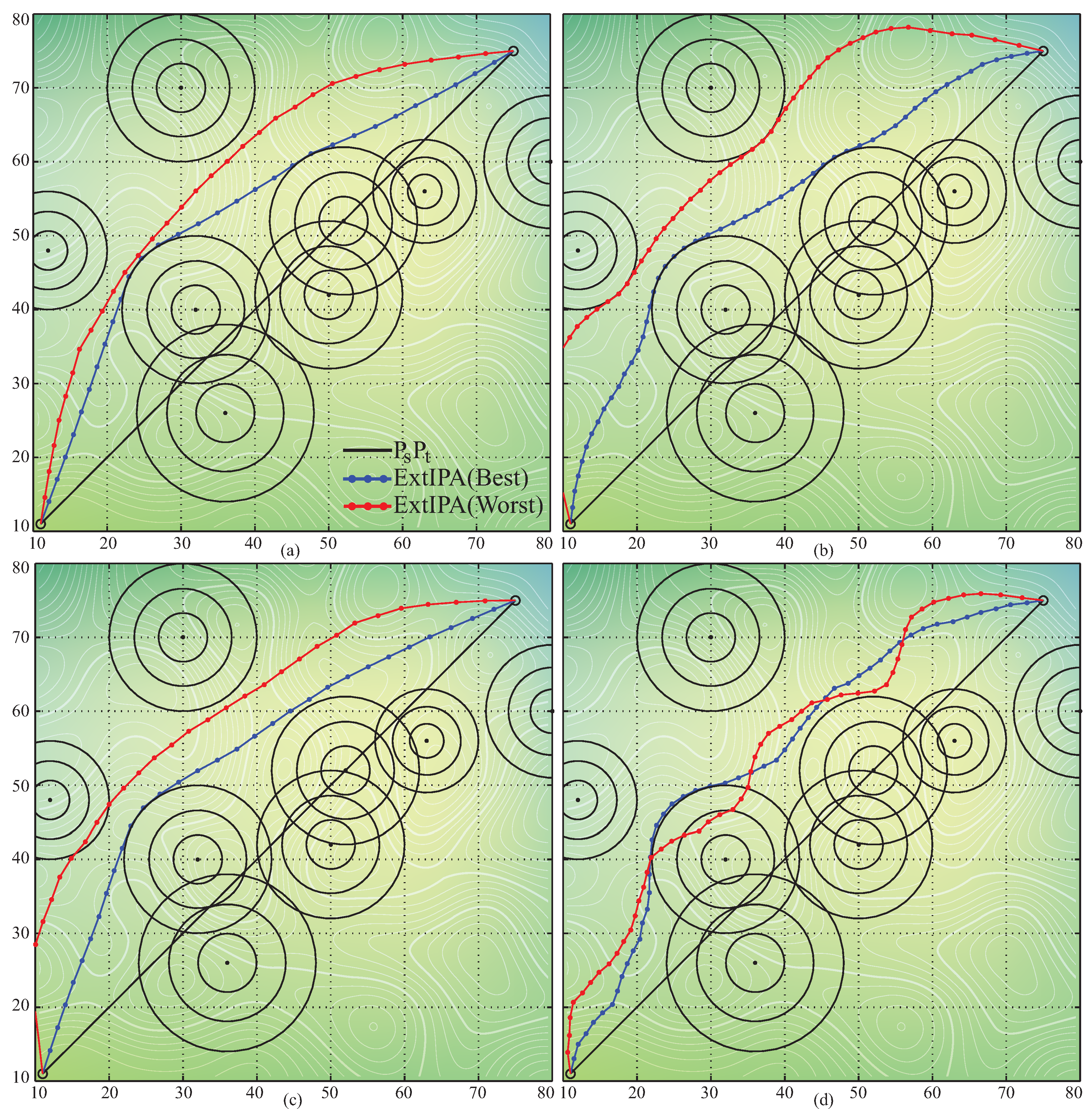
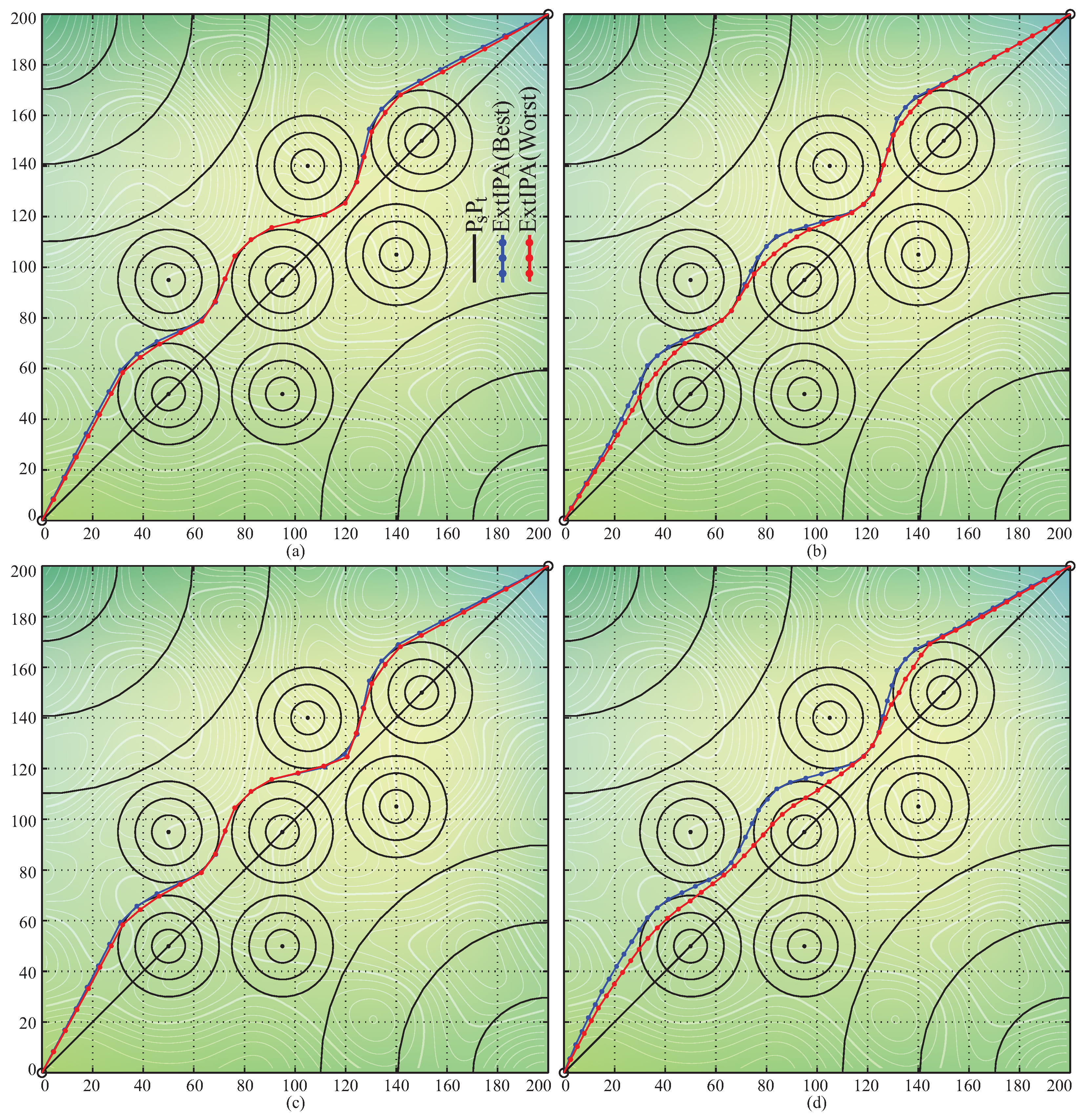
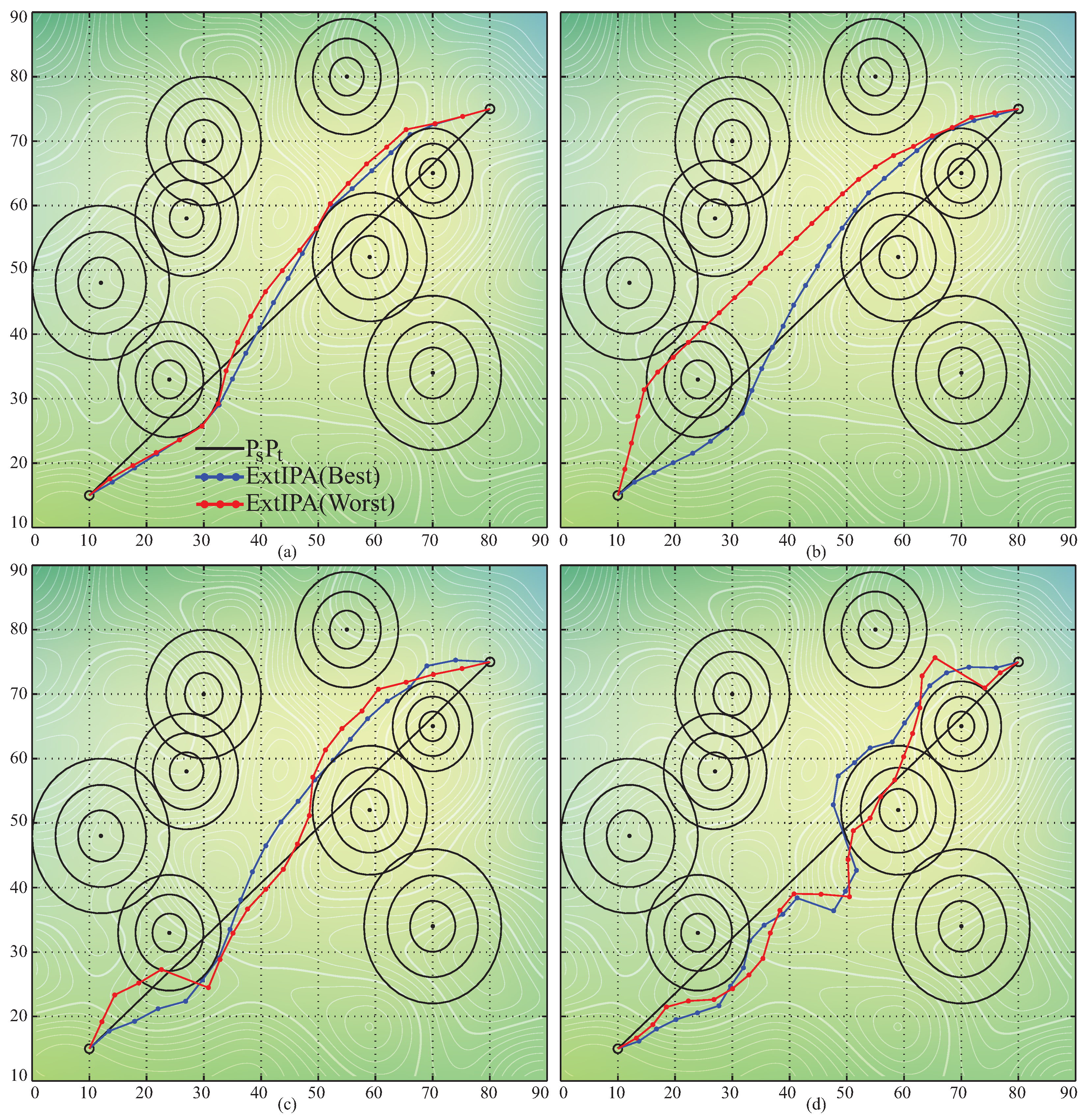
5. Experimental Studies

The qualities of the solutions calculated by a path planner can change with the properties of the considered battlefield in terms of the starting and target points, the number of enemy threats and their locations, sensing or shooting ranges, and grades. By taking into account this major requirement about the performance investigation, five challenging battlefields, detailed in

Table 1. Properties of the battlefields in the experiments.

Sc.	Threat Centers	Threat Radius	Threat Grade	Start-Target Point
1	(52, 52), (32, 40), (12, 48), (36, 26), (80, 60), (63, 56), (50, 42), (30, 70)	10, 10, 8, 12, 9, 7, 10, 10	2, 10, 1, 2, 3, 5, 2, 4	(11, 11)–(75, 75)
2	(0, 200), (200, 0), (50, 50), (95, 95), (150, 150), (95, 50), (50, 95), (140, 105), (105, 140)	90, 90, 20, 20, 20, 20, 20, 20, 20	7, 7, 5, 5 5, 6, 5, 6, 5	(0, 0)–(200, 200)
3	(59, 52), (55, 80), (27, 58), (24, 33), (12, 48), (70, 65), (70, 34), (70, 30)	10, 9, 9, 9, 12, 7, 12, 10	9, 7, 3, 12, 1, 5, 13, 2	(10, 15)–(80, 75)
4	(10, 50), (20, 20), (30, 42), (30, 80), (50, 55), (60, 10), (60, 80), (65, 38), (75, 65), (90, 80)	10, 9, 8, 10, 10, 10, 10, 12, 8, 10	8, 6, 5, 4, 7, 6, 7, 6, 8, 10	(0, 0)–(80, 100)
5	(45, 50), (12, 40), (32, 68), (36, 26), (58, 80)	10, 10, 8, 12, 9	2, 10, 1, 2, 3	(10, 10)–(55, 100)

, were used. For the first and second battlefields, the number of segmentation points and number of parameters, also abbreviated as D, were determined to be 30 and 50, while the number of segmentation points was determined to be 20 and 25 for the third battlefield and fourth battlefield, which were related with two test cases, one of which has 20 segmentation points determined optimally and the latter has 30 segmentation points. The $\lambda$ constant was set to $0.5$ with the purpose of equally weighting the cost of enemy threats and cost of fuel consumption on the J score calculation of a path [59]. In the experiments, the population size of ExtIPA was taken to be equal to 30, and five different constants, including 1, 2, 3, 4, and 5, were assigned to the $NoR$ parameter. The experiments on the first and second battlefields were repeated 50 times by setting the maximum evaluation numbers to 30,000 and 60,000, respectively [59]. Similarly, the experiments on the third and fourth battlefields were repeated 50 times by setting the maximum evaluation number to 6000 [59]. At the end of each run or test of ExtIPA, the best path found and the value of its objective function were recorded and summarized in

Table 2. Results of ExtIPA for the first four battlefields.

Sc.	D		$\mathit{NoR}$
			1	2	3	4	5
1	30	Mean	48.595	48.593	48.716	48.942	49.676
		Best	48.158	48.144	48.160	48.200	48.368
		Worst	49.771	50.245	50.562	51.697	53.322
		Std.	0.450	0.606	0.702	0.795	1.285
	50	Mean	51.167	52.057	53.198	55.562	59.367
		Best	48.600	48.694	48.829	49.875	51.629
		Worst	54.260	57.969	61.228	62.909	66.841
		Std.	1.783	2.534	3.069	3.908	4.407
2	30	Mean	152.053	153.018	152.951	153.266	153.515
		Best	149.743	149.734	149.730	149.750	150.047
		Worst	153.706	155.659	155.673	155.820	155.624
		Std.	1.347	1.659	1.666	1.844	1.486
	50	Mean	153.816	156.198	156.791	157.848	159.582
		Best	149.273	151.898	149.288	152.155	153.410
		Worst	157.542	159.238	160.430	162.613	164.025
		Std.	2.188	2.300	2.660	2.840	2.780
3	20	Mean	47.969	52.358	49.969	55.187	49.727
		Best	47.812	47.829	47.956	48.084	47.970
		Worst	48.373	58.260	63.699	63.723	58.526
		Std.	0.131	4.628	4.608	6.616	2.529
	25	Mean	50.098	57.073	50.589	53.720	56.734
		Best	48.019	47.946	48.009	48.411	48.983
		Worst	63.774	68.047	67.839	62.637	69.766
		Std.	4.079	7.450	4.478	5.190	7.432
4	20	Mean	66.397	66.570	66.596	66.664	67.480
		Best	66.363	66.345	66.370	66.335	66.942
		Worst	66.594	66.993	66.937	67.315	68.466
		Std.	0.074	0.172	0.167	0.265	0.413
	30	Mean	68.170	67.617	68.162	70.649	72.665
		Best	67.207	66.870	67.152	68.033	68.649
		Worst	70.135	68.644	70.628	83.549	82.528
		Std.	0.958	0.669	0.716	2.534	3.567

as the mean best, best, and worst objective function values and standard deviations.

The test results given in Table 2 allow us to investigate the relationship between the qualities of the calculated path, the dimensionality of the test case, and the value of the $NoR$ parameter. For six of the eight test cases, ExtIPA performs better by assigning 1 to the $NoR$ parameter when compared to the same algorithm with the remaining $NoR$ configurations. Moreover, in the 30-dimensional test cases belonging to the first and fourth battlefields, ExtIPA obtains more efficient paths with the $NoR$ configured as 2. The treatment schema of ExtIPA continues to transfer the plasma from the best individual to the receiver until the antibody level of the receiver becomes higher than the antibody level of the donor. By executing this type of treatment schema, ExtIPA consumes more evaluations on the plasma transfer operations that are responsible for maintaining the exploitation characteristics of the algorithm when ExtIPA completes the treatment of the receiver or a receivers is not determined in advance. If ExtIPA spends more evaluations on the treatment of the receiver or receivers, exploration-dominant operations related to the phase of infection distribution and the phase of the donor update cannot be sufficiently executed, and some difficulties can arise about escaping from the local optimum solution or solutions. When the $NoR$ parameter of ExtIPA is configured inappropriately for the existing population size, the qualities of the final solutions can deteriorate for some of the repetitive runs.

The population size of ExtIPA can change the performance of the algorithm like in other meta-heuristics. In order to analyze how the performance of ExtIPA varies with the different values of the $PS$ parameter, 20, 40, 50, 75, and 100 constants were used. The $NoR$ parameter of ExtIPA was set to 1 in the experiments. While 50 independent runs were carried out for the first and second battlefield scenarios after setting the maximum number of evaluations to 30,000 and 60,000, 50 independent runs were carried out for the third and fourth battlefield scenarios after setting the maximum evaluation number to 6000. The mean best, best, and worst objective function values and standard deviations given in

Table 3. Results of ExtIPA for the first four battlefields with different $PS$ values.

Sc.	D		$\mathit{PS}$
			20	30	40	50	75	100
1	30	Mean	48.526	48.595	48.835	48.606	49.223	49.472
		Best	48.160	48.158	48.185	48.181	48.197	48.206
		Worst	49.420	49.771	50.173	50.146	51.569	52.023
		Std.	0.404	0.450	0.597	0.497	1.009	1.190
	50	Mean	51.173	51.167	51.556	51.511	53.373	56.069
		Best	48.435	48.600	48.602	48.863	49.467	49.683
		Worst	53.388	54.260	56.341	56.046	57.929	63.702
		Std.	1.579	1.783	2.202	2.074	2.355	3.523
2	30	Mean	152.234	152.053	151.950	152.261	152.193	152.146
		Best	149.744	149.743	149.734	149.751	149.764	149.737
		Worst	153.747	153.706	153.720	153.834	155.036	154.023
		Std.	1.456	1.347	1.340	1.371	1.551	1.349
	50	Mean	154.318	153.816	154.440	155.328	156.165	157.016
		Best	149.298	149.273	149.544	149.656	150.530	150.619
		Worst	157.417	157.542	158.112	158.697	160.588	161.196
		Std.	1.959	2.188	1.956	2.037	2.618	2.558
3	20	Mean	50.744	47.969	48.269	50.380	52.674	55.004
		Best	47.820	47.812	48.003	48.094	48.163	48.887
		Worst	63.587	48.373	50.386	57.907	64.312	61.872
		Std.	6.070	0.131	0.452	3.548	6.082	4.588
	25	Mean	56.700	50.098	53.058	54.155	60.303	61.740
		Best	47.849	48.019	48.216	48.246	49.302	54.614
		Worst	63.880	63.774	64.016	64.329	72.984	72.348
		Std.	6.813	4.079	6.608	5.864	9.532	5.049
4	20	Mean	66.452	66.497	66.720	66.875	67.760	68.036
		Best	66.263	66.363	66.473	66.468	66.976	67.263
		Worst	66.748	66.594	66.967	67.564	69.513	69.935
		Std.	0.123	0.074	0.180	0.306	0.889	0.518
	30	Mean	67.300	68.170	68.123	69.796	72.439	78.074
		Best	66.706	67.207	67.564	68.193	68.574	71.222
		Worst	67.752	70.135	69.620	72.624	76.452	86.972
		Std.	0.352	0.958	0.525	1.241	2.710	5.664

for various $PS$ values of ExtIPA showed that the population size should be equal to or less than 40 if the dimensionality of the test cases and termination criteria are determined as detailed above. When the properties of the first four battlefields are visually inspected in Figure 2, Figure 3, Figure 4 and Figure 5, it is clearly seen that the test cases belonging to the second and third battlefields require paths containing more challenging maneuvers. When starting ExtIPA with a population in which there are some individuals partially satisfying the needed maneuvers, a relatively high population size should be chosen to increase the probability of producing the mentioned individuals or solutions. Because of this main reason, while ExtIPA with $PS$ equal to 30 or 40 finds more robust paths for the majority of the test cases related to the second and third battlefield scenarios, it should start the work with $PS$ equal to 20 or 30 for the test cases of the first and fourth battlefield scenarios.

The test cases used to evaluate the path-planning performance of ExtIPA contain at least 20 segmentation points and at most 30 segmentation points. However, the complexity of the path-planning problem can change unexpectedly with the number of segmentation points. Even though a relatively small number of segmentation points is chosen, some of the lines in the set L can intersect with the circles representing the enemy threats, and thus, selecting a point that is outside the circle or circles and on the related line becomes more difficult. Different experiments should therefore be carried out by assigning values less than 20 and more than 30 to the number of segmentation points. For this purpose, the fifth battlefield scenario containing eight cases with 5, 10, 15, 20, 25, 30, 35, and 40 segmentation points was tested. In the experiments, while the value of the $PS$ parameter of ExtIPA was set to 20, 30, 40, 50, 75, and 100, the $NoR$ parameter was taken as equal to 1. Each test case generated by combining the D and $PS$ parameters was solved 100 times by ExtIPA after setting the maximum number of evaluations to 6000 [59]. The best solution found by ExtIPA at the end of each run was recorded and then summarized in

Table 4. Results of ExtIPA for the fifth battlefield with different $PS$ values.

D		$\mathit{PS}$
		20	30	40	50	75	100
5	Mean	50.384	50.384	50.389	50.391	50.387	50.393
	Best	50.384	50.384	50.387	50.389	50.386	50.388
	Worst	50.385	50.385	50.390	50.393	50.389	50.396
	Std.	0.002	0.001	0.001	0.002	0.001	0.003
10	Mean	50.375	50.372	50.379	50.375	50.382	50.396
	Best	50.371	50.370	50.371	50.370	50.375	50.372
	Worst	50.389	50.377	50.385	50.385	50.395	50.433
	Std.	0.005	0.003	0.004	0.004	0.006	0.020
15	Mean	50.373	50.402	50.431	50.457	50.765	51.068
	Best	50.370	50.378	50.389	50.389	50.417	50.430
	Worst	50.381	50.438	50.491	50.703	51.259	52.782
	Std.	0.003	0.022	0.043	0.091	0.308	0.792
20	Mean	50.472	50.457	50.740	50.821	51.491	52.351
	Best	50.375	50.395	50.407	50.458	50.633	50.836
	Worst	50.595	50.595	51.537	52.190	53.378	54.884
	Std.	0.070	0.057	0.392	0.464	0.731	1.081
25	Mean	50.957	51.031	51.254	51.327	52.853	53.923
	Best	50.497	50.472	50.479	50.771	50.687	51.530
	Worst	53.463	52.156	53.793	52.498	54.850	57.218
	Std.	0.649	0.516	0.755	0.476	1.433	1.895
30	Mean	51.345	51.602	52.291	52.962	53.873	55.254
	Best	50.524	50.673	51.240	51.116	51.340	51.765
	Worst	52.165	53.083	53.467	56.638	56.377	62.244
	Std.	0.520	0.781	0.613	1.622	1.570	3.101
35	Mean	52.150	52.446	53.464	54.362	56.593	62.090
	Best	50.895	51.010	51.933	50.859	51.193	52.200
	Worst	54.227	55.444	59.277	58.869	62.877	68.912
	Std.	0.919	1.191	1.194	2.016	3.619	4.815
40	Mean	52.843	53.365	54.230	57.676	60.464	64.279
	Best	51.608	50.868	51.947	52.673	52.018	52.446
	Worst	55.143	55.475	56.874	61.631	71.521	81.205
	Std.	0.900	1.482	1.435	2.741	5.592	8.667

with the mean best, best, and worst objective function values and the calculated standard deviations. When the results given in Table 4 are investigated, it is clearly seen that ExtIPA performs better if the $PS$ parameter is equal to 20 or 30 for the test case of fifth battlefield. Another important conclusion that can be extracted from the results of ExtIPA for the fifth battlefield scenario is about its relatively stable performance. As stated earlier, the values being assigned to the number of segmentation points can trigger unpredictable changes in the characteristics of the path-planning problem, and an algorithm should preserve its performance for different configurations of the same battlefield. While the number of segmentation points for the fifth battlefield scenario is increased eight times from the first to the last case, the difference between the mean best objective function values is found to only be $2.459$ for the ExtIPA with 20 individuals. The best and worst paths found by ExtIPA for the fifth scenario can be seen in Figure 6.

In order to determine whether the paths planned by ExtIPA are promising or not, they should be compared with the paths found by other meta-heuristic-based path planners. For this purpose, ExtIPA was compared with the IP, ABC, I-ABC, IF-ABC, and BE-ABC algorithms for the test cases of the first and second battlefields [25,59]. To guarantee that all of the compared algorithms obtain their solutions under equal conditions, the population size and maximum evaluation number were fixed to 30 and 30,000 when solving test cases about the first battlefield scenario [25,59]. Similarly, the population size and maximum evaluation number were fixed to 30 and 60,000 when solving test cases in the second battlefield scenario [25,59]. From the test results summarized in

Table 5. Comparison between ExtIPA and other techniques for the first and second battlefields.

Sc.	D		ExtIPA	IPA	ABC	I-ABC	IF-ABC	BE-ABC
1	30	Mean	48.593	49.289	52.988	60.459	51.939	50.456
		Std.	0.606	0.465	1.425	3.288	1.343	0.672
		Rank	1	2	5	6	4	3
	50	Mean	52.057	59.354	59.972	80.174	59.956	54.982
		Std.	2.534	4.914	2.913	7.757	2.214	2.231
		Rank	1	3	5	6	4	2
2	30	Mean	152.053	151.499	154.927	185.792	153.583	153.410
		Std.	1.347	1.285	2.512	3.754	0.492	0.554
		Rank	2	1	5	6	4	3
	50	Mean	153.816	157.368	157.204	164.990	157.814	153.524
		Std.	2.188	1.596	3.603	2.811	1.905	1.047
		Rank	2	4	3	6	5	1
Average Rank			1.500	2.500	4.500	6.000	4.250	2.250
Overall Rank			1	3	5	6	4	2

after completing 50 independent runs for each algorithm, it is seen that ExtIPA has a promising performance against other competitors. While ExtIPA outperforms IPA, ABC, I-ABC, IF-ABC and BE-ABC and its rank is determined as first for the test cases in the first battlefield scenario, it lags slightly behind the IPA for the 30-dimensional case in the second battlefield, and its rank becomes second. ExtIPA lags slightly behind the BE-ABC for the 50-dimensional case in the second battlefield and its rank is found to be second. Even though the positive contribution of the extended treatment approach on the exploitation characteristics becomes more apparent in the first battlefield, some special requirements of the second battlefield concerning its exploitation limit the efficiency of the proposed method. However, it should be noticed that ExtIPA still maintains its promising performance and provides better solutions than four of its five competitors.

A path planned in the third battlefield requires challenging maneuvers similar to a safe and efficient path of the second battlefield, and a meta-heuristic-based planner should manage exploration-dominant operations more carefully. To determine whether the changes made in the workflow with the extended treatment approach allow ExtIPA to calculate more qualified paths or not, a comparison between the performances of ExtIPA, IPA, DE, PSO, BA, WDO, QPSO, QBA, and QWDO for the third battlefield was conducted. The population size of the algorithms was equal to 30 and the maximum evaluation number was set to 6000 to emphasize that they are executed under the same conditions [27,59]. When the results obtained after 50 independent runs and presented in

Table 6. Comparison between ExtIPA and other techniques for the third battlefield.

Sc.	D		ExtIPA	IPA	DE	PSO	BA	WDO	QPSO	QBA	QWDO
3	20	Mean	47.969	52.703	50.073	53.869	50.861	66.955	49.524	50.958	49.503
		Best	47.812	50.211	47.935	50.434	48.069	57.013	48.018	48.134	47.868
		Worst	48.373	55.154	51.575	59.962	52.765	74.820	51.634	56.006	50.828
		Std.	0.131	2.820	-	-	-	-	-	-	-
		Rank	1	7	4	8	5	9	3	6	2
	25	Mean	50.098	62.164	49.842	51.481	50.901	66.668	49.679	50.071	48.814
		Best	48.019	54.652	48.126	49.246	48.163	58.430	48.397	48.333	47.807
		Worst	63.774	71.302	52.110	54.246	67.441	75.967	51.307	53.423	49.749
		Std.	4.079	5.516	-	-	-	-	-	-	-
		Rank	5	8	3	7	6	9	2	4	1
Average Rank			3	7.5	3.5	7.5	5.5	9	2.5	5	1.5
Overall Rank			3	7	4	7	6	9	2	5	1

are investigated, it is seen that ExtIPA has some problems maintaining a comparative performance, especially for the 25-dimensional case in the third battlefield scenario. The initial population diversity and exploration-dominant operations of ExtIPA are generally found to be sufficient to calculate better paths compared to IPA, DE, PSO, BA, WDO, QPSO, QBA, and QWDO. However, for the 25-dimensional test case in the third battlefield scenario, because of the huge volume of the maximum evaluation number consumed by the operations related to the extended treatment approach, new solutions are not sufficiently explored, and the performance of ExtIPA deteriorates.

The comparative studies between ExtIPA and other meta-heuristic-based planners, including IPA, PSO, ABC, DE, CIJADE, JADE, and CIPDE, were continued in the fourth battlefield scenario. In these comparisons, the colony size of ABC and the population size of IPA and ExtIPA were set to 30, and the population size of PSO, DE, CIJADE, JADE, and CIPDE were set equal to 60, roughly equalizing the total number of evaluations per cycle or iteration [37]. While ABC, IPA, and ExtIPA were tested 50 times with random seeds by fixing the maximum evaluation number to 6000, PSO, DE, CIJADE, JADE, and CIPDE were tested 20 times by fixing the maximum evaluation number to 6000 [37]. The mean best, best, and worst objective function values and standard deviations calculated after completing the tests are recorded and summarized in

Table 7. Comparison between ExtIPA and other techniques for the fourth battlefield.

Sc.	D		ExtIPA	IPA	CIJADE	PSO	DE	ABC	JADE	CIPDE
4	20	Mean	66.397	68.297	66.426	70.794	67.397	67.260	66.524	66.469
		Best	66.363	67.297	66.298	67.663	66.730	66.631	66.321	66.331
		Worst	66.594	70.009	66.646	73.960	72.571	68.184	67.007	66.751
		Std.	0.074	0.682	0.087	1.869	1.249	0.512	0.193	0.126
		Rank	1	7	2	8	6	5	4	3
	30	Mean	68.170	76.496	70.297	78.982	75.197	72.656	70.407	71.033
		Best	67.207	71.334	67.622	73.753	71.766	67.845	67.521	68.170
		Worst	70.135	82.250	75.256	85.561	81.645	76.718	81.631	78.238
		Std.	0.958	2.823	1.813	3.828	2.434	2.147	3.026	2.502
		Rank	1	7	2	8	6	5	3	4
Average Rank			1	7	2	8	6	5	3.500	3.500
Overall Rank			1	7	2	8	6	5	3	3

. As seen from the results given in Table 7, ExtIPA produces more robust and efficient paths compared to the other tested algorithms. The promising performance of the ExtIPA can already be seen for the 30- and 50-dimensional cases in the first and second battlefields, and 20-dimensional case in the third battlefield was also validated for the 20- and 30-dimensional cases in the fourth battlefield. A detailed search within the vicinity of a qualified solution, as is performed in the extended treatment, helps the algorithm to subtly calibrate the selected points from the lines and thus plan more satisfactory UCAV paths. Because of the presence of enemy threats and their locations, effect ranges, and grades in the fourth battlefield decrease the probability of generating eligible paths using dense exploration-based operations, ExtIPA gets a chance to show its robust and stable convergence performance more apparently in the mean best objective function values and standard deviations.

The performance validation of ExtIPA was concluded after a comparison with other meta-heuristic algorithms, including IPA, ABC, BA, ACO, BBO, DE, ES, FA, GA, PBIL, and PSO and some of their variants, such as BAM, MFA, SGA, and PGSO, in the fifth battlefield scenario. The path planners used for the test cases of the fifth battlefield were run 100 times by setting the population size to 30 and the maximum evaluation number to 6000 [21,57]. The mean best, best, and worst objective function values and related standard deviations of them calculated after 100 independent runs are given in

Table 8. Comparison between ExtIPA and other techniques for the fifth battlefield.

Sc.	D		ExtIPA	IPA	ABC	BA	BAM	ACO	BBO	DE	ES	FA	GA	MFA	PBIL	PSO	SGA	PGSO
5	5	Mean	50.384	50.384	50.384	106.483	59.054	61.520	72.730	58.596	80.720	58.750	60.470	59.167	66.139	59.906	60.501	53.669
		Best	50.384	50.384	50.384	60.690	54.357	61.372	60.330	54.357	59.590	54.359	55.247	54.357	59.763	55.167	55.654	53.380
		Worst	50.385	50.385	50.385	345.255	60.240	63.320	171.500	62.200	112.260	65.740	61.600	62.419	72.250	66.071	61.200	60.630
		Std.	0.001	0.001	0.001	-	-	-	-	2.160	-	3.010	-	2.250	-	2.620	1.560	2.260
		Rank	1	1	1	16	7	12	14	5	15	6	10	8	13	9	11	4
	10	Mean	50.372	50.398	50.384	69.425	52.707	61.950	57.965	53.104	76.280	52.180	52.542	51.574	101.440	57.041	52.279	50.849
		Best	50.370	50.376	50.371	52.360	51.395	60.228	52.947	51.395	57.420	51.399	51.607	51.397	83.112	52.207	51.549	50.649
		Worst	50.377	50.457	50.406	108.738	60.7244	68.190	76.820	56.736	123.460	56.710	60.110	53.786	119.250	68.622	56.165	53.330
		Std.	0.003	0.024	0.013	-	-	-	-	2.600	-	2.370	-	1.730	-	2.250	1.430	1.870
		Rank	1	3	2	14	9	13	12	10	15	6	8	5	16	11	7	4
	15	Mean	50.402	50.570	50.591	63.601	51.231	60.260	59.526	52.278	71.860	52.822	52.188	50.897	128.250	58.340	51.891	51.516
		Best	50.378	50.424	50.425	53.075	50.609	58.530	52.557	50.611	58.255	50.617	50.871	50.612	107.223	52.097	50.807	50.452
		Worst	50.438	51.219	50.789	85.745	60.192	61.000	90.370	62.580	103.860	94.276	57.447	53.832	189.200	87.320	61.800	55.460
		Std.	0.022	0.193	0.100	-	-	-	-	3.730	-	4.250	-	1.340	-	4.010	2.450	1.490
		Rank	1	2	3	14	5	13	12	9	15	10	8	4	16	11	7	6
	20	Mean	50.457	50.925	52.181	63.630	50.760	66.220	61.88	52.722	70.190	53.733	53.090	50.700	185.430	58.248	53.167	52.398
		Best	50.395	50.495	50.866	52.395	50.467	60.445	54.723	50.510	60.232	50.463	50.825	50.455	130.152	52.464	50.846	50.657
		Worst	50.595	51.271	54.672	83.706	53.742	67.180	78.200	64.570	81.450	78.914	59.180	52.028	337.300	78.160	68.950	59.850
		Std.	0.057	0.196	0.994	-	-	-	-	3.710	-	7.580	-	1.020	-	6.950	3.990	1.560
		Rank	1	4	5	13	2	14	12	7	15	10	8	2	16	11	9	6
	25	Mean	51.031	51.678	54.690	64.901	50.709	61.570	64.780	54.408	72.780	53.904	53.781	50.999	257.720	60.263	54.157	54.587
		Best	50.472	50.790	51.911	55.017	50.448	61.549	55.528	50.551	63.369	50.491	51.242	50.457	159.740	53.738	51.239	50.782
		Worst	52.156	57.314	57.530	74.926	53.519	62.070	80.330	69.660	83.910	66.452	60.398	53.704	699.600	78.139	65.700	63.160
		Std.	0.516	1.503	1.618	-	-	-	-	4.120	-	8.660	-	0.810	-	7.550	4.060	2.380
		Rank	3	4	10	14	1	12	13	8	15	6	5	2	16	11	7	9
	30	Mean	51.602	51.789	59.805	66.616	51.106	63.950	67.870	59.988	74.780	54.962	55.008	51.357	395.540	62.385	54.521	56.891
		Best	50.673	50.997	54.527	57.247	50.467	63.230	56.607	50.898	65.725	50.683	51.921	50.516	230.150	53.299	51.617	51.019
		Worst	53.083	61.565	64.940	80.084	60.285	64.710	78.580	74.120	91.300	65.976	62.718	58.336	2396	93.695	64.710	75.320
		Std.	0.781	2.275	2.366	-	-	-	-	6.740	-	9.120	-	1.230	-	8.200	4.110	3.450
		Rank	3	4	9	13	1	12	14	10	15	6	7	2	16	11	5	8
	35	Mean	52.446	55.889	66.187	67.703	51.461	68.310	71.560	67.900	76.520	55.996	55.960	51.601	684.660	64.135	55.826	59.744
		Best	51.010	51.005	57.259	57.448	50.479	66.960	63.021	52.537	66.745	51.083	52.311	50.471	270.330	55.503	51.633	54.136
		Worst	55.444	96.301	74.095	82.737	58.819	68.720	93.850	84.440	88.76	83.887	74.479	55.883	6362	82.833	67.610	71.450
		Std.	1.191	12.249	4.298	-	-	-	-	9.150	-	9.550	-	1.650	-	8.650	4.120	4.010
		Rank	3	5	10	11	1	13	14	12	15	7	6	2	16	9	4	8
	40	Mean	53.365	55.994	75.595	69.973	51.876	74.580	74.850	77.620	80.260	57.856	57.493	52.198	1169	64.885	57.110	62.420
		Best	50.868	51.025	63.269	58.650	50.602	69.795	63.550	54.549	68.231	51.523	52.208	50.561	390.620	55.737	52.618	55.092
		Worst	55.475	116.195	86.613	83.263	58.427	77.060	90.700	93.260	96.420	86.663	72.069	57.724	7103	84.730	67.870	72.650
		Std.	1.482	16.188	5.356	-	-	-	-	10.900	-	10.430	-	2.380	-	9.410	4.550	4.540
		Rank	3	4	13	10	1	11	12	14	15	7	6	2	16	9	5	8
Average Rank			2.000	3.375	6.625	13.125	3.375	12.500	12.875	9.375	15.000	7.250	7.250	3.375	15.625	10.250	6.875	6.625
Overall Rank			1	2	5	14	2	12	13	10	15	8	8	2	16	11	7	5

. One of the important results extracted from this table is the superiority of the ExtIPA over all of fifteen competitors for the 5-, 10-, 15-, and 20-dimensional cases in the existing battlefield scenario. On the other hand, when the remaining test cases in the fifth battlefield are considered, it is seen that ExtIPA lags behind both BAM and MFA and becomes the third best path planner. As stated previously, the number of segmentation points can completely change the properties of the optimal path being planned for a UAV or UCAV, even if the same battlefield is considered. Each extra segmentation point can cause problems related to the escaping enemy threats and increasing total flight length, and handling these special requirements for all test cases of a battlefield, such as the fifth battlefield, can be challenging. Because of this situation, while ExtIPA dominates other algorithms for some test cases and is ranked as the best planner among them, other problem instances become more suitable to the search characteristics of the BAM and MFA path planners for the 25-, 30-, 35-, and 40-dimensional cases in the fifth battlefield. However, it should be still considered that ExtIPA is able to preserve its path-planning capability compared to BAM and MFA when all eight cases are evaluated together, and its average and overall ranks and smaller standard deviations prove the strong and stable performance of the algorithm.

The paths and their objective function values found by different path planners are relatively close to each other for most cases of the fifth battlefield scenario. Even though the average and overall ranks provide information which algorithm is capable of dominating other competitors, an appropriate test should also be employed for investigating whether the superiority of the considered algorithm can be validated statistically or not. Wilcoxon signed rank test is one of the most commonly used tests for deciding there is a statistical difference in favor of one of the compared techniques. If the significance level abbreviated as $\rho$ with Wilcoxon signed rank test is less than a constant that is usually determined as $0.05$, it is said that one of the algorithm is statistically better than another [60]. In order to understand that ExtIPA is statistically better than other path planners for the fifth battlefield scenario or not, Wilcoxon signed rank test with the significance level $0.05$ was executed by considering the mean best, best and worst objective function values and its results were presented in

Table 9. Statistical comparison between ExtIPA and other planners for the fifth scenario using the mean best objective function values.

ExtIPA vs.	IPA	ABC	BA	BAM	ACO
Z-val.	2.417	2.417	2.660	0.197	2.660
$\rho$-val.	0.015	0.015	0.007	0.843	0.007
$W+$	0	0	0	16	0
$W-$	28	28	36	20	36
Sign.	ExtIPA	ExtIPA	ExtIPA	-	ExtIPA
ExtIPA vs.	BBO	DE	ES	FA	GA
Z-val.	2.660	2.660	2.660	2.660	2.660
$\rho$-val.	0.007	0.007	0.007	0.007	0.007
$W+$	0	0	0	0	0
$W-$	36	36	36	36	36
Sign.	ExtIPA	ExtIPA	ExtIPA	ExtIPA	ExtIPA
ExtIPA vs.	MFA	PBIL	PSO	SGA	PGSO
Z-val.	0.328	2.660	2.660	2.660	2.660
$\rho$-val.	0.742	0.007	0.007	0.007	0.007
$W+$	15	0	0	0	0
$W-$	21	36	36	36	36
Sign.	-	ExtIPA	ExtIPA	ExtIPA	ExtIPA

,

Table 10. Statistical comparison between ExtIPA and other planners for the fifth scenario using the best objective function values.

ExtIPA vs.	IPA	ABC	BA	BAM	ACO
Z-val.	2.153	2.417	2.660	0.328	2.660
$\rho$-val.	0.031	0.015	0.007	0.742	0.007
$W+$	1	0	0	15	0
$W-$	27	28	36	21	36
Sign.	ExtIPA	ExtIPA	ExtIPA	-	ExtIPA
ExtIPA vs.	BBO	DE	ES	FA	GA
Z-val.	2.660	2.660	2.660	2.660	2.660
$\rho$-val.	0.007	0.007	0.007	0.007	0.007
$W+$	0	0	0	0	0
$W-$	36	36	36	36	36
Sign.	ExtIPA	ExtIPA	ExtIPA	ExtIPA	ExtIPA
ExtIPA vs.	MFA	PBIL	PSO	SGA	PGSO
Z-val.	0.328	2.660	2.660	2.660	2.660
$\rho$-val.	0.742	0.007	0.007	0.007	0.007
$W+$	15	0	0	0	0
$W-$	21	36	36	36	36
Sign.	-	ExtIPA	ExtIPA	ExtIPA	ExtIPA

and

Table 11. Statistical comparison between ExtIPA and other planners for the fifth scenario using the worst objective function values.

ExtIPA vs.	IPA	ABC	BA	BAM	ACO
Z-val.	2.153	2.417	2.660	0.328	2.660
$\rho$-val.	0.031	0.015	0.007	0.742	0.007
$W+$	1	0	0	15	0
$W-$	27	28	36	21	36
Sign.	ExtIPA	ExtIPA	ExtIPA	-	ExtIPA
ExtIPA vs.	BBO	DE	ES	FA	GA
Z-val.	2.660	2.660	2.660	2.660	2.660
$\rho$-val.	0.007	0.007	0.007	0.007	0.007
$W+$	0	0	0	0	0
$W-$	36	36	36	36	36
Sign.	ExtIPA	ExtIPA	ExtIPA	ExtIPA	ExtIPA
ExtIPA vs.	MFA	PBIL	PSO	SGA	PGSO
Z-val.	0.328	2.660	2.660	2.660	2.660
p-val.	0.742	0.007	0.007	0.007	0.007
$W+$	15	0	0	0	0
$W-$	21	36	36	36	36
Sign.	-	ExtIPA	ExtIPA	ExtIPA	ExtIPA

. In these tables, Z value shows the test statistics. While the $W+$ abbreviation represents the sum of ranks for which ExtIPA is worse than other planner, the $W-$ abbreviation represents the sum of ranks for which ExtIPA is better than other planner. From the test results given in Table 9, Table 10 and Table 11, it is seen that while the performance of ExtIPA is statistically better than the IPA, ABC, BA, ACO, BBO, DE, ES, FA, GA, PBIL, PSO, SGA and PGSO with $\rho$ values less than 0.05, the significance is not in favor of ExtIPA for the comparison between ExtIPA and BAM or MFA.

The extended treatment approach can accelerate the convergence speed. Because the treatment of a receiver is continued until the antibody level of the receiver becomes higher than the antibody level of its donor, the extended treatment can boost the convergence to the global optimum. However, it should be noticed that if the treatment takes longer, different stagnation periods can be seen on the convergence curves. To evaluate the convergence performances of the algorithms, the success rate ($Sr$) and mean evaluations ($Me$) are two commonly used metrics [60]. If an algorithm obtains a solution whose objective function value is better than the previously determined threshold, it is assumed that the algorithm is successful for the considered run and the percentage of the number of successful runs to the total number of runs corresponds to the $Sr$. When a run is labeled as successful, the minimum number of evaluations required to find a solution with an objective function value better than threshold is recorded. The average of the recorded values is also matched with the $Me$ metric. From the $Sr$ and $Me$ metrics calculated by setting the threshold as 55, as given in

Table 12. $Sr$ and $Me$ values of ExtIPA, IPA, and ABC for the fifth scenario.

D		ExtIPA	IPA	ABC
5	$Sr$	100.000	100.000	100.000
	$Me$	103.920	217.454	210.474
10	$Sr$	100.000	100.000	100.000
	$Me$	308.170	1324.990	850.474
15	$Sr$	100.000	100.000	100.000
	$Me$	782.190	2049.330	2037.113
20	$Sr$	100.000	100.000	100.000
	$Me$	1244.450	2609.247	3946.557
25	$Sr$	100.000	98.990	61.856
	$Me$	1885.310	3889.194	5435.733
30	$Sr$	100.000	98.990	5.155
	$Me$	2887.850	3904.888	5923.000
35	$Sr$	95.000	86.000	0.000
	$Me$	3465.211	4305.440	-
40	$Sr$	90.000	90.000	0.000
	$Me$	4147.200	4380.840	-

for the fifth battlefield, it is understood that the convergence performance of ExtIPA is more robust than the convergence performances of both the IPA- and ABC-based planners. For the first four test cases related to the considered battlefield scenario, ExtIPA, IPA, and ABC are capable of obtaining better solutions with objective function values less than the threshold in each of the 100 independent runs. However, it should be noticed that ExtIPA requires at least two times fewer evaluations compared to IPA and ABC for the 5-, 10-, 15-, and 20-dimensional test cases. When the dimensionality of the test cases is increased starting from 25 to 40, while ExtIPA and IPA still preserve their convergence characteristics, ABC has some difficulties reaching the given threshold, and no successful run is detected for the cases with 35 and 40 segmentation points.

6. Conclusions

Recent years have witnessed dramatic paradigm and strategic changes in the military and commercial operations carried out by UAVs and their customized variants carrying complex optical, targeting, and weapon systems called UCAVs. To improve the success of a task being employed with one of these advanced aerial vehicles, a flight path should be carefully determined by taking into account some challenging optimization objectives that must be satisfied about the enemy air defense systems, fuel or battery usage, or total cruise length. The immune plasma algorithm (IP algorithm or IPA) is one of the most recent nature-inspired computational intelligence techniques, and its promising performance has been validated on different numerical benchmarks and engineering problems. In this study, the plasma transfer schema of the IPA was completely changed with a newly introduced extended treatment approach, and the extended IP algorithm (ExtIPA) was proposed as a UAV or UCAV path planner. To investigate the path-planning capabilities of ExtIPA, five different battlefield scenarios and various algorithm-specific parameter configurations were used.

The paths found by the ExtIPA were also compared with the paths found by well-known meta-heuristic algorithms such as ABC, BA, ACO, BBO, DE, ES, FA, GA, PSO, PBIL, and WDO and some of their improved versions, such as BAM, MFA, SGA, PGSO, I-ABC, IF-ABC, BE-ABC, QPSO, QBA, QWDO, CIJADE, JADE, and CIPDE. Comparative studies between ExtIPA and other path planners showed that the extended treatment approach contributes to the efficiency of plasma transfer operations by ensuring the treatment will be continued until a poor solution, represented by a receiver individual becoming better than its donor, and ExtIPA outperforms the other algorithms in most of the test cases. Moreover, ExtIPA removed the necessity of using the $NoD$ parameter and resolved some difficulties around guessing the interaction between $NoD$ and $NoR$ and then assigning appropriate values to them to obtain better solutions. In the future, ExtIPA can be further improved by integrating a mechanism that adjusts the $NoR$ parameter adaptively. The IP algorithm with multiple populations each executing a unique treatment procedure can be designed and used to solve UAV or UCAV path-planning problems made difficult by the existence of dynamic obstacles, enemy threats, and real-time calculations.

References

1. Tisdale, J.; Kim, Z.; Hedrick, J.K. Autonomous UAV path planning and estimation. IEEE Robot. Autom. Mag. 2009, 16, 35–42. [Google Scholar] [CrossRef]
2. Hermand, E.; Nguyen, T.W.; Hosseinzadeh, M.; Garone, E. Constrained control of UAVs in geofencing applications. In Proceedings of the 2018 26th Mediterranean Conference on Control and Automation (MED), Zadar, Croatia, 19–22 June 2018; pp. 217–222. [Google Scholar] [CrossRef]
3. Chen, J.; Zhang, R.; Zhao, H.; Li, J.; He, J. Path planning of multiple unmanned aerial vehicles covering multiple regions based on minimum consumption ratio. Aerospace 2023, 10, 93. [Google Scholar] [CrossRef]
4. Song, J.; Zhao, K.; Liu, Y. Survey on mission planning of multiple unmanned aerial vehicles. Aerospace 2023, 10, 208. [Google Scholar] [CrossRef]
5. Ait Saadi, A.; Soukane, A.; Meraihi, Y.; Benmessaoud Gabis, A.; Mirjalili, S.; Ramdane-Cherif, A. UAV path planning using optimization approaches: A survey. Arch. Comput. Methods Eng. 2022, 29, 4233–4284. [Google Scholar] [CrossRef]
6. Bal, M. An overview of path planning technologies for unmanned aerial vehicles. Therm. Sci. 2022, 26, 2865–2876. [Google Scholar] [CrossRef]
7. Wu, Y. A survey on population-based meta-heuristic algorithms for motion planning of aircraft. Swarm Evol. Comput. 2021, 62, 100844. [Google Scholar] [CrossRef]
8. Majeed, A.; Hwang, S.O. A multi-objective coverage path planning algorithm for UAVs to cover spatially distributed regions in urban environments. Aerospace 2021, 8, 343. [Google Scholar] [CrossRef]
9. Saeed, R.A.; Omri, M.; Abdel-Khalek, S.; Ali, E.S.; Alotaibi, M.F. Optimal path planning for drones based on swarm intelligence algorithm. Neural Comput. Appl. 2022, 34, 10133–10155. [Google Scholar] [CrossRef]
10. Xu, C.; Duan, H.; Liu, F. Chaotic artificial bee colony approach to Uninhabited Combat Air Vehicle (UCAV) path planning. Aerosp. Sci. Technol. 2010, 14, 535–541. [Google Scholar] [CrossRef]
11. Zhang, Y.; Wu, L.; Wang, S. UCAV path planning based on FSCABC. Inf.-Int. Interdiscip. J. 2011, 14, 687–692. [Google Scholar]
12. Zhang, Y.; Wu, L.; Wang, S. UCAV path planning by fitness-scaling adaptive chaotic particle swarm optimization. Math. Probl. Eng. 2013, 2013. [Google Scholar] [CrossRef]
13. Li, P.; Duan, H. Path planning of unmanned aerial vehicle based on improved gravitational search algorithm. Sci. China Technol. Sci. 2012, 55, 2712–2719. [Google Scholar] [CrossRef]
14. Fu, Z.F. Path planning of UCAV based on a modified GeesePSO algorithm. In Proceedings of the International Conference on Intelligent Computing, Huangshan, China, 25–29 July 2012; pp. 471–478. [Google Scholar] [CrossRef]
15. Wang, G.G.; Guo, L.; Duan, H.; Liu, L.; Wang, H. A modified firefly algorithm for UCAV path planning. Int. J. Hybrid Inf. Technol. 2012, 5, 123–144. [Google Scholar]
16. Wang, G.G.; Guo, L.; Duan, H.; Wang, H.; Liu, L.; Shao, M. A hybrid metaheuristic DE/CS algorithm for UCAV three-dimension path planning. Sci. World J. 2012, 2012, 583973. [Google Scholar] [CrossRef] [PubMed]
17. Wang, G.G.; Guo, L.; Duan, H.; Liu, L.; Wang, H. A bat algorithm with mutation for UCAV path planning. Sci. World J. 2012, 2012, 418946. [Google Scholar] [CrossRef]
18. Wang, G.G.; Chu, H.E.; Mirjalili, S. Three-dimensional path planning for UCAV using an improved bat algorithm. Aerosp. Sci. Technol. 2016, 49, 231–238. [Google Scholar] [CrossRef]
19. Zhu, W.; Duan, H. Chaotic predator–prey biogeography-based optimization approach for UCAV path planning. Aerosp. Sci. Technol. 2014, 32, 153–161. [Google Scholar] [CrossRef]
20. Heidari, A.; Abbaspour, R. Improved black hole algorithm for efficient low observable UCAV path planning in constrained aerospace. Adv. Comput. Sci. Int. J. 2014, 3, 87–92. [Google Scholar]
21. Tang, Z.; Zhou, Y. A glowworm swarm optimization algorithm for uninhabited combat air vehicle path planning. J. Intell. Syst. 2015, 24, 69–83. [Google Scholar] [CrossRef]
22. Yu, G.; Song, H.; Gao, J. Unmanned aerial vehicle path planning based on TLBO algorithm. Int. J. Smart Sens. Intell. Syst. 2014, 7, 1310–1325. [Google Scholar] [CrossRef]
23. Zhang, X.; Duan, H. An improved constrained differential evolution algorithm for unmanned aerial vehicle global route planning. Appl. Soft Comput. 2015, 26, 270–284. [Google Scholar] [CrossRef]
24. Zhou, Q.; Zhou, Y.; Chen, X. A wolf colony search algorithm based on the complex method for uninhabited combat air vehicle path planning. Int. J. Hybrid Inf. Technol. 2014, 7, 183–200. [Google Scholar] [CrossRef]
25. Li, B.; Gong, L.G.; Yang, W.L. An improved artificial bee colony algorithm based on balance-evolution strategy for unmanned combat aerial vehicle path planning. Sci. World J. 2014, 2014, 232704. [Google Scholar] [CrossRef] [PubMed]
26. Zhang, B.; Duan, H. Three-dimensional path planning for uninhabited combat aerial vehicle based on predator-prey pigeon-inspired optimization in dynamic environment. IEEE/ACM Trans. Comput. Biol. Bioinform. 2015, 14, 97–107. [Google Scholar] [CrossRef]
27. Zhou, Y.; Bao, Z.; Wang, R.; Qiao, S.; Zhou, Y. Quantum wind driven optimization for unmanned combat air vehicle path planning. Appl. Sci. 2015, 5, 1457–1483. [Google Scholar] [CrossRef]
28. Zhang, S.; Zhou, Y.; Li, Z.; Pan, W. Grey wolf optimizer for unmanned combat aerial vehicle path planning. Adv. Eng. Softw. 2016, 99, 121–136. [Google Scholar] [CrossRef]
29. Luo, Q.; Li, L.; Zhou, Y. A quantum encoding bat algorithm for uninhabited combat aerial vehicle path planning. Int. J. Innov. Comput. Appl. 2017, 8, 182–193. [Google Scholar] [CrossRef]
30. Zhang, Q.; Wang, R.; Yang, J.; Ding, K.; Li, Y.; Hu, J. Modified collective decision optimization algorithm with application in trajectory planning of UAV. Appl. Intell. 2018, 48, 2328–2354. [Google Scholar] [CrossRef]
31. Alihodzic, A.; Tuba, E.; Capor-Hrosik, R.; Dolicanin, E.; Tuba, M. Unmanned aerial vehicle path planning problem by adjusted elephant herding optimization. In Proceedings of the 2017 25th Telecommunication Forum (Telfor), Belgrade, Serbia, 21–22 November 2017; pp. 1–4. [Google Scholar] [CrossRef]
32. Alihodzic, A.; Hasic, D.; Selmanovic, E. An effective guided fireworks algorithm for solving UCAV path planning problem. In Proceedings of the International Conference on Numerical Methods and Applications, Borovets, Bulgaria, 20–24 August 2018; pp. 29–38. [Google Scholar] [CrossRef]
33. Miao, F.; Zhou, Y.; Luo, Q. A modified symbiotic organisms search algorithm for unmanned combat aerial vehicle route planning problem. J. Oper. Res. Soc. 2019, 70, 21–52. [Google Scholar] [CrossRef]
34. Dolicanin, E.; Fetahovic, I.; Tuba, E.; Capor-Hrosik, R.; Tuba, M. Unmanned combat aerial vehicle path planning by brain storm optimization algorithm. Stud. Inform. Control 2018, 27, 15–24. [Google Scholar] [CrossRef]
35. Pan, J.S.; Liu, J.L.; Hsiung, S.C. Chaotic cuckoo search algorithm for solving unmanned combat aerial vehicle path planning problems. In Proceedings of the 2019 11th International Conference on Machine Learning and Computing, Zhuhai, China, 22–24 February 2019; pp. 224–230. [Google Scholar] [CrossRef]
36. Pan, J.S.; Liu, J.L.; Liu, E.J. Improved whale optimization algorithm and its application to UCAV path planning problem. In Proceedings of the International Conference on Genetic and Evolutionary Computing, Qingdao, China, 1–3 November 2019; pp. 37–47. [Google Scholar] [CrossRef]
37. Pan, J.S.; Liu, N.; Chu, S.C. A hybrid differential evolution algorithm and its application in unmanned combat aerial vehicle path planning. IEEE Access 2020, 8, 17691–17712. [Google Scholar] [CrossRef]
38. Lin, N.; Tang, J.; Li, X.; Zhao, L. A novel improved bat algorithm in UAV path planning. J. Comput. Mater. Contin. 2019, 61, 323–344. [Google Scholar] [CrossRef]
39. Qu, C.; Gai, W.; Zhong, M.; Zhang, J. A novel reinforcement learning based grey wolf optimizer algorithm for unmanned aerial vehicles (UAVs) path planning. Appl. Soft Comput. 2020, 89, 106099. [Google Scholar] [CrossRef]
40. Qu, C.; Gai, W.; Zhang, J.; Zhong, M. A novel hybrid grey wolf optimizer algorithm for unmanned aerial vehicle (UAV) path planning. Knowl.-Based Syst. 2020, 194, 105530. [Google Scholar] [CrossRef]
41. Yi, J.H.; Lu, M.; Zhao, X.J. Quantum inspired monarch butterfly optimisation for UCAV path planning navigation problem. Int. J.-Bio-Inspired Comput. 2020, 15, 75–89. [Google Scholar] [CrossRef]
42. Wu, C.; Huang, X.; Luo, Y.; Leng, S. An improved fast convergent artificial bee colony algorithm for unmanned aerial vehicle path planning in battlefield environment. In Proceedings of the 2020 IEEE 16th International Conference on Control & Automation (ICCA), Sapporo, Japan, 6–9 July 2020; pp. 360–365. [Google Scholar] [CrossRef]
43. Chen, Y.; Pi, D.; Xu, Y. Neighborhood global learning based flower pollination algorithm and its application to unmanned aerial vehicle path planning. Expert Syst. Appl. 2021, 170, 114505. [Google Scholar] [CrossRef]
44. Zhu, H.; Wang, Y.; Ma, Z.; Li, X. A comparative study of swarm intelligence algorithms for ucav path-planning problems. Mathematics 2021, 9, 171. [Google Scholar] [CrossRef]
45. Zhu, H.; Wang, Y.; Li, X. UCAV path planning for avoiding obstacles using cooperative co-evolution spider monkey optimization. Knowl.-Based Syst. 2022, 246, 108713. [Google Scholar] [CrossRef]
46. Zhou, X.; Gao, F.; Fang, X.; Lan, Z. Improved bat algorithm for UAV path planning in three-dimensional space. IEEE Access 2021, 9, 20100–20116. [Google Scholar] [CrossRef]
47. Wu, P.; Li, T.; Song, G. UCAV path planning based on improved chaotic particle swarm optimization. In Proceedings of the 2020 Chinese Automation Congress (CAC), Shanghai, China, 6–8 November 2020; pp. 1069–1073. [Google Scholar] [CrossRef]
48. Xu, H.; Jiang, S.; Zhang, A. Path planning for unmanned aerial vehicle using amix-strategy-based gravitational search algorithm. IEEE Access 2021, 9, 57033–57045. [Google Scholar] [CrossRef]
49. Jiang, W.; Lyu, Y.; Li, Y.; Guo, Y.; Zhang, W. UAV path planning and collision avoidance in 3D environments based on POMPD and improved grey wolf optimizer. Aerosp. Sci. Technol. 2022, 121, 107314. [Google Scholar] [CrossRef]
50. Wang, X.; Pan, J.S.; Yang, Q.; Kong, L.; Snášel, V.; Chu, S.C. Modified mayfly algorithm for UAV path planning. Drones 2022, 6, 134. [Google Scholar] [CrossRef]
51. Niu, Y.; Yan, X.; Wang, Y.; Niu, Y. An adaptive neighborhood-based search enhanced artificial ecosystem optimizer for UCAV path planning. Expert Syst. Appl. 2022, 208, 118047. [Google Scholar] [CrossRef]
52. Jia, Y.; Qu, L.; Li, X. A double-layer coding model with a rotation-based particle swarm algorithm for unmanned combat aerial vehicle path planning. Eng. Appl. Artif. Intell. 2022, 116, 105410. [Google Scholar] [CrossRef]
53. Aslan, S.; Demirci, S. Immune plasma algorithm: A novel meta-heuristic for optimization problems. IEEE Access 2020, 8, 220227–220245. [Google Scholar] [CrossRef]
54. Kisa, M.; Demirci, S.; Arslan, S.; Aslan, S. Solving channel assignment problem in cognitive radio networks with immune plasma algorithm. In Proceedings of the 2021 6th International Conference on Computer Science and Engineering (UBMK), Ankara, Turkey, 15–17 September 2021; pp. 818–822. [Google Scholar] [CrossRef]
55. Arslan, S. Solving the problem of time series prediction using immune plasma programming. Avrupa Bilim Teknol. Derg. 2022, 219–224. [Google Scholar] [CrossRef]
56. Tasdemir, A.; Demirci, S.; Aslan, S. Performance investigation of immune plasma algorithm on solving wireless sensor deployment problem. In Proceedings of the 2022 9th International Conference on Electrical and Electronics Engineering (ICEEE), Alanya, Turkey, 29–31 March 2022; pp. 296–300. [Google Scholar] [CrossRef]
57. Aslan, S.; Demirci, S. An improved immune plasma algorithm with a regional pandemic restriction. Signal Image Video Process. 2022, 16, 2093–2101. [Google Scholar] [CrossRef]
58. Ajay, V.; Nesasudha, M. Detection of attackers in cognitive radio network using optimized neural networks. Intell. Autom. Soft Comput. 2022, 34, 193–204. [Google Scholar] [CrossRef]
59. Aslan, S.; Erkin, T. An immune plasma algorithm based approach for UCAV path planning. J. King Saud-Univ.-Comput. Inf. Sci. 2023, 35, 56–69. [Google Scholar] [CrossRef]
60. Aslan, S.; Karaboga, D.; Badem, H. A new artificial bee colony algorithm employing intelligent forager forwarding strategies. Appl. Soft Comput. 2020, 96, 106656. [Google Scholar] [CrossRef]
Figure 1. Initial (a) and transformed (b) coordinate systems, calculated paths (c), and their counterparts for the initial coordinate system (d).
Aerospace 10 00487 g001
Figure 2. The best and worst paths of ExtIPA with  P S  equal to 30 for 30-dimensional (a) and 50-dimensional (b) cases of the first scenario and with  P S  equal to 100 for 30-dimensional (c) and 50-dimensional (d) cases of the first scenario.
Aerospace 10 00487 g002
Figure 3. The best and worst paths of ExtIPA with  P S  equal to 30 for 30-dimensional (a) and 50-dimensional (b) cases of the second scenario and with  P S  equal to 100 for 30-dimensional (c) and 50-dimensional (d) cases of the second scenario.
Aerospace 10 00487 g003
Figure 4. The best and worst paths of ExtIPA with  P S  equal to 30 for 20-dimensional (a) and 25-dimensional (b) cases of the third scenario and with  P S  equal to 100 for 20-dimensional (c) and 25-dimensional (d) cases of the third scenario.
Aerospace 10 00487 g004
Figure 5. The best and worst paths of ExtIPA with  P S  equal to 30 for 20-dimensional (a) and 30-dimensional (b) cases of the fourth scenario and with  P S  equal to 100 for 20-dimensional (c) and 30-dimensional (d) cases of the fourth scenario.
Aerospace 10 00487 g005
Figure 6. The best and worst paths of ExtIPA with  P S  equal to 30 for 25-dimensional (a) and 40-dimensional (b) cases of the fifth scenario and with  P S  equal to 100 for 25-dimensional (c) and 40-dimensional (d) cases of the fifth scenario.
Aerospace 10 00487 g006