1. Introduction
During the transonic flight of a vehicle, the phenomenon of self-excited shock oscillation caused by shock wave-boundary layer interaction at a certain combination of Mach numbers and angle of attack is called transonic buffet. This phenomenon involves unsteady flows, and there is still a lack of a unified explanation for its mechanism. Early researchers explained the occurrence mechanism of transonic buffet by constructing a feedback model of shock–Kutta wave interaction [
1]. In addition, Crouch et al. [
2,
3]. drew the conclusion that such instability could lead to shock oscillations and dramatic lift fluctuations from the perspective of the global instability of the flow. Despite the possibility of encountering buffet, transonic flight has higher flight efficiency, therefore, most modern high-speed aircraft still use transonic speed as the cruise flight state. However, the pulsating load caused by transonic buffet can cause aircraft control deterioration, structural fatigue, and even flight accidents. The research on transonic buffet of vehicles has been difficult and has therefore become a hot spot in the field of aviation.
The early suppression and the elimination of the adverse effects of transonic buffet are usually conducted by two methods: control [
4,
5,
6,
7] and aerodynamic shape optimization [
8]. Control is further divided into active control and passive control. There are two common passive control methods: (1) from the structural point of view, increasing structural damping to suppress transonic buffet or installing vibration isolators to protect the internal instruments of the vehicle; (2) changing the flow characteristics of the fluid on the wing surface, such as trailing edge slotting. The streamwise slot is a simple passive control [
4,
5] that can retard the expansion of flow separation caused by normal shock, but it is not effective in controlling the shock of periodic self-excited oscillations. The active control method is mainly to suppress the transonic buffet by improving the flow stability, such as installing a fluidic vortex generator (FVG) and a trailing edge deflector (TED) to control the flow in the trailing edge region. Yun [
9] designed a shock control bump with a specific shape to achieve effective control of buffet. Gao et al. [
10] established an unsteady flow model with oscillatory shock and a moving boundary. The model-based feedback control of buffet by trailing edge flap was designed by using pole configuration and the linear quadratic method respectively, which effectively controls the buffet. The open-loop, closed-loop, and machine learning adaptive control for buffet was also realized.
Although control measures are effective in controlling buffet, they often require additional structure and weight. In contrast, the aerodynamic shape optimization method can consider the transonic buffet constraint from the perspective of airfoil design, which can effectively achieve buffet suppression and also expand the flight envelope at the design stage. In addition, this method is carried out at the early stage of the vehicle design, which can reduce the design cost. Therefore, the aerodynamic shape optimization design is an ideal approach for the suppression of transonic buffet of a vehicle.
Thanks to the rapid development of computer technology, the accuracy and efficiency of CFD technology have been significantly improved. With the efficient CFD technology and optimization algorithm, the efficiency of aerodynamic shape optimization design has been greatly improved. It has gradually become a hot spot for research in various disciplines. At present, the aerodynamic shape optimization can be roughly divided into three categories according to different optimization methods: gradient optimization; global optimization based on the surrogate model; aerodynamic shape optimization based on machine learning.
Gradient optimization refers to identification of the optimal point by finding the partial derivatives of the objective function with respect to the design variables to determine the search direction. The gradient of the objective function can be derived by the direct method or the adjoint equation method [
11]. Compared with the direct method, the efficiency of the adjoint method depends only on the number of objective functions, which validates its computational advantages. Jameson [
12] first proposed the adjoint method based on Euler’s equation for transonic aerodynamic shape optimization of a vehicle. In terms of unsteady aerodynamic optimization, Nadarajah and Jameson [
13] used this method to perform unsteady aerodynamic optimization of a helicopter rotor with drag reduction as the optimization objective, and achieved a 46% reduction in drag. Lee et al. [
14] carried out flapping airfoils optimization based on the unsteady discrete adjoint approach. Although the adjoint gradient-based optimization method has fast convergence and high optimization efficiency, it is a local optimization algorithm, and the optimization falls into a local optimum. The global optimization algorithm can find the global optimal solution. However, in the process of aerodynamic shape optimization, the number of CFD calls of the global optimization algorithm is much larger than that of the gradient optimization algorithm, which also requires high computational cost. In order to improve the optimization efficiency, it is meaningful to use mathematical means to replace the large number of CFD numerical calculations in the optimization process by surrogate models. Sun [
15] established a surrogate model based on artificial neural network to realize the optimization of aircraft aerodynamic performance. Wu [
16] used a non-intrusive polynomial method and Kriging model to construct a stochastic surrogate model with random aerodynamic characteristics, and adaptively updated it based on historical optimization data to carry out optimization design. The model dimensionality is reduced based on the idea of transformation and decomposition. Later, with the booming development of machine learning, in order to further improve the efficiency of optimization, researchers began to apply it to aerodynamic shape optimization design. Li [
17] used the data-driven approach to optimize the aerodynamic shape for buffet-onset constraint. Hu [
18] used an artificial intelligence method based on deep neural networks to improve efficiency. In addition, Viquerat et al. [
19]. used deep reinforcement learning to perform direct shape optimization and applied it to the field of aerodynamics, that is, the optimal design of the aerodynamic shape of a vehicle. Runze [
20] used a deep reinforcement learning approach based on a surrogate model to achieve the optimal design of drag reduction for a supercritical airfoil in a steady state. Therefore, the introduction of machine learning made the optimization framework more efficient.
Most of the previous aerodynamic shape optimizations were performance optimizations in a steady state, where a surrogate model between lift-drag and shape parameters was constructed by CFD. In contrast, transonic buffet optimization involves an unsteady flow problem where it is difficult to build a traditional surrogate model. The reinforcement learning derived from machine learning, has a powerful inductive learning capability, and has great potential for application in the field of flow field modeling and aerodynamic optimization [
21,
22,
23,
24].
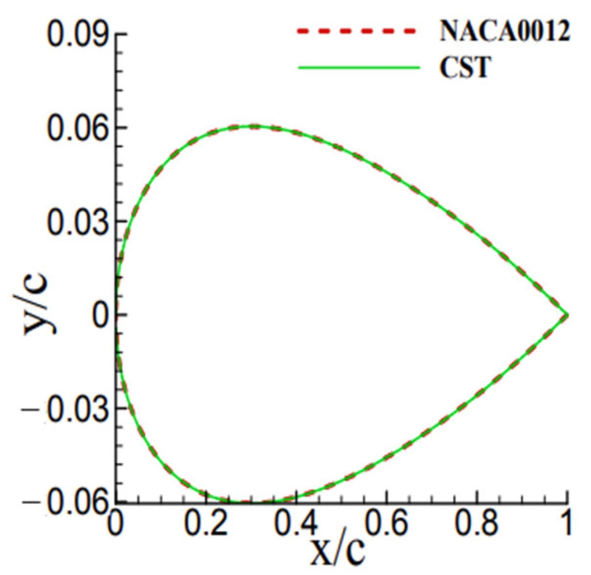
This paper studies from the perspective of aerodynamic shape optimization, which is able to obtain the desired aerodynamic performance by adjusting the aerodynamic shape of a vehicle (e.g., airfoil) without adding additional structures or devices. Based on reinforcement learning, a framework is constructed for the aerodynamic shape optimization design of a vehicle using the deep deterministic policy gradient (DDPG) algorithm. The class shape transformation parametric method is performed to represent the airfoil shape efficiently and accurately with a small number of parameters. The aerodynamic performance is calculated by CFD approach based on the Reynolds average Navier–Stokes. Using this framework, it is possible to achieve the optimal design of the aerodynamic shape of a vehicle in an unsteady state.
3. Reinforcement Learning-Based Design Framework for Aerodynamic Optimization
3.1. DDPG Algorithm
Reinforcement learning can be categorized into two types at the model level: model-based and model-free. In the model-based approach, an agent learns a model that describes how the environment works based on its observations and uses this model to plan actions. However, in most applications, the model is unknown. A way to find the optimal policy without modeling the environment is model-free reinforcement learning. The DDPG is a model-free approach to reinforcement learning, which is a mathematical model that does not rely on the environment, usually with actions as inputs and states as outputs. The DDPG algorithm [
30] contains several networks and related concepts, the mathematical definitions of which are given below.
Deterministic action policy
: in the DDPG algorithm, the action
of the agent at each step is calculated by Equation (6), where
denotes the state:
Actor network : the deterministic action policy is approximated by applying a fully connected neural network, and the approximated network is called the actor network. The actor network consists of two parts: the online actor network and the target actor network. The online actor network updates the network parameters and selects an action based on the current state , which is used to interact with the environment and generate the next state and reward . The target actor network selects the optimal next action based on the next state .
Action policy distribution : this is the distribution function of the set of states produced by an agent under a certain action policy .
Value function: this is the value expectation obtained by taking action
under state
according to deterministic action policy
, based on the definition of Bellman equation as shown in Equation (7):
Critic network: as can be seen from Equation (7), the value function is a recursive function, and in order to avoid recursively computing the value , the DDPG algorithm approximates the value function using a fully connected neural network, which is named the critic network .
In the DDPG algorithm, the actor network
is used to represent the deterministic policy
in reinforcement learning, and the input and output are the state
and the deterministic action
. The critic network
is used to represent the action value function
, and is used to solve the Bellman equation. The actor network is used to update the policy and the critic network is used to approximate the value function. The objective function is the expectation of discounted cumulative rewards, as shown in the following equation:
The optimal deterministic policy
is the policy that maximizes the objective function
:
The gradient of the objective function
with respect to the actor network
is equivalent to the expected gradient of
with respect to
. Therefore, the derivative of
can be derived based on the chain derivative rule. The method for updating the actor network is obtained as shown in Equation (9):
In the above equation,
denotes the reward
obtained after choosing an action according to policy
in state
. And
. With the deterministic policy
, Equation (9) can be deformed as
The objective function which uses the gradient ascent algorithm in Equation (9) above is optimally designed. To reach the goal of increasing the cumulative reward expectation, the agent is made to update the actor network along the direction of increasing .
The critic network in the DDPG algorithm, on the other hand, is updated based on the deep Q-learning (DQN) approach [
31], and the critic network gradient is shown as follows:
where the target
value is
and
denote the target critic network and the target actor network, respectively. The goal of the DDPG algorithm training is to maximize the target function
while minimizing the loss of the critic network
. Similarly, the critic network is divided into the online critic network and the target critic network. The former updates the network parameters and calculates the Q-value of the current state-action pair
; while the latter is responsible for calculating the
.
3.2. Reinforcement Learning-Based Optimization Framework
The framework of reinforcement learning contains five elements: agent, state, environment, reward, and action. Among them, the agent is the ontology of reinforcement learning and acts as the decision maker or learner in the process. The environment refers to everything in the reinforcement learning except the agent, which mainly consists of the state set. In this framework, the environment refers to the flow field. The state is loaded with the data of the environment. The action refers to the action made by the agent. After making an action, the agent obtains the reward signal from the environment and learns how to maximize this reward.
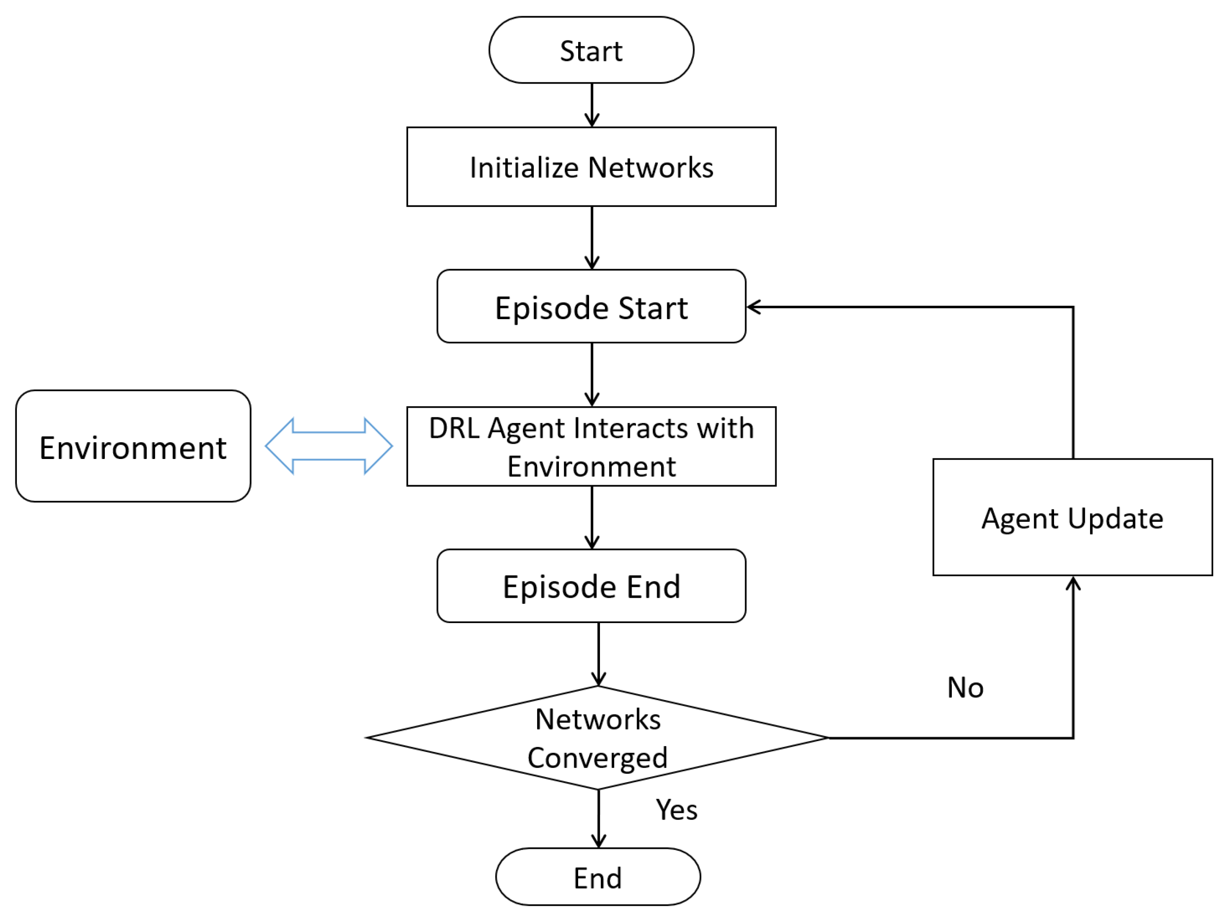
Figure 4 shows the block diagram of the reinforcement learning process, where the algorithm first initializes the grid parameters and then interacts with the environment. During each interaction, the agent outputs an action based on the state observed from the environment, after which the environment moves to the next state and provides feedback on the reward. The agent judges whether the network parameters converge at the end of each round; if they do not, they are optimized using the interaction data; and if they do, the reinforcement learning optimization is ended.
In this paper, the reinforcement learning framework is divided into the following modules: (1) empirical cache pool; (2) fully connected neural network framework; (3) reinforcement learning algorithm; (4) main function. The empirical cache pool realizes the data caching and sampling extraction of the interaction between the flow field (environment) and the optimization system. The fully-connected neural network framework module implements the fully-connected neural network framework construction. Set the activation function. The reinforcement learning algorithm module inherits the above two modules and sets up the optimizer to realize sampling from the experience cache pool. It then calculates the difference between the output of the actor and critic networks and the target value, and optimizes the two groups of networks and the saving and loading of the network model. The relevant hyperparameters are set in the main function, and the flow simulation executable is called. After one round, the data is read into the experience cache pool, and the loss function is defined according to the optimization target. The neural network is optimized, and the optimization process reward changes are recorded, while the neural network parameters are saved after the convergence condition is satisfied. The actor network has three layers; the input is the state and the output is the action; the intermediate layer has an input dimension. The critic network also has three layers; the input is the state and action, and the output is the reward; the middle layer input dimension is 256, while the output dimension is 128.
3.3. Optimization Framework Validation
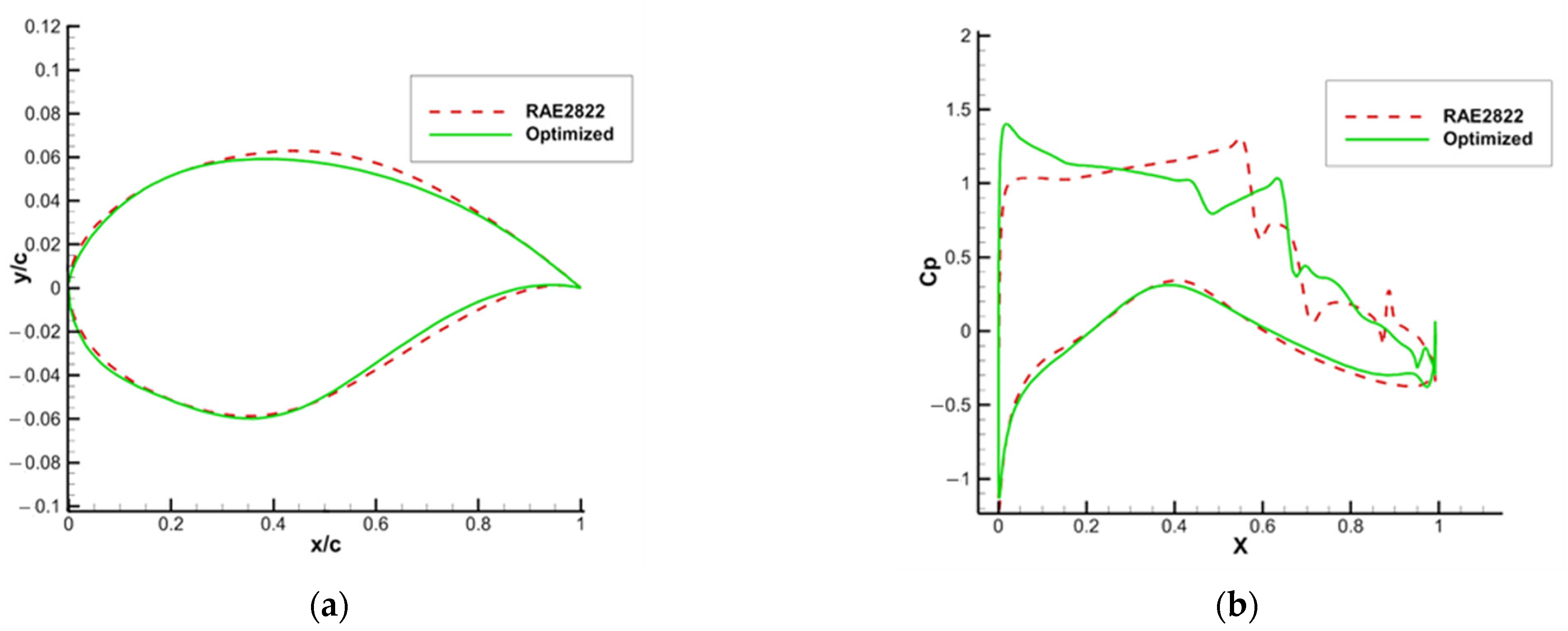
The proposed optimization framework in airfoil optimization is verified through a comparative study. The airfoil steady drag reduction optimization is performed for the RAE2822 airfoil using the reinforcement learning-based aerodynamic shape optimization framework, with reference to the study on aerodynamic shape optimization conducted by Wu et al. [
16,
32].
In the study of Wu et al. [
32], the optimized design of drag reduction airfoil for the RAE2822 airfoil was carried out in steady state, and the optimized state was selected as Ma = 0.734, Re = 6.5 × 10
6, α = 2.8°. The optimized mathematical model is shown in Equation (10):
The lift coefficient, airfoil area and pitch moment coefficient constraints with drag coefficient reduction are set as the goal. The optimization state is consistent with that in the reference, and the optimization results in this section are given in
Table 1 for comparison with the results of Wu et al. [
32]. Compared with the airfoil drag reduction rate of 42% of the reference, the optimized framework achieves a stronger one of about 46% from 0.0193 to 0.0105.
Figure 5a shows the results of optimization; (b) shows the pressure coefficient distribution on the airfoil surface before and after the optimization.
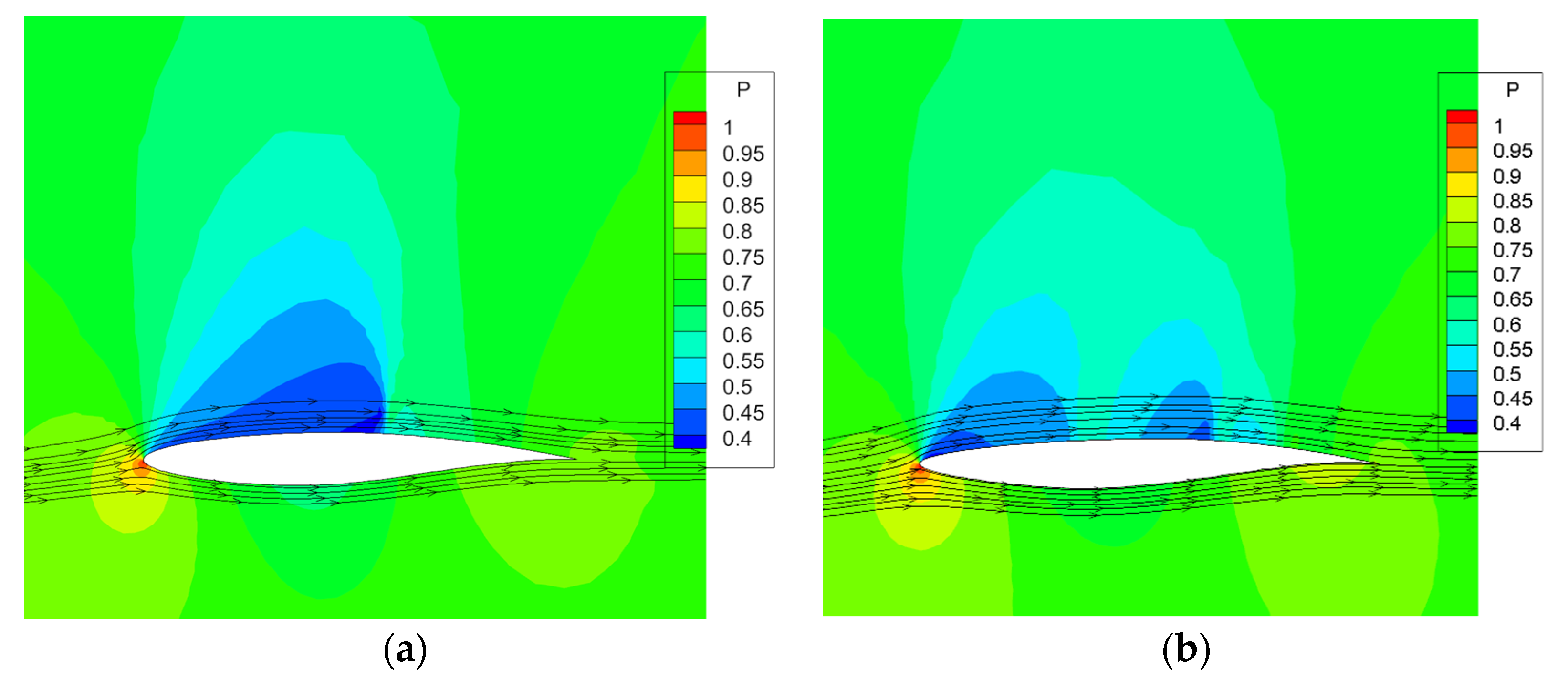
Figure 6 shows the comparison of flow field before and after the drag reduction optimization. After optimization, the airfoil shock intensity is significantly weakened, and the distribution of pressure coefficients on the upper surface is similar to the literature results [
32], with two shocks, the first of which is close to the leading edge position of the airfoil, and the drag force is reduced.
4. Reinforcement Learning-Based Optimization for Transonic Buffet
The variance of the lift coefficient is chosen as the buffet optimization design index. The transonic buffet of the aircraft involves the unsteady flow of the fluid, and the determination of the design index is the prerequisite for buffet optimization. Successfully characterizing the strength of the buffet and refining the optimization index determine the success of the optimization. Thomas and Dowell et al. [
33]. used the amplitude of lift coefficient pulsation generated by the airfoil as the optimization objective, and its practical effect is to achieve buffet suppression by suppressing the lift pulsation under forced motion. In addition, Kenway and Martins [
34] used the separation zone on the wing surface as an indicator to assess the buffet strength. However, since buffet occurs in an unsteady state, this makes the area of the separation very difficult to solve, coupled with the increase in the angle of attack, while the gradual expansion of the separation zone contradicts the existence of exit boundary of the buffet. Xu et al. [
35] used the buffet load as a design index and constructed a surrogate model to carry out the optimal design of the aerodynamic shape of the vehicle. In this work, the following points were considered.
- (1)
By considering the airfoil as a stationary rigid body, the original problem is simplified to optimize the elimination of the pulsation load generated by the flow instability on the airfoil surface.
- (2)
Since the pulsation of the lift coefficient is often the strongest among all the aerodynamic indices when the flow instability buffet occurs, the goal of the optimized design is to suppress it.
- (3)
The design index is extracted from the indicators characterizing the strength of the lift coefficient pulsation, while the variance of the lift coefficient within a certain period of time is selected as the design index.
- (4)
Optimization is carried out in the state of strong lift pulsation, and different design states are selected for different airfoil types.
- (5)
The research on aerodynamic shape optimization design is based on reinforcement learning.
The constructed mathematical model for transonic buffet optimization is given by Equation (11).
is the variance of the lift coefficient, which is used to characterize the buffet strength, and
;
is the number of sampling points of the lift coefficient;
and
denote the mean values of lift coefficient and drag coefficient, respectively;
is the maximum thickness of the airfoil:
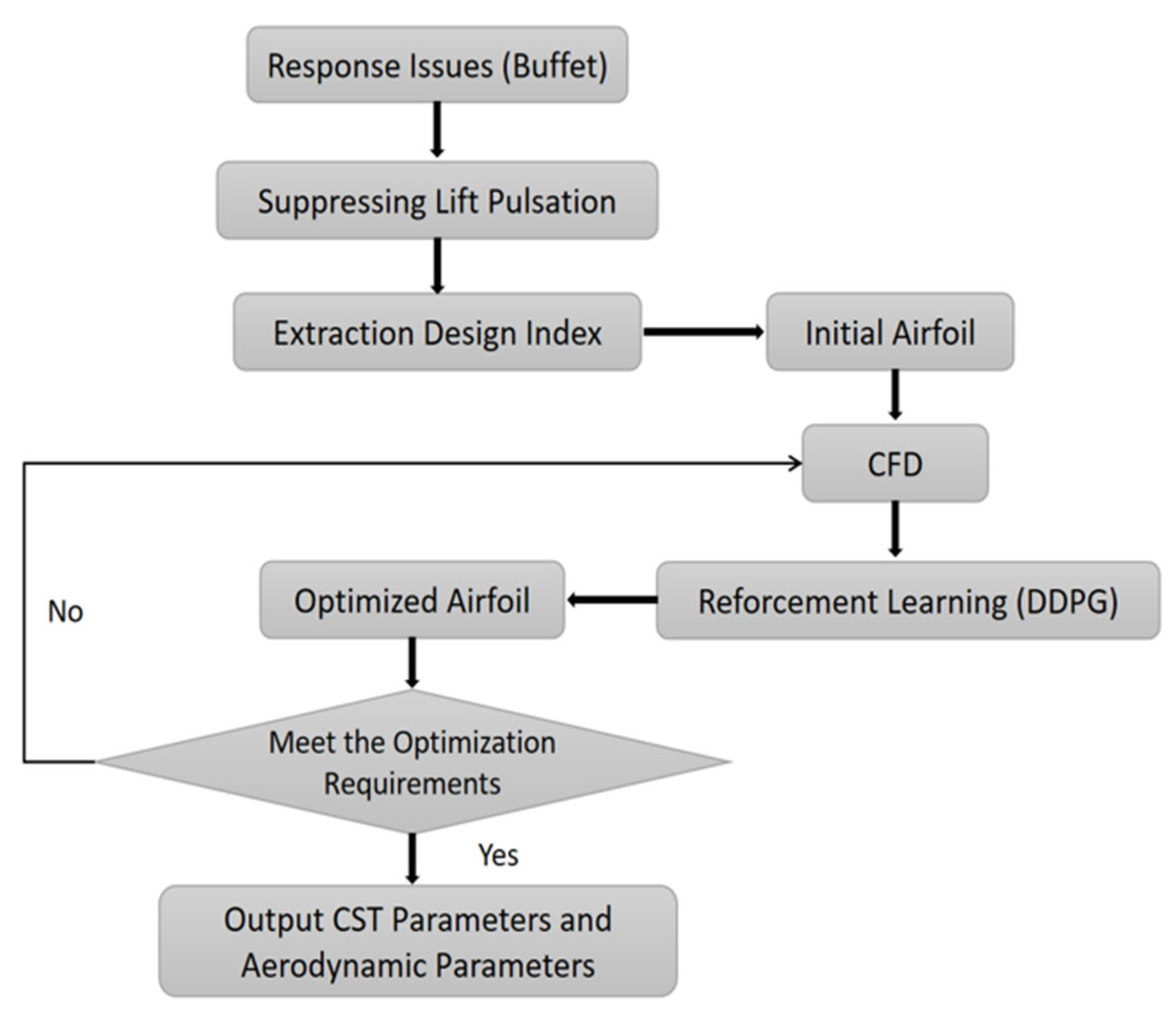
Figure 7 shows the research framework of the reinforcement learning-based transonic buffet optimization design.
4.1. NACA0012 Airfoil Buffet Optimization
The reinforcement learning reward is set according to Equation (11). For the base airfoil NACA0012, the state Ma = 0.7, α = 5.5°, and Re = 3 × 10
6 has intense transonic buffet, and so it is selected as the optimized state. The reinforcement learning reward is set as follows:
is the variance of lift coefficient, which is the target, to ensure that the optimized airfoil can play a significant role in suppressing buffet. is the difference between the time-averaged values of the lift coefficients before and after optimization, which is one of the constraints to guarantee that the lift performance of the optimized airfoil. In addition, is the drag constraint to ensure that the drag performance of the optimized airfoil will not deteriorate. is the maximum thickness of the airfoil, and its geometry shape is constrained by setting this objective. ω is the weighting factor of the objective and each constraint. denote the time-averaged values of the lift coefficient and drag coefficient of the initial airfoil NACA0012, respectively, and is the maximum thickness of the airfoil NACA0012.
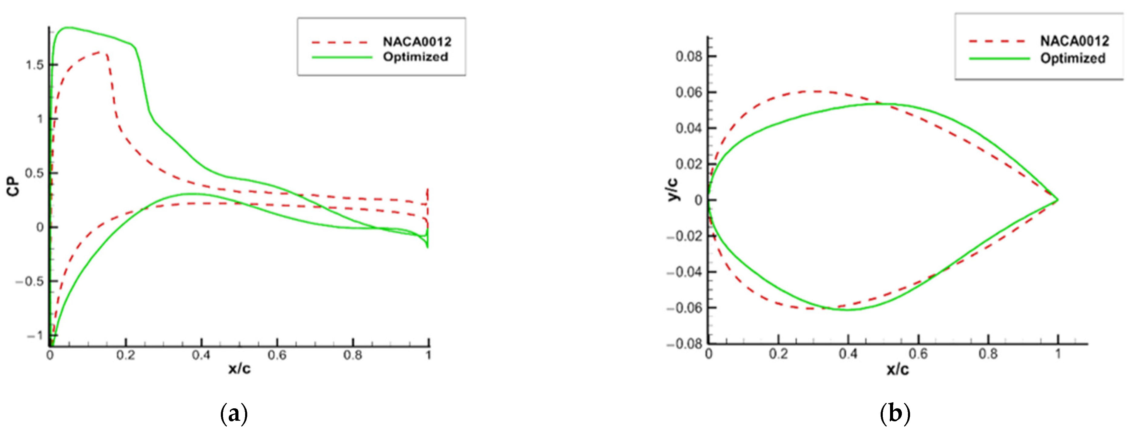
As shown in
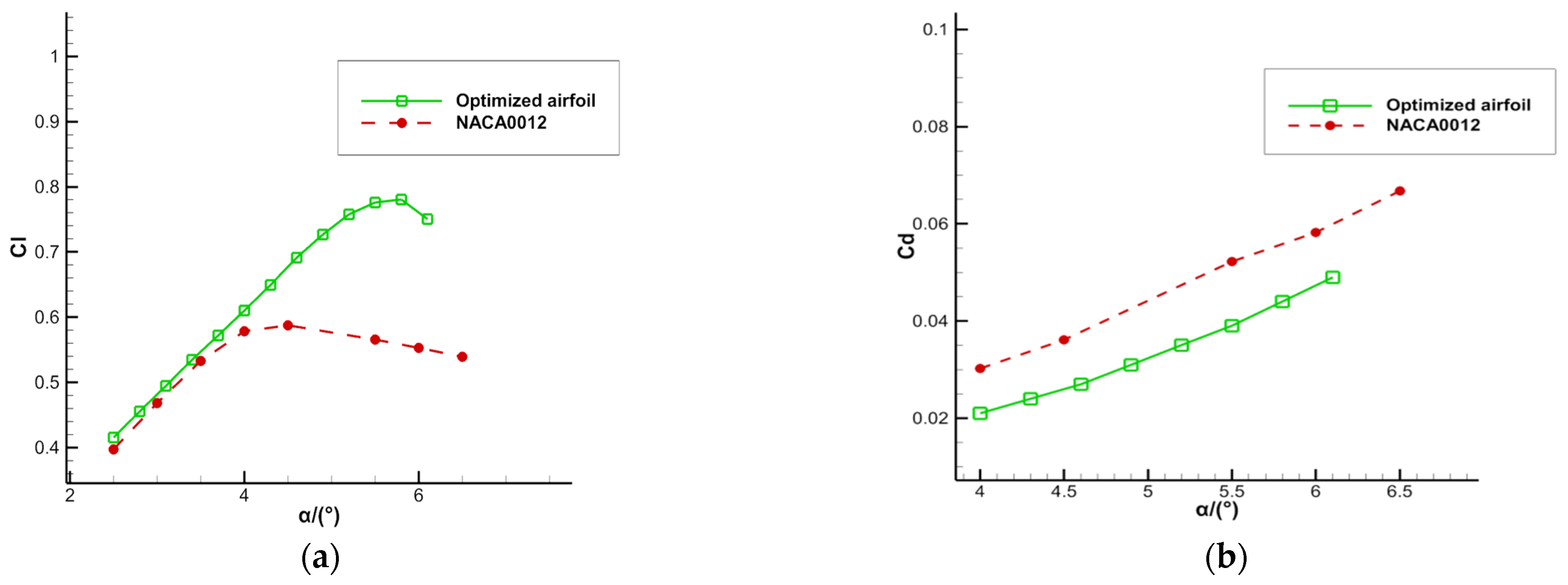
Figure 8, while the leading edge of the optimized airfoil is obviously narrower, the maximum thickness position is shifted back from 0.3 times of the original chord length to about 0.4 times of that. However, the maximum thickness remains meanwhile unchanged, the thickness of the trailing edge is slightly increased, and the leading edge of the airfoil narrows. As shown in
Figure 9, the optimized airfoil has a higher lift coefficient and lower drag coefficient, which improves the aerodynamic performance compared to the initial airfoil. As shown in
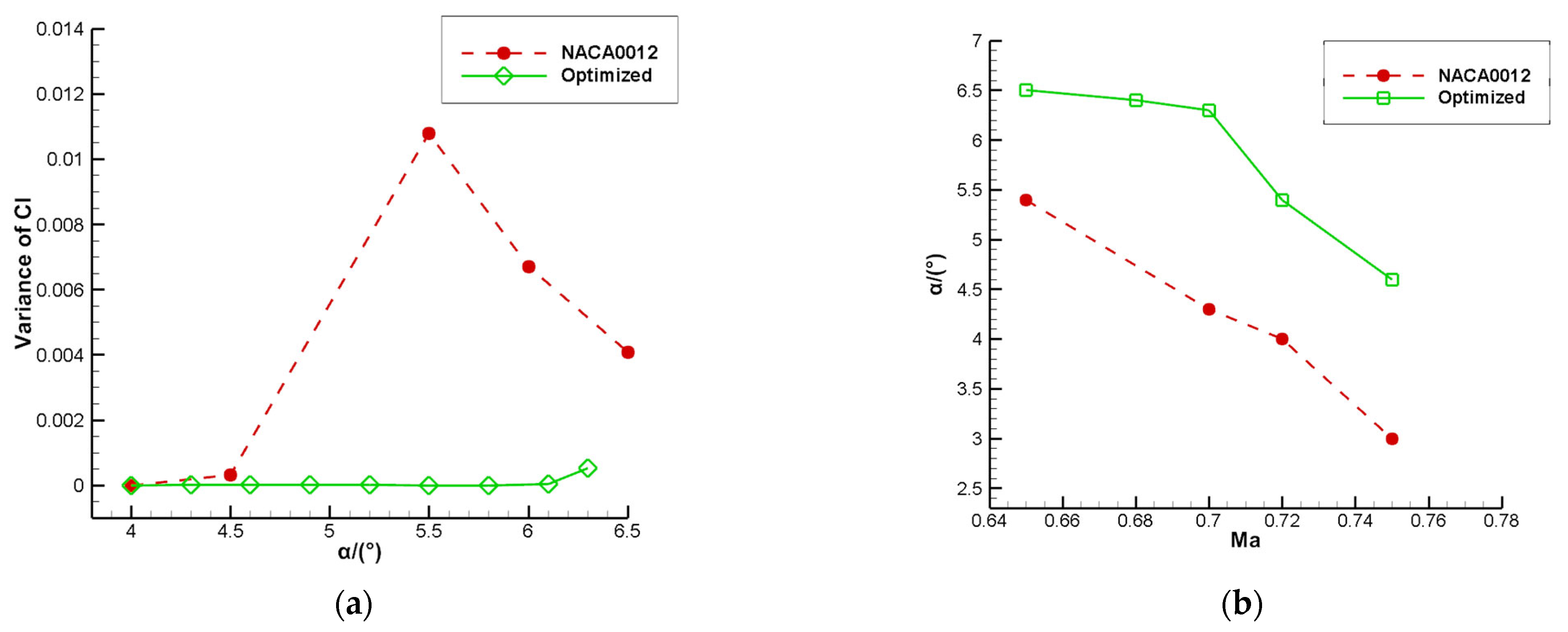
Figure 10, the buffet is completely suppressed in the optimized state and the buffet onset boundary is raised. No buffet occurs between 4° and 6.1°, and only a slight buffet occurs at 6.3°.
Figure 10b shows the comparison of buffet onset boundaries before and after transonic buffet optimization at different Mach numbers.
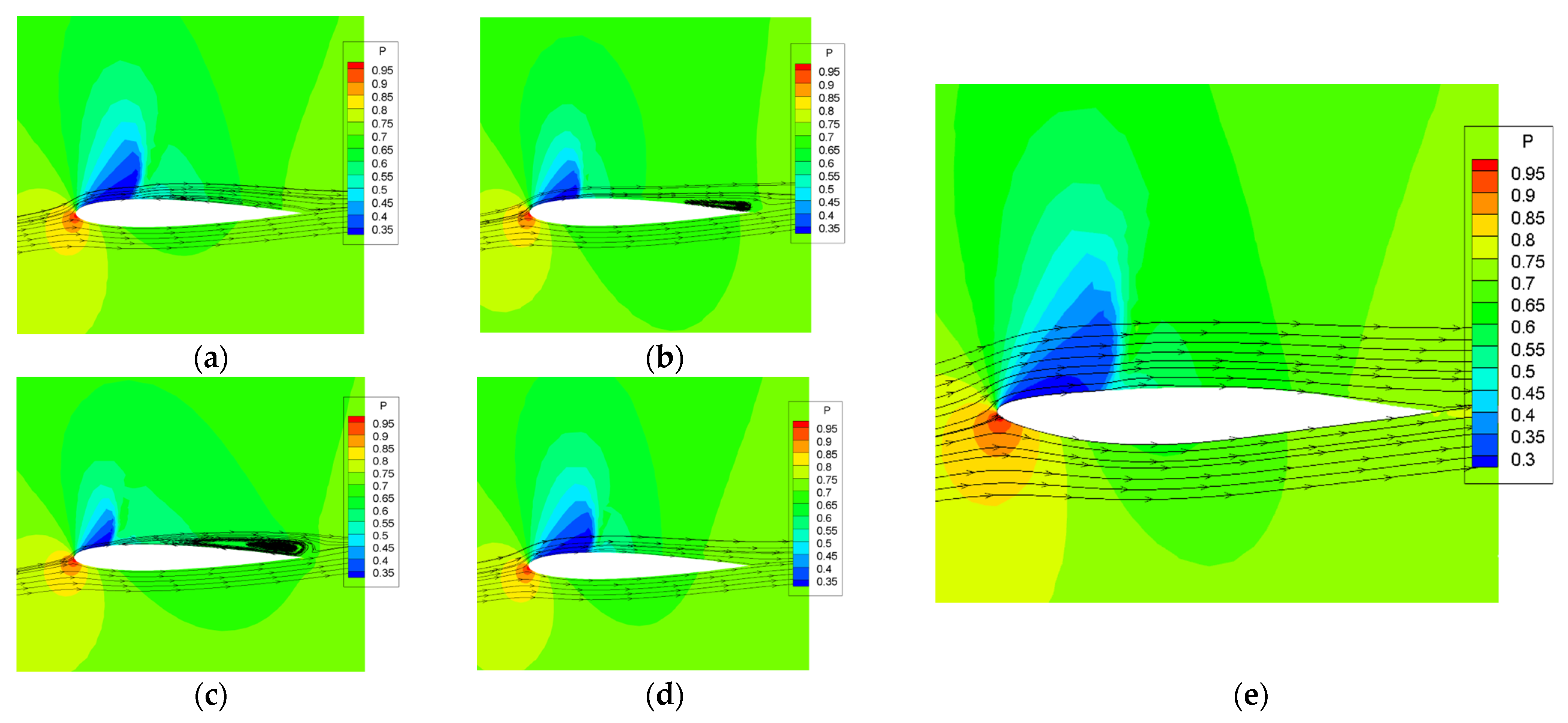
Figure 11 shows the flow field diagrams near the airfoil before and after the optimization of NACA0012.
Figure 11a–d displays the flow field diagrams at four different moments within one buffeting cycle. With the change of time, the shock on the airfoil surface and the separation zone near the trailing edge also change periodically. At moment
, the shock is the closest to the leading edge and the flow separation near the trailing edge is the most intense.
Figure 11e shows the flow field diagram of the optimized airfoil. The optimized airfoil surface flow is stable, and the shock range is expanded compared with the initial airfoil. Because of the narrowing leading edge, the shock position appears to be shifted back, which results in a suction peak at the leading edge of the optimized airfoil and a significant improvement in the aerodynamic performance. Additionally, the flow near the trailing edge is stable, and no flow separation occurs. The buffet is significantly suppressed due to the suppression of the interaction between the shock and the separation zone.
4.2. RAE2822 Airfoil Buffet Optimization
In this section, the transonic buffet optimization is performed for the RAE2822 airfoil. For the optimization of NACA0012, not only the buffet performance but also its steady aerodynamic performance is improved. However, as a typical symmetric airfoil, NACA0012 has poor aerodynamic performance itself in the transonic state, and the optimization can often achieve a large performance improvement. The RAE2822 airfoil, on the other hand, is a supercritical airfoil with superior performance at transonic velocities, and its performance is further improved by the buffet optimization, which proves the advantages of the method.
Set the reinforcement learning reward. Similar to NACA0012, the state with intense buffet is selected as the optimization state, for RAE2822 that is, Ma = 0.75, Re = 1.2 × 10
7, and α = 4.0° [
29]. The specific reward settings are as follows:
In the above equation, the lift coefficient variance is selected as the optimization objective. Similar to the reward setting in the optimization of NACA0012, the lift, drag, and airfoil maximum thickness constraints are set. is the time-averaged value of the lift coefficient after optimization; are the time-averaged value of the lift coefficient, the time-averaged value of the drag coefficient, and the maximum thickness of the airfoil of the initial RAE2822, respectively. The airfoil area is measured after NACA0012 buffet optimization, and a slight reduction is found. Therefore, in the optimization for RAE2822, the airfoil area constraint is added so that the optimized airfoil area is not lower than the initial one (). In addition, the RAE2822 airfoil itself has good lift-drag characteristics. Based on the NACA0012, the weighting factors are adjusted, and , , , and are appropriately reduced to further focus the optimization on the buffet suppression.
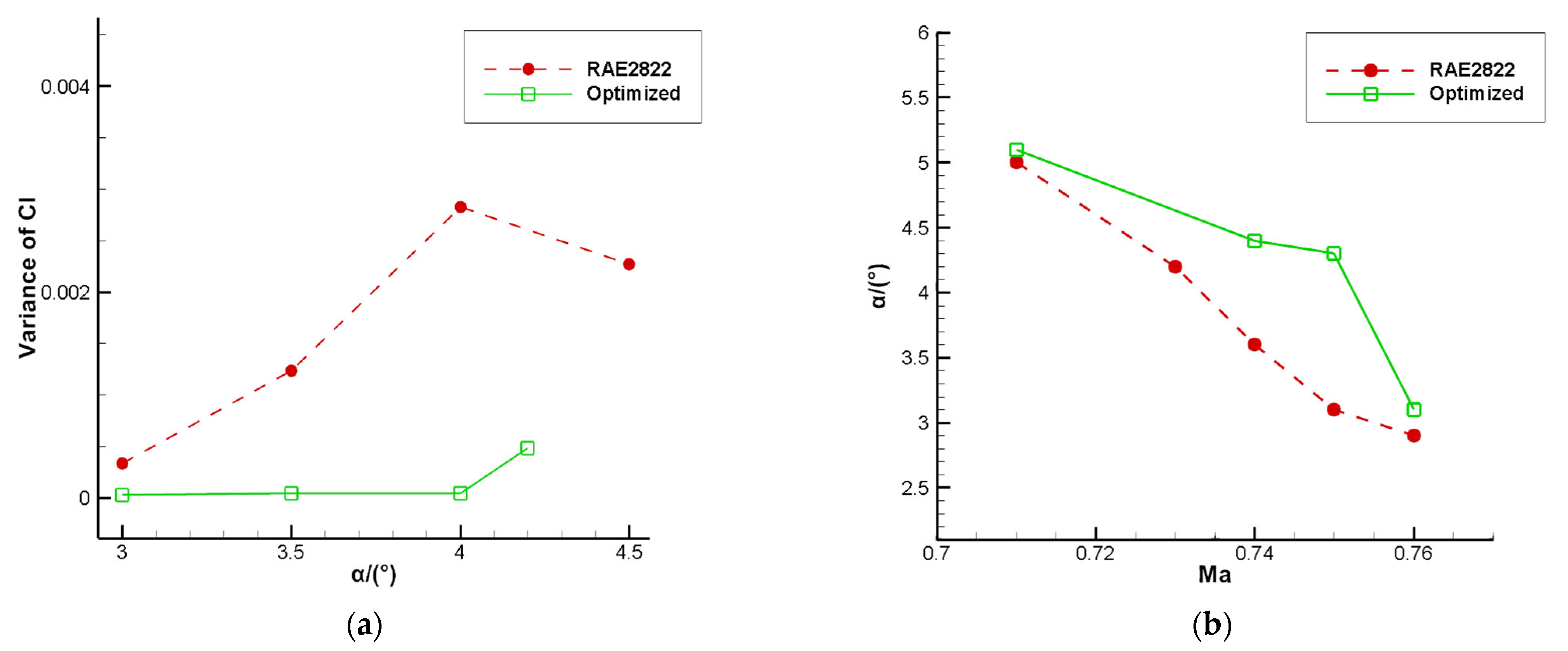
The optimized airfoil buffet is suppressed with the lift coefficient increased and the drag coefficient reduced.
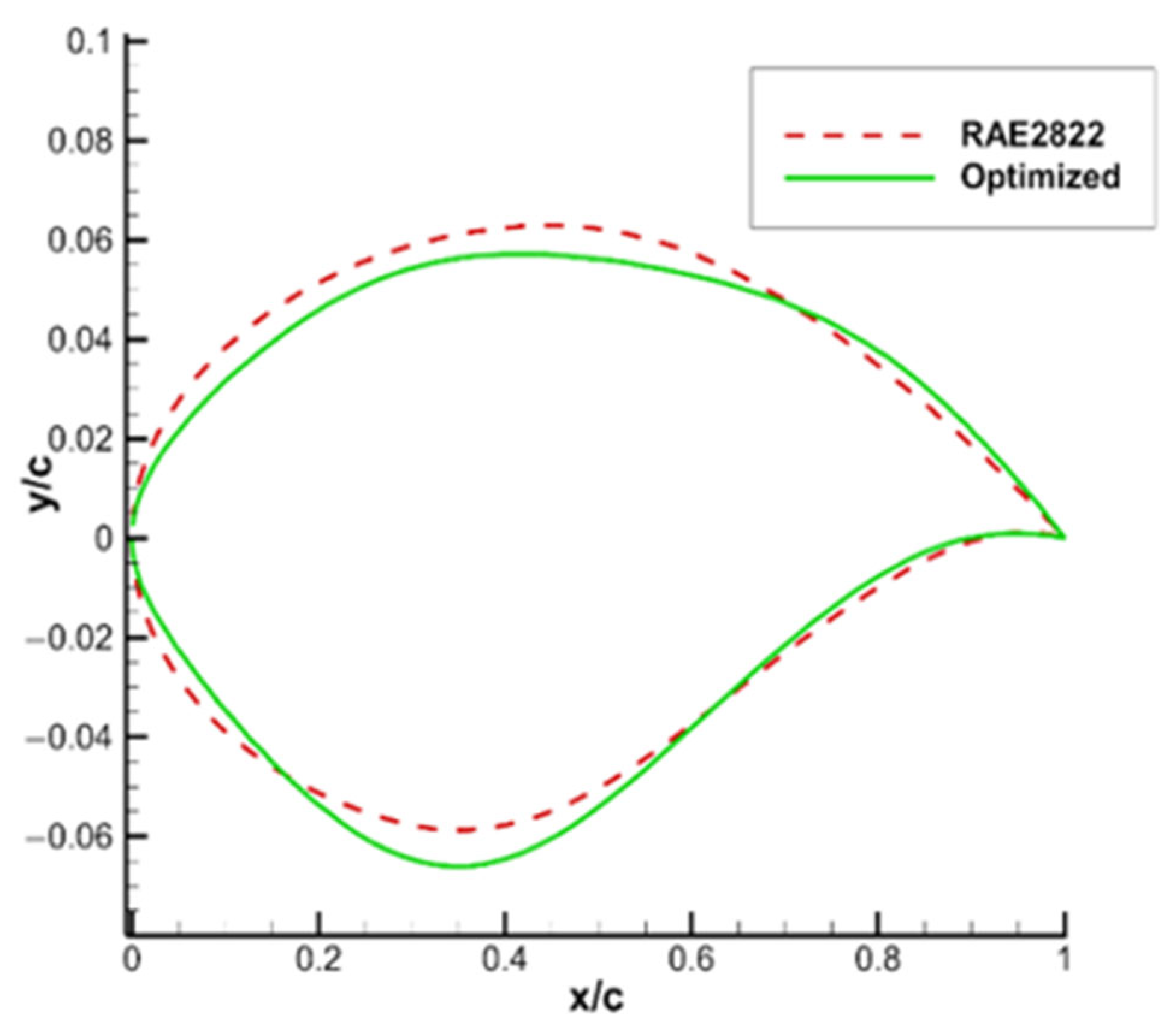
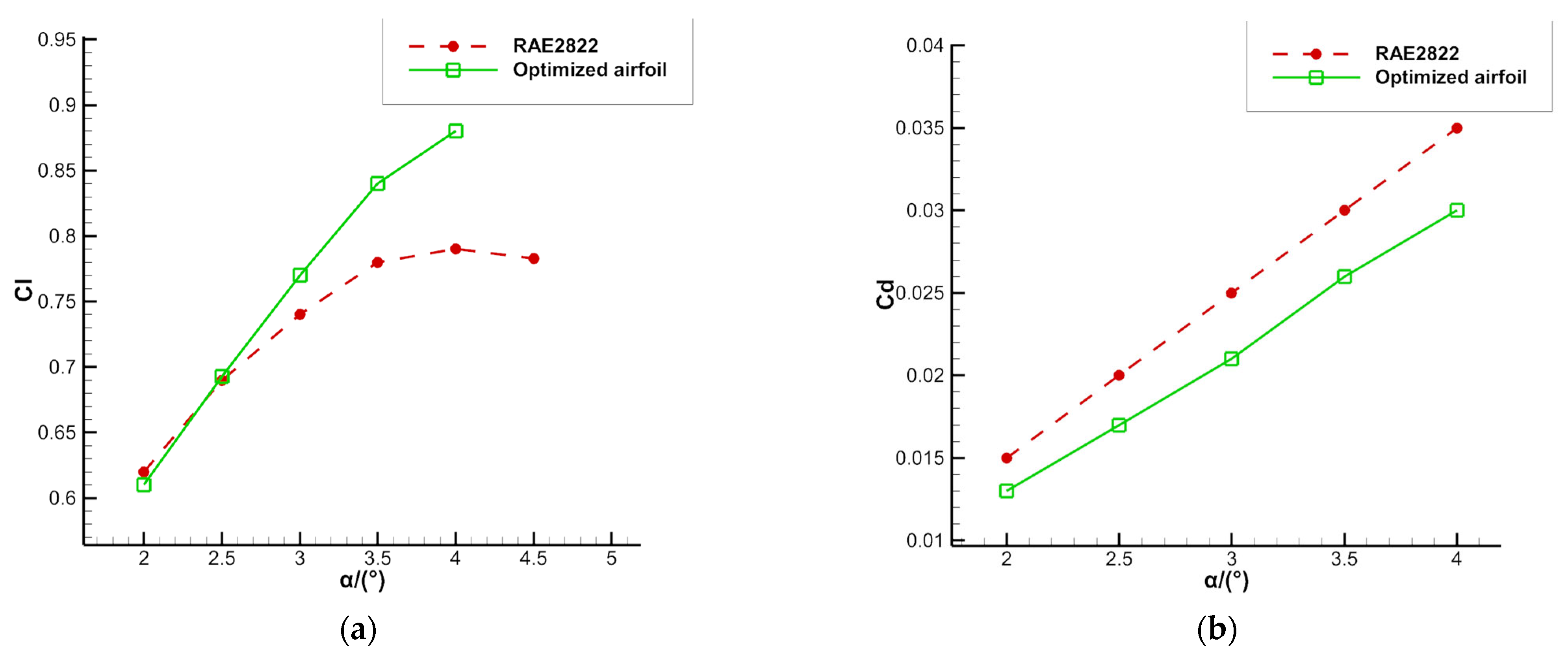
Figure 12 shows the results of the airfoil optimization. Similar to NACA0012, the optimized airfoil shows a narrowing leading edge and a thickening of the trailing edge, with the maximum thickness position appearing at about 0.4 times the chord length. As shown in
Figure 13 and
Figure 14, the optimized airfoil has improved buffet performance and aerodynamic performance. In the optimized state (Ma = 0.75, α = 4.0°, Re = 1.2 × 10
7), the optimized airfoil completely eliminates the buffet and improves the buffet onset boundary, slight buffet occurs at the angle of attack α = 4.2°, and the buffet onset angle of attack boundary is improved by about 1.2°.
Figure 13b shows the buffet optimization result of the RAE2822 airfoil. The optimized airfoil improves the buffet boundary not only in the optimized state, but also in other states.
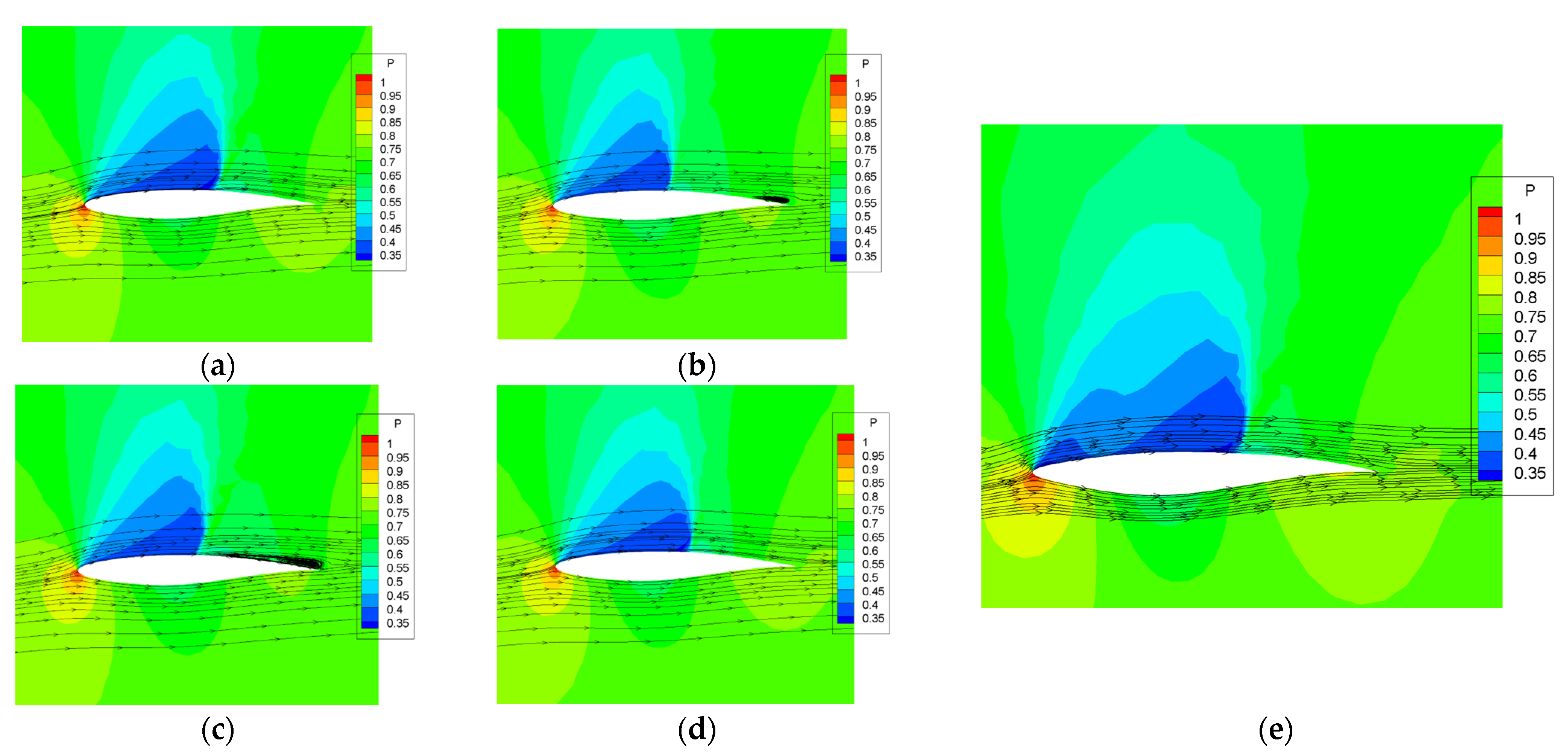
As shown in
Figure 15a–d, in one buffet cycle, the RAE2822 airfoil upper surface shock is closer to the leading edge at
, and the flow separation at the trailing edge is more drastic. After the optimization, the leading edge of the airfoil becomes narrower; the shock is shifted back. Two shock waves appear on the upper surface, and the flow stability increases. In addition, the thickness of the trailing edge is increased, so that the flow separation is limited, and the buffet is eliminated. Before optimization, the strength and area of the shock wave expend when buffet occurs. When buffet is suppressed, there is no flow separation behind the shock foot. This is consistent with the findings of Zhang et al. [
36].
4.3. The Relationship between Buffet and Airfoil Geometric Characteristics
The optimized design results of the buffet for two different airfoils, NACA0012 and REA2822, show that the unsteady aerodynamic shape optimization design method can effectively suppress transonic buffet and significantly improve transonic flow stability. Based on the final optimization results of NACA0012 and REA2822 airfoils, three conclusions can be drawn.
- (1)
The thickness of the leading edge has an influence on the transonic buffet. A narrower leading edge thickness is beneficial to improve the transonic buffet performance, suppress buffet, and improve the flow stability of the airfoil surface.
- (2)
The position of the maximum thickness has an influence on the transonic buffet. In the optimization results of the above two airfoils, the maximum thickness position of the airfoil changes, and it appears near to 0.4 times the chord length.
- (3)
The trailing edge thickness has an influence on transonic buffet. Both the symmetric airfoil NACA0012 and the supercritical airfoil RAE2822 can suppress buffet by increasing the trailing edge thickness of the airfoil in the optimization process of the design for transonic buffet. The flow stability can be increased by appropriately increasing the trailing edge thickness to suppressed the buffet.
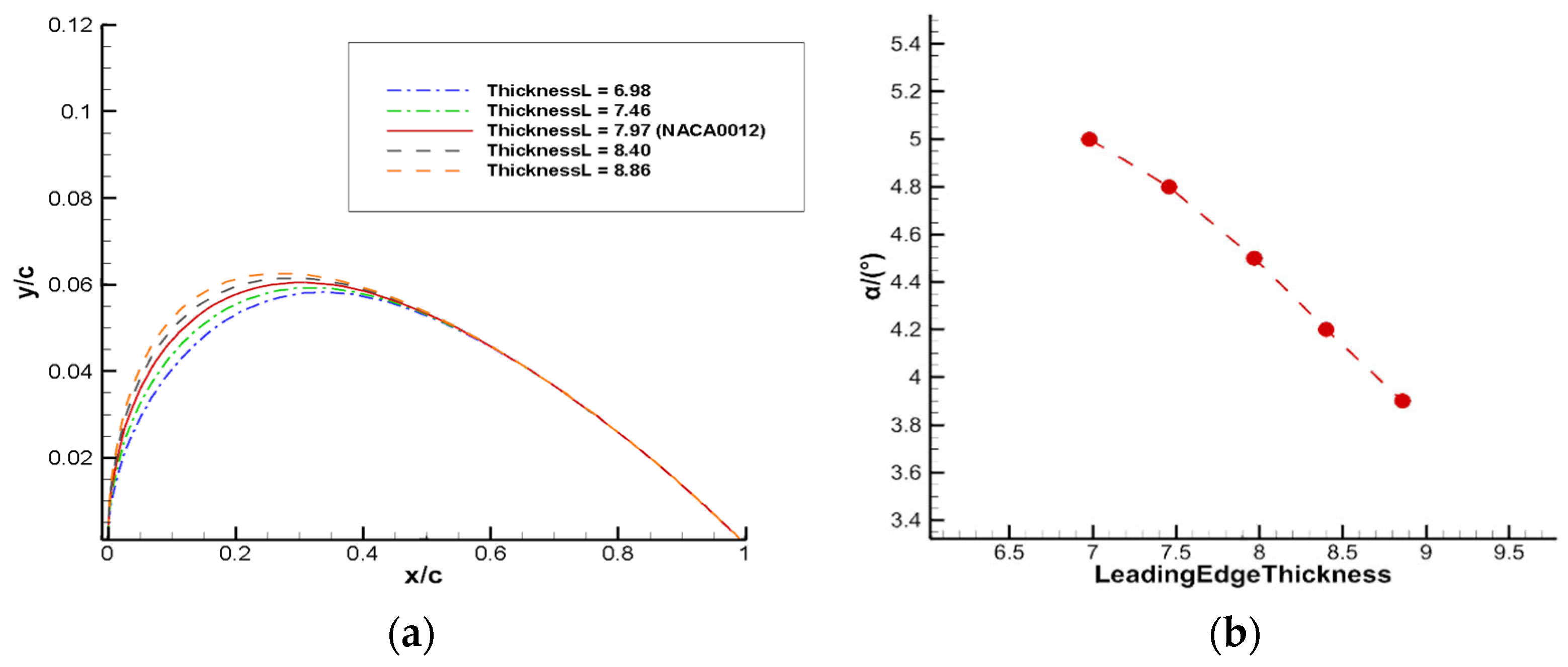
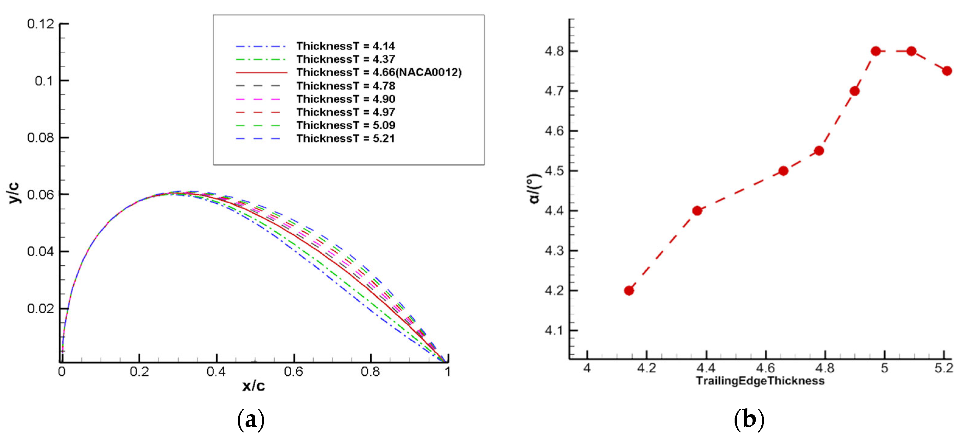
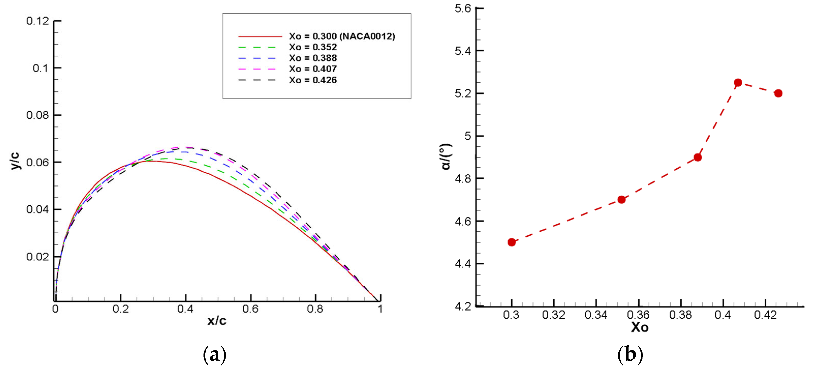
The relationship was investigated between buffet and airfoil geometry characteristics. Although there is consistency in the optimization results of buffet for two airfoils, the conclusions presented above are still specific to these configurations and their generality needs to be further verified. Therefore, this paper further investigated the relationship between buffet and airfoil geometrical characteristics. The effect of airfoil leading edge thickness, trailing edge thickness, and maximum thickness position
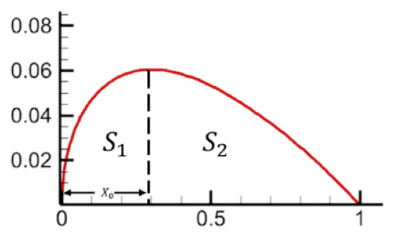
on the buffet performance was investigated in turn by the control variable method. First, the leading edge thickness and trailing edge thickness of the airfoil are quantified as follows:
As shown in the
Figure 16,
is the maximum thickness position, and
and
are the area of the front and back sections of the airfoil respectively.
Airfoil samples are generated by varying the CST parameters of the airfoil. The NACA0012 airfoil is selected as the initial airfoil, and different airfoil samples are generated by changing the leading edge thickness, trailing edge thickness and maximum thickness position of the airfoil, and the buffet performance of these samples is computed. Using the above definition we obtain, the leading edge thickness , trailing edge thickness , and the maximum thickness position for the NACA0012 airfoil.
Figure 17,
Figure 18 and
Figure 19 show the buffet onset boundaries for different airfoil leading edge thicknesses, trailing edge thickness, and maximum thickness positions at Ma = 0.7 and Re = 3 × 10
6. The airfoil samples are kept as symmetric, and only the upper boundary is given in the figure. When the leading edge thickness of the airfoil decreases, the buffet performance is improved, and the angle of attack for the onset of transonic buffet increases. A certain degree of trailing edge thickness increase can also improve the buffet onset boundary, but beyond that range, it does not contribute to the improvement of buffet performance. When the maximum thickness position of the airfoil
, the angle of attack for the onset of buffet increases with the backward shift of the maximum thickness position; and when
, the angle of attack decreases with the backward shift. Therefore, when the maximum thickness position is located near to 0.4 times the chord length, the buffet onset angle of attack of the airfoil reaches its peak and the buffet performance is optimal. This is consistent with the results of the above reinforcement learning-based airfoil buffet optimization.
5. Conclusions and Discussion
The transonic buffet performance of an airfoil is an important aerodynamic index for the lift-drag ratio and is also a hot spot and a difficult area of research in the aviation industry. This paper studied a deep reinforcement learning based approach and constructed a reinforcement learning framework using the DDPG algorithm. The airfoil was parameterized by the CST parameterization method and a CFD program constructed based on the URANS equation for airfoil aerodynamic performance calculation. The buffet optimization design study was carried out for the symmetric airfoil NACA0012 and the supercritical airfoil RAE2822. With the lift coefficient pulsation strength as the key design index, a suitable design state was selected. Through the reinforcement learning based airfoil transonic buffet optimization design study, the buffet optimization of the airfoil was completed without a priori knowledge, and the buffet performance was significantly improved.
In the transonic buffet optimization design study for NACA0012, the optimized airfoil shows a large improvement in buffet performance. Compared with the initial airfoil, there is a 2° increase in the buffet onset angle of attack, and the buffet intensity is significantly lower than that of the initial airfoil. In addition, the steady aerodynamic performance of the airfoil such as lift and drag was also significantly improved. Under the optimized state of Ma = 0.7, α = 5.5° and Re = 3 × 10⁶, the lift coefficient of the airfoil was increased from 0.561 to 0.776, an increase of 38.3%, and the drag coefficient reduction was 33.1%. Meanwhile, in the buffet optimization for RAE2822, the optimized airfoil buffet onset boundary was improved by 1.2°. The steady aerodynamic performance was also improved, with the lift coefficient increasing by 13.9%, from 0.79 in the initial airfoil to 0.88, and the drag coefficient decreasing from 0.035 to 0.030, a reduction of 14.3%.
The results of the airfoil buffet optimization show that there is a connection between the airfoil geometric characteristics and transonic buffet. The airfoil maximum thickness position, leading edge thickness, and trailing edge thickness all affect the fluid flow stability on the airfoil surface. This leads to three general conclusions below related to the airfoil transonic buffet optimization. First, when the airfoil leading edge becomes narrower, the shock moves back and the flow separation near the trailing edge is suppressed. Therefore, the flow stability increases and the buffet is suppressed. Second, when the airfoil trailing edge is thickened within a certain range, the flow separation near the trailing edge is also suppressed, and the buffet performance is improved, however, when the trailing edge thickness 5, the buffet performance decreases. Third, the maximum thickness position also affects the buffet performance, and when it is near 0.4 times the chord length, the buffet onset angle of attack is the largest, and the buffet performance is the best.
Compared with the traditional buffet control method [
37], this study constructively combines buffet optimization with reinforcement learning shape optimization design. Unlike most studies on reinforcement learning based aerodynamic shape optimization design, which focus on the optimization of steady aerodynamic performance such as lift-drag in a steady state, this paper is aimed at the study of transonic buffet in an unsteady state. At the same time, the optimization framework built in this paper, which has the advantages of high transferability and efficiency, can be used for other aerodynamic optimizations of aircraft. In addition, reinforcement learning is computationally superior to the global optimization algorithms. For general aerodynamic shape optimization problems, global optimization algorithms often require hundreds or thousands of CFD calls, and the computational cost increases dramatically when high-dimensional problems are involved. In contrast, reinforcement learning has a strong learning induction capability, and so the number of CFD calls in the optimization process is fewer. Therefore, the efficiency of traditional global optimization algorithms is much lower than that of reinforcement learning, which limits their application in many engineering fields. Although the use of surrogate models can significantly improve the optimization efficiency [
38,
39,
40,
41], it is difficult to build surrogate models on unsteady flow problems, including buffet. The flow field possesses dynamic and complex characteristics. Reinforcement learning has the ability to adjust optimization strategies based on changes in the environment. When applied to aerodynamic shape optimization, it enables adaptive behavior within the flow field. Furthermore, reinforcement learning does not require prior knowledge of the mathematical model of the problem, making it easier to construct an optimization framework.
There is room for improvement. In the buffet optimization process, the buffet criterion mainly relies on CFD calculation, which makes the optimization process more computationally expensive. The optimization process can be further accelerated through the automatic extraction and judgment of transonic buffet features in a data-driven framework. In addition, the flow field information is not fully utilized. The optimization efficiency can be improved by using the buffet flow field characteristics as the optimization variables, extracting the design index from the flow field, and realizing the accurate regulation of the flow field. In recent years, dynamic mode decomposition (DMD) [
42] has been widely used to extract the coherent structure of complex flows and to construct a reduced-order model of flow field evolution [
43]. During the numerical simulation process, DMD can accelerate the convergence of the flow field [
44,
45] and reduce the CFD computational costs. Moreover, neural networks have the ability to learn complex nonlinear relationships, process and analyze large amounts of data, and extract buffet features from the flow field. Therefore, it can also improve the optimization efficiency. Our next step is to develop efficient convergence methods to accelerate buffet numerical simulations, which are of great engineering importance, to improve the optimization efficiency of reinforcement learning-based aerodynamic shape optimization design.


