Time-Inclined Method for High-Fidelity Rotor/Stator Simulations

Abstract

The application of the time-inclined method in a fourth-order unstructured flux-reconstruction code for turbomachinery is demonstrated. Inviscid and viscous unsteady results due to the interaction of an incoming gust of total pressure with a linear cascade of flat plates and a linear cascade of T106A low-pressure turbine airfoils are reported. The agreement between the time-inclined method and the equivalent full-annulus multipassage solution is very high for both cases. Viscous solutions at Reynolds numbers of ${10}^4$ and ${10}^5$ were conducted. A high degree of matching was obtained between the time-inclined and the whole annulus approaches. The limitations of the method are explored and discussed. While the evolution of the unsteady boundary layers created by the interaction with the incoming wakes was very well captured, the mixing associated with the trailing edge vortex shedding was less accurate. The critical parameter controlling the method’s accuracy is the local Strouhal number. It was demonstrated that the benefit of retaining the exact blade count in the simulations overcomes the slight differences in the mixing due to the limitation of the time-inclined method to model viscous effects accurately in all situations.

1. Introduction

Scale-resolving simulations have evolved up to a point in which they can compete with low technology readiness level (TRL) experiments [1,2]. A substantial fraction of the fine scales are appropriately resolved, often without any modelling, and the computational cost is affordable at the industrial level for quasi-three-dimensional simulations at moderate Reynolds numbers ($Re\sim {10}^5$) provided that they are restricted to a single passage. However, the long spatial scales associated with the blade count disparity between stators and rotors play a significant role in aeroelastic and aeroacoustics problems, making it convenient to retain the exact blade count of the airfoil and its perturbations in eddy-resolving simulations. Moreover, keeping the exact blade count of the incoming wakes is relevant for the mixing process and avoids modifying the flow parameter of the simulations as well.

Virtual experiments reproducing the losses of linear cascades with moving bars are beginning to become commonplace [1,2,3,4,5]. Nonetheless, the simulations accuracy is frequently compromised to accommodate the blade count to a single passage. For instance, in the experiment reported by Bolinches et al. [2], the actual ratio between the pitch of the rotating bars and the airfoils was $P_r/P_s=1.07$, but it was approximated to $P_r/P_s=1$ in the simulations. Moreover, the bar speed was adjusted to match the bar passing frequency changing the experimental flow parameter. This is not an option for realistic blade counts, and this approach contradicts performing computationally intensive high-fidelity simulations since, at the same time, the physical parameters of the simulations are approximated grossly.

The problem is further aggravated in scale-resolving simulations to predict fan broadband interaction noise. In this case, the blade count of the single fan stage is frequently approximated to reduce the size of the computational domain [6,7]. Although the impact can be small for broadband noise predictions, it does affect the aerodynamics and the generation of pure tones hindering the holistic nature of the simulation. Generally speaking, although the impact of adjusting the number of incoming wakes in the aerodynamic loss predictions can be small, the same is not valid in the acoustic field.

One of the main bottlenecks for a generalised application of high-fidelity simulations in the industry lies in the difficulties encountered when the stator/rotor pitch ratio is not a small integer ratio. In this case, spatial periodicity is only recovered by including many blade passages in the computational domain, significantly reducing the affordability of the simulations.

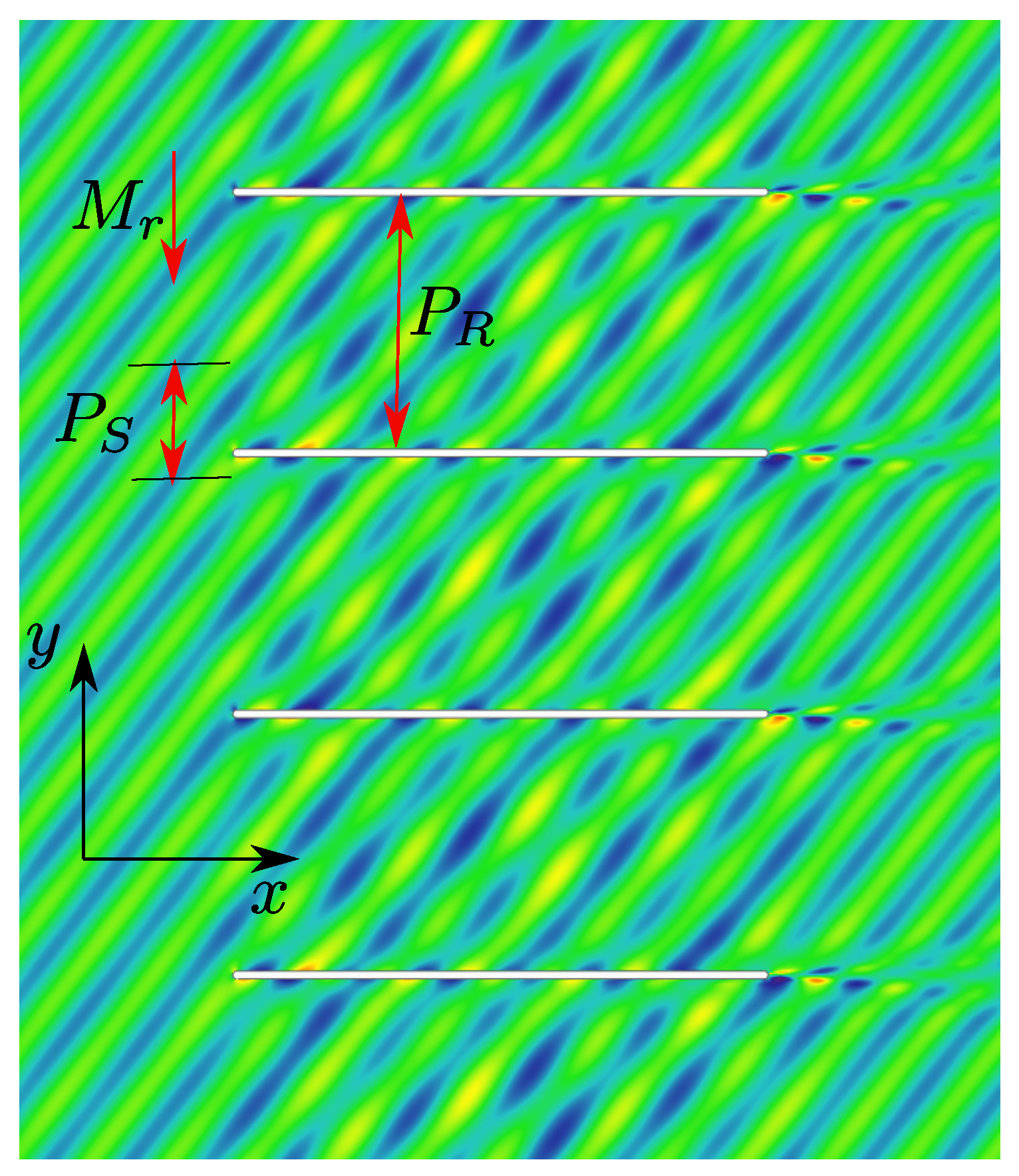
Several methods have been proposed to deal with dissimilar blade counts using a single-passage approach for time-periodic flows. Erdos et al. [8] addressed, for the first time, the problem of the computational efficiency of a stator/rotor interaction with dissimilar pitches between the stator and the rotor (see Figure 1) using a method whereby the solution was reconstructed in the periodic boundaries and the sliding plane, assuming that the solution was periodic in time. This approach was optimised, approximating the stored solution with a truncated Fourier series in time to reduce the amount of storage [9,10] and to account for multiple fundamental frequencies [11].

The strongest hypothesis of the methods mentioned above posits that the harmonic content of the flow is formed by a few fundamental frequencies associated with the blade passing frequencies of the neighbouring rows and their higher-order harmonics [11]. This hypothesis is needed to reconstruct the signal using earlier time instants on the opposite side of the periodic line. Temporal signals from scale-resolving rotor/stator simulations superimpose random-like unsteady contributions to a baseline periodic content of the signal similar to unsteady Reynolds-averaged Navier–Stokes (URANS) simulations, conceptually preventing a direct application of phase-lagged boundary conditions. However, recent attempts have been pursued unsuccessfully [12,13].

The use of phase-shifted boundary conditions experiences two additional problems. The first is a degradation of the convergence time with respect to the full-annulus (FA) simulation, even for URANS analyses. Part of this problem stems from the difficulty in implementing fully consistent phase-lagged boundary conditions in the periodic boundaries. To remedy this problem, Biesinger et al. [14] proposed the dual-passage method whereby the phase-lagged boundary conditions are implemented in two passages instead of a single one to mitigate the convergence problem. Giovannini et al. [15] reported a factor of five in computational time using this technique in a rotor/stator simulation despite using twice as many points as that of the original method. Moreover, in a scale-resolving simulation, the time spectrum is richer than that in URANS simulations, and the number of snapshots that need to be stored in the boundaries is very high.

In the early nineties, Giles [16,17] introduced the use of time-inclined (TI) computational planes to deal with the difficulties encountered with dissimilar stator/rotor pitch ratios. The TI method performs a time transformation of the equations leading to a new set of governing equations. In contrast to the time-harmonic and phase-shifted methods, the TI method does not require the hypothesis of flow periodicity which makes it potentially suitable for the scale-resolving simulation of turbulent flow. One of the main limitations attributed to the TI method is that it can only deal with a single stage (single-pitch ratio) but does not suffer from convergence problems due to the boundary conditions; neither requires additional storage nor makes explicit use of the time periodicity of the flow. The method is limited to specific combinations of pitch ratios and rotor velocities, but typical turbomachinery applications lie within the applicability range. Moreover, it is generally possible to circumvent such limitations by simulating more than a single passage in the reduced domain, yet avoiding the cost of computing a much larger domain with directly periodic boundary conditions. Despite the fact that the time-inclined method was introduced more than 30 years ago, it is not widely implemented in turbomachinery solvers with the sole exception of the ANSYS suite of solvers [18], and therefore its analysis is very limited.

To the authors’ knowledge, this is the first time that the time-inclined method has been implemented in a high-order flux-reconstruction (FR) method, and the accuracy of the TI method is discussed in detail. The discussion concerning the accuracy of the TI method to represent viscous unsteady non-periodic flows is also new and applies to classical second-order RANS solvers as well. The combination of the time-inclined and flux-reconstruction methods is an original solution to tackle the LES or DNS of a single-stage turbomachine with dissimilar blade counts in the rotor and the stator using a single-passage approach. The efficient and accurate simulation of this problem will enable eddy-resolving simulations of at least single-stage configurations, which is a problem that has not been overcome thus far.

This paper first introduces the time-inclined method and the high-order numerical scheme of the baseline solver. It further identifies the conditions under which the accuracy of the TI method is degraded. Following this, two-dimensional results in linear cascades of flat plates and low-pressure turbine (LPT) airfoils are presented. Finally, the paper ends with a discussion on the accuracy of the results and the conclusions.

2. Materials and Methods

2.1. Numerical Method

Because of computational efficiency, low dissipation schemes are used frequently in scale-resolving simulations of turbulent flows instead of standard second-order methods typically used in RANS analysis. Higher-order compact numerical methods, such as the flux reconstruction method (FR), offer low numerical dissipation and are well-suited for simulating vortical structures and turbulent flows [19].

The time-inclined method has been integrated into a compressible high-order solver [20,21] based on the FR method of Huynh [22] and extended to triangular elements following the work of Wang and Gao [23]. The technique has been successfully used to perform quasi-direct numerical simulations of low-pressure turbine transitional flows in the presence of incoming wakes [1,2]. A summary of the numerical method is given next for the sake of completeness.

Spatial Discretization

The FR method [22] for the solution of one-dimensional conservation laws

$$\frac{\partial \mathbf{U}}{\partial t}+\frac{\partial \mathbf{f}}{\partial x}=0$$

(1)

is revisited first. Consider a 1D integration domain $\Omega =\left[0,L\right]$ discretized in N elements with the ith element defined by $V_i=[x_i,x_{i+1}]$. For each element i, we define $p+1$ solution points (SPs) at which the state variable ($\mathbf{U}$) is evaluated. Given these SPs, the solution is approximated using Lagrange polynomials as

$$\mathbf{U}(x,t)\simeq {\mathbf{U}}_i^h(x,t)=\sum _{j=1}^{p+1}{\mathbf{U}}_{ij}^h\left(t\right)L_j\left(x\right)$$

(2)

where ${\mathbf{U}}_{ij}^h$ is the solution at SP j of element i, and $L_j\left(x\right)$ is the Lagrange polynomial with value 1 at $x=x_j$. For each element, we define a local coordinate, $\xi =\left[-1,1\right]$, such that $x_j=x_i+\frac{▵x_i}{2}\left({\xi }_j+1\right)$ with $\Delta x_i=x_{i+1}-x_i$. The flux is defined analogously:

$$\mathbf{f}\left({\mathbf{U}}^h\right)\simeq {\mathbf{f}}_i^D(\xi ,t)=\sum _{j=1}^{p+1}\mathbf{f}\left({\mathbf{U}}_{ij}^h\right)L_j\left(\xi \right)$$

(3)

Since the solution is in general discontinuous across element interfaces, the flux is reconstructed in such a way that the reconstructed flux ${\mathbf{f}}^C$: (i) is of degree $p+1$, where p is the order of ${\mathbf{f}}^D$, (ii) is close to ${\mathbf{f}}^D$, and (iii) takes the value of the interface fluxes at the boundaries of the element which is computed with a Riemann solver. The final corrected flux is of the form ${\mathbf{f}}_i^C\left(\xi \right)={\mathbf{f}}_i^D\left(\xi \right)+{\gamma }_i\left(\xi \right)$ where ${\gamma }_i\left(\xi \right)$ is the correction flux function defined as follows:

$${\gamma }_i\left(\xi \right)=[{\mathbf{f}}_L^I-{\mathbf{f}}^D(\xi =-1)]g_L\left(\xi \right)+[{\mathbf{f}}_R^I-{\mathbf{f}}^D(\xi =1)]g_R\left(\xi \right)$$

(4)

where ${\mathbf{f}}_L^I$ and ${\mathbf{f}}_R^I$ are the left and right interface fluxes, and $g_L\left(\xi \right)$ and $g_R\left(\xi \right)$ are the left and right correction functions, respectively. The correction functions are chosen as the left and right Radau polynomials in this work to recover the nodal-based discontinuous Galerkin formulation. The discrete form of Equation (1) is as follows:

$${\displaystyle \frac{\partial \mathbf{U}}{\partial t}}+{\displaystyle \frac{\mathrm{d}\xi }{\mathrm{d}x}}\left\{\sum _{j=1}^{p+1}\mathbf{f}\left({\mathbf{U}}_{ij}^h\right){\displaystyle \frac{\mathrm{d}{L}_j}{\mathrm{d}\xi }}\left(\xi \right)+[{\mathbf{f}}_L^I-{\mathbf{f}}^D(\xi =-1)]{\displaystyle \frac{\mathrm{d}{g}_L}{\mathrm{d}\xi }}\left(\xi \right)+\left.[{\mathbf{f}}_R^I-{\mathbf{f}}^D(\xi =1)]{\displaystyle \frac{\mathrm{d}{g}_R}{\mathrm{d}\xi }}\left(\xi \right)\right\}=0\right.$$

(5)

which is advanced in time using a fourth-order Runge–Kutta scheme.

The extension to multiple dimensions of the method is readily performed for quadrilateral elements as tensor product operations in multiple dimensions. The extension of the method to triangular elements is performed using the correction procedure by reconstruction (CPR) approach of Wang and Gao [23].

2.2. Time-Inclined Formulation

The formulation of the time-inclined method has been described previously [16] but is summarised below for the sake of completeness.

2.2.1. Euler Equations

The two-dimensional Euler equations in the physical coordinate system can be written in a conservative form as follows:

$$h\frac{\partial \mathbf{U}}{\partial t}+\frac{\partial \left(h\mathbf{f}\right)}{\partial x}+\frac{\partial \left(h\mathbf{g}\right)}{\partial y}=\mathbf{S},$$

(6)

where

$$\mathbf{U}=\left(\begin{array}{c}\rho \\ \rho u\\ \rho v\\ \rho E\end{array}\right),\mathbf{f}=\left(\begin{array}{c}\rho u\\ \rho u^2+p\\ \rho uv\\ \rho uH\end{array}\right),\mathbf{g}=\left(\begin{array}{c}\rho v\\ \rho uv\\ \rho v^2+p\\ \rho vH\end{array}\right)$$

(7)

and h is the streamtube thickness of the two-dimensional section that gives rise to the source term $S={\left(0p{h}_{x}p{h}_{y}0\right)}^T$ in the right-hand side of Equation (6). Giles considered a transformation from the physical coordinates $(x,y,t)$ to the computational coordinates $(x^{\prime },y^{\prime },t^{\prime })$ such that periodicity is achieved in the rotor and stator computational domains (see Figure 1), i.e., $U(x,y,t)=U(x,y+P_r,t+\Delta T)$.

The equations defining the transformation are

$$x^{\prime }=x,y^{\prime }=y,\tau =t-\lambda y$$

(8)

where

$$\lambda =\frac{\Delta T}{P_r}=\frac{P_s-P_r}{V{P}_r}.$$

(9)

This transformation can be regarded as grid mapping analogous to that performed to map the governing equations from the physical domain to the transformed domain in structured solvers. The main difference is that time is deemed one more dimension and transformed in the mapping process. The resultant system of equations in the computational coordinate system is as follows:

$$\frac{\partial \mathbf{Q}}{\partial \tau }+\frac{\partial \mathbf{f}}{\partial x^{\prime }}+\frac{\partial \mathbf{g}}{\partial y^{\prime }}=\mathbf{S},$$

(10)

where the new conservation variables are $\mathbf{Q}=\mathbf{U}-\lambda \mathbf{g}$. This redefinition of the conservation variables causes a minimum disruption in the baseline numerical method because $\mathbf{U}$ can be calculated from $\mathbf{Q}$ in closed form for a perfect gas. This is particularly useful in GPU-based codes where increasing the number of operations per point is computationally forgiven. For explicit codes, the main idea is to advance the new conservative variables to the next time step ${\mathbf{Q}}^{n+1}$, then compute ${\mathbf{U}}^{n+1}=ϝ\left({\mathbf{Q}}^{n+1}\right)$, and finally, re-evaluate the original physical fluxes in the time instant $(n+1)\Delta t$, i.e., ${\mathbf{f}}^{n+1}=\mathbf{f}\left({\mathbf{U}}^{n+1}\right)$ and ${\mathbf{g}}^{n+1}=\mathbf{g}\left(U^{n+1}\right).$

With a departure from the values of $\mathbf{Q}={(q_1,q_2,q_3,q_4)}^T$, the relationship between $\mathbf{Q}$ and $\mathbf{U}$ can be written as follows:

$$\begin{array}{cc}{q}_1=\hfill & \rho (1-\lambda v)\hfill \\ q_2=\hfill & q_{1}u\hfill \\ q_3=\hfill & q_{1}v-\lambda p\hfill \\ q_4=\hfill & \frac{1}{2}{q}_1(u^2+v^2)+\frac{1}{\gamma -1}p-\lambda \frac{\gamma }{\gamma -1}{\displaystyle pv}\hfill \end{array}$$

(11)

By injecting $u=q_2/q_1$ and $v=(q_3+\lambda p)/q_1$ from the second and third equations into the fourth equation, the following equation for the static pressure is obtained:

$$a{p}^2+2bp+c=0$$

(12)

where

$$\begin{array}{c}a=(\gamma +1){\lambda }^2\\ b=-(q_1-\lambda q_3)\\ c=(\gamma -1)(2q_1{q}_4-(q_2^2+q_3^2))\end{array}$$

(13)

The quadratic equation has two solutions:

$$p=\frac{1}{a}\left(-b\pm \sqrt{b^2-ac}\right)$$

(14)

The negative root yields the correct value for $\lambda \to 0$. Once p is obtained, the remaining physical variables can be easily obtained.

2.2.2. Navier–Stokes Equations

The 2D Navier–Stokes equations can be written in conservative form and in the physical coordinate system as follows:

$$h\frac{\partial \mathbf{U}}{\partial t}+\frac{\partial \left(h\mathbf{f}\right)}{\partial x}+\frac{\partial \left(h\mathbf{g}\right)}{\partial y}=\frac{\partial \left(h\mathbf{F}\right)}{\partial x}+\frac{\partial \left(h\mathbf{G}\right)}{\partial y}+\mathbf{S}$$

(15)

where

$$\mathbf{F}=\left(\begin{array}{c}0\\ {\tau }_{xx}\\ {\tau }_{yx}\\ {\tau }_{xx}u+{\tau }_{xy}v-q_x\end{array}\right),\mathbf{G}=\left(\begin{array}{c}0\\ {\tau }_{xy}\\ {\tau }_{yy}\\ {\tau }_{yx}u+{\tau }_{yy}v-q_y\end{array}\right)$$

(16)

where the stress tensor is given by

$$\tau =\mu (\nabla \mathbf{v}+\nabla {\mathbf{v}}^T)-\frac{2}{3}\mu \mathbf{I}\nabla ·\mathbf{v}$$

(17)

where $\mu$ is the dynamic viscosity, and $\mathbf{I}$ is the identity matrix. The heat flux vector is given by $\mathbf{q}=\kappa \nabla T$, where $\kappa$ is the conductivity.

The application of the time-inclined transformation to Equation (15) leads to

$$h\frac{\partial \mathbf{Q}}{\partial t}+\frac{\partial \left(h\mathbf{f}\right)}{\partial x^{\prime }}+\frac{\partial \left(h\mathbf{g}\right)}{\partial y^{\prime }}=\frac{\partial \left(h\mathbf{F}\right)}{\partial x^{\prime }}+\frac{\partial \left(h\mathbf{G}\right)}{\partial y^{\prime }}+\mathbf{S}$$

(18)

with $\mathbf{Q}=\mathbf{U}-\lambda (\mathbf{g}-\mathbf{G})$. The problem now is that $\mathbf{Q}$ contains temporal and spatial derivatives of $\mathbf{U}$, and a direct relationship $\mathbf{U}=ϝ\left(\mathbf{Q}\right)$ does not exist. To circumvent this problem, $\mathbf{Q}$ is replaced by $\mathbf{U}-\lambda \mathbf{g}$ which can be shown to be a valid approximation for flows with low locally reduced frequencies [24].

2.2.3. Time-Inclined Method Limitations

The TI method is not exact for unsteady viscous flows. The question that remains to be answered is under which circumstances the TI method is an acceptable approximation for the Navier–Stokes equations. To clarify this point, let us consider the momentum equation in the TI plane:

$$\begin{array}{c}\hfill (1-\lambda v){\displaystyle \frac{\partial \mathbf{v}}{\partial t}}+\mathbf{v}\nabla \mathbf{v}=-{\displaystyle \frac{1}{\rho }}\nabla p-\lambda p_t\mathbf{j}+\nu (\underset{\left(4\right)}{{\nabla }^2\mathbf{v}}-\underset{\left(5\right)}{2\lambda {\displaystyle \frac{{\partial }^2\mathbf{v}}{\partial t\partial y^{\prime }}}}+\underset{\left(6\right)}{{\lambda }^2{\displaystyle \frac{{\partial }^2\mathbf{v}}{\partial t^2})}}\end{array}$$

(19)

The first line corresponds to the inviscid terms, which are transformed exactly. However, the unsteady viscous terms (5) and (6) are not resolved within the framework of the TI method, and they will be regarded as error terms since they become null when $\lambda =0$. The order of magnitude of the term (5) with respect to (4) is

$$\frac{\left(5\right)}{\left(4\right)}\sim \frac{\lambda v_c{f}_c/L_c}{v_c/L_c^2}\sim \lambda f_c{L}_c=St$$

(20)

where $f_c$ is the characteristic frequency, and $St=fL/v$ is the Strouhal number of the problem being confronted. The time inclination parameter $\lambda$ has the units of the inverse of a velocity, and for stability reasons, $\tilde{\lambda }=\lambda v_{\mathrm{exit}}$ is at most of the order unity, i.e., $\tilde{\lambda }\sim \mathcal{O}\left(1\right)$, being $v_{\mathrm{exit}}$ the exit velocity of the cascade. The characteristic speed of the problem is $v_c$, and so, analogously, the order of magnitude of the term (6) with respect to the (4) is as follows:

$$\frac{\left(6\right)}{\left(4\right)}\sim \frac{{\lambda }^2{v}_c{f}_c^2}{v_c/L_c^2}\sim {\left(\lambda f_c{L}_c\right)}^2=S{t}^2$$

(21)

Therefore, this term is higher or lower than is term (5) depending on whether $St$ is greater or less than one.

Inlet Region and Airfoil Passage

It will be assumed that the reduced frequency of the forcing $S{t}_f=f_{f}c/v_{\mathrm{exit}}\sim \mathcal{O}\left(1\right)$ where $f_f$ is the frequency of the incoming perturbation, and c is the airfoil chord which is typically similar to the airfoil pitch. This effectively means that the decay of the incoming wake due to viscous effects is altered in the TI plane. However, this impact is small for high Reynolds number flows since the wake decay between the trailing edge of the preceding airfoil and the leading edge, as well as along the airfoil passage, is small since $S{t}_{f}R{e}_f\gg 1$. The Rapid Distortion Theory (RDT) [25] of turbulence requires the same condition, which essentially states that vortices pass through the cascade without attenuation or interaction since the diffusion time is much longer than is the residence time in the airfoil. The RDT assumption has been used successfully in broadband rotor/stator interaction noise simulations [26,27].

Laminar Boundary Layers

The characteristic length of a laminar boundary layer (BL) is its thickness, $\delta$, which is much smaller than the characteristic length of the perturbations that is taken as the chord. The characteristic velocity in the boundary layer is $v_{\mathrm{exit}}$ since this is the origin of the shear in the BL. The characteristic time of the oscillations in the BL is the same as that of the forcing, and hence

$$S{t}_{BL}=\frac{f_f\delta }{v_{\mathrm{exit}}}=S{t}_f\frac{\delta }{c}\sim S{t}_f\frac{1}{R{e}_c^{1/2}}$$

(22)

which is small if the Reynolds number is high enough. The conclusion is that the evolution of an unsteady laminar boundary layer is properly resolved using the TI transformation.

Vortex Shedding

In this case the characteristic length is the trailing edge thickness, $t_{TE.}$, which is typically similar to the boundary layer thickness, $t_{TE}\sim \delta$. The main difference here is that the frequencies associated with the flow oscillation in the TE are much higher than those of the forcing since

$$S{t}_{TE}=\frac{f_{TE}{t}_{TE}}{v_{\mathrm{exit}}}\sim \mathcal{O}\left(1\right)$$

(23)

The neglected viscous terms are as important as the retained terms, so the approximation is inconsistent. It will be shown that discrepancies between the exact and the TI solution in the mixing process behind a 2D plate can be noticed due to this problem.

3. Results

Several test cases were conducted to assess the accuracy of the implementation and the approach. A pair of two-dimensional linear cascades, the first being flat plates and the second being T106A [28] airfoils, were chosen as the testing vehicles. It is important to remark that comparing a single-passage method with the equivalent full-annulus solution in a high-order code can be a daunting task due to the sensitivity of the solution to the details of the numerics.

3.1. Flat-Plate Linear Cascade

A linear cascade of flat plates with zero stagger angle and a pitch-to-chord ratio of $P_s/c=0.5$ was used to test the implementation. The exit Mach number of the cascade is $M_2=0.39$, and the incidence is null. The cascade has a finite thickness t to ease the mesh generation process ($t/c=1.5\%$). The plate is considered a rotor passing downstream of a row of stators with pitch $P_s$. The ratio between the number of stators, $N_s$, and rotors, $N_r$, is $N_s/N_r=15/6$, and therefore, the simulation does not fit into a single passage. The computational domain of the full annulus simulation (with direct periodicity) consists of six plates in this particular case. The domain is discretized using a hybrid grid of fourth-order triangles and quads. The equivalent second-order mesh consists of 100 points on the plate and 20 on the leading and trailing edges. The boundary layer regions are discretized with four quad layers (16 points in the fourth-order mesh), and the whole mesh totals 13,500 cells per passage. The full-annulus computational domain is constructed replicating the mesh of a single passage. This eliminates some of the spatial discretization differences between the time-inclined and full-annulus simulations since the mesh per passage is identical. A sinusoidal perturbation of 2.5% of the inlet total pressure is imposed at the inlet, giving rise to a mix of pressure, vortical, and entropy waves. The dimensionless speed of the rotor is $M_r=0.52$. The combination of the rotor speed and the number of perturbations gives rise to a high blade-passing reduced frequency $k=\omega c/v_{2,is}=40.4$. See Figure 2 for a general setup description. The unusually high value of the reduced frequency was chosen to magnify the errors created by the viscous terms in TI transformation.

3.1.1. Inviscid Case

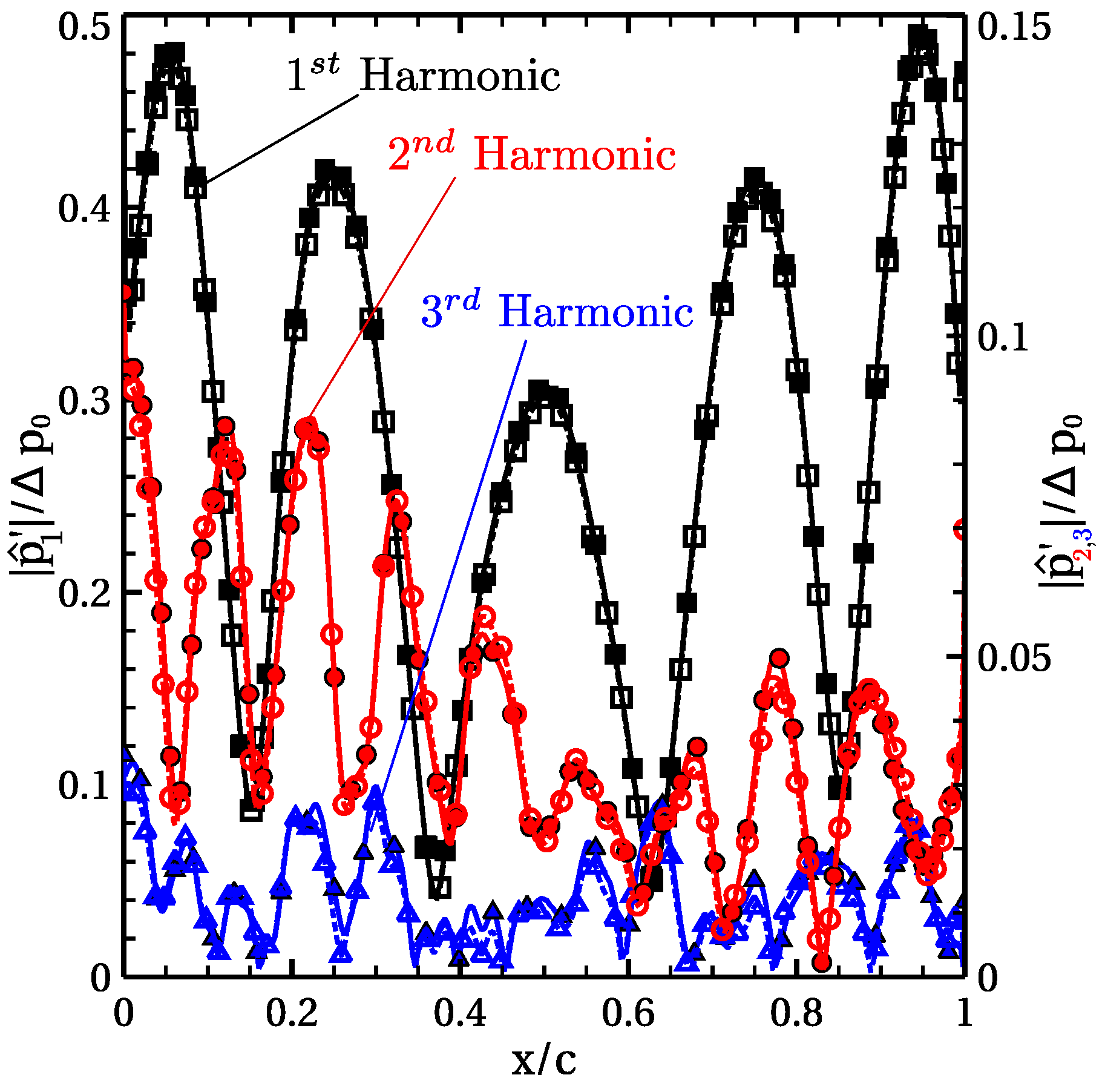
Figure 3 compares the normalized modulus (normalized amplitude of the complex unsteady perturbations) of the first three harmonics of the static pressure $\left|{\widehat{p}}_1^{\prime }\right|$, $\left|{\widehat{p}}_2^{\prime }\right|$ and $\left|{\widehat{p}}_3^{\prime }\right|$, on the lower side of the plate obtained by a full-annulus analysis and the time-inclined method. The static pressure can be expressed as the sum of a mean flow and an unsteady perturbation,

$$p(x,y,t)=\overline{p}(x,y)+p^{\prime }(x,y,t)=\overline{p}(x,y)+\mathrm{Re}\left({\widehat{p}}_n^{\prime }{e}^{I2\pi {\omega }_{n}t}\right),$$

(24)

where ${\widehat{p}}_n^{\prime }$ is the n-th complex Fourier coefficient of the pressure.

Solid lines and filled symbols correspond to the full-annulus analysis, whereas the time-inclined solution is represented with dotted lines with empty symbols. The degree of agreement between both approaches is very high, and it is an indication that the solution is converged. It must be recalled at this point that for inviscid flows, the time-inclined method is exact. Some tiny discrepancies in the displayed solutions in the higher harmonics can be attributed to minor differences in the numerics. This is as expected since the higher the harmonic is, the greater the influence of the numerical errors. However, the matching is deemed excellent. In this case, the dimensionless parameter of the time-inclined method is $\lambda a_0=0.385$.

3.1.2. High Reynolds Number Case

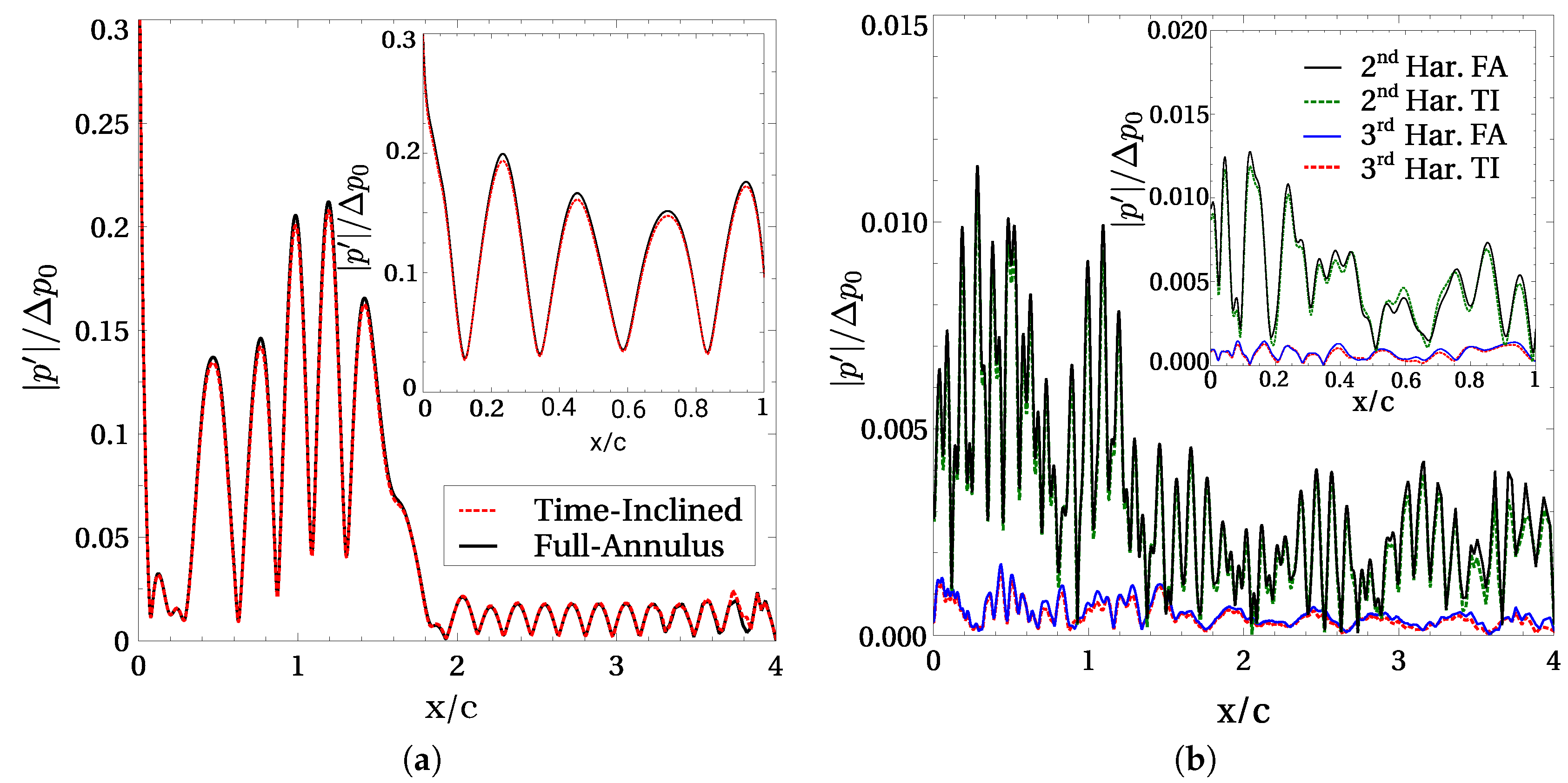
The same configuration was computed retaining the viscous terms. The Reynolds number based on the flat plate chord is $R{e}_c=1.1\times {10}^5$. The first observation is that the unsteady pressure fields created due to the interaction of the wake with the plate leading edge are different (see Figure 4a). The moduli of the unsteady pressure patterns are alike, but it can be observed that close to the plate, there is a short-wavelength oscillation caused by vortex shedding in the leading-edge region. The same behaviour can be observed in the first harmonic of the unsteady pressure distribution on the plate as well (Figure 4b). The comparison between the full-domain and time-inclined method is displayed in Figure 4b, in addition to a single-passage approximation that will be addressed in a following section. It can be noticed that although time-inclined and the directly periodic domain curves are alike, the agreement is not as good as that in the inviscid case. However, at the front and rear of the plate, the matching is good.

The root cause of the error is that a direct relationship between the transformed and the conservative variables, $\mathbf{U}=ϝ\left(\mathbf{Q}\right)$, does not exist for the Navier–Stokes equations, and therefore, the resulting set of equations is approximated. The problem is exacerbated in this case due to the high-frequency separation in the flat plate leading edge that sheds small vortices that are convected along the plate.

Figure 5 sketches the physics of the flow past a flat plate subject to incoming disturbances. Three regions of unsteadiness can be distinguished. Firstly, the plate passage contains wakes which are essentially undisturbed by the plates. Secondly, the plate has an unsteady boundary layer. In this case, the wall flow is affected by a separation in the leading edge that triggers the convection of small high-frequency vortices along the plate [29]. Finally, the plate trailing edge gives rise to a Karman vortex street that propagates and dissipates downstream. The impact of the TI transformation is different in the three regions. The frequency of the vortices created by the leading-edge separation is significantly higher than that of the incoming perturbation. The errors of the TI transformation are correspondingly higher too. High-frequency vortices propagating at nearly the free-stream velocity in a region dominated by the viscosity constitutes the most challenging case for the TI method.

The following subsections will show that the impact of the TI transformation on an LPT airfoil is much smaller than it is in this case. The main reason for the different behaviour of the TI method on the T106A airfoil is that well-designed LPT airfoils do not present leading-edge separation due to the favourable pressure gradient downstream of the leading edge.

3.1.3. Low Reynolds Number Case

The same case described in the previous subsection was simulated at a much lower Reynolds number ($Re$ = 10,000) to elucidate the origin of the discrepancies between the TI and the full-annulus solution. The grid was kept constant to increase the resolution and reduce the uncertainty associated with the different numerics of both methods. However, since the Reynolds number is lower than that in the previous case, the expected relative contribution of the nonphysical terms is higher.

Figure 6 displays the first harmonic of the unsteady pressure modulus along the passage’s midplane nondimensionalised with the total pressure perturbation imposed at the inlet, $\Delta p_0$. It can be observed that the matching between the TI and the full-annulus solution is nearly perfect. The highest unsteady pressure is located in the plate region. Downstream of the plate, for $x\ge 2c$, the unsteady pressure is much smaller, but the matching between both solutions is still good. The differences on the plate surface are hardly visible in the Figure 6 inset.

Figure 7a displays the evolution of the mean velocity profiles along the flat plate computed using the single-passage TI method and the equivalent multipassage domain with direct periodicity. First, it can be noticed that the matching between both approaches is nearly perfect. Except for that of the leading edge, all the remaining time-averaged profiles resemble the classical Blasius profiles at different $R{e}_x$. The boundary layer thickness is about 10% of the pitch at the plate exit, and therefore some blockage from the BL can be appreciated in the free-stream velocity.

The modulus of the first harmonic of the stream-wise velocity nondimensionalised with the exit isentropic velocity is shown in Figure 7b. The first harmonic of the perturbation velocity in the middle of the passage is about 2%. All the profiles exhibit extrema inside and outside of the boundary layer that are well-reproduced with the TI method. This result is consistent with the conclusions derived about the validity of the TI for unsteady laminar boundary layers. In this case, the boundary layer Strouhal number is $S{t}_{BL}=S{t}_{f}R{e}_c^{-1/2}$$\sim 40\times 10,{000}^{-1/2}/2\pi \sim 0.1$. The second and third harmonics of the problem are reproduced with the same level of accuracy as in Figure 6b, but they are not reproduced here for brevity.

A key aspect to match the results obtained by the TI and the full-annulus simulations is reproducing the wake mixing losses. If the wake mixing is mispredicted, then even the free-stream velocity can be mismatched, spoiling the whole comparison. The reduced frequency associated with the trailing-edge vortex shedding is fairly constant with the Reynolds number and typically is $S{t}_{TE}\simeq 0.2$. The Karman vortex street generated behind a 2D flat plate contains larger structures than does the three-dimensional wake behind an airfoil. As a consequence, this case is considered more demanding than a 3D wake.

Figure 8 displays the stream-wise evolution of the static pressure along a straight line of the computational domain with an offset of 50% of the pitch with respect to the plate. The matching between the TI and FA solution is very high until slightly after the trailing edge ($x/c=1.5$), where high vortices develop, fostering mixing. Differences can be appreciated downstream of this point, being the impact of the TI approach to this slightly delayed mixing.

Figure 9a compares the stream-wise evolution of the time-averaged total pressure profile downstream of the trailing edge computed using the TI (empty symbols), and the FA (filled symbols) approaches. The total pressure profiles match perfectly just downstream of the trailing edge ($(x-x_{te})/c=0$), indicating that up to this point, both approaches yield essentially the same solution. However, the downstream evolution diverges. It can be appreciated at $(x-x_{te})/c=0.33$ that the TI solution is less mixed than is the FA solution, i.e., its wake is deeper than that of the FA solution. Further downstream, where the wake is more mixed, the matching is recovered. Interestingly, the wake is not symmetric due the different degrees of unsteadiness created by the wake passing in the upper and lower sides of the plate. The pitch-wise area average of the profiles in Figure 9a can be seen in Figure 9b, which also shows their downstream evolution. The matching between the TI and FA approaches is good near the trailing edge, diverges downstream, and is recovered when the wake is nearly completely mixed.

Figure 10 displays a close-up of the 2D wake created downstream the flat plate by the TI and the FA approaches. One chord downstream of the trailing edge, the dissipation becomes very effective and the two solutions begin to diverge.

It is remarkable that even in this extreme case of high-frequency and a low Reynolds number leading to the presence of many wakes in the passage and thick boundary layers, $\delta /c\simeq 10\%$, the TI approach performs so well.

3.2. T106A LPT Linear Cascade

The T106A airfoil [28] was chosen to test the time-inclined method in a realistic configuration. The isentropic exit Mach number, $M_{2,is}=0.39$, the rotor Mach number, $M_r=0.52$, and the ratio between the rotor and the stator pitch, $P_r/P_s=15/6$, are the same as those in the flat-plate case. The Reynolds number based on the chord and the exit velocity is $R{e}_c=1.1\times {10}^5$. A sinusoidal perturbation of 2.5% of the total inlet pressure is imposed at the inflow. The computational domain is discretized using a hybrid grid of fourth-order triangles and quads. 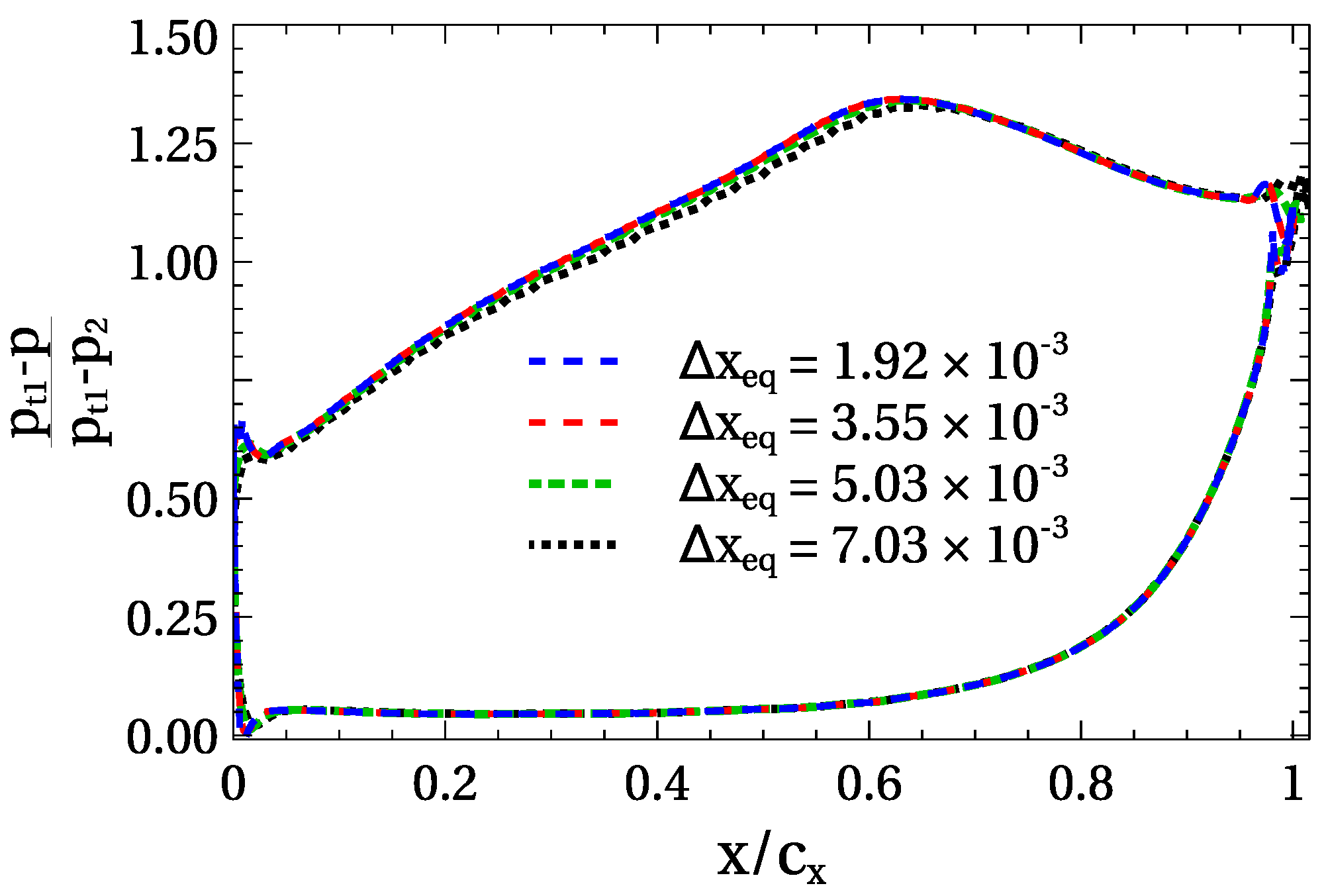The equivalent second-order mesh (See Figure 11) consists of 150 points on the airfoil and eight quad layers to account for the boundary layer region, totalling 7600 triangular cells and 3200 quad cells per passage. As in the flat-plate cascade case, the meshes of all the passages of the full-annulus cases are identical and equal to that of the time-inclined case. The fourth-order mesh has 16 degrees of freedom (DOF) per quad and 10 DOF per triangle. Although the focus of this work is to compare the TI and FA approaches and not to achieve the highest level of accuracy in the resolution of the physical phenomena, a grid independence analysis was conducted to choose the adequate mesh resolution. The results of this analysis can be found in Appendix A.

Figure 11 plots the first harmonic of the entropy to give an overall idea of the unsteady flowfield. It can be observed how the incoming wakes propagate undistorted through the inlet uniform field and then are distorted by the mean flow within the passage. A slight separation can be observed in the rear part of the suction side. The separation region is very small due to the highly reduced frequency of the incoming wakes ($k=\omega c/v_{2,is}=26.4$) that tend to suppress the steady separation. Qualitatively, this phenomenon is as described by Bolinches et al. [2] but in a much finer and three-dimensional grid.

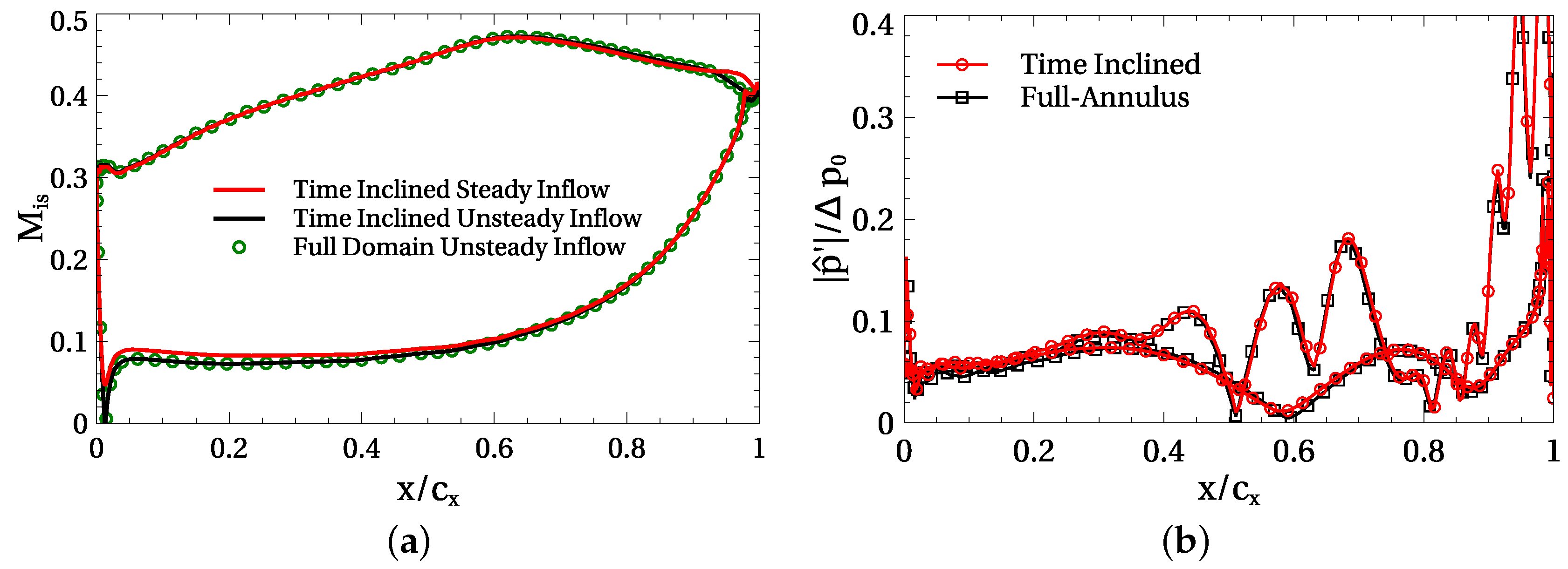
Figure 12a displays the mean isentropic Mach number distribution obtained via a viscous full-annulus analysis (6 passages) and the time-inclined method. It can be noticed that the matching between both is nearly perfect. The separation point, located at about 90% of the axial chord, is hardly visible. The case with the steady inflow (solid red line) exhibits a longer bubble that reattaches closer to the trailing-edge than to the unsteady inflow. Moreover, the pressure side is slightly different.

Figure 12b shows the distribution of the first harmonic of the unsteady pressure on the airfoil. The highest level of unsteadiness is located in the rear part of the suction side, where a closed and thin recirculating bubble can be seen. The shedding of this bubble gives rise to high unsteadiness. The second observation is that the agreement between the time-inclined approach and the full-domain simulation is very high. This degree of matching is the same for all the variables.

A comparison between the directly periodic and single-passage simulations is shown in Figure 4 and Figure 13. There were two single-passage simulations. The first was performed with the TI method matching the blade count and reduced frequency of the actual full-annulus case. The second employed the baseline code approximating a pitch ratio between the rotor and stator of three instead of using the exact $P_r/P_s$ = 15/6, and decreasing the velocity of the rotor to match the reduced frequency of the original problem.

Figure 4 compares the modulus of the first harmonic of the unsteady pressure obtained by the three methods in the flat-plate cascade. The agreement between the TI method and the full-annulus solution is better than that found for the approximate blade count. This is especially true for the areas close to the leading and trailing edges. The same observation can be made for the T106A cascade in the inviscid simulations, as shown in Figure 13, where the TI method matches the full-annulus solution very well, but the single-passage approximation grossly mispredicts the fundamental harmonic of the unsteady pressure.

Finally, Figure 14 shows a snapshot of the first harmonic of the unsteady pressure. The case is equivalent to having 15 stators in front of 6 rotors. A cutoff potential perturbation is clearly seen at the inlet. The suction side exhibits a strong unsteadiness caused by a local separation. This unsteadiness is synchronized with the inlet perturbation. This local unsteadiness is also captured with the time-inclined method.

3.3. Computational Cost Considerations

The computational cost per time step and point of the TI and baseline time-marching methods are essentially the same. In practice, only one additional operation is required per time step and solution point for time-inclining, which consists of transforming back the inclined variables $\mathit{Q}$ to the conservative variables $\mathit{U}$. This operation allows for the computation of the fluxes since they are a function of $\mathit{U}$, while the time-marching is performed on $\mathit{Q}$. However, the cost of this operation is negligible, especially for GPU architectures.

The impact on the maximum time step due to numerical stability constraints of the TI approach is simple to analyse and depends on the inclination parameter $\lambda$. However, even for the high inclination parameter chosen in the presented test cases, the TI simulations were carried out with the same time step as the full-annulus cases without numerical stability problems.

Finally, the computational cost reduction associated with reducing the number of passages is straightforward. In the cases presented in this work, the periodicity of the problem required a minimum of two passages in the full domain. Since the transformed cases were reduced to a single passage, the computational cost was halved. However, for realistic cases, the cost reduction is more significant.

Concerning computational cost, the most challenging part of quantifying its effect on the reduction obtained by the TI method is the convergence time to a periodically or a statistically converged state. The convergence time of the single-passage method is only sometimes well-understood, and small practical details of the implementation often hinder it [14,15]. Most rotor/stator simulations do not show a proper unsteady convergence analysis and, if any, it is restricted to monitoring the key engineering figures of merit of the problem.

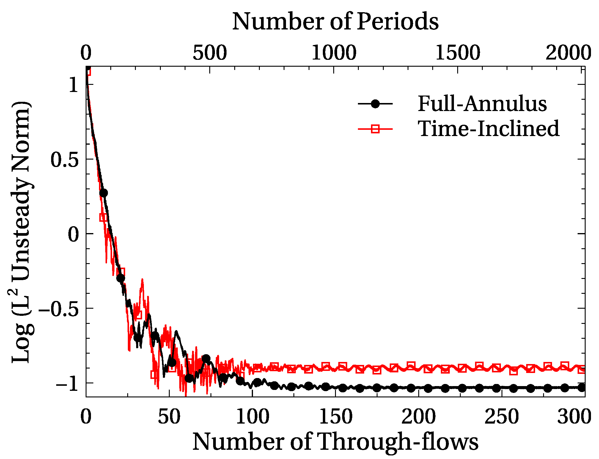
Figure 15 displays the unsteady norm $L^2$ of the FA analysis with direct periodicity and the TI method, where $L^2$ is defined as

$$L^2=\frac{1}{TS}\sqrt{{\displaystyle \underset{S}{\int }ds\underset{t_0}{\overset{t_0+T}{\int }}{\left\{\frac{p\left(t\right)-p(t-T)}{p(t-T)}\right\}}^2}}$$

(25)

where S is the airfoil surface. It can be noticed that the convergence rates of both approaches are similar, but they stall at a slightly different level. It is essential to recall that the final solution is not purely periodic since there are flow instabilities with frequencies different from the fundamental one. If these nonsynchronous frequencies dominate, then the chosen unsteady norm says very little about the final converged state. It can be noticed that the final state is reached in about 100-plate through-flow times, where the residence time is defined as $t_r=c/v_{2,is.}$ The total length of the computational domain is 4c. Since the convergence time is controlled by the total size of the computational domain, it can be stated that the solution converges in about 25 computational domain through-flow times, both in the TI and the full-annulus cases. The main conclusion is that the TI method does not degrade the convergence to the final state.

The physical convergence time of harmonically forced flows depends on the number of periods, $t_{con}\propto f^{-1}$, for low reduced frequency excitations or the number of through-flow times for high reduced frequency excitations, $t_{con}\propto t_r=c/v_c$. The required level of convergence depends on the amplitude of the highest harmonic resolved in the simulation. It can be anticipated that without a high level of convergence, it is impossible to match the third harmonic of the unsteady pressure shown in Figure 3 or Figure 6b, whose amplitude is a small fraction of the inlet total pressure (about ${10}^{-4}{p}_0$). It can be safely stated that the confidence in the level of convergence of the cases shown in this work is high.

A thorough description of the computational benefit of the TI method is postponed for a paper dedicated to this subject. However, if it is assumed that the convergence rate to the final state of both approaches is the same (see Figure 15) and the added time computational time per iteration is deemed negligible, then the cost reduction is proportional to the decrease in the size of the computational domain.

To provide an example, the low Reynolds ($R{e}_c={10}^4$) flat-plate case was run in a single NVIDIA GeForce GTX 1080Ti GPU for about 5160 and 9208 min using the time-inclined and the full-annulus approaches, respectively, yielding a speed-up factor of around 1.78.

4. Discussion

The time-inclined method was implemented in a high-order flux-reconstruction method for the first time and was applied to account for dissimilar gaps in rotor/stator interaction problems. The objective of this work is to reduce the computational time with a minimal loss in the fidelity of the problem. Results for two linear cascades and two different Reynolds numbers have been presented.

A linear cascade of flat plates was subject to a sinusoidal gust of total pressure. The inviscid results compare very well to those of the full-annulus simulations as expected since the TI transformation was exact for the inviscid cases. The matching of the low Reynolds number viscous case ($Re={10}^4$) was nearly perfect as well, whereas that of the high Reynolds number case ($Re={10}^5$) was not. It can be argued that the root cause of the differences in the latter is associated with the separation of the flow in the flat-plate leading edge that gives rise to a high-frequency oscillation that propagates downstream along the plate. The high-frequency nature of the problem magnifies the errors and the intrinsic inaccuracies of the TI method in dealing with unsteady viscous flows. However, this problem is deemed irrelevant in practical applications.

A cascade of T106A airfoils with similar inlet conditions to the flat plate case was simulated at representative Reynolds numbers. The matching, in this case, was as good as that of the flat plate at low Reynolds numbers. The agreement of the mean solution and the first harmonic with the full-domain simulation was very good.

5. Conclusions

This is the first time, in the authors’ opinion, that the limitations of the TI method for viscous flows have been explored in general and particularly in the context of a high-order flux-reconstruction method, making the discussion more relevant. It can be concluded that the technique can be further pursued and applied to scale-resolving simulations. Theoretical arguments have been presented that show that the TI method can be applied to LES or under-resolved direct numerical simulations even though the wavelengths of the unsteadiness are very short and the impact of viscous terms has not been assessed yet in eddy-resolving simulations. The test cases were designed to explore the limits of the TI approach, and hence the results are considered satisfactory for many problems of industrial interest, with most of the conclusions being applicable to 3D turbulent cases.

References

1. Bolinches-Gisbert, M.; Cadrecha-Robles, D.; Corral, R.; Gisbert, F. Prediction of Reynolds Number Effects on Low-Pressure Turbines Using a High-Order ILES Method. J. Turbomach. 2020, 142, 031002. [Google Scholar] [CrossRef]
2. Bolinches-Gisbert, M.; Cadrecha-Robles, D.; Corral, R.; Gisbert, F. Numerical and Experimental Investigation of the Reynolds Number and Reduced Frequency Effects on Low-Pressure Turbine Airfoils. J. Turbomach. 2021, 143, 021004. [Google Scholar] [CrossRef]
3. Michelassi, V.; Chen, L.W.; Pichler, R.; Sandberg, R.D. Compressible Direct Numerical Simulation of Low-Pressure Turbines–Part II: Effect of Inflow Disturbances. J. Turbomach. 2015, 137, 071005. [Google Scholar] [CrossRef]
4. Michelassi, V.; Chen, L.; Pichler, R.; Sandberg, R.; Bhaskaran, R. High-fidelity Simulations of Low-Pressure Turbines: Effect of Flow Coefficient and Reduced Frequency on Losses. J. Turbomach. 2016, 138, 111006. [Google Scholar] [CrossRef]
5. Pichler, R.; Michelassi, V.; Sandberg, R.; Ong, J. Highly Resolved Large Eddy Simulation Study of Gap Size Effect on Low-Pressure Turbine Stage. J. Turbomach. 2018, 140, 021003. [Google Scholar] [CrossRef]
6. Lewis, D.; Moreau, S.; Jacob, M.C.; Sanjosé, M. ACAT1 Fan Stage Broadband Noise Prediction Using Large-Eddy Simulation and Analytical Models. AIAA J. 2022, 60, 360–380. [Google Scholar] [CrossRef]
7. Polacsek, C.; Daroukh, M.; François, B.; Barrier, R. Zonal Detached Eddy Simulation of the Fan-Outlet Guide Vanes Stage of a Turbofan Engine: Part II—Broadband Noise Predictions. J. Turbomach. 2022, 144, 111005. [Google Scholar] [CrossRef]
8. Erdos, J.; Alzner, E.; McNally, W. Numerical Solution of Periodic Transonic Flow through a Fan Stage. AIAA J. 1977, 15, 1559–1568. [Google Scholar] [CrossRef]
9. Burgos, M.; Corral, R. Application of Phase-Lagged Boundary Conditions to Rotor/Stator Interaction. In Proceedings of the ASME Turbo Expo 2001: Power for Land, Sea, and Air, New Orleans, LA, USA, 4–7 June 2001; Volume 1, p. V001T03A088. [Google Scholar] [CrossRef]
10. Dewhurst, S.; He, L. Unsteady Flow Calculations through Turbomachinery Stages Using Single-Passage Domain with Shape-Correction Method. In Proceedings of the Ninth International Symposium on Unsteady Aeroedynamics, Aeroelasticity and Aeroacoustics; Ferrand, P., Aubert, S., Eds.; Presses Universitaires de Grenoble: Lyon, France, 2000; pp. 338–350. [Google Scholar]
11. Li, H.; He, L. Toward Intra-Row Gap Optimization for One and Half Stage Transonic Compressor. J. Turbomach. 2005, 127, 589–598. [Google Scholar] [CrossRef]
12. Mouret, G.; Gourdain, N.; Castillon, L. Adaptation of Phase-Lagged Boundary Conditions to Large Eddy Simulation in Turbomachinery Configurations. J. Turbomach. 2016, 138, 041003. [Google Scholar] [CrossRef]
13. Montero-Villar, G.; Lindblad, D.; Andersson, N. Investigation of Phase-Lagged Boundary Conditions for Turbulence Resolving Turbomachinery Simulations. In Proceedings of the AIAA AVIATION 2020 FORUM, Online, 15–19 June 2020. Number AIAA 2020-2982. [Google Scholar] [CrossRef]
14. Biesinger, T.; Cornelius, C.; Rube, C.; Braune, A.; Campregher, R.; Godin, P.G.; Schmid, G.; Zori, L. Unsteady CFD Methods in a Commercial Solver for Turbomachinery Applications. In Proceedings of the ASME Turbo Expo 2010: Power for Land, Sea, and Air, Glasgow, UK, 14–18 June 2010; Volume 7, pp. 2441–2452. [Google Scholar] [CrossRef]
15. Giovannini, M.; Marconcini, M.; Arnone, A.; Bertini, F. Evaluation of Unsteady Computational Fluid Dynamics Models Applied to the Analysis of a Transonic High-Pressure Turbine Stage. Proc. Inst. Mech. Eng. Part A J. Power Energy 2014, 228, 813–824. [Google Scholar] [CrossRef]
16. Giles, M.B. Stator/Rotor Interaction in a Transonic Turbine. J. Propuls. Power 1990, 6, 621–627. [Google Scholar] [CrossRef]
17. Giles, M. UNSFLO: A Numerical Method for Unsteady Inviscid Flow in Turbomachinery; Technical Report; Gas Turbine Laboratory, Massachusetts Institute of Technology: Cambridge, MA, USA, 1988. [Google Scholar]
18. Cornelius, C.; Biesinger, T.; Zori, L.; Campregher, R.; Galpin, P.; Braune, A. Efficient Time Resolved Multistage CFD Analysis Applied to Axial Compressors. In Proceedings of the ASME Turbo Expo 2014: Turbine Technical Conference and Exposition, Dusseldorf, Germany, 16–20 June 2014; Volume 2D: Turbomachinery. p. V02DT44A035. [Google Scholar] [CrossRef]
19. Moura, R.; Sherwin, S.; Peiró, J. Linear Dispersion–Diffusion Analysis and its Application to Under-Resolved Turbulence Simulations Using Discontinuous Galerkin Spectral/hp Methods. J. Comput. Phys. 2015, 298, 695–710. [Google Scholar] [CrossRef]
20. Gisbert, F.; Bolinches-Gisbert, M.; Pueblas, J.; Corral, R. Efficient Implementation of Flux Reconstruction Schemes for the Simulation of Compressible Viscous Flows on Graphics Processing Unigs. In Proceedings of the Tenth International Conference on Computational Fluid Dynamics, ICCFD10-307, Barcelona, Spain, 9–13 July 2018. Number ICCFD10-307. [Google Scholar]
21. Corral, R.; Gisbert, F.; Pueblas, J. Execution of a Parallel Edge-Based-Navier-Stokes Solver on Commodity Graphics Units. Int. J. Comput. Fluid Dyn. 2017, 31, 93–108. [Google Scholar] [CrossRef]
22. Huynh, H.T. A Flux Reconstruction Approach to High-Order Schemes Including Discontinuous Galerkin Methods. In Proceedings of the 18th AIAA Computational Fluid Dynamics Conference, AIAA 2007-4079, Miami, FL, USA, 25–28 June 2007. [Google Scholar] [CrossRef]
23. Wang, Z.; Gao, H. A Unifying Lifting Collocation Penalty Formulation Including the Discontinuous Galerkin, Spectral Volume/Difference Methods for Conservation Laws on Mixed Grids. J. Comput. Phys. 2009, 228, 8161–8186. [Google Scholar] [CrossRef]
24. Giles, M. UNSFLO: A Numerical Method for the Calculation of Unsteady Flow in Turbomachinery; Technical Report; Gas Turbine Laboratory, Massachusetts Institute of Technology: Cambridge, MA, USA, 1991. [Google Scholar]
25. Batchelor, G.; Proudman, I. The effect of rapid distortion of a fluid in turbulent motion. Q. J. Mech. Appl. Math. 1954, 7, 83–103. [Google Scholar] [CrossRef]
26. Blázquez-Navarro, R.; Corral, R. Validation of Broadband Noise Prediction Methodology Based on Linearised Navier-Stokes Analyses. J. Turbomach. 2023, 1–25. [Google Scholar] [CrossRef]
27. Blázquez-Navarro, R.; Corral, R. Prediction of fan acoustic blockage on fan/outlet guide vane broadband interaction noise using frequency domain linearised Navier–Stokes solvers. J. Sound Vib. 2021, 500, 116033. [Google Scholar] [CrossRef]
28. Hoheisel, H.; Kiock, R.; Lichtfuss, H.; Fottner, L. Influence of Free-Stream Turbulence and Blade Pressure Gradient on Boundary Layer and Loss Behavior of Turbine Cascades. J. Turbomach. 1987, 109, 210–219. [Google Scholar] [CrossRef]
29. Lin, N.; Reed, H.; Saric, W. Effect of Leading-Edge Geometry on Boundary-Layer Receptivity to Freestream Sound. In Instability, Transition, and Turbulence; ICASE NASA LaRC Series; Springer: New York, NY, USA, 1992; pp. 421–440. [Google Scholar]
Figure 1. Nomenclature and illustration of a rotor/stator problem with dissimilar gaps.
Aerospace 10 00475 g001
Figure 2. Schematic of the flat plate cascade with inlet perturbations.
Aerospace 10 00475 g002
Figure 3. Modulus of the first (left axis), second, and third (right axis) harmonics of the unsteady pressure on the plate (inviscid case).
Aerospace 10 00475 g003
Figure 4. (a) Modulus of the first harmonic of the pressure in the inviscid and viscous cases and (b) modulus of the first harmonic of the pressure on the lower side of the plate for the full-annulus (black), time-inclined (red), and single-passage (blue) methodologies.
Aerospace 10 00475 g004
Figure 5. Physics of the viscous flow past a cascade of flat plates at high Reynolds numbers sketched by a snapshot of the entropy.
Aerospace 10 00475 g005
Figure 6. First (a), second, and third (b) harmonics of the unsteady pressure along the passage midline and along a plate (inset) at R e = 10,000.
Aerospace 10 00475 g006
Figure 7. (a) Time-averaged and (b) first harmonic velocity profiles in the flat plate boundary layer. Time-inclined (dotted lines) vs. full-annulus approach (solid lines).
Aerospace 10 00475 g007
Figure 8. Stream-wise evolution of the time-averaged static pressure along a straight line of the flat plate channel with an offset of 50% of the plate ( R e = 10,000).
Aerospace 10 00475 g008
Figure 9. (a) Stream-wise evolution of the time-averaged total pressure profiles in the flat-plate wake at R e = 10,000 and (b) Stream-wise evolution of the azimuthally and time-averaged total pressure profiles. The horizontal axis measured from the trailing edge is denoted as z = x x T E .
Aerospace 10 00475 g009
Figure 10. Close-up of a snapshot of the entropy isolines for R e = 10,000. Top: Time inclined. Bottom: Full annulus.
Aerospace 10 00475 g010
Figure 11. Second-order mesh detail and real part of the first harmonic of the entropy for the T106A airfoil at R e c = 1.1 × 10 5 .
Aerospace 10 00475 g011
Figure 12. (a) Comparison of the mean isentropic Mach number distribution and (b) the first harmonic of the unsteady pressure for the T106A between the full-annulus analysis and the time-inclined method.
Aerospace 10 00475 g012
Figure 13. First harmonic of the unsteady pressure for the inviscid T106A linear cascade. Comparison between the full-annulus (black), time-inclined (red), and single-passage (blue) methodologies.
Aerospace 10 00475 g013
Figure 14. Snapshot of the of the real part of the first harmonic of the static pressure of a viscous solution for the T106A airfoils.
Aerospace 10 00475 g014
Figure 15. Convergence history of a flat-plate cascade as a function of the number of inlet disturbance periods and through-flow times ( t r = c / v 2 , i s ).
Aerospace 10 00475 g015
Disclaimer/Publisher’s Note: The statements, opinions and data contained in all publications are solely those of the individual author(s) and contributor(s) and not of MDPI and/or the editor(s). MDPI and/or the editor(s) disclaim responsibility for any injury to people or property resulting from any ideas, methods, instructions or products referred to in the content.