
Classification of Systems and Maintenance Models


1
Department of Electronics, Robotics, Monitoring and IoT Technologies, National Aviation University, 03058 Kyiv, Ukraine
2
PDP Engineering Section, The Private Department of the President of the United Arab Emirates, Abu Dhabi 000372, United Arab Emirates
*
Author to whom correspondence should be addressed.
Aerospace 2023, 10(5), 456; https://doi.org/10.3390/aerospace10050456
Submission received: 15 March 2023
/
Revised: 8 May 2023
/
Accepted: 12 May 2023
/
Published: 15 May 2023
(This article belongs to the Special Issue Predictive Maintenance for Complex Systems—from Sensor Measurements to Prognostics to Maintenance Planning)
Abstract
:Maintenance is an essential part of long-term overall equipment effectiveness. Therefore, it is essential to evaluate maintenance policies’ effectiveness in addition to planning them. This study provides a classification of technical systems for selecting maintenance effectiveness indicators and a classification of maintenance models for calculating these indicators. We classified the systems according to signs, such as system maintainability, failure consequences, economic assessment of the failure consequences, and temporary mode of system use. The classification of systems makes it possible to identify 13 subgroups of systems with different indicators of maintenance effectiveness, such as achieved availability, inherent availability, and average maintenance costs per unit of time. When classifying maintenance models, we used signs such as the system structure in terms of reliability, type of inspection, degree of unit restoration, and external manifestations of failure. We identified one hundred and sixty-eight subgroups of maintenance models that differed in their values for specified signs. To illustrate the proposed classification of maintenance models, we derived mathematical equations to calculate all considered effectiveness indicators for one subgroup of models related to condition-based maintenance. Mathematical models have been developed for the case of arbitrary time-to-failure law and imperfect inspection. We show that the use of condition-based maintenance significantly increases availability and reduces the number of inspections by more than half compared with corrective maintenance.
1. Introduction
According to the British standard BS EN 13306:2017, “Maintenance is a combination of all technical, administrative, and managerial actions during the life cycle of an item intended to retain it in, or restore it to, a state in which it can perform the required function [1].” Numerous maintenance types and techniques, such as condition-based maintenance (CBM) [2,3], predictive maintenance [4], prescriptive maintenance [5], remote maintenance [6,7], preventive maintenance [8,9], and e-maintenance [10,11] have been developed in recent decades. Owners of various pieces of equipment face three key maintenance challenges: lowering maintenance costs, increasing availability or operational reliability, and selecting the most effective techniques to improve operational characteristics. The estimated maintenance costs range from 15% to 70% of the cost of items sold [12]. A significant part of the losses is due to unplanned downtime. According to [13], industrial manufacturers incur an estimated USD 50 billion in annual losses owing to unplanned downtime and equipment failure accounts for 42% of this unplanned downtime. Therefore, it is crucial to assess the effectiveness of maintenance policies in addition to developing them.
In the following, we discuss the concept of a maintenance and repair system (MRS). We define MRS as a set of tools, maintenance, and repair documentation, and performers necessary to maintain and restore the object of maintenance (OM). The difference between maintenance and repair is that maintenance is conducted to prevent unexpected equipment downtime, whereas repair is conducted following downtime to restore the OM operable state and reduce losses. Under MRS effectiveness, we refer to a set of properties that characterize the ratio between the costs of resources (material, time, or labor) to maintain and restore the health of the OM and the effect achieved. The effectiveness of MRS depends on the reliability, maintainability, and durability of the OM as well as the trustworthiness of inspections or condition monitoring. The quantitative characteristics of various MRS properties are indicators of the reliability, maintainability, durability, and trustworthiness of the inspections. For example, indicators of inspection trustworthiness quantitatively characterize the properties of the inspection tool, which is a subsystem in the MRS, to objectively display the actual condition of the OM based on the inspection results.
Currently, technical and technical-economic indicators are used to quantify maintenance effectiveness. Technical indicators include the achieved availability, inherent availability, mission availability, and operational reliability. Technical-economic indicators include the long-run average profit per unit time and long-run average cost per unit time.
Choosing maintenance effectiveness indicators of a system requires identifying the key features that distinguish it from others. Therefore, for the proper selection of MRS effectiveness indicators, the development of a technical system classification is required according to signs that consider the unique features of their design, intended use, and operating conditions.
After selecting the MRS effectiveness indicators, a maintenance model should be developed or chosen for the calculation. This model should reflect the features of the structural construction of the system in terms of reliability, the presence of external manifestations of failure, and the main signs of maintenance operations. Since any MRS necessarily includes an inspection subsystem and a recovery subsystem, the maintenance model should consider the characteristics of operations, including inspection and repair. The efficiency of using a system for its intended purpose depends on the type of inspection. Therefore, the maintenance model should consider the type of inspection and the degree of system repair.
Based on the literature review in Section 2, the following findings can be drawn:
- (1)
- Performance indicators are considered at three levels of maintenance control: strategic, tactical, and operational.
- (2)
- An analysis of the published studies revealed that diverse types of maintenance performance indicators exist in the literature for each level of maintenance control.
- (3)
- At the operational stage, the most frequently used maintenance indicators are instantaneous availability, steady-state availability, average availability, inherent availability, mission availability, operational reliability, long-run average profit per unit time, long-run average cost per unit time, and average lifetime maintenance costs.
- (4)
- To date, several classifications of maintenance performance indicators have been developed, including, for example, such categories of indicators as equipment-related, maintenance task-related, cost-related, and so on. However, the signs by which indicators should be selected in each group for systems of various purposes have not been indicated. Since a formalized approach to selecting the indicators has not been developed, users are forced to subjectively choose suitable indicators for their circumstances from a set of known indicators.
- (5)
- The same effectiveness indicators were used for diverse types of maintenance, including preventive, corrective, condition-based, predictive, and prescriptive maintenance. Simultaneously, there is no formal classification of maintenance models that allows an appropriate model to be objectively chosen according to certain features.
- (6)
- There is no formalized approach to the classification of systems for selecting maintenance effectiveness indicators and for the classification of the maintenance models necessary to calculate the selected indicators.
- (7)
- In the existing preventive, corrective, condition-based, and predictive maintenance models, it is assumed that failures are detected using periodic (or sequential) inspections and/or continuous condition monitoring.
- (8)
- Prescriptive maintenance uses condition monitoring and artificial intelligence to track a larger range of data and predict when maintenance is necessary in real-time.
In this study, we propose a classification of technical systems that allows us to select maintenance effectiveness indicators depending on signs such as system maintainability, failure consequences, an economic assessment of the failure consequences, and a temporary mode of system use. This classification makes it possible to identify 13 subgroups of indicators, including most of the known indices and some new ones.
The study also proposes a classification of maintenance models to calculate each maintenance effectiveness indicator. The developed classification allows the selection of a maintenance model depending on features such as the system structure in terms of reliability, type of inspection, degree of the system’s restoration, and external manifestations of failure. This classification makes it possible to identify one hundred and sixty-eight subgroups of the maintenance models.
We illustrate how to determine the maintenance effectiveness indicators for a subgroup of maintenance models, which assume that the system has a single-component structure, that the type of inspection is similar to CBM, that the perfect repair is used, and that only hidden failures occur in the system. We developed mathematical maintenance models for the case of an arbitrary distribution of time-to-failure and multiple imperfect inspections, where the probabilities of correct and incorrect decisions depend on the time of inspection and failure occurrence. A numerical example illustrates the determination of the optimal number of inspections for a particular stochastic degradation process in condition-based and corrective maintenance.
The remainder of this article is organized as follows: Section 2 provides a review of the classification of maintenance effectiveness indicators and maintenance models. The classification of technical systems for selecting maintenance effectiveness indicators is discussed in Section 3. Section 4 presents the classification of the maintenance models. Section 5 develops the condition-based maintenance model and provides formulas for calculating maintenance effectiveness indicators. In Section 6, an example of deterioration process modeling is considered. The results are outlined in Section 7, followed by a discussion in Section 8. Section 9 presents the conclusions and potential future work. Abbreviations and references are provided at the end of this article.
2. Literature Review
Most studies on the evaluation of maintenance indicators deal with performance metrics that fall into two groups: those that show how maintenance affects a system’s overall performance, and those that address a system’s operational reliability and availability. The long-run average profit per unit time of using the system is representative of the first group of indicators. Well-known representatives of the second group are achieved and inherent availability.
The literature on the classification of maintenance effectiveness or performance indicators is abundant. Reviews of the classification of maintenance performance indicators can be found in [14,15,16]. In summary, the study [14] concludes that successful maintenance performance indicators should concentrate on assessing total maintenance effectiveness [17]. Seven categories of maintenance performance indicators that measure the overall maintenance effectiveness were included in this study [18]. Cost-, equipment-, and maintenance-task-related indicators are the most crucial. The study [15] examined the development of maintenance performance measures concerning the crucial maintenance organizational function and its resources, activities, and practices. According to a study [16], lagging measures, such as maintenance cost and safety performance, dominate the measurement of maintenance performance. Leading indicators such as maintenance work processes are used less frequently. The findings revealed no connection between the indicators employed and the maintenance goals pursued. The study in [19] used the original ELECTRE I, a multi-criteria decision-making method, to present a novel method for selecting maintenance key performance indicators. Following evaluations based on the key criteria, the suggested methodology generates a ranking of potential options. The study in [20] considered three levels of maintenance control: strategic, tactical, and operational. A set of maintenance performance indicators can be considered at each maintenance level. This study concentrates on maintenance performance indicators that support decisions at the operational level. The balanced scorecard is a different and comprehensive approach to measuring maintenance performance, as suggested in this study [21]. It is based on the idea that no single measure can accurately reflect the overall maintenance performance and that multiple measures must be used in conjunction.
Let us consider the published indicators of maintenance effectiveness used in the operational stage. The study in [22] used instantaneous and steady-state availability as maintenance effectiveness indicators. The best inspection and imperfect maintenance policy that reduces the average long-term cost rate is then obtained using availability models. The study in [23] considered an analytical model for the steady state and instantaneous availability of the system. The authors determined the best method to change the inspection interval to maximize the steady-state availability of the system. A study [24] considered steady-state availability as a critical metric for telecommunication services in which network functions are handled using software. To determine the lower confidence limit of the availability of complex control systems, the study [25] presented a new availability assessment approach based on the goal-oriented method. The study [26] looked at a continuously tested digital electronic system that could have one of three failures: revealed, unrevealed, or intermittent. A new maintenance model for determining inherent availability was proposed. A mathematical model to describe mission availability for a system with bounded cumulative downtime was proposed in [27]. The suggested approach simultaneously considers cumulative uptime and downtime as restrictions. The study [28] considered a mathematical model to compute the operational reliability of an avionic line-replaceable unit (LRU), the probability of LRU recovery, and the maintenance cost. In [29], the authors considered corrective maintenance policies for scheduled imperfect inspections. The maintenance effectiveness indicators are the average availability and long-run average cost per unit time. A study in [30] suggested a new CBM model that uses an energy efficiency indicator. The suggested approach encourages CBM optimization to consider both useful output performance and maintenance costs. The study in [31] focused on the analytical modeling of a condition-based inspection and replacement policy for a stochastically and continuously degrading single-unit system. The developed mathematical model allows for the evaluation of the effectiveness of the maintenance policy and minimizes the expected long-term maintenance cost per unit time. A CBM policy was developed in the study [32] for a two-component system with stochastic and economic dependencies. The long-term expected maintenance cost per unit time is an indicator of maintenance effectiveness. In [33], a mathematical model of preventive maintenance with imperfect continuous condition monitoring of wind turbine components was presented. The derived mathematical equations allow the calculation of both the average lifetime maintenance cost and expected maintenance cost per unit time. A study [34] proposed a comprehensive approach for the reliability modeling and maintenance planning of parallel repairable systems that suffer from hidden failures. This study aimed to reduce the expected maintenance cost per unit time by jointly determining the optimal inspection interval and maintenance thresholds. A study [35] established maintenance policies for a system under periodic inspections. Maintenance actions were performed for any failures that were found. Repair is imperfect. The expected variable cost rate is an indicator of maintenance effectiveness. A study [36] examined the problem of determining the optimal aircraft equipment maintenance intervals while minimizing maintenance costs and assuming an Erlang distribution of time between failures. The study in [37] focused on a technique for calculating the optimal threshold during the implementation of the condition-based maintenance of radio equipment. The minimum average operational costs served as the optimization criterion. The study in [38] examined the cost-effectiveness of applying CBM in manufacturing companies. The findings indicate that two potentially important benefits of CBM include lowering the probability of maximum damage to manufacturing machinery and of production losses, particularly in high production volumes. The study in [39] considered a sensory-updated predictive maintenance policy that forecasts and updates the residual life distribution of a simple manufacturing cell using degradation models and sensor information. The overall maintenance costs are then computed. By considering imperfect remaining useful life (RUL) prognostics based on condition monitoring data, [40] proposed a dynamic, predictive maintenance scheduling framework for a fleet of aircraft. This framework reduced the maintenance costs associated with engine failures to only 7.4% of the overall maintenance costs. A study [41] examined a production system that was regularly inspected. Manufacturing, inventory, lost sales, repair, inspection, and maintenance costs are all included in the expected cost function. The study [42] considered a strategic queuing model to examine how a maintenance service provider should allocate capacity and set prices in the face of imperfect IoT-based diagnostics, which continuously monitor various pieces of equipment using sensors. The study in [43] investigated two maintenance strategies for wind-turbine gearboxes using continuous temperature monitoring. The maintenance effectiveness indicator is the total expected cost per unit time. According to a numerical analysis of the presented models, the optimal imperfect preventive maintenance strategy was 46% more effective than the optimal renewal strategy. A study [44] proposed a technique for managing the maintenance of wind turbines using artificial intelligence approaches to reduce the overall cost. According to the study, the electrical system, gearbox, generator, and blades account for more than 80% of the risk factor and related downtime; as a result, they should be monitored and inspected more frequently than the others. The study in [45] created a big data analytics platform that lowers maintenance costs by optimizing the maintenance schedule through CBM optimization and increasing the accuracy of quantifying the RUL prediction uncertainty. The study [46] proposed a wind farm predictive maintenance approach that considered the economic dependency among subassemblies and component-level major and minor repairs. A simulation method was developed to assess maintenance costs. The study in [47] proposed a reinforcement learning method to explore optimal predictive maintenance policies that optimize production and maintenance costs. The study in [48] determined an optimal preventive maintenance schedule that was predicted based on the industry’s maximum availability of critical part manufacturing systems. A study [49] developed a highly accurate RUL prediction for machinery using sensor-monitoring data. The proposed approach provides a more accurate RUL prediction than existing data-driven prediction methods. The study in [50] built a distributed system with artificial intelligence assistance for applications in manufacturing plant-wide predictive maintenance based on sensors. The study in [51] considered a sensor deployment problem to minimize maintenance costs. The authors developed a maintenance cost model for IoT networks that considers thermal degradation and battery depletion. A study [52] proposed a maintenance model for protection systems with imperfect inspections. The conditional probabilities of correct and incorrect inspections are assumed to be constant. The maintenance effectiveness indicator was the expected cost per regeneration cycle. Studies [53,54] have shown that the probabilities of imperfect inspections at condition-based and predictive maintenance are functions of the degradation model parameters and strongly depend on time. In the study [55], the case of imperfect testing of the crack depth in a fighter wing was considered. The study showed that flight hours have a significant impact on the probabilities of a false positive and a false negative. The study in [56] analyzed six main components of intelligent predictive maintenance: (1) sensor and data acquisition, (2) signal pre-processing and feature extraction, (3) maintenance decision-making, (4) key performance indicators, (5) maintenance scheduling optimization, and (6) feedback control and compensation. The study [57] presented a new data-driven predictive maintenance approach that covers the full process, from using RUL prediction to making maintenance decisions. The maintenance cost per unit time was calculated. The study in [58] proposed probabilistic models for assessing mission success probability, system survival probability, expected number of inspections during the mission, and total estimated losses for a system subject to imperfect inspections. In the developed models, the probabilities of false positives and false negatives were time-independent.
The studies [59,60,61,62,63,64] considered the application of preventive, condition-based, and predictive maintenance techniques in the context of Industry 4.0. Among the novel maintenance approaches and techniques, special attention is given to the data-driven approach, conventional machine learning approaches, and machine prognostics for RUL estimation. Studies [65,66,67,68,69,70] introduced prescriptive maintenance techniques that may not only predict the condition of a machine in the future but also suggest proactively timed decisions for certain maintenance activities such as inspection, repair, and replacement. Studies [71,72,73,74,75,76] considered the use of knowledge-based approaches in predictive, condition-based, prescriptive, and preventive maintenance.
3. Classification of Systems
As noted in Section 1, the design of the system, its purpose, and its operating conditions affect the choice of MRS effectiveness indicators. To classify the systems, we characterized each of the listed generalized properties by using a minimum set of the most significant signs.
From a maintenance perspective, the design of a system is primarily characterized by its maintainability. According to [1], “maintainability is the ability of an item under given conditions of use, to be retained in, or restored to, a state in which it can perform a required function.” Items that can be repaired are compared with those that cannot be repaired because of planned obsolescence. The division of systems into repairable and non-repairable systems is associated with the possibility of restoring an operable state through repair, which is ensured during the development and manufacture of the system.
We should also note that sometimes the term “repairability” is used to characterize the ability of a system to be repaired. Maintainability and repairability are similar. The only distinction is that while repairability is limited to active repair time, maintainability is based on total downtime (which includes administrative time, active repair time, and logistic time). In addition, the term “maintainability” is standard [1], while the term “repairability” is not.
The concept of “purpose of the system” primarily relates to the functions it performs. However, this concept includes not only the list of functions performed but also the relative importance of these functions. These two circumstances can be characterized by qualitative and quantitative assessments of the events that occur owing to system failure, that is, the consequences of failure and the possibility of their quantitative assessment.
The evaluation of maintenance effectiveness is carried out using indicators that depend on the operating time of the system in a given mode of temporary use, which may be continuous or intermittent. That is why, as a sign of the classification that characterizes the mode of operation, we chose the temporary mode of using the system for its intended purpose.
Therefore, we classified systems according to the following criteria: maintainability, consequences of a failure, possibility of an economic assessment of the consequences of a failure, and temporary mode of system use.
To divide a set of system types into subsets according to the listed signs, it is necessary to select a classification system. Currently, the most common classification systems for information objects are hierarchical and faceted [77].
A hierarchical system is used when a subordination relationship is established between the classification signs used at levels i and (i + 1).
With a faceted classification system, we subdivide the initial set of objects into subsets by combining the values of the independent signs (facets).
As shown below, for the four signs under consideration, a subordination relation exists between all features. Therefore, it is necessary to apply a hierarchical classification system with ordinal registration of individual sign values.
We determined the values of the classification signs, established a connection between them, and divided the initial set of systems into disjointed subsets as follows.
First classification sign. A sign of system maintainability i (i = 1: the system is repairable; i = 2: the system is non-repairable).
When using “repairable”, we refer to the systems for which the repair is provided in the technical documentation.
Non-repairable systems will include systems whose performance cannot be restored owing to design features or whose restoration is not economically feasible. However, for non-repairable systems, maintenance may be provided, including condition monitoring and removal if necessary.
Therefore, in the first stage of the classification, the initial set of systems I0 is divided according to sign i into the class of repairable systems I1 and the class of non-repairable systems I2, that is,
moreover , where , , and are symbols denoting the union and intersection of subsets, and an empty subset, respectively.
Figure 1a illustrates the classification of systems by sign i.
Second classification sign. A sign of failure’s consequences j (j = 1: the fact that the system does not perform a safety-critical function assigned to it in a given volume, j = 2: the fact that the system does not perform a safety-critical function assigned to it in a given volume at an arbitrary moment of beginning the “operation mode,” j = 3: downtime of the system in a state of unrevealed failure when used as intended and downtime associated with scheduled maintenance and unscheduled repair; j = 4: downtime of the system in a state of unrevealed failure when used as intended, regardless of the downtime associated with scheduled maintenance; j = 5: downtime of the system in a state of unrevealed failure when used as intended and downtime associated with unscheduled system replacement).
When evaluating the consequences of a failure, the sign value of j = 1 corresponds to the case in which the consequences affect safety. According to the European Standard ECSS-S-ST-00-01C––Glossary of Terms [78], “a safety-critical function is the function that, if lost or degraded, or as a result of incorrect or inadvertent operation, can result in catastrophic or critical consequences.” When j = 2, the system can be either in standby mode or operation mode, and when it is in operation mode, it does not perform a safety-critical function. In the standby mode, the system is accessible for inspection and repair. The system must operate without failure for a predetermined time in the operating mode, where failure affects safety. Maintenance and inspection were not performed in the operating mode.
The sign value j = 3 corresponds to the case when material damage due to a failure is caused by both the system’s downtime in a state of unrevealed failure during operation and by the downtime due to the restoration.
The sign value j = 4 corresponds to the case in which the material damage owing to a failure is much greater than the losses caused by the system downtime. In this case, as a rule, the system downtime owing to restoration work does not lead to substantial material loss. If it is impossible to estimate material losses due to system failure, the value j = 4 corresponds to the case in which either scheduled maintenance or restoration of the system, or both, can be carried out during time intervals when the system is not used.
The sign value j = 5 corresponds to the operation of a non-repairable system, the consequences of which do not affect safety.
The sign values j = 2, 3, and 4 correspond to the cases of operation of repairable systems, and when j = 1, the system can be both repairable and non-repairable.
Therefore, in the second stage of the classification, we divided class I1 into four subclasses: I11, I12, I13, and I14, and class I2 into two subclasses: I21 and I25, that is,
Figure 1b,c illustrates the classification of systems by sign j.
Third classification sign. A sign of the economic evaluation of failure consequences k (k = 1: economic evaluation is impossible; k = 2: economic evaluation is possible).
When the consequences of a failure can be evaluated economically, it is necessary to use technical-economic indicators of the MRS in the form of the average operating profit per unit of time (AOPUT) or average maintenance cost per unit of time (AMCUT). The possibility of an economic evaluation of the consequences of failure exists only for systems that do not affect safety, that is, for subclasses I13, I14, and I25. If, for some reason, material damage from a system failure that belongs to one of these subclasses cannot be quantified, then complex reliability indicators, namely inherent availability and achieved availability, should be used as MRS effectiveness indicators. If a system failure leads to the non-fulfillment of the assigned safety-critical functions, then the consequences of failure cannot be evaluated. Indeed, the failure of safety-critical systems in the nuclear, chemical, aviation, military, etc. industries may result in many casualties. Moreover, it is not known how many victims there will be. For example, two accidents at the nuclear power plants of Chornobyl and Fukushima killed tens of thousands of people [79,80]. The cost of the loss of human lives cannot be estimated in such cases. Therefore, when planning and optimizing the maintenance of safety-critical systems, criteria are used that do not include the cost of the failure consequences. In such cases, the dominant factor in evaluating the consequences of a failure is the inability to perform a task. As higher demands are placed on the reliability of safety-critical systems during their intended use, it is logical that meeting these demands comes at a price. Therefore, when evaluating the MRS effectiveness for subclasses I11 and I12, it is recommended to utilize the “reliability-costs” criterion, which demands the presence of two effectiveness indicators. The first identifies the operational reliability of the system, whereas the second characterizes maintenance costs.
As indicators of reliability, we used the a posteriori probability of failure-free operation (APFFO) for non-repairable systems and the operational probability of failure-free operation (OPFFO) for repairable systems.
The APFFO and OPFFO can be determined both for periodic and sequential inspections. The APFFO is the conditional probability of failure-free operation of the system on the interval (tk, t), provided that the system can be used for its intended purpose based on the inspection results at moments .
From the definition of APFFO, it follows that for non-repairable systems, the moments of inspections are assigned until the system is rejected. Once the system is replaced, the inspection schedule is restarted, beginning with the first inspection moment.
Under the OPFFO, we refer to the probability of failure-free operation of the system over the operating time interval (tk, t), considering that at moments , maintenance was carried out, including inspection and restoration of systems judged as inoperable.
From the definition of OPFFO, it follows that for repairable systems, inspection times are assigned considering the repair of rejected systems.
The definitions of the APFFO and OPFFO for systems with continuous condition monitoring are as follows:
The APFFO is the conditional probability of the system’s failure-free operation during the interval (0, τp), assuming that the system has not been rejected by the condition-monitoring results, where τp is the periodicity of maintenance.
The OPFFO is the probability of failure-free operation of the system in the interval (0, τp), considering that, at any moment, the system can be rejected as inoperable and then restored.
Maintenance costs are characterized by unit costs (UC), that is, the average costs per unit time of system use. Moreover, for non-repairable systems, UC includes inspection and replacement costs, whereas, for repairable systems, UC includes inspection and repair costs.
For subclass I12, that is, for systems operating in two modes, the dominant factor in evaluating the consequences of a failure is the fact that a safety-critical function is not performed at an arbitrary start of the “operation mode.” As a rule, for this system subclass, an economic assessment of the consequences of the failure is not possible. Therefore, mission availability should be used as an indicator of maintenance effectiveness. We define mission availability as the probability that the system will be in an operable state at any time (except for scheduled maintenance intervals, during which the system is not used for its intended purpose), and from that moment, will operate failure-free within a specified interval of time.
Therefore, in the third stage of the classification, depending on the value of sign k, the subclasses of the systems are divided into the following nine groups:
At this stage of classification, maintenance effectiveness indicators can be uniquely defined for the six groups of systems. For group I111, the effectiveness indicators were OPFFO and UC; for group I121, mission availability; for groups I132, I142, and I252, AOPUT or AMCUT; and for group I211, APFFO and UC. The performance indicators of groups I131, I141, and I251 can either be inherent or achieved availability. The final choice of indicators is made after these groups are divided into subgroups depending on the temporary mode of the system’s use.
Figure 1b,c illustrates the classification of systems by sign k.
Fourth classification sign. A sign of the temporary mode of system use l (l = 1: continuous mode; l = 2: intermittent mode).
In the continuous system use mode, equipment downtime is caused by failures and the need for scheduled maintenance. When a system is used intermittently, planned maintenance can be performed if it is not in use.
Each group of systems I111, I211, I251, and I252 on the fourth level of classification was divided into two subgroups:
because the values of l do not contradict the previous signs in these groups.
For group I121, sign l = 2 because the system operates in two modes and switches to operating mode only after an alarm signal.
For group I131, sign l = 1 because the value of sign l = 2 contradicts the value of sign j = 3. Indeed, with the intermittent use of the system, scheduled maintenance can be carried out at intervals in which the use of the system is not planned. Therefore, there will be no downtime owing to the scheduled maintenance. For the same reason, for group I132, the sign l = 1.
For groups I141 and I142, the sign l = 2 because l = 1 is incompatible with j = 4. It takes time to repair a system when a failure is detected in a continuous mode of use.
Therefore, for groups I131, I132, I141, and I142 at the fourth stage of classification, we obtain
Figure 1b,c illustrates the classification of systems by sign l.
During continuous use, it is necessary to consider the downtime of the system owing to scheduled maintenance. Therefore, the achieved availability is an effective indicator for subgroups I1311 and I2511. As mentioned previously, scheduled maintenance does not result in downtime in intermittent usage. Therefore, the effectiveness indicator for subgroups I1412 and I2512 is inherent availability.
Definitions of the achieved and inherent availability for repairable systems are available in many references, such as examples [81,82]. Since subgroups I2511 and I2512 include non-repairable systems, we define the achieved and inherent availability for them.
The achieved availability of a non-repairable system is the ratio of the mathematical expectation of the time the system is in an operable state for a certain period of operation to the sum of the mathematical expectations of the time the system is in an operable state and downtime owing to unrevealed failures, scheduled and unscheduled maintenance (checks and removals).
The inherent availability of a non-repairable system is formulated in the same manner as that of a repairable system. However, when calculating the inherent availability, because there is no repair, only the characteristics of the operable and unrevealed failure states and unscheduled removals are considered.
Figure 1 shows the hierarchical classification of the systems, which includes two classes, six subclasses, nine groups, and thirteen subgroups of systems.
The corresponding maintenance effectiveness indicators are listed in Table 1. Table 1 uses the following notations: is the OPFFO, is the UC for a repairable system, is the mission availability, is the achieved availability for a repairable system, and are the AOPUT and AMCUT for a repairable system, respectively, is the inherent availability for a repairable system, is the APFFO and is the UC for a non-repairable system, is the achieved availability for a non-repairable system, is the inherent availability for a non-repairable system, and and are the AOPUT and AMCUT for a non-repairable system, respectively.
The index “1” in the designation of indicators , , , , , and indicates that the mode of the system use is continuous, and therefore, when calculating indicators, it is necessary to consider losses due to downtime during scheduled maintenance and unscheduled repairs (for repairable systems). Index “2” in the designation of these indicators specifies intermittent use of the system. In this case, losses owing to downtime during scheduled maintenance were not considered.
The maintenance effectiveness indicators listed in Table 1 characterize the most significant signs of the design, purpose, and operating conditions of the system. Therefore, they should be considered as key indicators. When solving maintenance optimization problems, additional indicators that specify the specifics of the situation under consideration can be included in the number of indicators characterizing maintenance effectiveness.
Example 1.
We determined the maintenance effectiveness indicators for an aircraft instrument landing system (ILS), which is the most common radio navigation instrument approach system in aviation.
Redundant electronic systems make up modern digital avionics [83]. The onboard ILS is an avionics system. Any avionics system usually comprises two or three identical line-replaceable units (LRUs) [84]. Avionics LRUs have a reputation for their excellent testability and maintainability standards. Shop-replaceable units (SRUs) are LRU interchangeable parts. Typically, an SRU is a printed circuit board assembly that may be changed or repaired in a workshop. ILS is therefore a repairable system (i = 1). System failures during the descent and landing phases can lead to dangerous situations. Therefore, the ILS system was not included in the master minimum equipment list (MMEL) [85], which listed onboard systems in an aircraft that can be classified as having little to no effect on the safety of the operation. Hence, the failure consequence is the nonfulfillment of the critical functions (j = 1). Economic assessment of the consequences of failure is impossible (k = 1). The ILS was operated in intermittent mode (l = 2) because avionics operation is associated with the alternation of flights and stops of aircraft.
Thus, the ILS belongs to the subgroup I1112. As shown in Table 1, the maintenance effectiveness indicators were and .
Example 2.
We determined the maintenance effectiveness indicators for an aircraft’s satellite communication (SATCOM) system.
The SATCOM system was repairable (i = 1). The SATCOM system was included in the MMEL [85], which means that the system has little to no effect on flight safety. Hence, the failure consequence is the downtime of the system in a state of unrevealed failure when used as intended, regardless of the downtime associated with scheduled maintenance (j = 4), because scheduled maintenance can be carried out during time intervals when the system is not in flight. An economic assessment of the consequences of failure is impossible (k = 1). The SATCOM was operated in intermittent mode (l = 2).
Thus, the SATCOM system belongs to the subgroup I1412. As shown in Table 1, the maintenance effectiveness indicator was .
4. Classification of Maintenance Models
This section uses hierarchical classification with the ordinal registration of individual sign values. The classification signs include system structure in terms of reliability, type of inspection during maintenance, degree of system restoration for the system rejected at inspection, and external manifestations of system failure. We chose a hierarchical classification because the first three signs have a subordination relationship.
We determined the values of classification signs and established a relationship between them, as shown below.
First classification sign. A sign of the system structure in terms of reliability (a = 1: single-component structure; a = 2: series structure; a = 3: parallel structure; a = 4: structure “h-out-of-q”; a = 5: series-parallel structure; a = 6: parallel-series structure; a = 7: complex structure).
As is well known, the maintenance models depend on the system structure concerning reliability [86,87,88,89,90].
When a = 1, the system is considered a single unit; that is, in the case of the rejection of the system based on the inspection results, the entire system is subject to restoration.
When , the system consists of q > 1 units, and only the units rejected during the inspection are subject to restoration. We refer to systems with complex reliability structures as systems whose structural functions extend past the first six values of feature a. For instance, systems with a complex reliability structure may change the reliability structure in different modes of operation.
Therefore, in the first stage of the classification, we divided the set of maintenance models for inspected systems (M0) based on sign a into seven classes: ,
where if .
Figure 2a illustrates the classification of maintenance models by sign a.
Second classification sign. A sign of the type of inspection (b = 1: periodic or sequential inspection at corrective maintenance (CM); b = 2: periodic or sequential inspection at CBM; b = 3: periodic or sequential inspection at predictive or prescriptive maintenance; b = 4: continuous condition monitoring at corrective, preventive, condition-based, predictive, or prescriptive maintenance).
A corrective maintenance inspection distinguishes only between the operable and inoperable states of a system. This type of inspection is the simplest, but it has a serious disadvantage, the essence of which lies in the fact that CM inspection allows for detecting defects that have accumulated in the system by the time it is carried out and does not provide any confidence in the system’s operability in the future. From the perspective of the system operator, the content of CM inspections falls short of fully achieving the goal of maintenance, which is to prevent failures from occurring while the system is being used for its intended purpose rather than simply identifying failures and fixing their effects.
Inspection at CBM is more effective because it employs both the functional failure threshold and the replacement threshold, making it possible to reject systems that have already failed, as well as those that may fail in the next operation interval.
An inspection at predictive maintenance includes a prognostication of the system’s future state by comparing the predicted parameter values with the functional failure thresholds. The use of prognosis-based inspection allows the rejection of systems that will fail in the upcoming operation interval. This type of inspection is in line with the potential goal of maintenance to allow only those systems that will not fail until the next maintenance time point to operate.
Prescriptive maintenance goes beyond predictive maintenance because it generates proactive decisions for equipment restoration based on predictive analytics. Prescriptive maintenance can show us how particular actions on an asset or system restoration affect the output, rather than only predicting when the equipment is likely to fail. Industrial businesses utilize prescriptive maintenance and analytics solutions to reduce unplanned downtimes, increase equipment reliability, and maximize profits.
According to ISO 13372 [91], “condition monitoring is detection and collection of information and data that indicate the state of a machine.” Both intermittent and continuous condition monitoring is possible.
Periodic monitoring in production systems is performed with the use of portable indicators such as hand-held measurement equipment, acoustic emission units, and vibration pens at specific intervals [38].
In real-time monitoring, a machine is continuously monitored, and at any time an error is found, a warning alarm is set off. Continuous condition monitoring is used to increase system availability or reduce maintenance costs for deteriorating systems. Sensors for condition monitoring may use vibration, ultrasonics, thermography, fiber optics, and other technologies. Maintenance based on continuous condition monitoring is a potential strategy to increase operational reliability and lower the operating costs of various deteriorating systems [33,39,42,43,50].
Therefore, depending on the type of inspection, the class of models M1 is divided into four subclasses M11, M12, M13, and M14 that is,
One of the four types of inspection can be utilized for every system unit when performing maintenance on multi-unit systems. To simplify the classification, we selected from the classes of models only those subclasses, Ma1, Ma2, Ma3, and Ma4 (), in which the same type of inspection was used for all units of the system.
Figure 2b illustrates the classification of maintenance models by sign b.
Third classification sign. A sign of the degree of the system’s unit restoration (c = 1: perfect repair: after repair, the unit becomes as-good-as-new; c = 2: minimal repair: after repair, the unit is in the pre-failure condition; c = 3: imperfect repair: after repair, the unit is in the condition between “as-good-as-new” and its pre-failure condition).
Those units rejected due to inspection are shipped for restoration. These units can be restored with varying degrees of correspondence to the initial state. The degree of recovery is characterized by the reliability properties that the unit acquires after restoration.
The degree of recovery can be full, minimal, or partial. The first degree of recovery corresponds to perfect repair. In this case, the repaired units acquire the same reliability properties as the new units with a zero-operating time. Such restoration is a model of a practical situation in which the reliability of a unit is primarily determined by a non-repairable element. In the second case, the repaired unit had the same reliability characteristics as the unit that had been in use for the same amount of time without experiencing failure. This recovery model applies to real-world scenarios, in which a unit includes many components with similar reliability indicator values. When one failed element was replaced, the reliability indicator readings of such a unit were comparable to those of a block with no failures. In the third case, we describe imperfect repair as one that leaves the system in a condition halfway between its pre-failure “as-bad-as-old” state and an “as- good-as-new” state.
Let us assume that we use the failure rate λ(t) as a reliability indicator for unit elements. Then, the perfect repair model can be used to describe the quantitative characteristics of the reliability of units arriving for restoration if the unit contains an element with the number j, for which
where is the failure rate of the i element and g is the number of unit elements.
The minimal repair model can be used with the same failure rate of the elements in a multi-element unit.
When using the imperfect repair model, the failure rate of the unit after repair () is greater than that with perfect repair () but less than that with minimal repair (), that is,
An imperfect repair model may be employed for units with several nonrepairable components; when one of these components is replaced by a new one, the unit’s failure rate drops but does not match that of a new one.
Therefore, in the third stage of classification, depending on the recovery model used, the subclasses of models Ma1, Ma2, Ma3, and Ma4 () were divided into the following groups:
Figure 2c illustrates the classification of maintenance models by sign c.
Fourth classification sign. A sign of external manifestations of failure (d = 1: only hidden failures occur in the system; d = 2: both hidden and evident failures occur in the system).
The external manifestations of system failure directly affect the feasibility and efficiency of inspection. If there are only hidden failures, the inspection efficiency will be the largest because only by its results will it be possible to determine the technical condition of the system and thereby decide whether the system should be allowed to be used in the upcoming operating time interval. If only evident failures occur in the system, it is not advisable to inspect it, because it does not provide any additional information about the system’s condition. In this case, failure was evident to the technical staff. Therefore, maintenance includes detecting the failure location and repairing failed parts of the system. We did not consider this case separately.
When both hidden and evident failures occur in the system, the inspection efficiency depends on the ratio of the reliability characteristics of the system to these failures.
Sign d does not depend on signs a, b, and c. Therefore, each of the groups obtained at the third stage of the classification was subdivided at the fourth stage into two subgroups as follows:
Figure 2d illustrates the classification of maintenance models by sign d.
Figure 2a–d shows the hierarchical classification of the maintenance models for the inspected systems, including seven classes, twenty-eight subclasses, eighty-four groups, and one hundred and sixty-eight subgroups.
The operation and maintenance processes of any system can be represented as a sequence of changes in its various states. Therefore, we define system behavior using a stochastic process L(t), where t > 0, with a finite space of states:
where m is the number of the system states.
Process L(t) changes only in jumps, where each jump is caused by a system transition to one of the possible states. The operable state is denoted by S1. State S2 corresponds to an inoperable state, that is, the presence of a failure in the system. States are related to different types of inspections and repairs (or removal).
For the convenience of the subsequent presentation, from one hundred and sixty-eight subgroups of maintenance models, we formed two classes of models that differed in the value of sign c.
At c = 1, the unit rejected during the inspection at time tk (k = 1, 2, …) is replaced by a new operable unit with zero operating time. Since the unit is renewed with such a replacement, process L(t), t > 0, is regenerative:
where is the ν random cycle of system regeneration.
Since the initial process L1(t) and the i process are stochastically equivalent, the regenerative process L(t) is synchronous [92]. Therefore, the mathematical expectation of the regeneration cycle is the same for each ν ; we designate it as E(C0).
For the regenerative process L(t) of changing the system states, the fraction of time the system is in Si is equal to the ratio of the mathematical expectation of the time the system is in state Si during a regeneration cycle to the mathematical expectation of the regeneration cycle [93]. We used this regenerative process property when developing models of maintenance effectiveness indicators at c = 1.
When c = 2 and 3, the system operation and maintenance are considered during the operating time Tul > 0, where Tul is the useful life of the system or the assigned useful life. The technical condition of the unit was not renewed when it was replaced at time tk (k = 1, 2…, tk < Tul). It is assumed, however, that once the operating time exceeds Tul, the unit is replaced with a new unit with zero operating time. Therefore, it is also possible to construct a synchronous regenerative process L(t), t > 0, with a deterministic regeneration cycle Tul by setting the following:
Since at c = 2 and c = 3, the process L(t) is also synchronous, we can consider the models of maintenance effectiveness indicators during the regeneration cycle (0, Tul).
5. Example of Developing Maintenance Model
We determined the maintenance effectiveness indicators in Table 1 for the subgroup of maintenance models M1211, assuming that the system has a single-component structure (a = 1), the type of inspection is similar to CBM (b = 2), the perfect repair is used (c = 1), and only hidden failures occur in the system (d = 1).
We denote through the amount of time the system spent in state Si. Time is a random variable with the expected mean time . Since process L(t) is regenerative, the average duration of the regeneration cycle is
5.1. Correct and Incorrect Decisions at CBM Inspections
In this subsection, we describe events such as true positive, false positive, true negative, and false negative that may arise from imperfect inspection during CBM.
To determine the expected mean times , we need to know the conditional probabilities of the correct and incorrect decisions made when conducting a CBM inspection. We suppose that a gradual failure of the system occurs at time η, where . Figure 3 shows the location of inspection times and the gradual failure at time η in a finite interval (0, T).
To determine the probabilities of the correct and incorrect decisions, we assume that the system state parameter X(t), which is a nonstationary stochastic process with continuous time, completely identifies the system condition. If the value of the system state parameter exceeds the functional failure threshold FT, then the system enters a failed state. If there is a measurement error (or noise) Y(tn), , then the measurement result Z(tn) is related to the true value X(tn) as follows:
where Φ(·) is a function of random variables X and Y.
The following decision rule is introduced when inspecting the system at time tn. If z(tn) < RTn, the system is judged to be operable over the time interval (tn, tn+1), and if z(tn) ≥ RTn, the system is judged to be inoperable over the time interval (tn, tn+1) and is excluded from the operation, where RTn (RTn < FT) is the replacement threshold at time tn. Since RTn < FT, this decision rule aims to reject systems that can fail over the time interval between the inspections.
Using the introduced decision rule, two repair or replacement strategies are possible. If RTn ≤ Z(tn) < FT, then the preventive repair or replacement of the system is performed at time tn. If Z(tn) ≥ FT, the corrective repair or replacement of the system is performed at time tn.
The decision rule above compares the parameter values that determine the system state with those of replacement thresholds. This rule does not allow one to associate the time to failure with the probabilities of the correct and incorrect decisions based on the inspection results because the measurement result is located on the space (vertical) axis but not on the time (horizontal) axis. Therefore, with this decision rule, it is impossible to properly introduce the conditional probabilities of correct and incorrect decisions into the mathematical model of maintenance.
We introduced three random variables associated with the functional failure threshold FT and replacement threshold RTn to consider the decision rule at CBM inspection on the time axis. We denote the random time to system failure by H with the probability density function (PDF) ω(η). Let be a random time of the system operation until it exceeds the replacement threshold RTn by the parameter X(t), and let denote a random assessment of based on the results of the inspection at time tn. The lowest roots of the following stochastic equations are used to define the random variables H, , and :
The definition of the random variable involves the following:
Based on (22), the decision rule presented previously can now be expressed as follows: at time point tn, the system is judged to be operable over the time interval (tn, tn+1) if ; alternatively (if ), the system is judged to be inoperable over the time interval (tn, tn+1), where is the realization of the random variable for the system.
According to (18) and (21), is implied to be a function of the random variables X(tn), Y(tn), and the replacement threshold RTn. When Y(tn) is present in (21), the measurement error of the time to failure at inspection time tn appears to be random in nature, and is defined as follows:
The random variables H (0 < H < ∞) and Δn (−∞ < Δn < ∞) exhibit an additive relationship. Consequently, the random variable is specified to have a continuous range of values between −∞ and +∞. When inspecting the system at time tn, a mismatch between the solutions of (19) and (21) causes one of the following mutually exclusive events to occur:
where is the joint occurrence of the following events: the system is operable over the time interval and is judged as operable at inspection times ; is the joint occurrence of the following events: the system is operable over the time interval judged as operable at inspection times , and is judged as inoperable over the time interval at inspection time ; is the joint occurrence of the following events: the system is operable at inspection time , fails within interval , and is judged as operable at inspection times ; is the joint occurrence of the following events: the system is operable at inspection time , fails during interval , judged as operable at inspection times , and is judged as inoperable at inspection time ; is the joint occurrence of the following events: the system has failed until inspection time and has been judged as operable at inspection times ; and is the joint occurrence of the following events: the system has failed until inspection time , judged as operable at inspection times and inoperable at time .
As shown in (24)–(29), the system can a priori be in one of three states when inspecting the system operability over the time interval at time tn: operable with probability P(tn+1), operable at time tn but inoperable over the time interval with probability P(tn) − P(tn+1), and inoperable with probability 1 − P(tn), where P(t) is the system reliability function.
It is evident that the time axis is used to formulate events (24)–(29). We will utilize (24)–(29) in the future to assess operational reliability and maintenance effectiveness indicators because reliability indicators are usually developed in relation to events occurring on the time axis.
Equations (26) and (27) show that with regard to the system operability over the time interval , the event corresponds to an incorrect decision, whereas the event corresponds to the correct decision. When the event occurs, an inoperable system is erroneously allowed to be used over time interval . Note that in the case of CM inspection at time , events and match correct and incorrect decisions, respectively. This is the fundamental difference between the CBM and CM inspections. Therefore, CM inspection does not allow the rejection of potentially unreliable systems.
Furthermore, event is called a “false negative” (false alarm) at time tn, and events and are called “false positive 1” and “false positive 2”, respectively, at time tn. The events and represent the correct decisions made during a CBM inspection at time tn; we refer to these events as “true positive”, “true negative 1”, and “true negative 2,”, respectively. Table 2 lists the actual system conditions and the decisions made when conducting CBM inspection at time tn.
5.2. The Probabilities of Correct and Incorrect Decisions at CBM Inspections
In this subsection, we develop a general mathematical model to calculate the probabilities of correct and incorrect decisions at multiple CBM inspections and an arbitrary time to system failure. We also derive, on the time axis, general equations for calculating the conditional probabilities of true positive, false positive, true negative 1, false negative 1, true negative 2, and false negative 2 at multiple CBM inspections, which will be further incorporated into CBM mathematical maintenance models.
Calculating the probabilities of events (24)–(29) comes down to determining the probability that the random point will fall inside the (n + 1)-dimensional region produced by the limits of variation of each random variable and be equal to the (n + 1)-fold integral over this region.
We denote the joint PDF of the random variables as . Event corresponds to the (n + 1)-dimensional region with the following limits: and .
By integrating PDF within the specified region, we determine the probability of event .
Event corresponds to the -dimensional region with the limits: , , and . Integrating PDF within the limits, we obtain the probability of event .
Event corresponds to the -dimensional region with the following limits: and . By integrating PDF within the indicated limits, we obtain the probability of event .
Event corresponds to the -dimensional region with the limits: , , and . Integrating PDF within the limits, we obtain the probability of event .
Event corresponds to the -dimensional region with the following limits: and By integrating PDF within the specified region, we determine the probability of event .
Event corresponds to the -dimensional region with the limits: , , and . Integrating PDF within the limits, we obtain the probability of event .
As we can observe from (30)–(35), the joint PDF of random variables must be known in order to determine the probabilities of correct and incorrect decisions made when conducting CBM inspections. We denote the conditional PDF of random variables as provided that Following the multiplication theorem of PDFs, we represent PDF as follows [94]:
where is the conditional PDF of random variables , provided that .
In the case of , the random variables are defined as
The following equality is true because of the additive relationship between random variables and :
We obtain the following expression for the multidimensional PDF by substituting (37) into (36).
It is feasible to simplify (30)–(35) using (38). Inputting (38) into (30) gives the following.
Considering that in (39), we arrive at:
By changing the variables in (31) to (35), we obtain:
As can be seen from (40) to (45), it is necessary to know the PDF ω(η) and to calculate the probabilities of correct and incorrect decisions made when conducting CBM inspections. Another thing to keep in mind is that formulas (40)–(45) are generalized, meaning that they may be applied to any stochastic deterioration process X(t).
For brevity, we introduce the following notation for the probabilities :
where TP, FN, FP, and TN represent the true positive, false negative, false positive, and true negative, respectively.
We use the time axis depicted in Figure 3 to derive the conditional probabilities of correct and incorrect decisions.
When performing a CBM inspection at time ), the conditional probability of a “true positive” is defined as follows.
When running a CBM inspection at time , the conditional probability of a “false negative” is defined as follows.
When doing a CBM inspection at time , the conditional probability of a “false positive 1” event is defined as follows.
When conducting a CBM inspection at time , the conditional probability of a “true negative 1” occurrence is described as follows.
When performing a CBM inspection at time , the conditional probability of a “false positive 2” event can be defined as follows.
When running a CBM inspection at time , the conditional probability of a “true negative 2” event can be defined as follows.
The calculation of each of the conditional probabilities (47)–(52) is equivalent to taking the n-fold integral over this region from the PDF which is equivalent to calculating the probability of hitting the random point in the n-dimensional region formed by the limits of variation of each random variable.
The conditional probability of the “true positive” at time ( is given by
The conditional probability of the “false negative” at time ( is determined as:
The conditional probability of the “false positive 1” at time ( is set as:
The conditional probability of the “true negative 1” at time ( is given by:
The conditional probability of the “false positive 2” at time is determined as:
The conditional probability of the “true negative 2” at time is given by:
5.3. Mean Times for the System to Stay in Different States
In this subsection, we derive equations for the expected mean times of the system staying in the states . Firstly, we determine the conditional mathematical expectations of the amount of time the system spends in each state. Then, by using the formula for the total mathematical expectation of a continuous random variable, we will find the mathematical expectation of how long the system will remain in state .
Given that H = η, we can use Figure 3 to calculate the conditional mathematical expectation of the amount of time the system spends in the state S1.
According to the time-location of CBM inspections in Figure 3, the conditional mathematical expectation of the amount of time the system will spend in the state S2 provided that H = η is as follows:
The conditional mathematical expectation of the time spent by the system in the state S3 under the condition that H = η is equal to:
where tins is the average duration of a CBM inspection.
Based on Figure 3, we estimate the conditional mathematical expectation of the amount of time the system will spend in state S4 provided that H = η.
where tPR is the average length of time of a preventive repair.
According to the study of the time axis in Figure 3, the conditional mathematical expectation of the length of time the system will spend in state S5 provided that H = η is as follows:
where tCR is the average length of time of a corrective repair.
Using a modified version of the formula for the total mathematical expectation of a continuous random variable, we can calculate the mathematical expectation of how long the system will remain in state .
When we apply (64) to (59)–(63), we obtain the following:
The mathematical expectation of time spent by the system in state S1.
The mathematical expectation of time spent by the system in state S2.
The mathematical expectation of time spent by the system in state S3.
The mathematical expectation of time spent by the system in state S4.
The mathematical expectation of time spent by the system in state S5.
5.4. Maintenance Effectiveness Indicators
Let us determine the maintenance effectiveness indicators presented in Table 1. When deriving formulas, we employ the property of the regenerative stochastic process L(t) of changing the system states according to which fraction of time the system is in state Si is equal to the ratio of the time the system spends in state Si during a regeneration cycle to the mathematical expectation of the regeneration cycle.
As shown in Table 1, for the subgroup I1111, the maintenance effectiveness indicators are P0 and . For the finite operating time interval (0, T), we determined the OPFFO as follows:
where is the probability of system repair at time tj and and are the probabilities of preventive and corrective repair at time tj, respectively.
Since a CBM inspection typically takes far less time than the interval between inspections, we neglect the CBM inspection duration in (70).
We begin with the proof of (71). The following events are introduced: and are the preventive and corrective system repair events, respectively, and is the system repair event at time tj after the j inspection. If one of the events or occurs, system repair will occur at time tj. Consequently,
Events and are mutually exclusive because they are based on incompatible events (25), (27), and (29). Therefore, by applying the addition theorem of probability to (74), we obtain (71).
We write the following probabilistic definitions of indicators , , and to prove (70), (72), and (73), respectively:
Given that inspections are scheduled across a finite time horizon (0, T), and considering that the system’s most recent repair occurs at time tj, the random variable H exists in the range (0, T − tj) with the conditional PDF:
Let us prove (70). Assume that the most recent restoration of the system occurs at tj and system failure occurs in the time interval from η to η + dη. Consequently, the conditional probability of such an event occurring, provided that during previous inspections the system was correctly judged to be operable, is equal to:
The formulated event’s unconditional probability is as follows:
We calculate the probability of the event:
by integrating (80) over the range of the random variable H.
Equation (82) takes the following form when considering (78).
We determine the joint probability of system recovery at time tj and event (81) using the probability multiplication theorem.
Since the system can be repaired at any of the moments , the system is as-good-as-new after repair, the events are independent, then the sum of the probabilities (84) with the change in j from 0 to k yields (70), where .
The proof of formulas (72) and (73) are similar.
The UC for subgroup I1111 is determined as follows:
where Cins is the average cost of CBM inspection per unit time, Cdt is the average cost of downtime per unit time, CPR is the average cost of preventive repair per unit time, and CCR is the average cost of corrective repair per unit time.
As shown in Table 1, P0 and were maintenance effectiveness indicators for the subgroup I1112. OPFFO was determined in the same manner as that for subgroup I1111. As a result of excluding from the regeneration cycle and Cdt = 0 for the cost component associated with scheduled CBM inspections, owing to the intermittent nature of the system’s functioning, (85) reduces to:
Since we use the probabilities of and when determining the OPFFO, indicators (85) and (86) can also be calculated using the following formulas:
where , , , and are the average cost of CBM inspection, the average cost of downtime, the average cost of preventive repair, and the average cost of corrective repair, respectively.
The mission availability Ama is the maintenance effectiveness indicator for subgroup I1212.
Let represent the instantaneous mission availability, that is, the probability that the system will be operable at time kτ + and operate without failure for a predetermined amount of time ρ beginning at moment kτ + , where and ρ represent the duration of the mission.
We assume that is a random variable with a uniform distribution in the interval from kτ to (k + 1)τ – ρ with the PDF.
Concerning instantaneous mission availability, the following formula holds:
The instantaneous mission availability can be defined as the probability that the interval of a failure-free system operation falls entirely within one of the intervals between CBM inspections , considering that at any moment the system can be recovered with probability PR(jτ), where PR(0) = 1. Therefore, the system will operate failure-free in the interval if the last system recovery occurs at the moment , by the results of CBM inspections at instants the system is judged as operable, and , i.e.,
We determine the probability of the event (91) by applying the probability addition theorem and considering (89):
where
Substituting (93) into (92) gives (90).
We determined the steady-state mission availability in the case of an infinite maintenance planning time.
For the mission availability the following formula holds:
To prove (94), we express the probability using the renewal density function and then proceed to the limit.
Since system recovery is only possible at discrete moments of time kτ (k = 0, 1, 2, …), we express the renewal density function through the δ-function:
Using (96), we present (92) in the integral form.
Furthermore, because the function is not negative, it has limited variation on the semi-axis (0, ∞) and satisfies the following inequality:
Subsequently, according to Smith’s theorem in the case of a lattice random variable [95], we have:
where F(t) is the unreliability function and α is the average time between system recoveries.
From (93), it follows that:
Since the system is used in intermittent mode (l = 2):
Substituting (100) and (101) into (99), we obtain (94).
For subgroup I1311, the achieved availability is the maintenance effectiveness indicator. We determined the achieved availability using the well-known properties of regenerative processes:
For subgroup I1321, the maintenance effectiveness indicator can be either AOPUT or AMCUT, which we determined as follows:
where Cprof is the average profit from using the system per unit time and Cuf is the average loss due to the system being in a hidden failure state per unit time.
For subgroup I1412, we determined the inherent availability as follows:
For subgroup I1422, the maintenance effectiveness indicators were AOPUT and AMCUT; however, because the mode of operation was intermittent, Cdt = 0 for the cost component associated with scheduled CBM inspections.
For subgroup I2111, the maintenance effectiveness indicators were APFFO (PA) and UC for a non-repairable system . As in Section 3, under the APFFO, we understand the conditional probability of failure-free operation of the system on the interval (tk, t), provided that, according to the results of the CBM inspections at moments , the system was judged as operable.
According to the given definition, we write the mathematical expression of the APFFO as follows:
The following equation holds for the APFFO:
Let us prove (109). Denote the following events:
Then, we can present the APFFO by the Bayes formula:
By integrating PDF (38) within appropriate limits, we determine the following probabilities:
Substituting (112) and (113) into (111) yields (109).
In the interval (tk, t), APFFO changes from the maximum value PA(tk, tk) at t = tk to the minimum value PA(tk, tk+1) at t = tk+1.
The UC for a non-repairable system is determined as follows:
where Crep is the cost per unit time to replace the system judged as inoperable by CBM inspection.
It should be noted that when using formula (114), we should set tPR = tCR = trep in formulas (68) and (69), where trep is the replacement time of the system judged as inoperable at a CBM inspection.
For subgroup I2112, the maintenance effectiveness indicators were APFFO (PA) and UC for a non-repairable system operating in intermittent mode .
The APFFO is determined by (109), provided that the CBM inspection time is much less than the interval between inspections.
We determine the UC as follows.
Comparing (114) and (115), we observe that, in (115), the downtime cost Cdt = 0 for the cost component that is associated with scheduled CBM inspections owing to the intermittent mode of the system operation.
For subgroup I2511, the maintenance effectiveness indicator was the achieved availability of a non-repairable system . It is determined by (102); however, in (68) and (69), tPR = tCR = trep.
For subgroup I2512, the maintenance effectiveness indicator was the inherent availability of a non-repairable system . We determined using formula (105) if, in formulas (68) and (69), tPR = tCR = trep.
For subgroup I2521, the maintenance effectiveness indicator can be either AOPUT or AMCUT for a non-repairable system if, in formulas (68) and (69), tPR = tCR = trep.
For subgroup I2522, the maintenance effectiveness indicator is also AOPUT or AMCUT; however, owing to the intermittent mode of operation, Cdt = 0, for the cost component that is associated with scheduled CBM inspections, and the regeneration cycle does not include the time of CBM inspections; that is:
5.5. Optimal Inspection Schedule and Replacement Thresholds
Various criteria can be used to frame the challenge of determining the optimal inspection schedule and replacement thresholds throughout a finite period of the system operation. Some examples of optimization criteria are maximum availability, minimum possible average system operation costs over the interval (0, T), provision of the necessary level of OPFFO with the lowest possible average maintenance costs over the interval (0, T), and the maximum level of OPFFO while limiting the average maintenance costs over the interval (0, T).
The criterion of the maximum achieved availability is formulated as follows:
where are the optimal inspection instants over the interval (0, T) and are the optimal replacement thresholds at instants
We present the criterion for the minimum AMCUT over the interval (0, T) as follows:
where l = 1 for the continuous mode and l = 2 for the intermittent mode of operation.
Since the two indicators evaluate the effectiveness of safety-critical systems, we can formulate two optimization criteria for the subgroups of systems I1111, I1112, I2111, and I2112. For example, the average maintenance cost of can be reduced by specifying the lowest permissible OPFFO for subgroups I1111 and I1112. In this case, the optimization criterion has the following form:
If the maximum allowed average maintenance cost is specified, the optimization criterion is as follows:
We can simplify criteria (120)–(123) for the case of a periodic inspection schedule and determine an optimal threshold RTopt for all checking moments instead of the optimal replacement threshold for each inspection instant. For example, the optimization criterion (120) in this case can be expressed as:
where τ is the periodicity of the CBM inspections and τopt is the optimal periodicity of inspections.
6. Example of Deterioration Process Modeling
The PDF of the stochastic deterioration process of the system state must be determined to calculate the probabilities of correct and incorrect decisions included in the maintenance effectiveness indicators. Equations (40)–(45) and (53)–(58) are valid for any deterioration process; however, the PDF must be determined for a specific deterioration process.
We assume that the following monotone stochastic function characterizes the degradation of the system:
where A0 is the initial random value of the system state parameter X(t) with values ranging from 0 to FT, A1 is the random deterioration rate of the system state parameter specified in the range from 0 to ∞, and μ is the time exponent.
We derive the following equation for the conditional PDF of random variables under the condition that H = η, assuming an additive relationship between random variables X(tn) and Y(tn) in (18) and using the approach described in [4]:
where f(a0) is the PDF of random variable A0, is the conditional PDF of random variable H provided that A0 = a0, and Ω(yi) is the PDF of the random measurement error Y(ti), .
If A0 = a0 = constant, then:
Using the Gaussian PDF of the measurement error Y(ti), we obtain
- -
- from (126):
- -
- from (127):
When A0 = a0 = constant and A1 is a normal random variable with PDF f(a1), the PDF of time-to-failure is given by [96]:
7. Results
Radar systems emit electromagnetic waves, also known as radio waves. The waves are reflected by most objects, enabling the radar system to detect them. To achieve the best possible outcome, it is imperative to ensure that the radar transmitter generates a signal with precisely the right amount of power and specific characteristics. The radar transmitter power supply plays a critical role in its performance. To ensure that the radar system meets the necessary performance standards, it is vital to maintain a stable power supply.
Let us define a subgroup of systems to which the power supply of the radar transmitter belongs. The power supply unit can be repaired, indicating a system maintainability sign of i = 1. The power supply is in continuous operation, displaying a temporary system use mode with the sign l = 1. Failures in the power supply, scheduled maintenance, and unscheduled repairs can all result in downtime. Therefore, the sign of failure’s consequences is j = 3. And, finally, it is not possible to make an economic evaluation of the failure’s consequences (k = 1). Thus, we can associate the radar power supply with subgroup I1311, as presented in Table 1. According to this table, the achieved availability is the maintenance effectiveness metric.
In the next step, we need to identify a specific subgroup of maintenance models, which is essential for determining the achieved availability. If a power supply failure is detected, it is turned off and shipped for repair. Instead, a spare power supply is connected resulting in a value of the classification sign a = 1. According to regulations, CBM with regular inspections must be conducted, resulting in a value of the classification sign b = 2. During the repair process, the power supply unit will be fully restored in a repair shop, resulting in a value of the classification sign c = 1. Determining power supply failure requires an instrumental inspection, which leads to the value of the sign being d = 1. Thus, the maintenance model falls under subgroup M1211.
The output voltage of the power supply for the radar transmitter represents the system state parameter [97]. If the output voltage is less than 25 kV, the power supply is operable, that is FT = 25 kV. The parameters of the random process (125) are as follows: a0 = 19.92 kV, mA1 = 0.01 kV/h, σA1 = 0.0043 kV/h, and μ = 0.9. Assume that the random measurement error of the system state parameter has a normal distribution with a standard deviation of σy = 0.5 kV and a zero mathematical expectation.
The following data were used to calculate the achieved availability: T =1000 h, tins = 3 h, tPR = 5 h, and tCR = 10 h.
Consider the case of a periodic inspection schedule with an optimal threshold for all inspection instants. In this case, the optimization criterion corresponds to (124).
When calculating mean times (65)–(69), we set tn = nτ, tk = kτ, tj = jτ, and tN = Nτ.
Figure 4 shows the dependence of the achieved availability on the number of inspections in the interval (0, T). By solving the problem (124), we obtain the following solution: , and .
For CM inspections, that is, at RT = FT = 25 kV, the following solution is optimal: , , and . Thus, the use of the optimal replacement threshold substantially increases the achieved availability and reduces the number of inspections by more than half. It should be noted that the unavailability when using CBM inspections is 2.5-fold less than when using CM inspections.
A further increase in the achieved availability is possible using criterion (120), which assumes a sequential schedule of inspections with an optimal replacement threshold value for each inspection moment.
8. Discussion
Section 1 highlighted the categorization of maintenance performance indicators, which include equipment-related, maintenance task-related, and cost-related indicators. Nevertheless, it is imperative to have a guide for selecting suitable indicators for systems with varying purposes, objectives, and limitations. The article presents significant findings on the classification of systems that aim to select maintenance effectiveness indicators and classify maintenance models for the indicator calculation. Through a four-sign system classification with 11 different values, the study identified 13 subgroups with unique maintenance effectiveness indicators. Additionally, the classification of maintenance models resulted in the identification of 168 subgroups that varied in 16 values of 4 signs. The classifications presented in the article address two problems at once. Notably, we developed a new mathematical model of condition-based maintenance with inspections at discrete times for 1 subgroup out of 168, which enables the calculation of maintenance effectiveness indicators for all 13 system subgroups.
It should be noted that there is a fundamental difference between the developed classifications and previously published ones. The literature review [14] classified the key performance indicators into maintenance process and maintenance result indicators. The maintenance results group includes three categories of indicators: equipment effectiveness, maintenance cost-effectiveness, and safety and environmental indicators. The classification of systems developed in this article outlines 13 subgroups, each with its own set of maintenance effectiveness indicators that can also be categorized into the same three categories as in [14]. However, unlike [14], the classification developed in the article makes it possible to clearly define for which systems indicators are intended. Thus, our article presents a unique classification of technical systems for selecting maintenance effectiveness indicators during the operational phase. While the well-known literature review [15] touched on various aspects of maintenance tasks, resources, metrics, and measurements in manufacturing companies, it did not include our categorization of systems that aim to choose maintenance effectiveness indicators during the operational phase. The contribution of this article fills this gap in the literature and provides valuable insights for maintenance professionals. Reference [16] conducted a survey in the Belgian industry to investigate the utilization of maintenance performance indicators. The study’s objective was to determine how frequently different indicators are used. Interestingly, the results showed no correlation between the indicators used and the maintenance goals pursued. In contrast to [16], we propose an approach to selecting maintenance effectiveness indicators based on system classification according to specific signs. The study in [18] examined a multi-criteria model for measuring maintenance performance, which included three levels of performance indicators for industrial equipment: plant level, system level, and item level. While the study provides a list of indicators for each level, ranging from 16 to 26, it fails to specify the criteria for selecting indicators within each group. It is crucial to note that the model proposed in [18] is not a classification of systems aimed at the selection of maintenance indicators.
It is worth mentioning that the CBM model we developed is distinct from previous studies. Many mathematical models for CBM have a flawed assumption of perfect inspections, which results in an error-free determination of the system’s condition [30,31,32]. When utilizing CBM mathematical models with imperfect inspections, it is commonly assumed that the probabilities of correct and incorrect decisions remain constant and are not influenced by the degradation process parameters or time [2,52]. When dealing with CBM mathematical models that have non-constant probabilities of correct and incorrect decisions, it is important to note that these probabilities are not influenced by the timing of failure occurrence [98]. Incorporating them into maintenance models can be a difficult and even potentially inaccurate endeavor. We have presented a new decision rule for CBM inspection that differs from previous studies. Our approach considers the decision-making on the time axis, which helps determine the conditional probabilities of a true positive, false negative, false positive, and true negative in relation to a moment of failure occurrence. The proposed approach allows us to correctly insert the probabilities of correct and incorrect decisions into CBM models.
9. Conclusions
Novel classifications of systems for selecting maintenance effectiveness indicators, and the mathematical models used to calculate them, have been developed. The proposed system classification substantially facilitated the selection of appropriate maintenance indicators during the operational stage. This enabled us to select indicators based on the values of specified features. The proposed classification of maintenance models enables the systematization of existing models and the development of new models depending on the set of classification signs. The joint use of system and maintenance model classifications can significantly simplify the process of assessing the maintenance effectiveness of systems for various purposes. For the first time, we developed general mathematical models for calculating CBM effectiveness indicators, and criteria for the joint determination of an optimum inspection schedule and replacement thresholds for all classified systems.
In the future, we plan to apply the proposed approach to develop mathematical models for the other subgroups of the one hundred and sixty-eight classified maintenance models in this study with different signs of the system structure in terms of reliability, type of inspection, degree of system restoration, and external manifestations of system failure.
Author Contributions
Conceptualization, V.U.; methodology, V.U. and A.R.; software, V.U.; validation, V.U. and A.R.; formal analysis, V.U.; investigation, V.U. and A.R.; data curation, V.U. and A.R.; writing—original draft preparation, V.U. and A.R.; writing—review and editing, V.U.; visualization, V.U. and A.R.; supervision, V.U.; project administration, A.R. All authors have read and agreed to the published version of the manuscript.
Funding
This research received no external funding.
Data Availability Statement
Not applicable.
Conflicts of Interest
The authors declare no conflict of interest.
Abbreviations
The following abbreviations exist in the manuscript:
| AMCUT | Average maintenance cost per unit of time |
| AOPUT | Average operating profit per unit of time |
| APFFO | A posteriori probability of failure-free operation |
| CBM | Condition-based maintenance |
| CM | Corrective maintenance |
| FN | False negative |
| FP | False positive |
| ILS | Instrument landing system |
| ISO | International Organization for Standardization |
| LRU | Line-replaceable unit |
| MRS | Maintenance and repair system |
| OM | Object of maintenance |
| OPFFO | Operational probability of failure-free operation |
| RUL | Remaining useful life |
| SATCOM | Satellite communication |
| TN | True negative |
| TP | True positive |
| UC | Unit costs |
References
- BS EN 13306:2017; Maintenance—Maintenance Terminology. British Standards Institution: London, UK, 2017.
- Alaswad, S.; Xiang, Y. A review on condition-based maintenance optimization models for stochastically deteriorating system. Reliab. Eng. Syst. Saf. 2017, 157, 54–63. [Google Scholar] [CrossRef]
- De Jonge, B.; Scarf, P.A. A review on maintenance optimization. Eur. J. Oper. Res. 2020, 285, 805–824. [Google Scholar] [CrossRef]
- Raza, A.; Ulansky, V. Modelling of predictive maintenance for a periodically inspected system. Procedia CIRP 2017, 59, 95–101. [Google Scholar] [CrossRef]
- Matyas, K.; Nemeth, T.; Kovacs, K.; Glawar, R. A procedural approach for realizing prescriptive maintenance planning in manufacturing industries. CIRP Ann. 2017, 66, 461–464. [Google Scholar] [CrossRef]
- Wang, H.; Zhou, B.; Zhang, X. Research on the remote maintenance system architecture for the rapid development of smart substation in China. IEEE Trans. Power Deliv. 2018, 33, 1845–1852. [Google Scholar] [CrossRef]
- Mourtzis, D.; Vlachou, A.; Zogopoulos, V. Cloud-based augmented reality remote maintenance through shop-floor monitoring: A product-service system approach. J. Manuf. Sci. Eng. 2017, 139, 061011. [Google Scholar] [CrossRef]
- Zhu, Z.; Xiang, Y.; Li, M.; Zhu, W.; Schneider, K. Preventive maintenance subject to equipment unavailability. IEEE Trans. Reliab. 2019, 68, 1009–1020. [Google Scholar] [CrossRef]
- Wu, S.; Zuo, M.J. Linear and nonlinear preventive maintenance models. IEEE Trans. Reliab. 2010, 59, 242–249. [Google Scholar] [CrossRef]
- Iung, B.; Levrat, E.; Marquez, A.C.; Erbe, H. Conceptual framework for e-Maintenance: Illustration by e-Maintenance technologies and platforms. Annu. Rev. Control 2009, 33, 220–229. [Google Scholar] [CrossRef]
- Razmi-Farooji, A.; Kropsu-Vehkaperä, H.; Härkönen, J.; Haapasalo, H. Advantages and potential challenges of data management in e-maintenance. J. Qual. Maint. Eng. 2019, 25, 378–396. [Google Scholar] [CrossRef]
- Thomas, D.S. The Costs and Benefits of Advanced Maintenance in Manufacturing; NIST AMS 100-18; National Institute of Standards and Technology, U.S. Department of Commerce: Gaithersburg, MD, USA, 2018. Available online: https://nvlpubs.nist.gov/nistpubs/ams/NIST.AMS.100-18.pdf (accessed on 1 April 2018).
- Unplanned Downtime Costs More Than You Think. Forbes Innovation. Available online: https://www.forbes.com/sites/forbestechcouncil/2022/02/22/unplanned-downtime-costs-more-than-you-think/?sh=2de2f7c336f7 (accessed on 22 February 2022).
- Kumar, U.; Galar, D.; Parida, A.; Stenstrom, C. Maintenance performance metrics: A state-of-the-art review. J. Qual. Maint. Eng. 2013, 19, 233–277. [Google Scholar] [CrossRef]
- Simões, J.M.; Gomes, C.F.; Yasin, M.M. A literature review of maintenance performance measurement: A conceptual framework and directions for future research. J. Qual. Maint. Eng. 2011, 17, 116–137. [Google Scholar] [CrossRef]
- Muchiri, P.N.; Pintelon, L.; Martin, H.; De Meyer, A.-M. Empirical analysis of maintenance performance measurement in Belgian industries. Int. J. Prod. Res. 2009, 48, 5905–5924. [Google Scholar] [CrossRef]
- Parida, A.; Kumar, U. Maintenance performance measurement (MPM): Issues and challenges. J. Qual. Maint. Eng. 2006, 3, 239–251. [Google Scholar] [CrossRef]
- Parida, A.; Chattopadhyay, G.; Kumar, U. Multi-criteria Maintenance Performance Measurement: A Conceptual Model. In Proceedings of the 18th International Congress of COMADEM, Cranfield, UK, 16–18 August 2005. [Google Scholar]
- Goncalves, C.D.F.; Dias, J.A.M.; Machado, V.A.C. Multi-criteria decision methodology for selecting maintenance key performance indicators. Int. J. Manag. Sci. Eng. Manag. 2014, 10, 215–223. [Google Scholar] [CrossRef]
- Arts, R.H.P.M.; Knapp, G.M.; Mann, L. Some aspects of measuring maintenance performance in the process industry. J. Qual. Maint. Eng. 1998, 4, 6–11. [Google Scholar] [CrossRef]
- Tsang, A.H.C.; Jardine, A.K.S.; Kolodny, H. Measuring maintenance performance: A holistic approach. Int. J. Oper. Prod. Manag. 1999, 19, 691–715. [Google Scholar] [CrossRef]
- Qiu, Q.; Liu, B.; Lin, C. Availability analysis and maintenance optimization for multiple failure mode systems considering imperfect repair. Proc. Inst. Mech. Eng. O J. Risk Reliab. 2021, 235, 982–997. [Google Scholar] [CrossRef]
- Junliang, L.; Yueliang, C.; Yong, Z.; Zhuzhu, Z.; Weijie, F. Availability modelling for periodically inspected systems under mixed maintenance policies. J. Syst. Eng. Electron. 2021, 32, 722–730. [Google Scholar] [CrossRef]
- De Simone, L.; Di Mauro, M.; Natella, R.; Postiglione, F. A latency-driven availability assessment for multi-tenant service chains. IEEE Trans. Serv. Comput. 2023, 16, 815–829. [Google Scholar] [CrossRef]
- Shi, J.; Dhillon, B.S.; Mu, H.N.; Hou, P. A new availability assessment method for complex control systems with multi-characteristics. IEEE Access 2019, 7, 18392–18408. [Google Scholar] [CrossRef]
- Ulansky, V.; Terentyeva, I. Availability modeling of a digital electronic system with intermittent failures and continuous testing. Eng. Lett. 2017, 25, 104–111. [Google Scholar]
- Zhou, Y.; Kou, G.; Ergu, D.; Peng, Y. Mission availability for bounded-cumulative-downtime system. PLoS ONE 2013, 8, e65375. [Google Scholar] [CrossRef]
- Raza, A.; Ulansky, V. Modelling of operational reliability and maintenance cost for avionics systems with permanent and intermittent failures. In Proceedings of the 9th IMA International Conference on Modelling in Industrial Maintenance and Reliability, London, UK, 12–14 July 2016. [Google Scholar]
- Berrade, M.D.; Cavalcante, C.A.V.; Scarf, P.A. Maintenance scheduling of a protection system subject to imperfect inspection and replacement. Eur. J. Oper. Res. 2012, 218, 716–725. [Google Scholar] [CrossRef]
- Phuc, D.; Hoang, A.; Iung, B.; Vu, H.-C. Energy efficiency for condition-based maintenance decision-making: Application to a manufacturing platform. Proc. Inst. Mech. Eng. O J. Risk Reliab. 2018, 232, 379–388. [Google Scholar] [CrossRef]
- Grall, A.; Bérenguer, C.; Dieulle, L. A condition-based maintenance policy for stochastically deteriorating systems. Reliab. Eng. Syst. Saf. 2002, 76, 167–180. [Google Scholar] [CrossRef]
- Phuc, D.; Assaf, R.; Scarf, P.; Iung, B. Modelling and application of condition-based maintenance for a two-component system with stochastic and economic dependencies. Reliab. Eng. Syst. Saf. 2019, 182, 86–97. [Google Scholar] [CrossRef]
- Raza, A.; Ulansky, V. Optimal preventive maintenance of wind turbine components with imperfect continuous condition monitoring. Energies 2019, 12, 3801. [Google Scholar] [CrossRef]
- Ahmadi, R.; Wu, S.; Sobhani, A. Reliability modeling and maintenance optimization for a repairable system with heterogeneity population. IEEE Trans. Reliab. 2022, 71, 87–99. [Google Scholar] [CrossRef]
- Wu, S.; Castro, I.T. Maintenance policy for a system with a weighted linear combination of degradation processes. Eur. J. Oper. Res. 2020, 280, 124–133. [Google Scholar] [CrossRef]
- Okoro, O.C.; Zaliskyi, M.; Dmytriiev, S.; Solomentsev, O.; Sribna, O. Optimization of maintenance task interval of aircraft systems. Int. J. Comput. Netw. Inf. Secur. 2022, 14, 77–89. [Google Scholar] [CrossRef]
- Solomentsev, O.; Zaliskyi, M.; Averyanova, Y.; Ostroumov, I.; Kuzmenko, N.; Sushchenko, O.; Kuznetsov, B.; Nikitina, T.; Tserne, E.; Pavlikov, V.; et al. Method of optimal threshold calculation in case of radio equipment maintenance. In Data Science and Security. Lecture Notes in Networks and Systems; Shukla, S., Gao, X.Z., Kureethara, J.V., Mishra, D., Eds.; Springer: Singapore, 2022; Volume 462, pp. 69–79. [Google Scholar] [CrossRef]
- Rastegari, A. Condition Based Maintenance in the Manufacturing Industry. From Strategy to Implementation. Ph.D. Thesis, School of Innovation, Design and Engineering, Mälardalen University, Västerås, Sweden, 2017. [Google Scholar]
- Kaiser, K.A.; Gebraeel, N.Z. Predictive maintenance management using sensor-based degradation models. IEEE Trans. Syst. Man Cybern. Part A Syst. Hum. 2009, 39, 840–849. [Google Scholar] [CrossRef]
- De Pater, I.; Reijns, A.; Mitici, M. Alarm-based predictive maintenance scheduling for aircraft engines with imperfect remaining useful life prognostics. Reliab. Eng. Syst. Saf. 2022, 221, 108341. [Google Scholar] [CrossRef]
- Xanthopoulos, A.S.; Vlastos, S.; Koulouriotis, D.E. Coordinating production, inspection and maintenance decisions in a stochastic manufacturing system with deterioration failures. Oper. Res. Int. J. 2022, 22, 5707–5732. [Google Scholar] [CrossRef]
- Sun, M.; Wu, F.; Ng, F.C.T.; Cheng, T.C.E. Effects of imperfect IoT-enabled diagnostics on maintenance services: A system design perspective. Comput. Ind. Eng. 2021, 153, 10796. [Google Scholar] [CrossRef]
- Aafif, Y.; Chelbi, A.; Mifdal, L.; Dellagi, S.; Majdouline, I. Optimal preventive maintenance strategies for a wind turbine gearbox. Energy Rep. 2022, 8, 803–814. [Google Scholar] [CrossRef]
- Gonzalo, A.P.; Benmessaoud, T.; Entezami, M.; Marquez, F.P.G. Optimal maintenance management of offshore wind turbines by minimizing the costs. Sustain. Energy Technol. Assess. 2022, 52, 102230. [Google Scholar] [CrossRef]
- Kumar, A.; Shankar, R.; Thakur, L.S. A big data driven sustainable manufacturing framework for condition-based maintenance prediction. J. Comput. Sci. 2018, 27, 428–439. [Google Scholar] [CrossRef]
- Tian, Z.; Zhang, H. Wind farm predictive maintenance considering component level repairs and economic dependency. Renew. Energy 2022, 192, 495–506. [Google Scholar] [CrossRef]
- Feng, M.; Li, Y. Predictive maintenance decision making based on reinforcement learning in multistage production systems. IEEE Access 2022, 10, 18910–18921. [Google Scholar] [CrossRef]
- Velmurugan, K.; Saravanasankar, S.; Venkumar, P.; Sudhakarapandian, R.; Gianpaolo, D.B. Availability analysis of the critical production system in SMEs using the Markov decision model. Math. Probl. Eng. 2022, 2022, 6026984. [Google Scholar] [CrossRef]
- Jing, T.; Tian, X.; Hu, H.; Ma, L. Deep learning-based cloud-edge collaboration framework for remaining useful life prediction of machinery. IEEE Trans. Industr. Inform. 2022, 18, 7208–7218. [Google Scholar] [CrossRef]
- Liu, Y.; Yu, W.; Dillon, T.; Rahayu, W.; Li, M. Empowering IoT predictive maintenance solutions with AI: A distributed system for manufacturing plant-wide monitoring. IEEE Trans. Industr. Inform. 2022, 18, 1345–1354. [Google Scholar] [CrossRef]
- Yu, X.; Ergun, K.; Cherkasova, L.; Rosing, T.S. Optimizing sensor deployment and maintenance costs for large-scale environmental monitoring. IEEE Trans. Comput.-Aided Des. Integr. Circuits Syst. 2020, 39, 3918–3930. [Google Scholar] [CrossRef]
- Cavalcante, C.A.V.; Scarf, P.A.; Berrade, M.D. Imperfect inspection of a system with unrevealed failure and an unrevealed defective state. IEEE Trans. Reliab. 2019, 68, 764–775. [Google Scholar] [CrossRef]
- Raza, A.; Ulansky, V. Optimization of condition monitoring decision making by the criterion of minimum entropy. Entropy 2019, 21, 1193. [Google Scholar] [CrossRef]
- Raza, A.; Ulansky, V. Probabilistic indicators of imperfect inspections used in modeling condition-based and predictive maintenance. Proc. Inst. Mech. Eng. O J. Risk Reliab. 2023, 237, 562–578. [Google Scholar] [CrossRef]
- Ulansky, V.; Raza, A. Uncertainty quantification of imperfect diagnostics. Aerospace 2023, 10, 233. [Google Scholar] [CrossRef]
- Wang, K. Intelligent predictive maintenance (IPdM) system—Industry 4.0 scenario. WIT Trans. Eng. Sci. 2016, 113, 259–268. [Google Scholar] [CrossRef]
- Chen, C.; Chi, J.; Lu, N.; Zhu, Z.H.; Jiang, B. Data-driven predictive maintenance strategy considering the uncertainty in remaining useful life prediction. Neurocomputing 2022, 494, 79–88. [Google Scholar] [CrossRef]
- Levitin, G.; Xing, L.; Huang, H.-Z. Cost effective scheduling of imperfect inspections in systems with hidden failures and rescue possibility. Appl. Math. Model. 2019, 68, 662–674. [Google Scholar] [CrossRef]
- Wang, N.; Ren, S.; Liu, Y.; Yang, M.; Wang, J.; Huisingh, D. An active preventive maintenance approach of complex equipment based on a novel product-service system operation mode. J. Clean. Prod. 2020, 277, 123365. [Google Scholar] [CrossRef]
- Fernandes, J.; Reis, J.; Melão, N.; Teixeira, L.; Amorim, M. The role of Industry 4.0 and BPMN in the arise of condition-based and predictive maintenance: A case study in the automotive industry. Appl. Sci. 2021, 11, 3438. [Google Scholar] [CrossRef]
- Achouch, M.; Dimitrova, M.; Ziane, K.; Sattarpanah Karganroudi, S.; Dhouib, R.; Ibrahim, H.; Adda, M. On predictive maintenance in Industry 4.0: Overview, models, and challenges. Appl. Sci. 2022, 12, 8081. [Google Scholar] [CrossRef]
- Wen, Y.; Rahman, M.F.; Xu, H.; Tseng, T.-L.B. Recent advances and trends of predictive maintenance from data-driven machine prognostics perspective. Measurement 2022, 187, 110276. [Google Scholar] [CrossRef]
- Jasiulewicz-Kaczmarek, M.; Gola, A. Maintenance 4.0 technologies for sustainable manufacturing—An overview. IFAC-PapersOnLine 2019, 52, 91–96. [Google Scholar] [CrossRef]
- Bousdekis, A.; Apostolou, D.; Mentzas, G. Predictive maintenance in the 4th industrial revolution: Benefits, business opportunities, and managerial implications. IEEE Eng. Manag. Rev. 2020, 48, 57–62. [Google Scholar] [CrossRef]
- Padovano, A.; Longo, F.; Nicoletti, L.; Gazzaneo, L.; Chiurco, A.; Talarico, S. A prescriptive maintenance system for intelligent production planning and control in a smart cyber-physical production line. Procedia CIRP 2021, 104, 1819–1824. [Google Scholar] [CrossRef]
- Ansari, F.; Glawar, R.; Nemeth, T. PriMa: Prescriptive maintenance model for cyber-physical production systems. Int. J. Comput. Integr. Manuf. 2019, 32, 482–503. [Google Scholar] [CrossRef]
- Petroutsatou, K.; Ladopoulos, I. Integrated prescriptive maintenance system (PREMSYS) for construction equipment based on productivity. IOP Conf. Ser. Mater. Sci. Eng. 2022, 1218, 012006. [Google Scholar] [CrossRef]
- Gordon, C.A.K.; Burnak, B.; Onel, M.; Pistikopoulos, E.N. Data-driven prescriptive maintenance: Failure prediction using ensemble support vector classification for optimal process and maintenance scheduling. Ind. Eng. Chem. Res. 2020, 59, 19607–19622. [Google Scholar] [CrossRef]
- Liu, B.; Lin, J.; Zhang, L.; Kumar, U. A dynamic prescriptive maintenance model considering system aging and degradation. IEEE Access 2019, 7, 94931–94943. [Google Scholar] [CrossRef]
- Sahli, A.; Evans, R.; Manohar, A. Predictive maintenance in industry 4.0: Current themes. Procedia CIRP 2021, 104, 1948–1953. [Google Scholar] [CrossRef]
- Cao, Q.; Zanni-Merk, C.; Samet, A.; Reich, C.; de Beuvron, F.d.B.; Beckmann, A.; Giannetti, C. KSPMI: A knowledge-based system for predictive maintenance in Industry 4.0. Robot. Comput.-Integr. Manuf. 2022, 74, 102281. [Google Scholar] [CrossRef]
- Liu, Z.; Hu, C.; Jia, J.; Tao, F. Design of equipment condition maintenance knowledge base in power IoT based on edge computing. In Proceedings of the 2021 IEEE 5th Advanced Information Technology, Electronic and Automation Control Conference (IAEAC), Chongqing, China, 12–14 March 2021. [Google Scholar] [CrossRef]
- Lopez-Ramos, L.A.; Cortés-Robles, G.; Roldán-Reyes, E.; Alor-Hernández, G.; Sánchez-Ramírez, C. The knowledge-based maintenance: An approach for reusing experiences in industrial systems. In Best Practices in Manufacturing Processes; García Alcaraz, J., Rivera Cadavid, L., González-Ramírez, R., Leal Jamil, G., Chong Chong, M., Eds.; Springer: Cham, Switzerland, 2019; pp. 505–523. [Google Scholar] [CrossRef]
- Vives, J.; Palaci, J.; Heart, J. Framework for bidirectional knowledge-based maintenance of wind turbines. Comput. Intell. Neurosci. 2022, 2022, 1020400. [Google Scholar] [CrossRef]
- Fonseca, D.J. A knowledge-based system for preventive maintenance. Expert Syst. 2002, 17, 241–247. [Google Scholar] [CrossRef]
- Grussing, M.N.; Liu, L.Y. Knowledge-based optimization of building maintenance, repair, and renovation activities to improve facility life cycle investments. J. Perform. Constr. Facil. 2014, 28, 539–548. [Google Scholar] [CrossRef]
- Batley, S. Classification in Theory and Practice; Chandos Publishing: Amsterdam, The Netherlands, 2014; pp. 1–29. [Google Scholar]
- ECSS-S-ST-00-01C; Glossary of Terms. ECSS: Noordwijk, The Netherlands, 2012.
- What Was the Death Toll from Chernobyl and Fukushima? Available online: https://ourworldindata.org/what-was-the-death-toll-from-chernobyl-and-fukushima (accessed on 24 July 2017).
- McCurry, J. Fukushima residents still struggling 2 years after disaster. Lancet 2013, 381, 791–792. [Google Scholar] [CrossRef]
- Elsayed, E.A. Reliability Engineering, 3rd ed.; Wiley: Hoboken, NY, USA, 2021; pp. 215–222. [Google Scholar]
- Military Handbook. In Electronic Reliability Design Handbook MIL-HDBK-338B.; Department of Defense: Washington, DC, USA, 1998.
- Itier, J.B. A380 Integrated Modular Avionics. Available online: http://www.artist-embedded.org/docs/Events/2007/IMA/Slides/ARTIST2_IMA_Itier.pdf (accessed on 12 November 2007).
- Raza, A.; Ulansky, V. Through-Life Maintenance Cost of Digital Avionics. Appl. Sci. 2021, 11, 715. [Google Scholar] [CrossRef]
- Master Minimum Equipment List (MMEL). Airbus SAS A318, A319, A320, and A321 Series. Federal Aviation Administration. Available online: https://www.faa.gov/aircraft/draft_docs/media/afx/MMEL_A-320_Rev_30_Draft.pdf (accessed on 18 July 2018).
- Nicolai, R.P.; Dekker, R. Optimal maintenance of multi-component systems: A review. In Complex System Maintenance Handbook; Kobbacy, K.A.H., Murthy, D.N.P., Eds.; Springer: London, UK, 2008; pp. 263–286. [Google Scholar] [CrossRef]
- Kumar, A.; Chhillar, S.K.; Malik, S.C. Analysis of a single-unit system with degradation and maintenance. J. Stat. Manag. Syst. 2016, 19, 151–161. [Google Scholar] [CrossRef]
- Peng, R.; He, X.; Zhong, C.; Kou, G.; Xiao, H. Preventive maintenance for heterogeneous parallel systems with two failure modes. Reliab. Eng. Syst. Saf. 2022, 220, 108310. [Google Scholar] [CrossRef]
- Ahmadi, R. Reliability and maintenance modeling for a load-sharing k-out-of-n system subject to hidden failures. Comput. Ind. Eng. 2020, 150, 106894. [Google Scholar] [CrossRef]
- Nakagawa, T. Maintenance Theory of Reliability; Springer: London, UK, 2005; pp. 55–66. [Google Scholar]
- ISO 13372:2012; Condition Monitoring and Diagnostics of Machines—Vocabulary. ISO: Geneva, Switzerland, 2012.
- Glynn, P.; Sigman, K. Uniform Cesaro limit theorems for synchronous processes with applications to queues. Stoch. Process. Their Appl. 1992, 40, 29–43. [Google Scholar] [CrossRef]
- Ross, S.M. Introduction to Probability Models, 11th ed.; Academic Press: Amsterdam, The Netherlands, 2014; pp. 439–444. [Google Scholar]
- Raza, A. Mathematical Maintenance Models of Vehicles’ Equipment. Ph.D. Thesis, National Aviation University, Kyiv, Ukraine, 2018. [Google Scholar]
- Smith, W.L. Renewal theory and its ramifications. J. R. Stat. Soc. B Stat. Methodol. 1958, 20, 243–302. [Google Scholar] [CrossRef]
- Ignatov, V.A.; Ulansky, V.V.; Taisir, T. Prediction of Optimal Maintenance of Technical Systems; Znanie: Kyiv, Ukrainian SSR, 1981; p. 10. [Google Scholar]
- Shao, Y.; Pan, H.; Ma, C.; Liu, Y. Analysis of equipment fault prediction based on metabolism combined model. J. Vib. Meas. Diagn. 2015, 35, 359–362. [Google Scholar] [CrossRef]
- Hao, S.; Yang, J.; Berenguer, C. Condition-based maintenance with imperfect inspections for continuous degradation processes. Appl. Math. Model. 2020, 86, 311–334. [Google Scholar] [CrossRef]
Figure 1.
Hierarchical classification of systems for the selection of maintenance effectiveness indicators: (a) classification of systems into repairable and non-repairable; (b) classification of repairable systems; (c) classification of non-repairable systems.
Figure 1.
Hierarchical classification of systems for the selection of maintenance effectiveness indicators: (a) classification of systems into repairable and non-repairable; (b) classification of repairable systems; (c) classification of non-repairable systems.

Figure 2.
Hierarchical classification of maintenance models: (a) classification of models depending on the reliability structure; (b) classification of models depending on the type of inspection; (c) classification of models depending on the degree of the system’s unit restoration; (d) classification of models depending on the system’s external manifestations of failure.

Figure 3.
The time-location of CBM inspections and gradual failure in a finite interval (0, T).

Figure 4.
The dependence of the achieved availability on the number of inspections at RTopt = 23.5 kV (curve 1, red squares) and at RT = FT = 25 kV (curve 2, blue circles).
Figure 4.
The dependence of the achieved availability on the number of inspections at RTopt = 23.5 kV (curve 1, red squares) and at RT = FT = 25 kV (curve 2, blue circles).


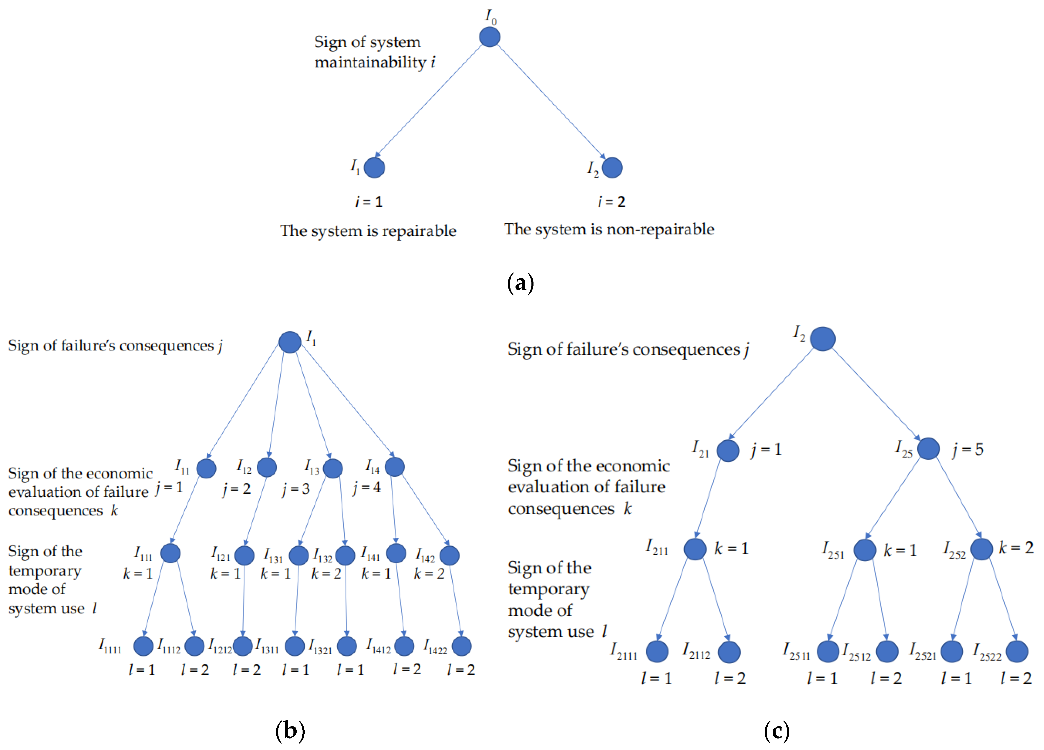
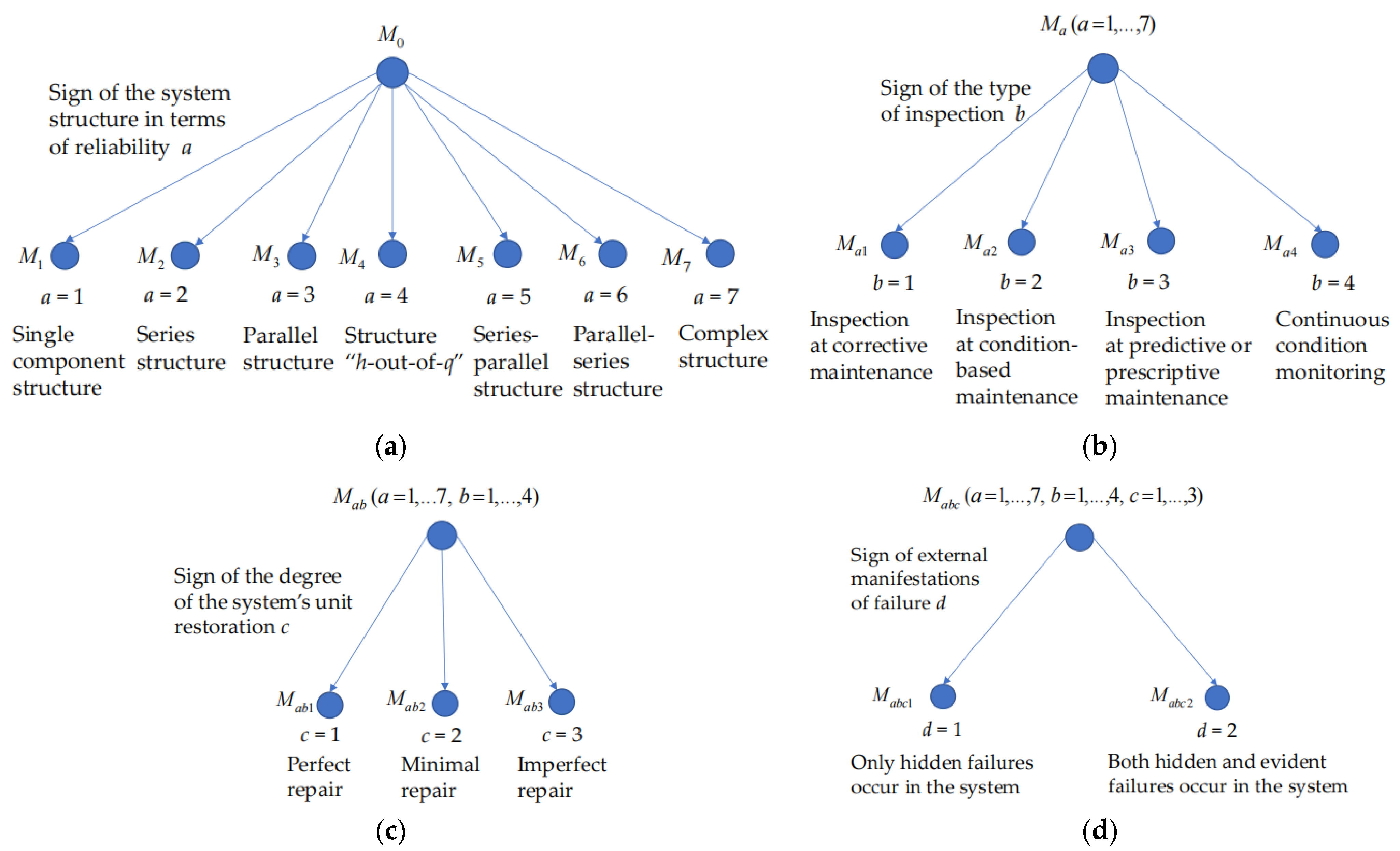
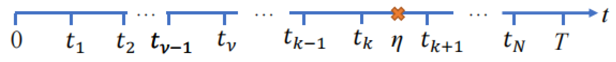
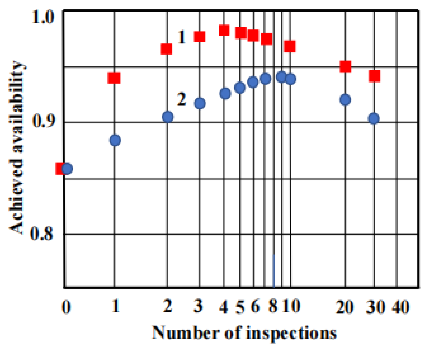
Table 1.
Subgroups of technical systems and corresponding maintenance effectiveness indicators.
| System Subgroup | Number of a Subgroup | Maintenance Effectiveness Indicators |
|---|---|---|
| I1111 | 1 | , |
| I1112 | 2 | , |
| I1212 | 3 | |
| I1311 | 4 | |
| I1321 | 5 | or |
| I1412 | 6 | |
| I1422 | 7 | or |
| I2111 | 8 | , |
| I2112 | 9 | , |
| I2511 | 10 | |
| I2512 | 11 | |
| I2521 | 12 | or |
| I2522 | 13 | or |
Table 2.
Contingency table showing the distribution of actual system conditions in rows and decisions in columns.
Table 2.
Contingency table showing the distribution of actual system conditions in rows and decisions in columns.
| Actual System Condition | Decision | |
|---|---|---|
| Positive | Negative | |
| Positive (Operable over interval (tn, tn+1)) | True positive | False negative |
| Negative 1 (Operable at time tn but inoperable over interval (tn, tn+1)) | False positive 1 | True negative 1 |
| Negative 2 (Inoperable at time tn) | False positive 2 | True negative 2 |
Disclaimer/Publisher’s Note: The statements, opinions and data contained in all publications are solely those of the individual author(s) and contributor(s) and not of MDPI and/or the editor(s). MDPI and/or the editor(s) disclaim responsibility for any injury to people or property resulting from any ideas, methods, instructions or products referred to in the content. |
© 2023 by the authors. Licensee MDPI, Basel, Switzerland. This article is an open access article distributed under the terms and conditions of the Creative Commons Attribution (CC BY) license (https://creativecommons.org/licenses/by/4.0/).
Share and Cite
MDPI and ACS Style
Ulansky, V.; Raza, A. Classification of Systems and Maintenance Models. Aerospace 2023, 10, 456. https://doi.org/10.3390/aerospace10050456
AMA Style
Ulansky V, Raza A. Classification of Systems and Maintenance Models. Aerospace. 2023; 10(5):456. https://doi.org/10.3390/aerospace10050456
Chicago/Turabian StyleUlansky, Vladimir, and Ahmed Raza. 2023. "Classification of Systems and Maintenance Models" Aerospace 10, no. 5: 456. https://doi.org/10.3390/aerospace10050456
Note that from the first issue of 2016, this journal uses article numbers instead of page numbers. See further details here.