Inverse Reinforcement Learning-Based Fire-Control Command Calculation of an Unmanned Autonomous Helicopter Using Swarm Intelligence Demonstration

Abstract

This paper concerns the fire-control command calculation (FCCC) of an unmanned autonomous helicopter (UAH). It determines the final effect of the UAH attack. Although many different FCCC methods have been proposed for finding optimal or near-optimal fire-control execution processes, most are either slow in calculational speed or low in attack precision. This paper proposes a novel inverse reinforcement learning (IRL) FCCC method to calculate the fire-control commands in real time without losing precision by considering wind disturbance. First, the adaptive step velocity-verlet iterative algorithm-based ballistic determination method is proposed for calculation of the impact point of the unguided projectile under wind disturbance. In addition, a swarm intelligence demonstration (SID) model is proposed to demonstrate teaching; this model is based on an improved particle swarm optimization (IPSO) algorithm. Benefiting from the global optimization capability of the IPSO algorithm, the SID model often leads to an exact solution. Furthermore, a reward function neural network (RFNN) is trained according to the SID model, and a reinforcement learning (RL) model using RFNN is used to generate the fire-control commands in real time. Finally, the simulation results verify the feasibility and effectiveness of the proposed FCCC method.

1. Introduction

With the development of unmanned autonomous helicopter (UAH) technology, UAHs have increasing advantages in future air warfare [1]. UAHs are cheap, with an excellent bomb load and carrying capacity, making them well suited for air-to-surface attack missions [2,3]. Moreover, UAHs are flexible, with a small turning radius and vertical takeoff capability, being able to fly close to mountains to avoid detection by enemy radar. Thus, they can perform long-range surprise attacks and post-reconnaissance strikes [4,5]. However, UAHs have poor stability because of their complex aerodynamic characteristics, making it difficult for them to achieve rapid precision attacks, especially under wind disturbance. As a result, there are growing interests in the technology of fast and precise attack using UAH automatic aiming [6], which mainly depends on the method of fire-control command calculation (FCCC).

FCCC is used to guide the weapon system to adjust the elevation angle and the azimuth angle to aim at the target to achieve the goal of a precision attack. Due to the highly coupled attitude control of the UAH, the FCCC of the UAH is a non-convex optimization problem. So far, two types of FCCC have been proposed, namely the look-up table method and the differential method. The look-up table method obtains fire-control command by multi-dimensionally, interpolating the table of the shot data or approaching this table with a continuous analytic function [7]. It has the advantage of fast calculation and meets real-time requirements. However, its shortcomings include fitting formula errors and poor universality. In addition, it needs to correct the nonlinear error of non-standard ballistic meteorological conditions using the differential method. The differential method is used to solve the ballistic differential equation [8,9] directly. It has the advantages of good universality and high precision; nevertheless, it needs multiple trajectory iterations to meet accuracy requirements, so it does not meet real-time requirements. In addition, this approach also has the danger of falling into a local optimal solution.

The traditional FCCC methods often make it challenging to balance the calculational speed and precision of the fire-control command, choosing only one to satisfy. Some improved FCCC methods have been proposed to improve the attack precision or calculational efficiency. The model in [10] can be quickly solved since there is no need to predict the status of the UAH, but it still has a significant error since the bomb is not dropped at the time of the minimum error. The method in [11] requires a long time to calculate the optimal solution, so it is difficult to apply in the rapidly changing battlefield despite high precision. Although these improved FCCC methods have further improved the speed and precision of the FCCC compared to the traditional FCCC methods, two critical issues still need to be solved.

(1)

Calculation with simultaneous consideration of the effects of disturbances and physical constraints.

(2)

Improving the precision of the attack to a sufficient level of destruction while satisfying real-time calculations.

In this paper, a new method combining the inverse reinforcement learning (IRL) algorithm with the improved particle swarm optimization (IPSO) algorithm is used to calculate the fire-control command of a UAH in real time. The main contributions of the paper are summarized as follows:

• A trajectory calculation model is established based on the system of ballistic differential equations considering the wind disturbance. The one-way adaptive step velocity-verlet algorithm is used to solve the equations iteratively. The impact point and the flight time of the unguided projectiles under wind disturbance can be computed through this model.
• A swarm intelligence demonstration (SID) model based on the IPSO algorithm is established for exact fire-control commands. This model is required to generate expert demonstrations for the latter-mentioned IRL algorithm.
• An FCCC method with the SID-based IRL (SID-IRL) structure is implemented. The RL model established in this method can learn to approximate the precision of the SID model by completing the calculation faster.

This paper is organized as follows. Section 2 introduces the related works. Section 3 details the process of the attack by a UAH with the unguided weapon. Section 4 investigates the ballistic solution with the velocity-verlet algorithm. Section 5 proposes an FCCC model using SID-IRL. Experimental simulations and comparisons between the traditional PSO algorithm, the gradient descent-based (GD) algorithm, the IPSO algorithm and the SID-IRL algorithm in two scenes are carried out in Section 6. Finally, some conclusions are presented in Section 7.

2. Related Work

Over the past few years, many improvements to the FCCC have been proposed. In [10], a control method was designed for bombing, with miss distance (MD) being calculated according to the target velocity measured by radar. Furthermore, the bombing command was executed when the MD, calculated continuously, is first found to increase. An FCCC method was proposed based on shot data in [12]. The initial solution was obtained by looking up the shot data table. Then, the fire-control commands were solved by modifying the initial solution. In [11], the relationship between th target height angle and target motion time was introduced in the solution process; in this way, the target is always considered to be a moving state in the fire-control solution process. A system of objective information acquisition, attack target selection, weapon preparation, attack preparation and formal attack was proposed based on the air-to-surface multi-target attack in [13]. The fourth-order Runge–Kutta method is applied in the fire-control computation in [14] to improve the speed of solving differential equations.

A detailed analysis of the existing proposals in the FCCC is shown in

Table 1. Relative comparison of existing proposals in FCCC.

Reference	1	2	3	4	5
Hu, X. et al. [7]	Real-time	Medium	×	×	Ability to adjust balance of precision and speed
Li, D. et al. [8]	Simulation	High	√	×	With high precision
Li, Z. et al. [11]	Simulation	High	√	√	Full consideration of the target movement
Li, X. et al. [12]	Real-time	Low	×	×	Simple structure, quick calculation
Sun, Y. et al. [13]	Simulation	-	√	×	Propose innovations for cluster attacks

1: Real-time/simulation; 2: Attack precision; 3: Universality; 4: Constraint consideration; 5: advantage; -: not-mentioned; √: considered; ×: not considered.

.

With the development of computing power, many artificial intelligence algorithms have also been used for solving nonlinear optimization problems, such as evolutionary algorithms, swarm intelligence algorithms, and machine-learning algorithms. The swarm intelligence algorithm is a computational technique based on the behavior of biological populations [15]. These algorithms solve complex combinatorial optimization problems because multiple iterative computations most likely obtain the optimal solution. However, these algorithms often need abundant computing resources and still fall into a local optimal solution. The particle swarm optimization (PSO) algorithm is one of them, with a simple structure and easy implementation. Additionally, it has a strong capability of the global search for nonlinear, multi-peaked problems [16]. Broadly, research has been done on applying PSO algorithms to unmanned aerial vehicles (UAV). In [17], a simulated annealing-particle swarm optimization algorithm was proposed to avoid local optima in UAV multi-target path planning. In [18], a PSO algorithm developed for a rapid and flexible UAV can optimize the coverage performance of the UAV. The feasibility of calculating the position command by the swarm intelligence algorithm means that the same is also possible for the attitude command. With the global optimization ability of the PSO algorithm, the angle command of the fire-control system can be calculated accurately.

However, it is difficult for the PSO algorithm to achieve a fast solution, this being precisely the advantage of machine learning. An agent trained well by the machine-learning method can be calculated by consuming few computational resources, which is suitable for deploying the machine-learning agent to on-board fire-control computers. In machine learning, the innovative deep-reinforcement learning (DRL) algorithm proposed by the DeepMind team combines methods from deep learning (DL) with powerful perception and reinforcement learning (RL) with excellent decision-making power [19]. The use of DL in RL defines the field of DRL, intending to solve the computer control problem from perception to decision-making, thus enabling general artificial intelligence. In [20], many DRL algorithms employed in automated driving were summarized. The algorithms used in automated driving give many innovative ideas for UAHs [21]. The IRL algorithm used in this paper demonstrates its strengths in performing well without explicit reward-shaping. IRL is an RL structure that aims to infer an underlying reward structure based on the interaction between the environment and expert demonstrations. It allows an agent to learn the underlying reward of the expert demonstration behavior rather than imitating surface behaviors [22]. A deep neural network was applied to the reward function structure to fit the nonlinear functions from [23,24]. In [25], an IRL algorithm was investigated to learn the UAV control performance of an expert. An inverse reinforcement learning algorithm with maximum entropy was used to increase the efficiency of the aerial combat action in [26]. In [27], an IRL using a deep Q-learning algorithm was proposed to coordinate the UAVs and the unmanned ground vehicles. The IRL algorithms are usually able to compute the output command quickly. Since the precision of the command is always close to the expert, it is essential to design a great expert demonstration model.

3. Problem Formulation

The focused problem is that air early warning (AEW) detects the target and sends the corresponding location information to the UAH. Then, the UAH, with unguided projectiles, receives information about the target, evades enemy reconnaissance, and quickly approaches the target. When the UAH’s own sensors detect the target, the UAH needs to quickly calculate the fire-control command and execute the attack mission. The process of attack by the UAH is shown in Figure 1.

Therefore, the key to calculating the fire-control problem of UAH is how to quickly generate the sequence of commands that can be executed steadily using the flight control system. In the traditional FCCC method, the FCCC model is first established, and its corresponding state vector diagram is shown in Figure 2 [28].

In this figure, ${\overrightarrow{\xi }}_{jd}$ is the displacement vector of the projectile under the effect of the initial velocity, ${\overrightarrow{\xi }}_w$ is the displacement vector under the effect of wind disturbance, $\overrightarrow{\eta }$ is the displacement vector under the effect of gravity, the relative position relationship between the UAH B and the target T is expressed by ${\overrightarrow{D}}_m$, $\overrightarrow{L}$ is the vector of predicted target displacement between current target T and the expected target $T_e$, W is the impact point of the projectile, and $\overrightarrow{e}$ is the vector of MD.

The system of the fire-control solution equations are as follows [29].

$$\begin{array}{c}\hfill t_f+D_{m}cos{\theta }_{w}cos{\psi }_w\\ \hfill =\xi \frac{u_p}{v_{01}}cos{\theta }_w^{c}cos{\psi }_w^c+\xi \frac{v_b}{v_{01}}cos\alpha cos\beta -\eta sin{\theta }_b\end{array}$$

(1)

$$\begin{array}{c}\hfill t_f+\eta cos{\theta }_{b}cos{\varphi }_b+D_{m}sin{\theta }_w=\xi \frac{u_p}{v_{01}}sin{\theta }_w^c+\xi \frac{v_b}{v_{01}}sin\alpha cos\beta \end{array}$$

(2)

$$\begin{array}{c}\hfill t_f+\eta cos{\theta }_{b}sin{\varphi }_b+D_{m}cos{\theta }_{w}sin{\psi }_w=\xi \frac{u_p}{v_{01}}cos{\theta }_w^{c}sin{\psi }_w^c\end{array}$$

(3)

where $({\xi }_{wx},{\xi }_{wy},{\xi }_{wz})$ are the wind speed constant components, $({\psi }_b,{\theta }_b,{\varphi }_b)$ are the yaw, pitch and roll of the UAH, respectively, $t_f$ is the flight time of the projectile, $D_m$ is the relative distance with $D_m=\left|{\overrightarrow{D}}_m\right|$, $\xi$ is the absolute ray length of the projectile with $\xi =|{\overrightarrow{\xi }}_{jd}|$, $u_p$ is the initial velocity of the projectile, $v_{01}$ is the absolute velocity of the projectile, $v_b$ is the velocity of the UAH, $(\alpha ,\beta )$ are the angle of attack and the angle of sideslip, $\eta =|\overrightarrow{\eta }|$, $({\theta }_w,{\psi }_w)$ are the current elevation angle and the current azimuth angle of the weapon line, while $({\theta }_w^c,{\psi }_w^c)$ are the weapon line’s expected elevation angle and azimuth angle.

The FCCC problem is to obtain the optimal values of $({\theta }_w^c,{\psi }_w^c,t_f)$ using Equations (1)–(3). However, it is difficult to solve the system of equations in real time due to the physical constraints of the UAH and the constant change in attitude angles. In addition, there are cases where the equations have no solutions after accumulating disturbance errors. Therefore, the best approach to the FCCC problem is to consider it an optimization problem. Due to the non-convex nature of the equations, the gradient-based algorithm is difficult to solve this problem because of falling into a local optimum solution.

This paper aims to integrate available target information with UAH states to compute the optimal commands of the fire-control process in real time considering the constraints. The command obtained should be reasonable for the flight control system, as it is also iteratively revised and updated until the aiming is complete. The framework of the proposed algorithm in this paper is shown in Figure 3.

4. Calculation of the Projectile’s Trajectory

The impact point of the unguided projectile, based on the current weapon angle, is first calculated by iterating through the differential equations. Then, the weapon line’s elevation angle and azimuth angle is modified so that the impact point is close to the prospective position of the target. To improve the solving speed, a neural network-fitted solution model (described in detail later) is used; thus, the precision requirement is only considered in the ballistic solving process. A variable step size velocity-verlet algorithm [30] is designed to solve the ballistic differential equations. It is assumed that the projectile has no recoil, with the initial launch velocity being constant. Since it is disturbed by the wind, wind speed should be estimated by the atmospheric wind field model.

According to the theory of external ballistics, the equations of projectiles are derived in a rectangular coordinate system as follows:

$$\left\{\begin{array}{c}{\dot{v}}_x=-f_K(v_x,z_w)\hfill \\ {\dot{v}}_y=-f_K(v_y,z_w)\hfill \\ {\dot{v}}_z=-f_K(v_z,z_w)\hfill \\ {\dot{x}}_w=v_x\hfill \\ {\dot{y}}_w=v_y\hfill \\ {\dot{z}}_w=v_z\hfill \end{array}\right.$$

(4)

where $f_K$ is the air drag function related to the velocity of the projectile itself, $v_x,v_y,v_z$ are the velocities of the projectile in the geographic coordinate system, while $(x_w,y_w,z_w)$ describes the position of the projectile.

If the projectile is consistently disturbed by cross-lateral wind during its flight, an estimate of the wind is required. So that Equation (4) is rewritten as

$$\left\{\begin{array}{c}{\dot{v}}_x=-f_K(v_x,z_w)-f_W\left({\sigma }_x\right)\hfill \\ {\dot{v}}_y=-f_K(v_y,z_w)-f_W\left({\sigma }_y\right)\hfill \\ {\dot{v}}_z=-f_K(v_z,z_w)\hfill \\ {\dot{x}}_w=v_x\hfill \\ {\dot{y}}_w=v_y\hfill \\ {\dot{z}}_w=v_z\hfill \end{array}\right.$$

(5)

where ${\sigma }_x,{\sigma }_y$ are the height-related components of wind speeds on the x-axis and y-axis, and $f_W$ is the estimated value of the wind type disturbance (to be discussed later).

4.1. The Estimation of the Wind Disturbance

Suppose that the wind has the speed $u_1$; its direction is ${\beta }_1$ for an altitude of $z_1$ obtained through the data link, $0.5 \mathrm{m}<z_1<100 \mathrm{m}$. The wind has the speed $u_b$, its direction is ${\beta }_b$ for an altitude of the airframe $z_b$ is measured by the UAH. The estimation of the wind disturbance is shown in Figure 4.

• $z_b<100 \mathrm{m}$
  In this case, the projectile is in the surface layer all the time, thus indicating the wind speed to be estimated u at the altitude z and the available wind speed $u_1$ at $z_1$ are related by a power law as follows [31]:

  $$u\left(z\right)=u_1{\left(\frac{z}{z_1}\right)}^k$$

  (6)

  with

  $$k=\ln \frac{u_b}{u_1}/\ln \frac{z_b}{z_1}$$

  (7)

  where $z_1\le z\le z_b$. The angle $\beta$ is related to ${\beta }_1$, and ${\beta }_b$ is described by

  $$\beta \left(z\right)=\frac{z_b-z}{z_b-z_1}{\beta }_1+\frac{z-z_1}{z_b-z_1}{\beta }_b$$

  (8)
• $100 \mathrm{m}\le z_b<1000 \mathrm{m}$
  In this case, the projectile is in the Ekman layer until its altitude is less than $100 \mathrm{m}$ [32]. If $0.5 \mathrm{m}\le z<100 \mathrm{m}$, it still can be calculated by Equation (6) with

  $$k\left(z\right)=1/ln[\sqrt{z·z_1}/z_0]-0.0403ln(u_1/6)$$

  (9)

  where $z_0=0.5 \mathrm{m}$ is the height of the viscous sublayer.
  The angle $\beta$ is obtained by [32]

  $$\beta \left(z\right)=\frac{z_g-z}{z_g-z_1}{\beta }_1+\frac{z-z_1}{z_g-z_1}{\beta }_g$$

  (10)

  with

  $${\beta }_g=arctan(e^{-z_g/\delta }\sin (z_g/\delta )/(1-e^{-z_g/\delta }\cos (z_g/\delta )))$$

  (11)

  where $z_g=100 \mathrm{m}$ is the critical altitude, and $\delta =1000/\pi$ is the Ekman altitude.
  If $100 \mathrm{m}\le z<z_b$, the speed u is calculated as

  $$u\left(z\right)=\frac{z_b-z}{z_b-100}{u}_g\sqrt{1-2e^{-z/\phantom{z\delta }\delta }cos\left(z/\phantom{z\delta }\delta \right)+e^{-z/\phantom{z\delta }\delta }}+\frac{z-100}{z_b-100}{u}_b$$

  (12)

  where $u_g$ is the wind speed at height $z_g$ calculated using Equations (6) and (9). The angle $\beta$ is yielded by

  $$\beta (z)=\frac{z_b-z}{z_b-100}arctan(e^{-z/\delta }\sin (z/\delta )/(1-e^{-z/\delta }\cos (z/\delta )))+\frac{z-100}{z_b-100}{\beta }_b$$

  (13)

Since the speed and angle of wind at any altitude have been obtained above, ${\sigma }_x,{\sigma }_y$ can be computed now as follows:

$$\left\{\begin{array}{c}{\sigma }_x\left(z\right)=u\left(z\right)\cos \left(\beta \left(z\right)\right)\hfill \\ {\sigma }_y\left(z\right)=u\left(z\right)\sin \left(\beta \left(z\right)\right)\hfill \end{array}\right.$$

(14)

The wind disturbance of the projectile is obtained by aerodynamic effect estimated as follows [33]:

$$\left\{\begin{array}{c}{f}_W\left({\sigma }_x\right)=\frac{1}{2}{C}_{x1}\rho {\sigma }_x^2{S}_m\hfill \\ f_W\left({\sigma }_y\right)=\frac{1}{2}{C}_{y1}\rho {\sigma }_y^2{S}_m\hfill \end{array}\right.$$

(15)

where $C_{x1}$ is the axial force coefficient, $C_{y1}$ is the sideway force coefficient, $\rho$ is the air density, while $S_m$ is the characteristic area of the projectile.

4.2. The Calculation of the Impact Point

The air drag function $f_K(v_x,z)$ can be described by [34]

$$f_K(v,z)=C\left(v\right)H\left(z\right)G\left(v\right)·v$$

(16)

with

$$\left\{\begin{array}{c}H\left(z\right)=(\mathrm{20,000}-z)/(\mathrm{20,000}+z)\hfill \\ G\left(v\right)=4.737\times {10}^{-4}·v\hfill \end{array}\right.$$

(17)

where v is the velocity of the projectile, z is the altitude of the projectile, $C\left(v\right)$ is the standard air drag coefficient, related to the Mach number of the projectile $v/\alpha$, $\alpha$ is the speed of sound, $H\left(z\right)$ is the air density function, $z\le \mathrm{10,000} \mathrm{m}$, and $G\left(v\right)$ is the air drag coefficient [35].

The initial velocity of the projectile is decomposed in the geographic coordinate system as follows:

$$\left\{\begin{array}{c}{v}_x^0=u_p·cos{\alpha }_w·cos{\beta }_w+v_{bx}\hfill \\ v_y^0=u_p·cos{\alpha }_w·sin{\beta }_w+v_{by}\hfill \\ v_z^0=u_p·sin{\alpha }_w+v_{bz}\hfill \end{array}\right.$$

(18)

where $u_p$ is the initial velocity of the projectile, $v_{bx},v_{by},v_{bz}$ are the velocities of the airframe in the geographic coordinate system, ${\alpha }_w\in \left[-\pi /2,\pi /2\right]$ is the angle between the direction of u and the horizontal plane, while ${\beta }_w\in \left[-\pi ,\pi \right]$ is the angle between the x-axis and the projection of u on the horizontal plane.

Angles ${\alpha }_w$ and ${\beta }_w$ can be calculated by the relative position between the weapon firing point and the airframe, as below:

$$\left\{\begin{array}{c}{\alpha }_w=arctan\frac{z_b-z_e}{\sqrt{{(x_b-x_e)}^2+{(y_b-y_e)}^2}}\hfill \\ {\beta }_w=arctan\frac{x_b-x_e}{y_b-y_e}\hfill \end{array}\right.$$

(19)

where $x_b,y_b,z_b$ are the coordinates of the airframe mass center, while $x_e$,$y_e$,$z_e$ are the coordinates of the weapon firing point in the geographic coordinate system; these coordinates can be calculated by [36]

$$\left[\begin{array}{c}{x}_e\\ y_e\\ z_e\end{array}\right]=T_{b\to e}·P_b$$

(20)

with

$$\begin{array}{cc}\hfill T_{b\to e}=& \left[\begin{array}{ccc}cos{\theta }_{b}cos{\psi }_b& sin{\varphi }_{b}sin{\theta }_{b}cos{\psi }_b-cos{\varphi }_{b}sin{\theta }_b& cos{\varphi }_{b}sin{\theta }_{b}cos{\psi }_b+sin{\varphi }_{b}sin{\psi }_b\\ cos{\theta }_{b}sin{\psi }_b& sin{\varphi }_{b}sin{\theta }_{b}sin{\psi }_b+cos{\varphi }_{b}cos{\psi }_b& cos{\varphi }_{b}sin{\theta }_{b}sin{\psi }_b-sin{\varphi }_{b}cos{\psi }_b\\ -sin{\theta }_b& sin{\varphi }_{b}cos{\theta }_b& cos{\varphi }_{b}cos{\theta }_b\end{array}\right]\hfill \end{array}$$

(21)

and

$$P_b=\left[\begin{array}{c}{l}_w·cos{\theta }_w·cos{\psi }_w+x_b\\ l_w·cos{\theta }_w·sin{\psi }_w+y_b\\ l_w·sin{\theta }_w+z_b\end{array}\right]$$

(22)

where $T_{b\to e}$ is the transition matrix from the airframe to the geographical coordinate system, while ${\psi }_b$, ${\theta }_b$, ${\varphi }_b$ are the airframe’s yaw, pitch and roll, respectively. $P_b$ is the initial coordinate matrix of the projectile in the airframe coordinate system, $l_w$ is the length of barrel, ${\theta }_w$ is the elevation angle of the projectile, and ${\psi }_w$ is the azimuth angle of the projectile.

The speed $v_x,v_y,v_z$ and the position $x_w,y_w,z_w$ are updated by [37]

$$\left\{\begin{array}{c}{x}_w^{j+1}=x_w^j+v_x^j\Delta t_p+\frac{{\dot{v}}_x^j}{2}\Delta t_p^2+\frac{1}{2}{f}_W({\sigma }_x(z_w^j))\Delta t_p^2\hfill \\ y_w^{j+1}=y_w^j+v_y^j\Delta t_p+\frac{{\dot{v}}_y^j}{2}\Delta t_p^2+\frac{1}{2}{f}_W({\sigma }_y(z_w^j))\Delta t_p^2\hfill \\ z_w^{j+1}=z_w^j+v_z^j\Delta t_p+\frac{{\dot{v}}_z^j}{2}\Delta t_p^2\hfill \\ v_x^{j+1}=v_x^j+\frac{{\dot{v}}_x^{j+1}-{\dot{v}}_x^j}{2}\Delta t_p+f_W({\sigma }_x(z_w^j))\Delta t_p\hfill \\ v_y^{j+1}=v_y^j+\frac{{\dot{v}}_y^{j+1}-{\dot{v}}_y^j}{2}\Delta t_p+f_W({\sigma }_y(z_w^j))\Delta t_p\hfill \\ v_z^{j+1}=v_z^j+\frac{{\dot{v}}_z^{j+1}-{\dot{v}}_z^j}{2}\Delta t_p\hfill \end{array}\right.$$

(23)

where $\Delta t_p$ is the variable step size. The impact point estimation algorithm is shown in Algorithm 1.

Algorithm 1: The one-way adaptive step velocity-verlet iterative algorithm of ballistic solution

Input: ${\varphi }_b$, ${\theta }_b$, ${\psi }_b$, $x_b$, $y_b$, $z_b$, $v_{bx}$, $v_{by}$, $v_{bz}$, $u_p$, ${\theta }_w$, ${\psi }_w$, $u_1,{\beta }_1,z_1$,$u_b,{\beta }_b,z_b$ Output: $t_f$, $x_w$, $y_w$, $z_w$ Calculate $x_e,y_e,z_e$ according to Equation (20) Calculate the initial velocities of the projectile $v_x^0,v_y^0,v_z^0$ according to Equations (18) and (19) Start iterating Initialize the initial position of the projectile with $x_w^0\leftarrow x_e,y_w^0\leftarrow y_e,z_w^0\leftarrow z_e,t_f\leftarrow 0$ Initialize iteration index $j=1$, iteration step $\Delta t_p=0.5$, attenuation factor $k=1$ while $z_w^j>0.01$ do    Calculate the wind disturbance $f_W\left({\sigma }_x\left(z_w\right)\right),f_W\left({\sigma }_y\left(z_w\right)\right)$ at $z_w^j$ by Equation (15)    Calculate $v_x^{j+1},v_y^{j+1},v_z^{j+1},x_w^{j+1},y_w^{j+1},z_w^{j+1}$ by Equation (23)    if $z_w^{j+1}$ < 0 then        Update $\Delta t_p={(\frac{z_w^j}{z_w^j-z_w^{j+1}})}^k\Delta t_p$        Recalculate $v_x^{j+1},v_y^{j+1},v_z^{j+1},x_w^{j+1},y_w^{j+1},z_w^{j+1}$ with new $\Delta t_p$        Increase $k=k+1$    end if    Update $j=j+1$    Record $t_f=t_f+\Delta t_p$ end while Record $x_w=x_w^j,y_w=y_w^j,z_w=z_w^j$

5. Fire-Control Command Calculation Method Based on SID-IRL

After establishing the trajectory calculation approach, the FCCC method can be designed by the virtual MD between the impact point calculated in Section 3 and the expected position of the target. This method is based on the following idea:

First, expert demonstrations are obtained by the SID model; then, the IPSO algorithm is used to iteratively optimize the elevation and the azimuth angles of the projectile in the SID model. Afterwards, the expert demonstrations are used to train a reward function. Finally, the IRL algorithm is used to learn the reward function, then a fast iterative and precision FCCC model is obtained.

5.1. The Establishment of the Swarm Intelligence Demonstration Model

In this model, the elevation and the azimuth angles of the projectile are used as variables to optimize. Then, the final command curve of the optimal angles in solution space is obtained using the MD and aiming time as evaluation indicators.

The projectile flight time and the expected MD are obtained by the trajectory calculation model with the current projectile’s elevation and azimuth angles. The firing condition is judged to be complete; if not, the fitness function is optimized according to the IPSO algorithm. The fitness function of the IPSO algorithm can be calculated by

$$F_{fit}=w_1·\left|\overrightarrow{e}\right|+w_2·t_f$$

(24)

where $w_1$ is the weighting factor of MD, $w_2$ is the weighting factor of the flight time of the projectile, and $t_f$ is the flight time of the projectile. $\left|\overrightarrow{e}\right|$ is the virtual MD calculated by the projectile’s impact point and the target’s expected position; the former is obtained by Algorithm 1, while the latter is calculated as follows:

$$\left|\overrightarrow{e}\right|=\sqrt{{(x_{te}-x_w)}^2+{(y_{te}-y_w)}^2+{(z_{te}-z_w)}^2}$$

(25)

with

$$\left\{\begin{array}{c}{x}_{te}=x_t+v_{tx}·t_f\hfill \\ y_{te}=y_t+v_{ty}·t_f\hfill \\ z_{te}=z_t+v_{tz}·t_f\hfill \end{array}\right.$$

(26)

where $x_{te},y_{te},z_{te}$ express the expected position of the target at the time of the projectile landing, $x_t,y_t,z_t$ denotes the position of the target at the time of the projectile firing, and $v_{tx},v_{ty},v_{tz}$ are the velocities of the target.

Due to the execution time required to apply the command to the flight control system, calculating the final result fails to meet the fast-aiming requirement. It neglects the effect of the airframe’s inertia during the iterative process. As a result, the traditional PSO must be improved by spatial clipping so that the command of each iteration can be applied as the current control expectation. In each iteration, the maximum and minimum constraints of the projectile’s elevation and azimuth angles are simultaneously updated, considering the inertia of the airframe’s rotation. The update of the constraints is shown in Equation (27).

$$\left\{\begin{array}{c}{\theta }_{max}^{i+1}={\theta }_w^i+{\lambda }_d{w}_{\theta }^i\Delta t_j+\frac{1}{2}{\beta }_{\theta }\Delta {t_j}^2\hfill \\ {\psi }_{max}^{i+1}={\psi }_w^i+{\lambda }_d{w}_{\psi }^i\Delta t_j+\frac{1}{2}{\beta }_{\psi }\Delta {t_j}^2\hfill \\ {\theta }_{min}^{i+1}={\theta }_w^i+{\lambda }_d{w}_{\theta }^i\Delta t_j-\frac{1}{2}{\beta }_{\theta }\Delta {t_j}^2\hfill \\ {\psi }_{min}^{i+1}={\psi }_w^i+{\lambda }_d{w}_{\psi }^i\Delta t_j-\frac{1}{2}{\beta }_{\psi }\Delta {t_j}^2\hfill \end{array}\right.$$

(27)

where ${\theta }_w^i$, ${\psi }_w^i$ are the elevation and the azimuth angle of the projectile at i, $\left[{\theta }_{min}^i,{\theta }_{max}^i\right]$, and $\left[{\psi }_{min}^i,{\psi }_{max}^i\right]$ are the bounded ranges, and $w_{\theta }^i$, $w_{\psi }^i$ are the velocities, ${\beta }_{\theta }$, ${\beta }_{\psi }$ are the maximum angular acceleration of them, ${\lambda }_d\in (0,1)$ is the damping term, while $\Delta t_j$ is the iteration step of FCCC.

The improvement of the PSO algorithm is based on spatial clipping by updating the constraints at every iteration. It helps reduce the situation of being in a local optimum solution and improves the computation speed and precision. The following diagram of the IPSO algorithm is shown in Figure 5. We make the max iteration of the SID model be $I_{max}$, the fitness allowed for attack $F_{attack}$, and the expert demonstrations generated by the SID model are shown in Algorithm 2.

Algorithm 2: Expert demonstrations generation algorithm

Input: Parameters of the environment, ${\theta }_w^0,{\psi }_w^0$ Output: $\{{\theta }_w^1,{\theta }_w^2,\cdots \}$, $\{{\psi }_w^1,{\psi }_w^2,\cdots \}$ Calculate $x_w,y_w,z_w,t_f$ with ${\theta }_w^0,{\psi }_w^0$ according to Algorithm 1 Calculate $F_{fit}$ by Equation (24) Initialize $i=1$ while $i<I_{\max }$ or $F_{fit}>F_{attack}$ do    Update $i=i+1$    Spatial clipping according to Equation (27)    Find the best ${\theta }_w^i,{\psi }_w^i$ by IPSO algorithm    Calculate $x_w,y_w,z_w,t_f$ with ${\theta }_w^i,{\psi }_w^i$    Calculate $F_{fit}$ by Equation (24) end while

5.2. The Establishment of SID-IRL Model

The swarm intelligence algorithm requires a large population size to meet the solution precision, which often leads to a long solution time and cannot meet the requirement of fast aiming. The IRL algorithm is considered in order to use the environment state and its state to obtain the reward function effectively. Then, it learns the optimal solution command through the generated reward function, which can improve the solution efficiency without affecting the precision of the solution.

The parameters that affect the solution results are used as the input of the IRL algorithm; they are shown in

Table 2. The parameters of input.

Name	Meaning
$v_{bx}$, $v_{by}$, $v_{bz}$	Velocity of the airframe in the geographic coordinate system
$v_{tx}$, $v_{ty}$, $v_{tz}$	Velocity of the target in the geographic coordinate system
$u_p$	initial velocity of the projectile
$a_{tx}$, $a_{ty}$, $a_{tz}$	acceleration of the target in the geographic coordinate system
$x_b$, $y_b$, $z_b$	Position of the airframe in the geographic coordinate system
$x_t$, $y_t$, $z_t$	Position of the target in the geographic coordinate system
${\theta }_{max}$, ${\theta }_{min}$	The maximum and the minimum of the projectile elevation angle
${\psi }_{max}$, ${\psi }_{min}$	The maximum and the minimum of the projectile azimuth angle

.

The output $\chi$ of the SID model and the output $\gamma$ of the IRL agent is used to train the reward function of the neural network (RFNN) model. First, the IRL agent is initialized randomly, with the same set of environment parameters being used as the input of both the SID model and the IRL agent. Then, the RFNN is trained to reach the goal that outputs a higher value $R\left(\chi \right)$ with the input of $\chi$ while outputting a lower value $R\left(\gamma \right)$ with the input of $\gamma$. An RFNN model can evaluate the behavior of the SID model as better behavior is obtained. Finally, the RFNN model trains the IRL agent with the deep deterministic policy gradient (DDPG) algorithm [38]. The diagram of the SID-IRL algorithm is shown in Figure 6.

6. Simulation Results

In this section, two simulations are performed to verify the feasibility and the effectiveness of the proposed model and algorithm in the quick calculation fire-control problem:

(1)

The UAH approaches from a distance after knowing the target’s location and drops bombs.

(2)

The UAH suddenly finds the target in the process of close reconnaissance and makes timely adjustments to attack.

In the SID-IRL model, we use Adam [39] for learning the neural network parameters with a learning rate of $5\times {10}^{-4}$, $5\times {10}^{-3}$ and $5\times {10}^{-4}$ for the actor, critic network and RFNN. The actor network has two hidden layers with 400 and 300 units, respectively; the units of its input and output layers are 20 and 2, respectively. The critic network has one hidden layer with 500 units. Moreover, the RFNN has three hidden layers with 200, 500, and 100 units, respectively. The size of the SID-IRL model’s experience pool is set to 200,000. The main parameters of SID are shown in

Table 3. The main parameters of the SID.

Name	Meaning	Value
$N_{si}$	Population quantity	100
$D_{si}$	Particle dimension	2
$T_{si}$	Maximum Iterations	200
$c_1$	Learning factor 1	0.5
$c_2$	Learning factor 2	0.5
$W_{\max }$	Maximum inertia weight	0.8
$W_{\min }$	Minimum inertia weight	0.4
$V_{\max }$	Maximum velocity weight	0.5
$V_{\min }$	Minimum velocity weight	$-0.5$

.

The actor network trained by the above parameters will act as the agent as the output of the proposed algorithm. In the following experiments, the performance of the SID-IRL algorithm is evaluated by the MD, the earliest attackable time of the UAH, and the calculation time. We compared the results with the traditional PSO algorithm, the GD algorithm, and the IPSO algorithm with and without wind disturbance.

6.1. Case 1: Long-Range Attack

In this scenario, the UAH is set at a remote location away from the target and fires an unguided weapon to launch an attack. Furthermore, the UAH moves at a higher velocity, while the target does not detect the presence of the UAH and thus moves at a low speed. The speed and direction of the wind at the height of the UAH are known, and the surface wind data are known from the monitoring-station measurements. The main parameters of case 1 are shown in

Table 4. The main parameters of the simulation case 1.

Name	Value	Unit
$v_{bx},v_{by},v_{bz}$	50, 0, 0	m/s
$v_{tx},v_{ty},v_{tz}$	10, 10, 0	m/s
$u_p$	500	m/s
$x_b,y_b,z_b$	0, 0, 500	m
$x_t,y_t,z_t$	2000, 800, 0	m
$a_{tx},a_{ty},a_{tz}$	1, 1, 0	m/s${}^2$
${\psi }_b,{\theta }_b,{\varphi }_b$	0, $-5$, 0	Deg
$u_1,u_b$	1, 5	m/s
${\beta }_1,{\beta }_b$	5, 20	m/s
$z_1$	5	m

.

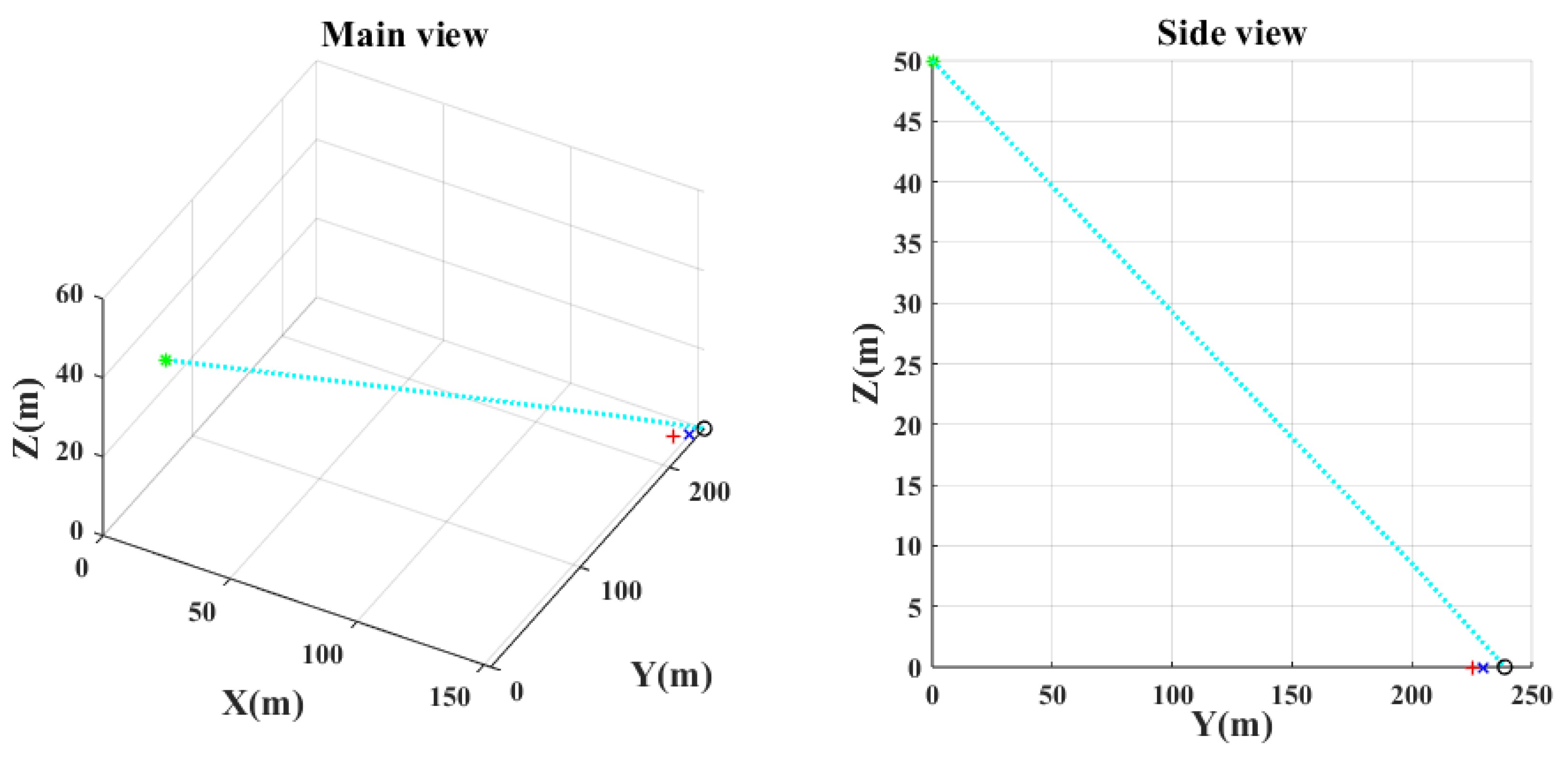
Figure 7, Figure 8, Figure 9 and Figure 10 show the main and the side views of the projectile trajectory when the final attack command is given with FCCC by different algorithms. The green asterisk represents the position of the UAH at this moment. The light blue dotted line shows the projectile’s trajectory. The black circle denotes the impact point. The red plus indicates where the target was at launch. The blue cross indicates the expected target position. 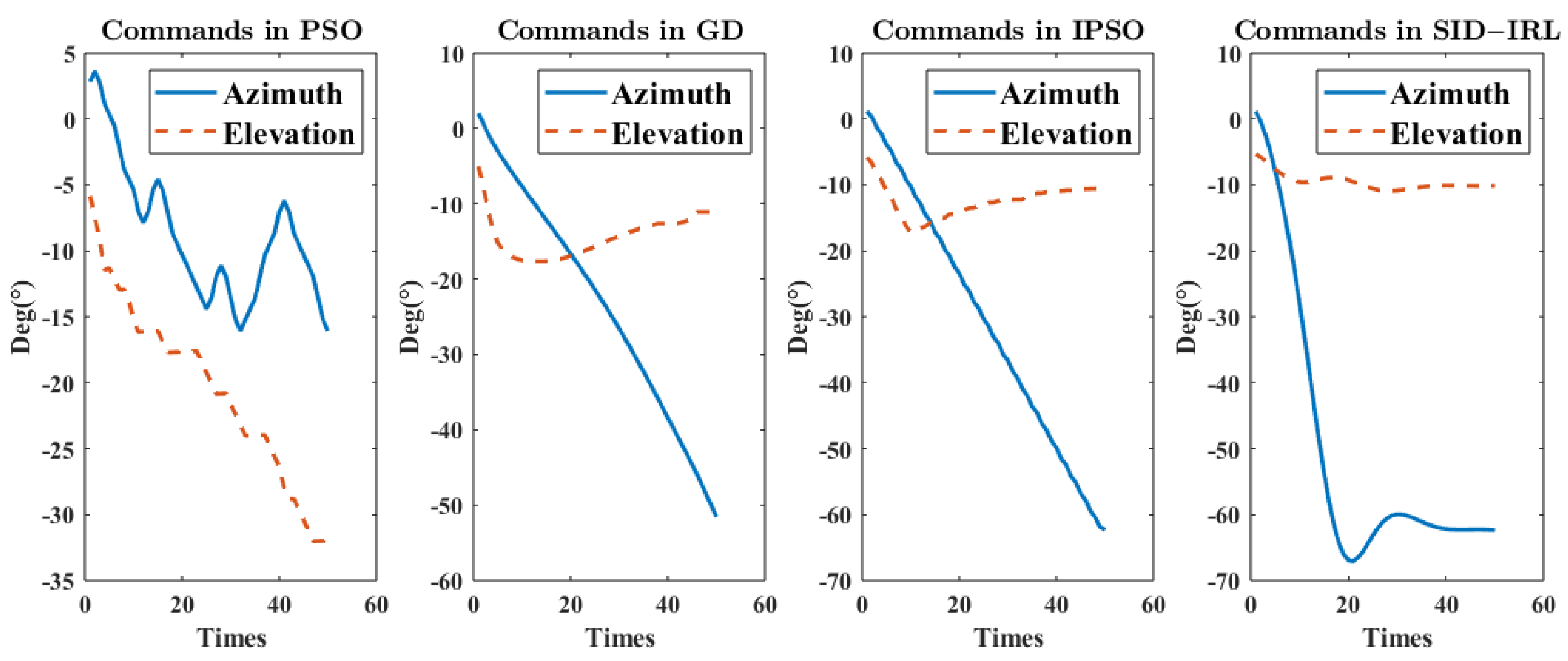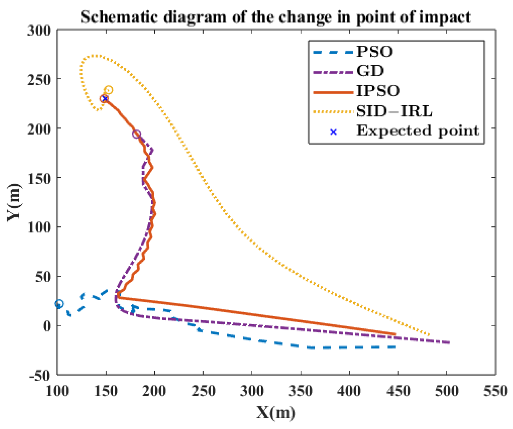Figure 11 shows the sequence of commands calculated by different algorithms. The change in the virtual impact point in different algorithms is shown in Figure 12. 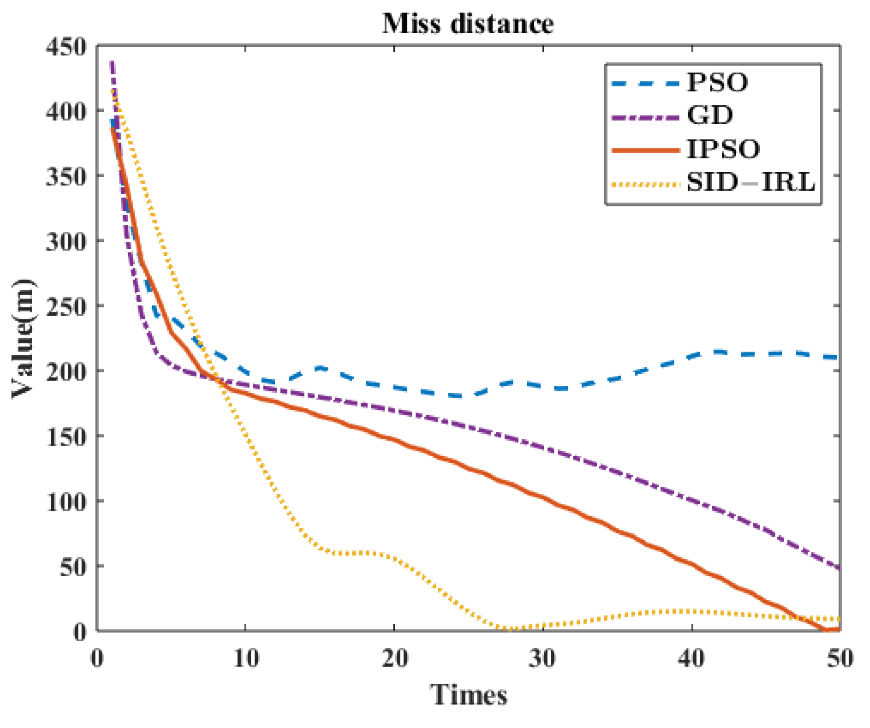Figure 13 shows the MD of the projectile over time in different algorithms. The comparison results of this case in 5 s between the PSO algorithm, GD algorithm, IPSO algorithm and SID-IRL algorithm are shown in

Table 5. Comparison results of case 1.

Wind	Method	1	2	3	4	5	6	7	8	9
×	PSO	806.17	1192.39	1024.22	129.83	inf	154.11	160.65	156.97	2.24
×	GD	21.35	26.79	24.23	1.90	4.2	9.21	9.69	9.39	0.18
×	IPSO	1.95	6.71	4.30	1.63	5.5	108.77	116.54	112.82	2.81
×	SID-IRL	54.92	56.85	55.84	0.68	inf	1.98	2.16	2.04	0.06
√	PSO	646.06	1263.68	975.21	239.79	inf	164.28	178.80	173.01	4.76
√	GD	17.72	17.73	17.73	0.01	2.4	7.42	7.87	7.62	0.18
√	IPSO	0.02	0.15	0.09	0.05	2.1	124.00	127.46	125.98	1.32
√	SID-IRL	38.75	38.89	38.83	0.05	0.7	2.04	2.23	2.09	0.07

1: Minimum of the MD(m); 2: Maximum of the MD(m); 3: Mean of the MD(m); 4: Standard deviation of the MD; 5: Earliest attackable time(s); 6: Minimum time of the calculation(s); 7: Maximum time of the calculation(s); 8: Mean time of the calculation(s); 9: Standard deviation of the calculational time.

.

6.2. Case 2: Close-Range Attack

In this scenario, the UAH is on patrol at a low altitude. Assume that when the UAH finds the target, the target makes a fast movement to avoid the attack. Because the UAH is at a lower altitude, it can be assumed that the wind speed at the altitude of the airframe is the same as the wind speed near the ground. The main parameters of case 2 are shown in

Table 6. The main parameters of the simulation case 2.

Name	Value	Unit
$v_{bx},v_{by},v_{bz}$	5, 0, 0	m/s
$v_{tx},v_{ty},v_{tz}$	25, 25, 0	m/s
u	500	m/s
$x_b,y_b,z_b$	0, 0, 50	m
$x_t,y_t,z_t$	120, 200, 0	m
$a_{tx},a_{ty},a_{tz}$	0, 0, 0	m/s${}^2$
${\psi }_b,{\theta }_b,{\varphi }_b$	2, $-5$, 0	Deg
$u_1,u_b$	1, 1	m/s
${\beta }_1,{\beta }_b$	20, 20	m/s
$z_1$	5	m

.

Figure 14, Figure 15, Figure 16 and Figure 17 show the final projectile trajectory’s main and side views in this case. The marker description is the same as in case 1. Figure 18 shows the sequence of commands calculated by different algorithms in this case. Figure 19 shows the change in the virtual impact point by different algorithms in this case. The MD of the projectile over time is shown in Figure 20. In

Table 7. Comparison results of case 2.

Wind	Method	1	2	3	4	5	6	7	8	9
×	PSO	195.64	225.43	215.80	10.46	inf	69.28	86.77	77.36	7.26
×	GD	52.54	59.60	55.80	2.35	inf	8.45	8.88	8.66	0.16
×	IPSO	1.99	4.36	2.69	0.86	4.7	50.17	59.21	55.96	3.24
×	SID-IRL	11.92	12.15	12.01	0.09	2.3	1.99	2.12	2.04	0.05
√	PSO	178.82	227.01	201.81	16.65	inf	72.43	98.87	91.26	9.56
√	GD	47.81	47.84	47.83	0.01	5.0	6.95	7.58	7.08	0.25
√	IPSO	1.48	1.55	1.51	0.02	4.1	60.40	61.16	60.61	0.29
√	SID-IRL	9.15	9.75	9.31	0.02	2.1	2.16	2.43	2.25	0.09

1: Minimum of the MD(m); 2: Maximum of the MD(m); 3: Mean of the MD(m); 4: Standard deviation of the MD; 5: Earliest attackable time(s); 6: Minimum time of the calculation(s); 7: Maximum time of the calculation(s); 8: Mean time of the calculation(s); 9: Standard deviation of the calculational time.

, the comparative data of each algorithm is presented.

From these experimental results, we have the following observations.

(1)

As shown in Figure 7 and Figure 14, the FCCC method using the traditional PSO algorithm makes it difficult to find optimal or suboptimal solutions in an extensive range. It remains in an untargeted completion state at the final moment. However, the IPSO algorithm can precisely aim at the target because of the clipping of the search space and the consideration of physical constraints, as shown in Figure 9 and Figure 16. The global search capability of the IPSO algorithm is significantly increased, allowing it to satisfy the precision requirements fully. However, according to Table 5 and Table 7, the calculation speed of the IPSO algorithm is far from the real-time requirement. Moreover, the SID-IRL algorithm proposed in this paper provides a result slightly worse than the IPSO algorithm in MD, but has far better calculational efficiency, according to Table 5 and Table 7.

(2)

The gradient-based algorithm of FCCC can obtain a solution at a fast computational speed, but it does not attack with great precision, as shown in Table 5 and Table 7. Although the gradient algorithm used has an adaptive step size, the result is still not optimal for each iteration. In addition, the method can meet real-time requirements well, but its lack of attack accuracy prevents it from being a demonstration model.

(3)

With the consideration of wind disturbance, the mean MD of SID-IRL drops from 56.85 to 38.89 in case 1, which satisfies the condition of attack (MD $<50$). The cost of the calculation for wind disturbance is an increase in computational load, which increases its computation time, but the gain in the precision of attack is as expected.

(4)

By combining Figure 11 and Figure 12, it can be seen that the SID-IRL algorithm adjusts both the x-axis orientation and y-axis orientation to bring the virtual impact point close to the expected point as quickly as possible. It makes the earliest attackable time of the SID-IRL algorithm even better than the IPSO algorithm. We think the right policy is obtained by the IRL algorithm through inverse learning. By acquiring the potential rewards, the SID-IRL model performs better than the demonstrator system of the IPSO algorithm.

(5)

As shown in Figure 11 and Figure 18, the SID-IRL algorithm generates more logical commands to stabilize the azimuth to the expected angle more quickly. The smooth commands generated by the SID-IRL algorithm are better for UAH’s flight control system to respond. Moreover, as can be seen from the azimuth angle commands sequence in Figure 11 and Figure 18, the commands of the SID-IRL algorithm quickly arrive near the desired angle and slowly converge.

(6)

The comparison results of the two simulation scenarios show that the SID-IRL algorithm has a more attractive performance in the scenario of the close-range attack. It allows the UAH to react quickly to complete targeting attacks in a sudden environment, thus enormously increasing the UAH survival rate and effectively reducing the possibility of enemy escape.

7. Conclusions

The purpose of this paper is to calculate the fire-control command of a UAH in real time, given the wind interference and flight constraints. In this paper, an IRL-based FCCC method has been proposed with the demonstration of the swarm intelligence algorithm. First, an iterative method of adaptive step velocity-verlet algorithm for ballistic trajectory calculation under wind disturbance has been proposed. In addition, a SID model for FCCC through an IPSO algorithm has been established, which can obtain fire-control commands with high precision. Subsequently, the RFNN has been trained by the IRL algorithm and the SID demonstrative teaching. Finally, the agent has been trained with the policy of DDPG and the reward function from the RFNN. The fire-control computer with the agent model can quickly output fire-control commands according to its own and environment states. In the simulation, the IRL-based FCCC method has been compared with the PSO algorithm, the GD algorithm and the IPSO algorithm in two scenarios of the long-range attack and close-range attack. The simulation results show that the IRL-based FCCC method has precision similar to the demonstrations of SID. Additionally, the calculational efficiency of the IRL-based FCCC method is superior to the PSO algorithm and the GD algorithm. On the other hand, from the perspective of time complexity, if the number of fire-control command sequences is n, the time complexity of the final agent is approximately $O\left(D_{si}n\right)$, which is less than the time complexity of the PSO algorithm ($O\left(N_{si}{D}_{si}{T}_{si}n\right)$). Overall, we can conclude that the proposed IRL-based method works well for the FCCC for UAH. This is crucial in the application of the observation strike integrated UAH. However, the proposed method’s precision is still not sufficient for destroying ground-moving targets with high maneuverability. Thus, further improvements to the attack precision of the FCCC algorithm are needed in future work.

References

- Nguyen, V.N.; Jenssen, R.; Roverso, D. Automatic Autonomous Vision-based Power Line Inspection: A review of Current Status and the Potential Role of Deep Learning. Int. J. Electr. Power Energy Syst. 2018, 99, 107–120. [Google Scholar] [CrossRef] [Green Version]
- Devasia, S.; Lee, A. A Scalable Low-Cost Unmanned-Aerial-Vehicle Traffic Network. J. Air Transp. 2016, 24, 74–83. [Google Scholar] [CrossRef] [Green Version]
- Mahony, R.; Kumar, V.; Corke, P. Multirotor Aerial Vehicles Modeling, Estimation, and Control of Quadrotor. IEEE Robot. Autom. Mag. 2012, 19, 20–32. [Google Scholar] [CrossRef]
- Oktay, T.; Celik, H.; Turkmen, I. Maximizing Autonomous Performance of Fixed-wing Unmanned Aerial Vehicle to Reduce Motion Blur in Taken Images. Proc. Inst. Mech. Eng. Part I J. Syst. Control. Eng. 2018, 232, 857–868. [Google Scholar] [CrossRef]
- Liu, C.; Ding, F.; Wang, G.; Gao, F.; Ding, F.; Bao, C.; Guo, X.; Li, C.; Yi, Z. Pint-Sized Airborne Fire Control System of UAV and its Key Technology. In Advances in Intelligent and Soft Computing, Proceedings of the 6th International Conference on Intelligent Systems and Knowledge Engineering (ISKE 2011), Shanghai, China, 15–17 December 2011; Wang, Y., Li, T., Eds.; Springer: Berlin/Heidelberg, Germany, 2011; Volume 124, pp. 477–483. [Google Scholar]
- Cao, Z.; Mao, Y.; Deng, C.; Liu, Q.; Chen, J. Research of Maneuvering Target Prediction and Tracking Technology based on IMM Algorithm. In Proceedings of SPIE, Proceedings of the 8th International Symposium on Advanced Optical Manufacturing and Testing Technologies: Optical Test, Measurement Technology, and Equipment, Suzhou, China, 26–29 April 2016; Zhang, Y., Wu, F., Xu, M., To, S., Eds.; SPIE: Bellingham, WA, USA, 2016; Volume 9684, pp. 757–763. [Google Scholar]
- Hu, X.; Ma, G.; Ge, J. Research on Method of Solving Fire Control Command for Multi-rotor UAV. J. Ordnance Equip. Eng. 2018, 39, 33–38. [Google Scholar]
- Li, D. Fourth-order Runge-Kutta Method is Applied in the Fire Control Computation. Microcomput. Inf. 2011, 27, 192–193. [Google Scholar]
- Pu, H.; Liu, M.; Wang, H.; Cai, W. UCAV NWL Bombing Accuracy Analyis Based on Communication Lag environment. Fire Control. Command. Control. 2017, 42, 110–113. [Google Scholar]
- Chen, H.; Xie, J. The Establishment of Unmanned Bomber’s Aiming Equation and its Simulation. J. Proj. Rocket. Missiles Guid. 2007, 1, 231–234. [Google Scholar]
- Li, Z.; Wu, P. Improved Algorithm and Model Simulation for Anti-aircraft Fire Control Based on External Ballistics. Command. Control. Simul. 2021, 43, 18–24. [Google Scholar]
- Li, X.; Liu, J.; Wang, Q.; Rong, M. Research of Tank Fire Control System Firing Data Resolving Simulative Model. Fire Control. Command. Control. 2008, 33, 126–138. [Google Scholar]
- Sun, Y. Design on Air-to-surface Muti-target Attack for Fire Control System. Ind. Innov. 2018, 5, 13–17. [Google Scholar]
- Gan, J. Low-Speed Target Motion Analysis and Hit Parameters Solving. Master’s Thesis, Nanjing University of Science and Technology, Nanjing, China, 2010. [Google Scholar]
- Kennedy, J. Handbook of Nature-Inspired and Innovative Computing: Integrating Classical Models with Emerging Technologies; Zomaya, A.Y., Ed.; Springer: Boston, MA, USA, 2006; pp. 187–219. ISBN 978-0-387-27705-9. [Google Scholar]
- Kennedy, J.; Eberhart, R. Particle Swarm Optimization. In Proceedings of the 1995 IEEE International Conference on Neural Networks (ICNN 95), Perth, Australia, 27 October–1 November 1995; Volume 4, pp. 1942–1948. [Google Scholar]
- Huang, Q.; Sheng, Z.; Fang, Y.; Li, J. A Simulated Annealing-Particle Swarm Optimization Algorithm for UAV Multi-target Path Planning. In Proceedings of the 2022 2nd International Conference on Consumer Electronics and Computer Engineering (ICCECE), Guangzhou, China, 14–16 January 2022; pp. 906–910. [Google Scholar]
- Zhan, Y.; Zhan, L.; Liu, C. 3-D Deployment Optimization of UAVs based on Particle Swarm Algorithm. In Proceedings of the 2019 IEEE 19th International Conference on Communication Technology (ICCT), Xi’an, China, 16–19 October 2019; pp. 954–957. [Google Scholar]
- Arulkumaran, K.; Deisenroth, N.P.; Brundage, M.; Bharath, A.A. Deep Reinforcement Learning A brief survey. IEEE Signal Process. Mag. 2017, 34, 26–38. [Google Scholar] [CrossRef] [Green Version]
- Kiran, B.R.; Sobh, I.; Talpaert, V.; Mannion, P.; Al Shallab, A.A.; Yogamani, S.; Perez, P. Deep Reinforcement Learning for Autonomous Driving: A Survey. IEEE Trans. Intell. Transp. Syst. 2021, 23, 4906–4926. [Google Scholar] [CrossRef]
- Azar, A.T.; Koubaa, A.; Ali Mohamed, N.; Ibrahim, H.A.; Ibrahim, Z.F.; Kazim, M.; Ammar, A.; Benjdira, B.; Khamis, A.M.; Hameed, I.A.; et al. Drone Deep Reinforcement Learning: A Review. Electronics 2021, 10, 999. [Google Scholar] [CrossRef]
- Wulfmeier, M.; Ondruska, P.; Posner, I. Maximum Entropy Deep Inverse Reinforcement Learning. arXiv 2015, arXiv:1507.04888. [Google Scholar]
- Bengio, Y.; Courville, A.C.; Vincent, P. Unsupervised Feature Learning and Deep Learning: A Review and new Perspectives. arXiv 2012, arXiv:1206.5538v1. [Google Scholar]
- Mnih, V.; Kavukcuoglu, K.; Silver, D.; Graves, A.; Antonoglou, L.; Wierstra, D.; Riedmiller, M. Playing Atari with Deep Reinforcement Learning. arXiv 2013, arXiv:1312.5602. [Google Scholar]
- Choi, S.; Kim, S.; Kim, H.J. Inverse Reinforcement Learning Control for Trajectory Tracking of a Multirotor UAV. Int. J. Control. Autom. Syst. 2017, 15, 1826–1834. [Google Scholar] [CrossRef]
- Kong, W.; Zhou, D.; Yang, Z.; Zhao, Y.; Zhang, K. UAV Autonomous Aerial Combat Maneuver Strategy Generation with Observation Error based on State-adversarial Deep Deterministic Policy Gradient and Inverse Reinforcement Learning. Electronics 2020, 9, 1121. [Google Scholar] [CrossRef]
- Nguyen, H.T.; Garratt, M.; Bui, L.T.; Abbass, H. Apprenticeship Bootstrapping: Inverse Reinforcement Learning in a Multi-skill UAV-UGV Coordination Task. In Proceedings of the 17th International Conference on Autonomous Agents and MultiAgent Systems (AAMAS), Stockholm, Sweden, 10–15 July 2018; pp. 2204–2206. [Google Scholar]
- Huang, Y.; He, J.; Zhou, M.; Gao, C. Researching Integrated Flight / Fire Control System of Air-to-Ground Guided Bombs. J. Northwestern Polytech. Univ. 2016, 34, 275–280. [Google Scholar]
- Li, Y. Anti-Disturbance Flight Control for Unmanned Helicopter under Stochastic Disturbances. Master’s Thesis, Nanjing University of Aeronautics and Astronautics, Nanjing, China, 2020. [Google Scholar]
- Papadopoulos, D.F.; Simos, T.E. The Use of Phase Lag and Amplification Error Derivatives for the Construction of a Modified Runge-Kutta-Nystrom Method. Abstract and Applied Analysis. Abstr. Appl. Anal. 2013, 2013, 910624. [Google Scholar] [CrossRef]
- Wang, W. Atmospheric Wind Field Modeling and its Application. Master’s Thesis, National University of Defense Technology, Changsha, China, 2009. [Google Scholar]
- Lieberman, R. The Gradient Wind in the Mesosphere and Lower Thermosphere. Earth Planets Space 1999, 51, 751–761. [Google Scholar] [CrossRef] [Green Version]
- Tian, X.; Meng, C.; Ma, J.; Ma, B.; Wang, Y.; Chen, W. Research on Structure and Fire Control System of Fire Fighting UAV Based on Polymer Gel Fire Bomb. In Proceedings of the 2022 IEEE 10th Joint International Information Technology and Artificial Intelligence Conference (ITAIC), Chongqing, China, 17–19 June 2022; Volume 10, pp. 842–845. [Google Scholar]
- Wessam, M.E.; Chen, Z. Aerodynamic Characteristics of Unguided Artillery Projectile. Adv. Mater. Res. 2014, 1014, 165–168. [Google Scholar] [CrossRef]
- Han, Z.; Chen, M.; Shao, S.; Wu, Q. Improved Artificial Bee Colony Algorithm-based Path Planning of Unmanned Autonomous Helicopter Using Multi-strategy Evolutionary Learning. Aerosp. Sci. Technol. 2022, 122, 107374. [Google Scholar] [CrossRef]
- Yan, K. Robust Fault Tolerant Constrained Control for Unmanned Autonomous Helicopter. Master’s Thesis, Nanjing University of Aeronautics and Astronautics, Nanjing, China, 2020. [Google Scholar]
- Elbes, M.; Alzubi, S.; Kanan, T.; Hawashin, B. A Survey on Particle Swarm Optimization with Emphasis on Engineering and Network Applications. Evol. Intell. 2019, 12, 113–129. [Google Scholar] [CrossRef]
- Hou, Y.; Liu, L.; Wei, Q.; Xu, X.; Chen, C. A Novel DDPG Method with Prioritized Experience Replay. In Proceedings of the 2017 IEEE International Conference on Systems, Man, and Cybernetics (SMC), Banff, AB, Canada, 5–8 October 2017; pp. 316–321. [Google Scholar]
- Kingma, D.; Ba, J. Adam: A method for stochastic optimization. arXiv 2014, arXiv:1412.6980. [Google Scholar]
Figure 1.
The attack process of UAH.
Figure 2.
The schematic diagram of the fire-control command calculation method.
Figure 3.
The framework of SID-IRL fire-control command calculation method.
Figure 4.
The schematic diagram of the wind disturbance estimation.
Figure 5.
The follow diagram of the IPSO algorithm.
Figure 6.
The flow diagram of the SID-IRL model.
Figure 7.
The ballistic of PSO in case 1.
Figure 8.
The ballistic of GD in case 1.
Figure 9.
The ballistic of IPSO in case 1.
Figure 10.
The ballistic of SID-IRL in case 1.
Figure 11.
Command of the projectile angles in case 1.
Figure 12.
Change of impact point in case 1.
Figure 13.
Miss distance in case 1.
Figure 14.
The ballistic of PSO in case 2.
Figure 15.
The ballistic of GD in case 2.
Figure 16.
The ballistic of IPSO in case 2.
Figure 17.
The ballistic of SID-IRL in case 2.
Figure 18.
Command of the projectile angles in case 2.
Figure 19.
Change of impact point in case 2.
Figure 20.
Miss distance in case 2.