Article

Aerodynamic Thermal Simulation and Heat Flux Distribution Study of Mechanical Expansion Reentry Vehicle

School of Astronautics, Beihang University, Beijing 100191, China
*
Author to whom correspondence should be addressed.
Aerospace 2023, 10(3), 310; https://doi.org/10.3390/aerospace10030310
Submission received: 20 February 2023 / Revised: 14 March 2023 / Accepted: 20 March 2023 / Published: 21 March 2023
(This article belongs to the Section Astronautics & Space Science)

Abstract

:
The mechanical expansion reentry vehicle has become the focus of deep space exploration because of its good deceleration effect and high stability. However, due to its special aerodynamic shape, its surface heat flux characteristics are different from traditional reentry vehicles. In this paper, the Two-Temperature model is introduced to simulate heat flux distribution. The influence of different structure parameters and flight parameters on the flow field structure and surface heat flux is also analyzed. The research shows that the Two-Temperature model can improve the prediction accuracy and that the heat flux may peak at the both the head and shoulder of the vehicle. Structural parameters RB, RN, and θ have an obvious negative effect on QO. RB, RN, RR, and LZ have a negative correlation with QR. QR drops first and then rises as θ increases and RS decreases. Flight parameters Ma have a positive effect on QO and QR while H is negative; α makes the heat flux distribution asymmetric.

1. Introduction

With the development of the space industry, shuttle transportation and deep space exploration missions will be the focus of future research. Compared with traditional reentry deceleration methods and inflatable reentry vehicles, the mechanical expanded reentry vehicle has attracted wide attention around the world in recent years due to its advantages such as small envelope constraint, high carrying efficiency, and good deceleration effect [1,2].
In the 1960s, under the traction of the Viking mission, the National Aeronautics and Space Administration (NASA) conducted some preliminary studies and tests on a mechanical expansion reentry vehicle; however, they were shelved because there was no suitable thermal protection material available at that time [3]. In 2010, Adaptive Deployable Entry and Placement Technology (ADEPT) [4,5] was proposed by the United States, which is suitable for deep space exploration such as Venus and Mars exploration. In 2013, Brandon Smith et al. from NASA applied the mechanical expansion reentry decelerator on the Venus Intrepid Tessera lander (VITaL), replacing the original rigid shell, and first proposed the conceptual shape design of the mechanical expansion reentry vehicle [6]. The structure composition and development processes are described. ADEPT has become a research hotspot due to its ability to close the aerodynamic surface during launch and expand it during reentry. In September 2018, ADEPT technology was used for the first sounding Rocket Vehicle test (SR-1) to collect flight data for test purposes and evaluate the space deployment performance and supersonic deployment stability of the mechanical expansion reentry vehicle [7,8], making a solid step forward in the technical study.
In the process of high speed reentry, a large amount of aerodynamic heating is generated, which has a significant influence on the structure and stability of the vehicle. In the overall design process of the vehicle, how to predict the surface heat flux with high accuracy has become one of the urgent problems that remain to be solved [9,10,11]. As early as 2004, and based on the method of engineering calculation, Griffin MD et al. [12] proposed that there would be a stagnant flow area in the leading edge of a blunt body vehicle, and that aerodynamic heating would reach its maximum at the stagnation point. With the help of using dynamic equations of motion and the Kemp–Riddell aerothermal engineering formula [13], Zhang Siyu et al. obtained the trajectory and stagnation heat flux variation during the return process, and the predicted results of the empirical formula were basically consistent with the test data. With the rapid development of computational fluid dynamics methods, the simulation accuracy of aerodynamic heating has been constantly improved. Zhang Min [14] used numerical simulation to simulate the flow field of the reentry vehicle under hypersonic velocity, researched the calculation of the thermochemical non-equilibrium flow field in depth, and summarized the aerodynamic thermal variation law of the hypersonic reentry vehicle. Liu Fangbin studied the stagnation point heat flow formula of a Mars reentry vehicle, considering the thermodynamic non-equilibrium effect [15], and carried out thermodynamic non-equilibrium simulation of the reentry vehicle and fitted the simulated stagnation point heat flux formula to obtain the zero attack angle stagnation point heat flow under thermodynamic non-equilibrium conditions. Jakob D. Hergert et al. from Stanford University used US3D to simulate the flow field of velocity and wall temperature during the reentry process [16]. An adaptive mesh partitioning method was developed which can be applied to different situations when the distance of the wall mesh changes. Borrelli, Alkandry, and S.Bisceglia used different chemical kinetic reaction models to carry out numerical calculations on the Apollo reentry capsule under different inflow conditions [17,18,19]. By comparing the heat flow, pressure coefficient, lift–drag ratio, and other parameters of the reentry capsule, the differences of different chemical kinetic models in predicting the flow field state of the reentry body were studied. Edisson M [20]. highlighted that a chemical non-equilibrium phenomenon exists in the hypersonic reentry process, as well as in the air molecules and electrons, which have vibration motion (except translational motion). Therefore, it is necessary to comprehensively consider the influence of the translational temperature and vibration temperature on heat transfer to conduct a more realistic simulation.
On the other hand, the prediction of the peak heat flux value will directly affect the design of the vehicle thermal protection scheme. In theoretical studies, the peak heat flux value usually appears near the stagnation point area of the vehicle head. However, in engineering practice, for example, A. Viviani [21] conducted a numerical simulation of the flow field of the Apollo reentry module at zero and nonzero attack angles, respectively. The results showed that the heat flux at the stagnation point was close to that at the spherical cone junction point. The radius of the shoulder becomes the main geometric feature of heat transfer instead of the radius of head with a nonzero attack angle. Liu Maoming carried out a three-dimensional numerical simulation study on the Apollo reentry module [22]. Through symmetric and asymmetric flow field simulation, the heat flux distribution on the surface of the reentry module was obtained and an in-depth analysis was conducted. The research showed that, in addition to the stagnation point, there would be a second heat flux concentration point on the shoulder. Matsunaga M [23] also proved this point in his research on the aerodynamic heating of an inflatable reentry vehicle. It is of great thermal risk to adopt the traditional experience of heat flux at the stagnation point as the peak heat flux value for thermal protection scheme design. It is urgent to accurately obtain the peak heat flux value of a vehicle and to research the influence relationship of structural parameters on heat flux [24,25].
Therefore, this paper introduces the Two-Temperature model to the method of computational fluid dynamics, considering the vibration temperature of air molecules to conduct a high-precision numerical simulation of the heat flux distribution of the vehicle and study the distribution characteristics of the peak heat flux value. The influence of different structural parameters and flight parameters on the surface heat flux of vehicle is also analyzed.

2. Methods

2.1. Numerical Model

To confirm the flow fluid of the reentry vehicle, the computational fluid dynamic (CFD) method was used to solve the 3D Reynolds-average Navier–Stokes (RANS) equations in steady-state by using a coupled, implicit, second-order upwind solver. Moreover, a comparison study was conducted to select the most appropriate turbulence model among Spalart–Allmaras, the realizable k-ε, and the k-ω SST. The one-equation Spalart–Allmaras turbulence model is very useful for the computation of the boundary layer dominated by the adverse pressure gradients for aerospace applications involving wall-bounded flows [26]. The realizable k-ε, which is a modification of the k-ε two-equation model, is characterized by its robustness, economy, and good accuracy for a wide range of turbulent flows, which explains its popularity in industrial flow simulations [27,28]. The k-ω SST turbulence model is a widely used model for its robustness, accuracy, and quality of results for various applications. It has the advantages of both having k-ω model near-solid surfaces and k-ε model owned good free-shear-flow properties [29,30,31,32]. When the vehicle performs hypersonic reentry, the flow field near the wall will be complex and changeable by the increase in temperature. Therefore, it is suitable to use the k-ω SST turbulence model for the simulation of the flow field. The transport equations for k and ω are shown below.
t ( ρ k ) + ( ρ v k ) = ( Γ k k ) + G k Y k
t ( ρ ω ) + ( ρ v ω ) = ( Γ ω k ) + G ω Y ω + D ω
where ρ is fluid density, v is flow velocity vector, k is turbulence kinetic energy, ω is turbulence dissipation, G k and G ω are the generation rate of turbulence kinetic energy and turbulence dissipation, Γ k and Γ ω are the diffusion rate of k and ω , Y k and Y ω are turbulence generated due to diffusion, and D ω is the orthogonal divergence term.
The traditional solution to the energy equation in RANS equations assumes that the number of molecular collisions is sufficient for the flow to reach the local thermodynamic equilibrium state. This is called the One-Temperature (OT) model and is shown in the following form.
( ρ E ) t + · ( v ( ρ E + p ) ) = · q j · ( h j J j ) + S v + S h
where E = h p / ρ + v 2 / 2 is energy, h is explicit enthalpy, q = k T is energy transfer due to heat conduction, k is effective conductivity, j · ( h j J j ) is energy transfer due to component diffusion, S v is the energy change of viscous dissipation, and S h is energy source term.
For the hypersonic flows, the fluid element does not reside at one location long enough to bring the local thermodynamic state to equilibrium; therefore, the flow is in thermal non-equilibrium. The Two-Temperature (TT) model is thus generated, which can simulate the energy relaxation process in the flow and provide a better flow field prediction than the OT model [33]. Since it is suitable for hypersonic flow calculation, the TT model is adopted in the thermodynamic simulation in this paper.
In this model, the translational and rotational energy modes of the components are assumed to be in equilibrium at one temperature. The vibrational and electron energy patterns of the components are assumed to be in equilibrium at another temperature. A system of conservation equations is solved, which includes the Navier–Stokes equations and one additional transport equation that models the conservation of vibrational-electronic energy [34].
ρ e v e t + ( ρ e v e V ) = q v e i e v e , i J i + S v e + S c v
Since the Two-Temperature model introduces the translational rotational temperature T t r and vibration temperature of the electron T v e , respectively, the heat flux term in the original energy Equation (3) is adjusted to q = k t r T t r + k v e T v e , which adds a partly represented electron vibration.
In Equation (4), e v e is the vibratory electron energy per unit mass, q v e = k v e T v e is the energy change due to heat conduction caused by T v e , i e v e , i J i is the change of vibratory electron energy caused by component diffusion, S v e is the relaxation between translational mode and vibratory mode, and S c v is the change of vibratory electron energy caused by chemical reaction.

2.2. Numerical Model Verification

The test data of Inflatable Reentry and Descent Technology (IRDT) conducted by JAXA [35] in 2017 is used as a reference to verify the numerical model adopted by this paper. In addition, IRDT and ADEPT had a similar configuration and heat flux distribution; however, IRDT had more abundant test data. The 3D models of IRDT and ADEPT were established, as shown in Figure 1a; the clearer division of surface regions is shown in Figure 1b. In Figure 1a, three different regions are distributed at similar locations of the two 3D models. A—stagnation region locates at the vehicle head, B—surface region represents the main developing surface of the vehicle, C—shoulder region is in the area around the shoulder. As shown in Figure 1b, the highest heat flux value may occur at two peak points, which are the stagnation point located in region A and the shoulder point located in region C. The flight height H = 39 km, incoming Mach number Ma = 4, angle of attack α = 0°, and then the surface heat flux of the vehicle is calculated.
The simulation data are compared with the test data as shown in Figure 2. The variation trend of the surface heat flux of the vehicle calculated using the Two-Temperature (TT) model is basically consistent with the test data, and the maximum heat flux appears at the stagnation point. Along the vehicle surface, from the stagnation point to the shoulder, the heat flux gradually decreases; however, it rises again near the shoulder, and then the second heat flux peak point appears. Compared with the experiment data, when considering the TT model for numerical simulation, the relative error of heat flux at stagnation point QO is 1.54%, far less than 27.1% of the One-Temperature (OT) model. The relative error of heat flux at shoulder is 1.33%, less than 13.3% of the OT model. Therefore, the Two-Temperature model is more accurate and suitable for the real flow field simulation in this paper.

3. Structure Model and Simulation Analysis of Initial Condition

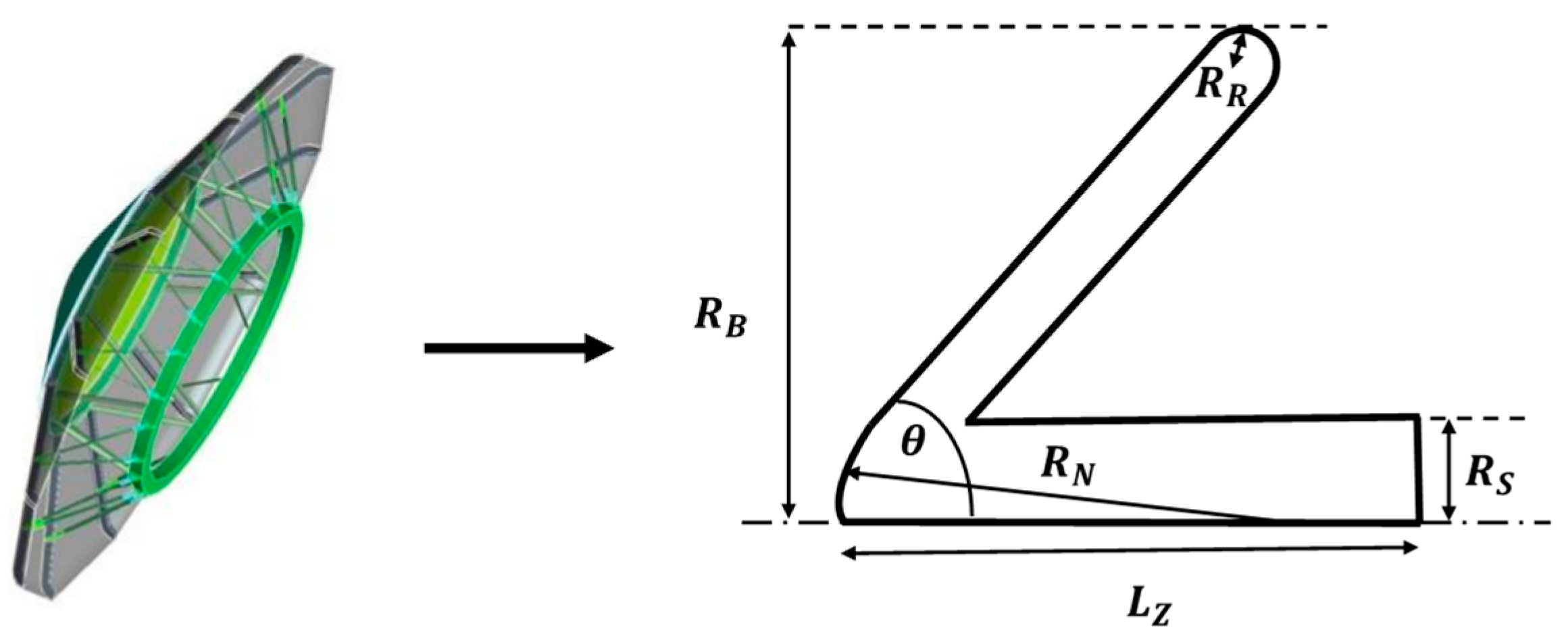
3.1. Geometric Modeling

Based on the shape of the ADEPT model [6], the parametric diagram of the mechanical expanded reentry vehicle is shown in Figure 3. The initial values of the structural and flight parameters are shown in Table 1.

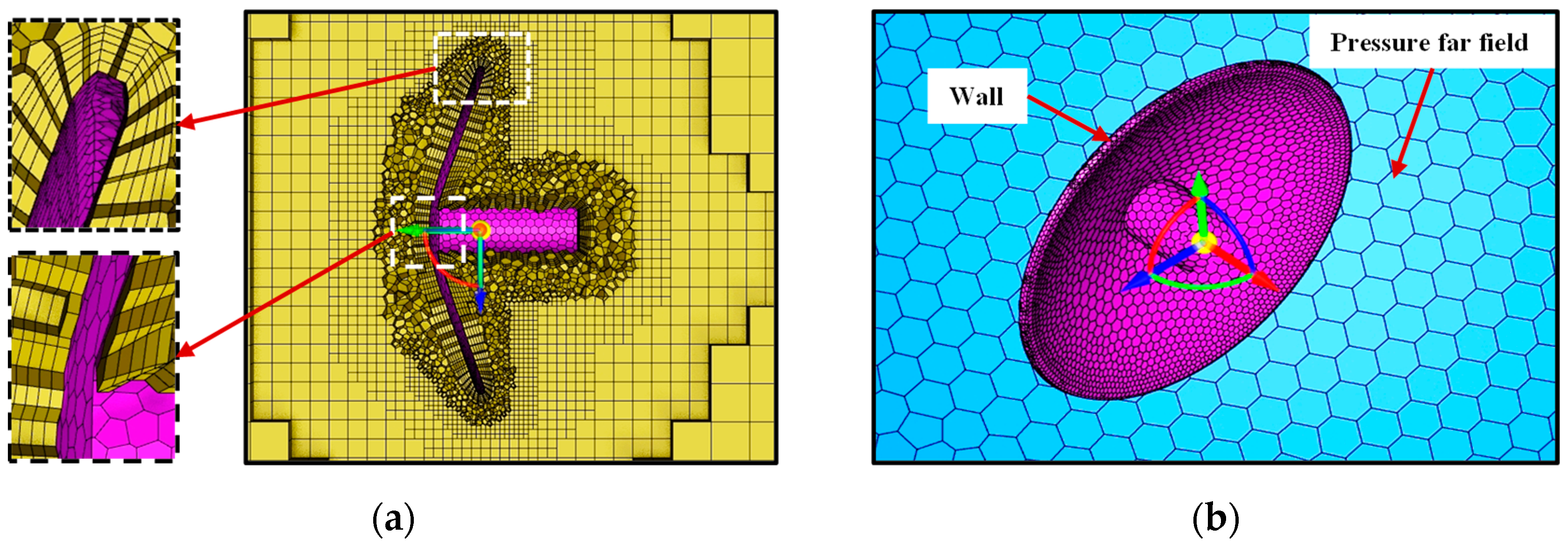
3.2. Mesh Model and Boundary Conditions

The 3D model of the reentry vehicle was established in Figure 4 with the initial structural parameters in Table 1. The unstructured hexagonal surface mesh and hybrid volume mesh were used for grid division, and the boundary layer mesh the near wall of the vehicle was encrypted, as shown in Figure 5a. The vehicle surface was set as a constant temperature wall without slip. The pressure far field was selected as the boundary condition [9], as shown in Figure 5b. The freestream condition is presented in Table 2.

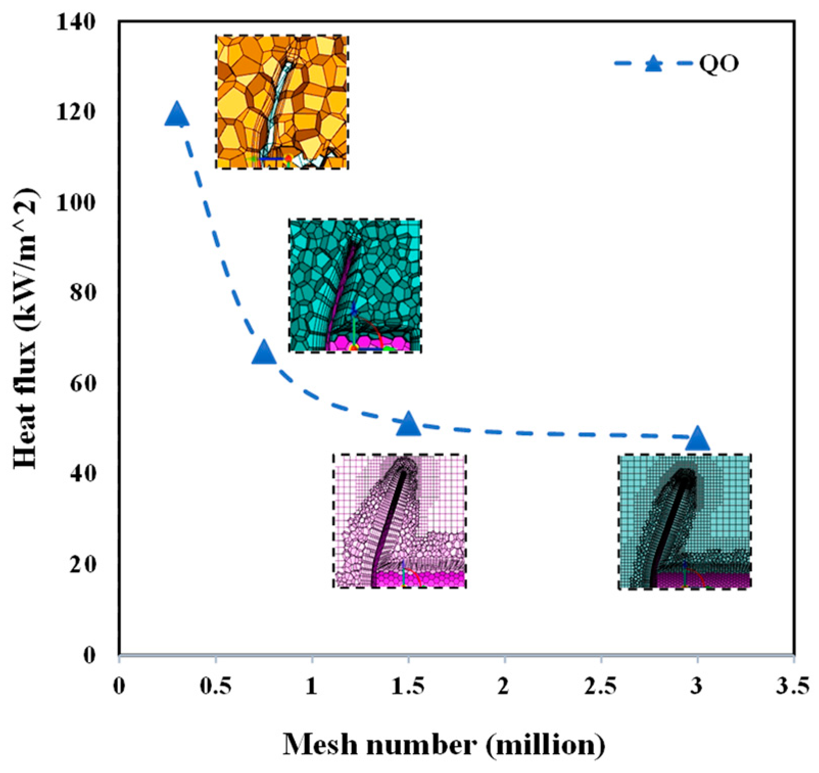
3.3. Mesh Independence Verification

The number of mesh has a significant influence on the calculation accuracy and calculation consumption [36]. The mesh independence is verified by the heat flux QO at stagnation point. Using the initial shape in Figure 4 and the freestream conditions in Table 2, the number of mesh ranges from 0.3 million to 3 million. The calculation comparison results are shown in Table 3 and Figure 6. When the number of the mesh is larger than 1.5 million, the value QO tends to be constant. Finally, the flow field mesh number is determined to be about 1.5 million for calculation.

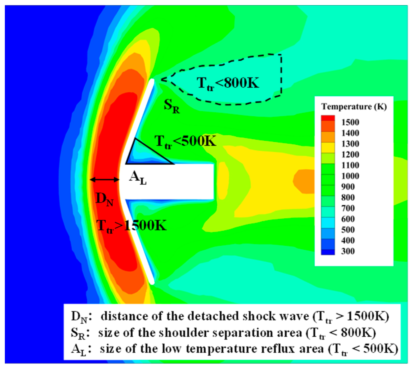
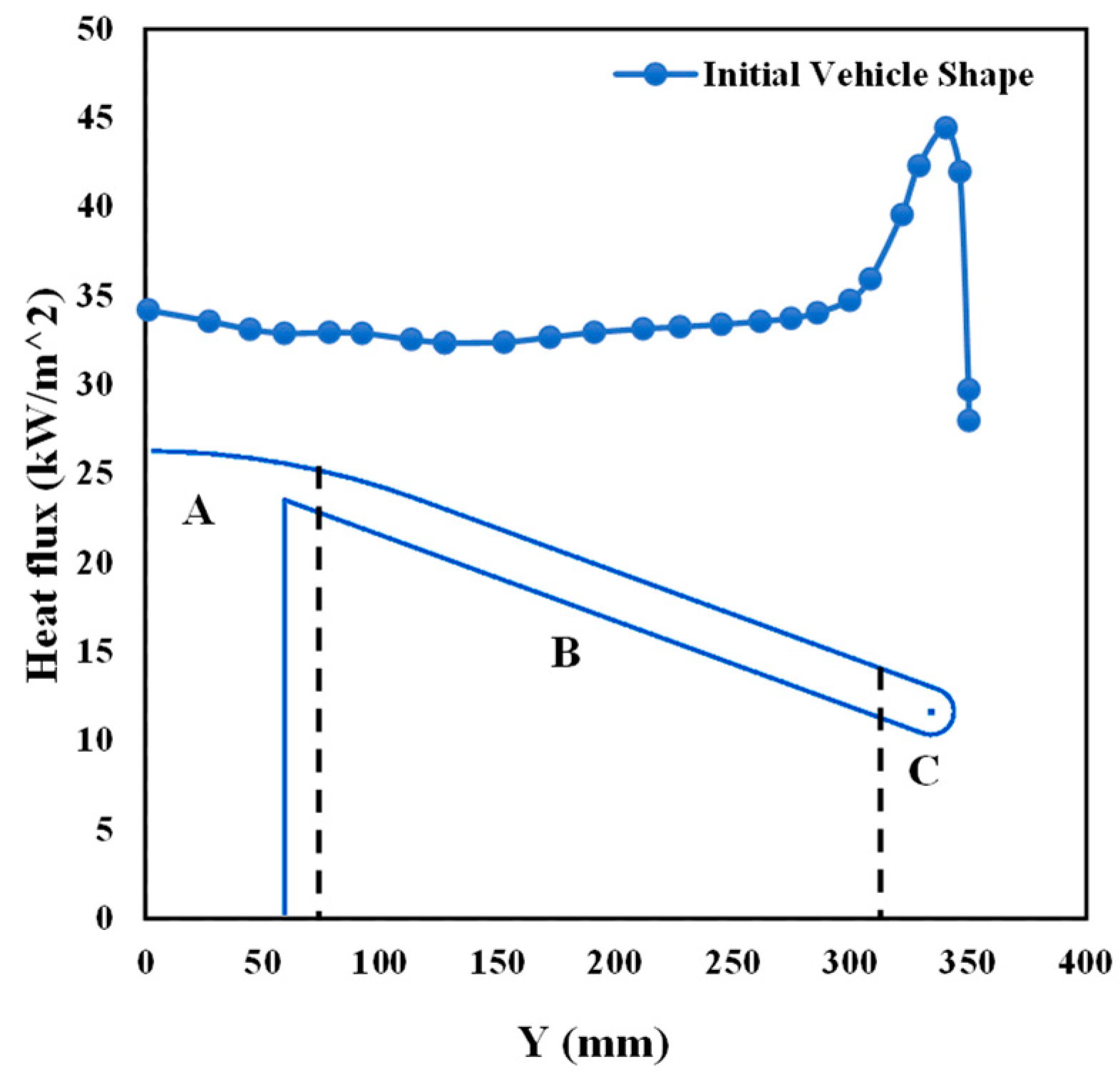
3.4. Simulation Results and Analysis of Initial Condition

The initial shape and working conditions in Table 1 and Table 2 are used for simulation, and the flow field of the Two-Temperature model is obtained as shown in Figure 7 above. The left contour is based on the translational rotation temperature (Ttr), which represent translational and rotational energy change. The right one shows the vibratory electron temperature (Tve) calculated by the transport equation of vibrating electrons in Section 2.1. From these two contours, the change of the flow field is shown more clearly.
The flow field is divided into three regions (A/B/C) as explained in Figure 7a. In region A, the detached shock wave is formed before the head of the vehicle. Ttr in this region is higher than the other regions because the incoming air is heated strongly after passing through the shock wave. In region B, Ttr drops in gradient on the vehicle surface, but not appreciably. Then, in region C, a rapid flow separation occurs at the shoulder. Ttr has a large gradient increase, and the flow is more complex. Combined with Tve, there is also a separation in region C, with Tve increasing obviously at the shoulder. This shows that the incoming air expands rapidly in region C and increases the aerodynamic heating.
To further characterize the flow field details of the reentry vehicle, three characteristic parameters shown in Figure 8 were chosen to compare and analyze the temperature contours. These exist in the stagnation point region of Ttr > 1500 K. SR shows the size of the shoulder separation area where Ttr < 800 K. AL denotes the size of the low temperature reflux area, which is close to the wall and Ttr < 500 K. These three characteristic parameters are different in different cases of flow fields, and their variation trend can help analyze the flow field and heat flux changes.
The results of heat flux distribution along the Y direction are shown in Figure 9. The heat flux at stagnation region is about 34 kW/m2. A lot of kinetic energy is converted to heat energy at stagnation point. After leaving the stagnation point, the heat flux gradually decreases until near the shoulder region. When the air flow passes through the shoulder, the expansion wave generated by the flow separation plays a leading role, which makes the air velocity increase. According to the Fourier heat transfer law, when the fluid velocity increases, the heat transfer capacity also increases, and it is greater than its ability to cool down. Therefore, the heat flux suddenly increases to 44 kW/m2. After passing the shoulder, it reduces to a lower value.
In the initial configuration and flight condition, the heat flux of the shoulder point QR is greater than the heat flux at stagnation point QO, which is contrary to the previous belief that the heat flux at the stagnation point is the maximum. Therefore, it is necessary to study in detail the variation trend of the surface heat flux and the distribution law of the maximum heat flux point under different structural parameters and flight conditions.

4. Results and Analysis of Different Structural and Flight Parameters

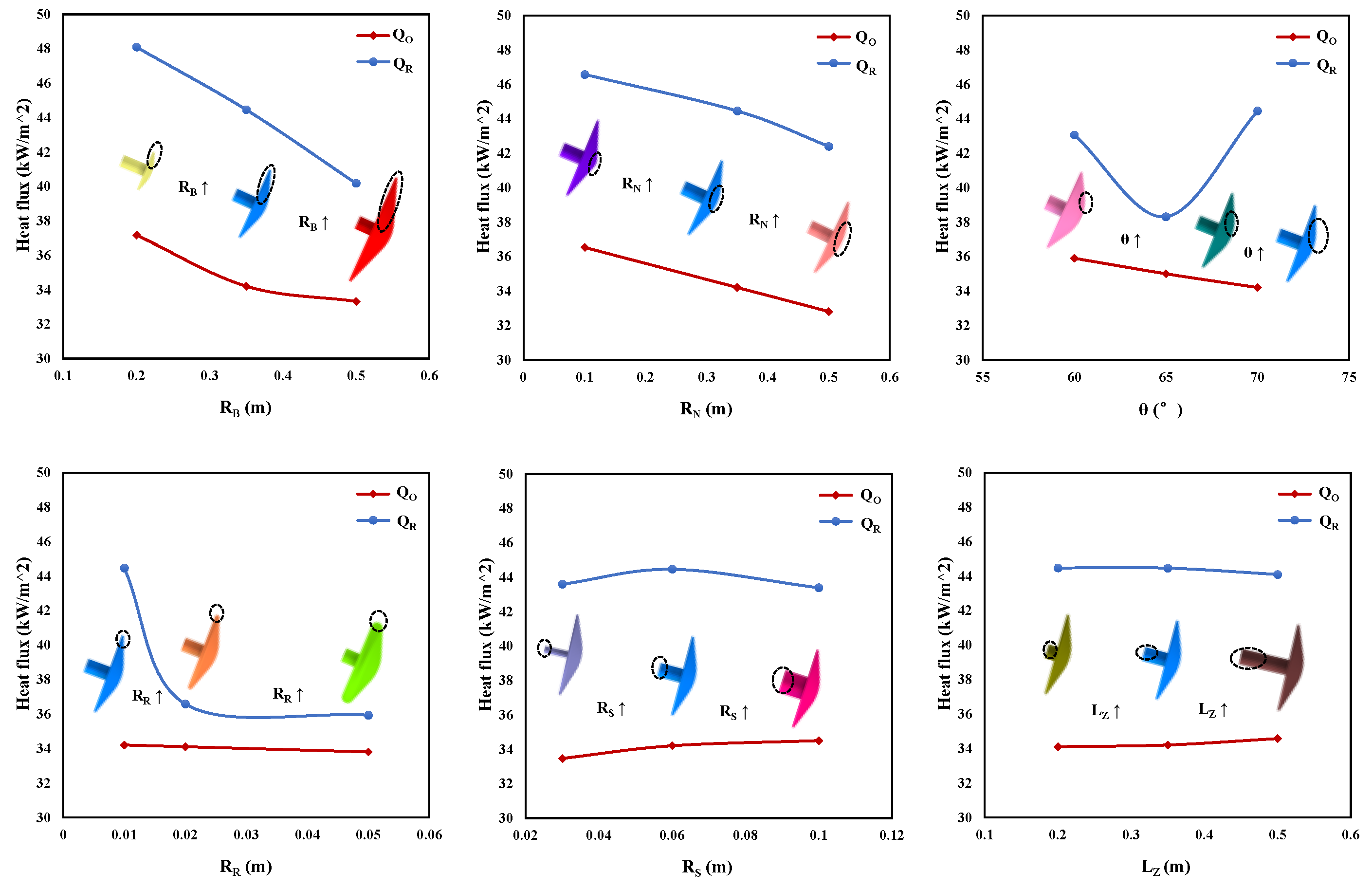
4.1. Influence of Different Structural Parameters

Structural parameters are important factors affecting the flow field and surface heat flux distribution. Six structural parameters from ADEPT were selected in this paper, including expansion radius RB, nose cone radius RN, half cone angle θ, shoulder radius RR, base radius RS, and total length LZ. Flight parameters were selected in Table 1. The influence of different structural parameters on the flow field and heat flux distribution was explored using the following cases shown in Table 4.

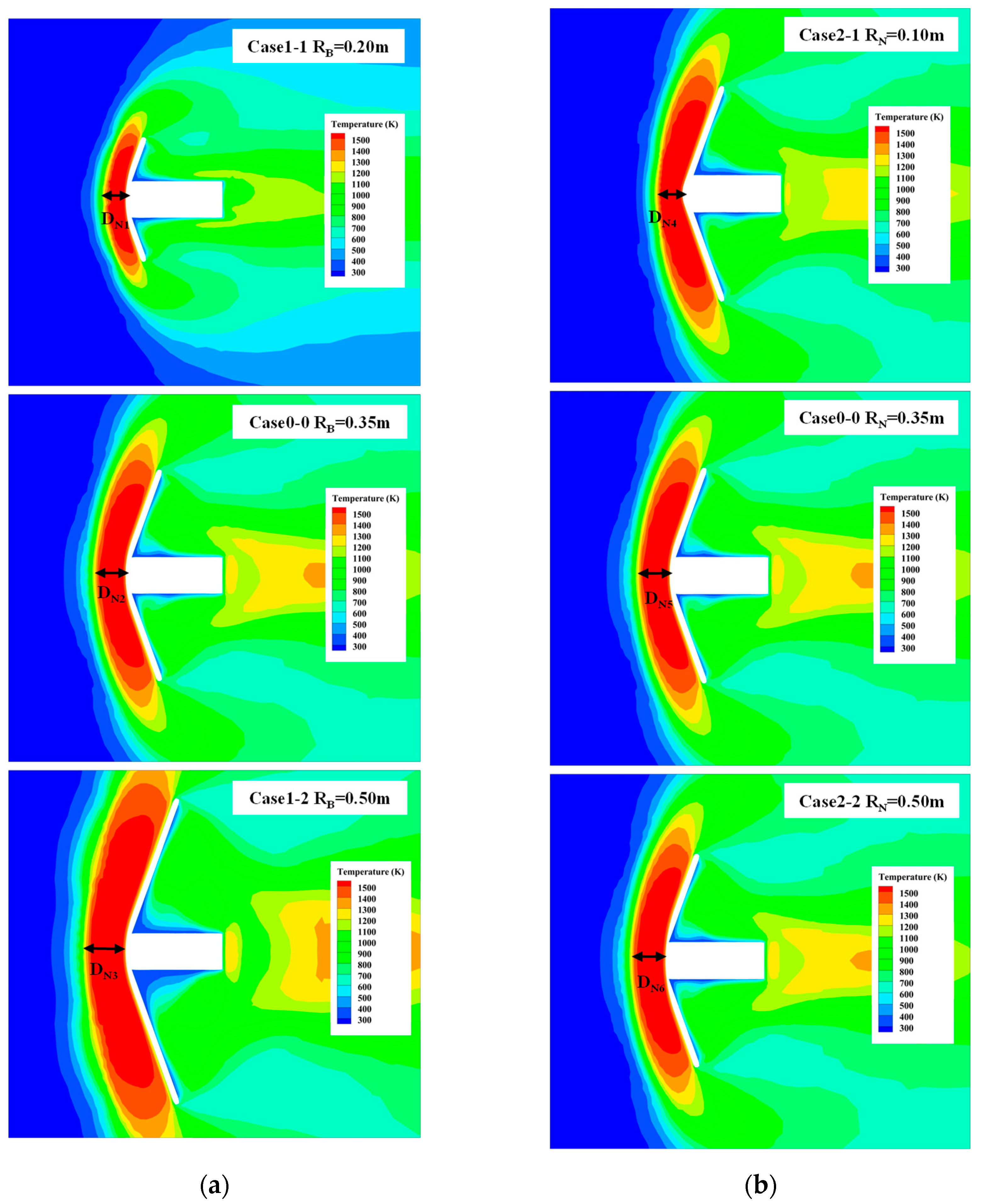
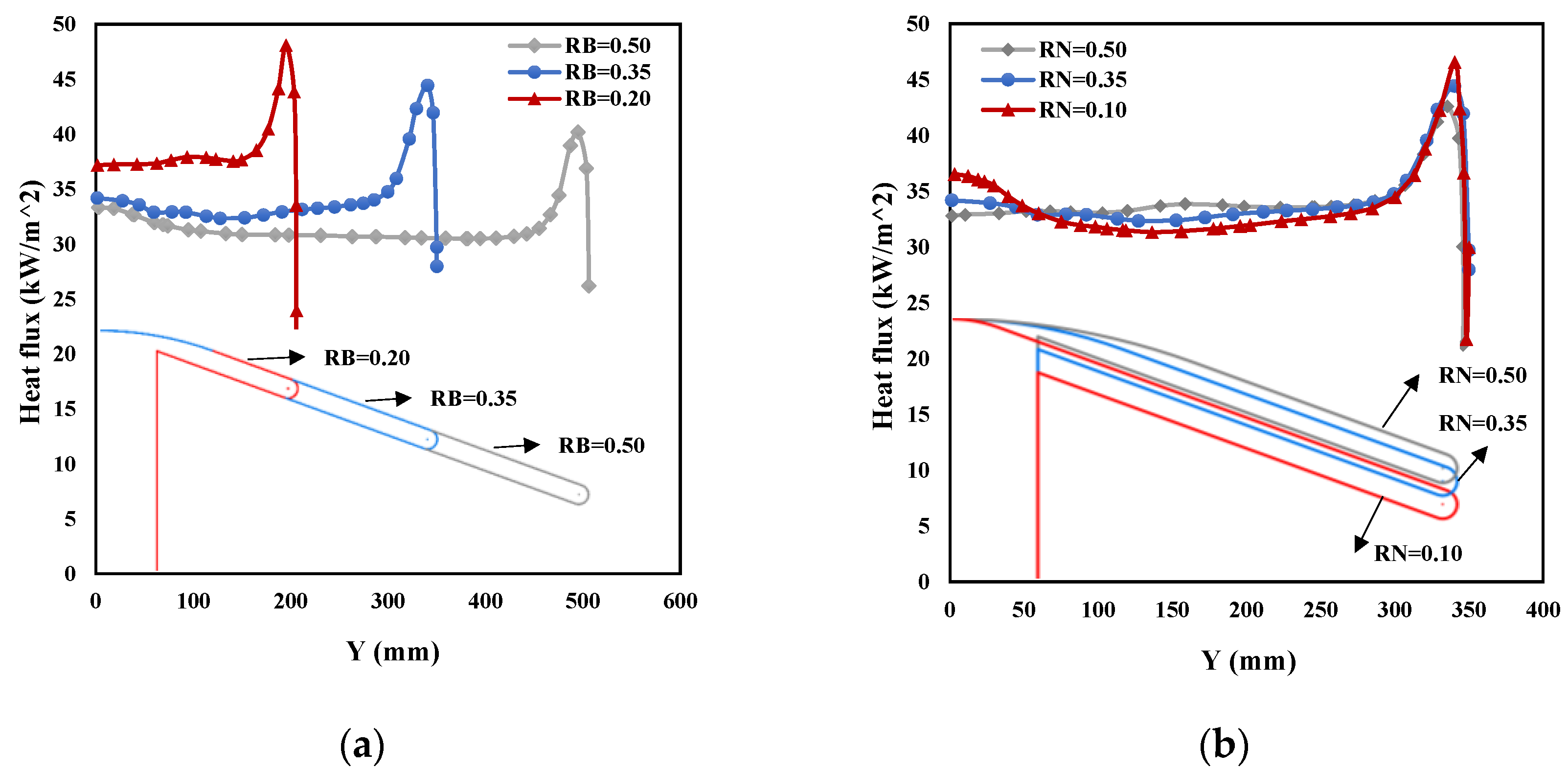
4.1.1. Influence of RB and RN

Figure 10 shows the temperature contours after changing RB and RN. In the stagnation region, the temperature gradient changes in the same trend when RB gradually increases; however, the distance of the detached shock wave DN increases with an increase in RB. When RN changes from small to large, the dullness of the vehicle head enhances, which also makes DN gradually increase. In the thick shock layer, the air translative temperature rises slowly, and the heat exchange between the air molecules and the wall decreases, resulting in a decrease in aerodynamic heating in the stagnation region. Therefore, the aerodynamic heating can be effectively reduced by adjusting the structural parameters and by reasonably controlling DN.
The heat flux distribution with different RB and RN are shown in Figure 11; when only RB and RN change, the heat flux of the shoulder QR is always larger than that of the stagnation point QO. QO and QR decrease when RB increases. When RN changes from large to small, QO and QR increase respectively; however, the difference value between QO and QR remains unchanged. Therefore, the heat flux of the vehicle can be decreased by increasing RB and RN.

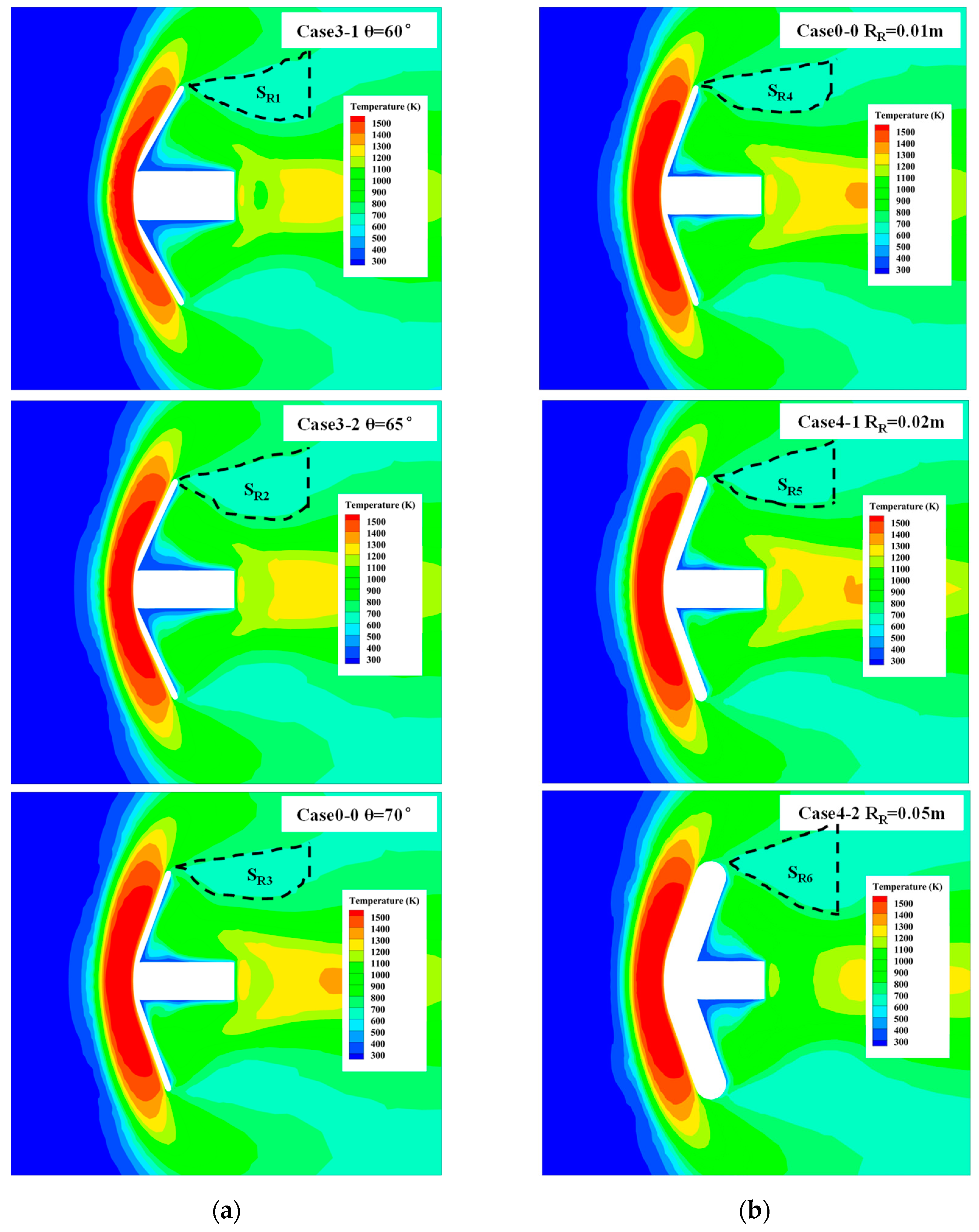
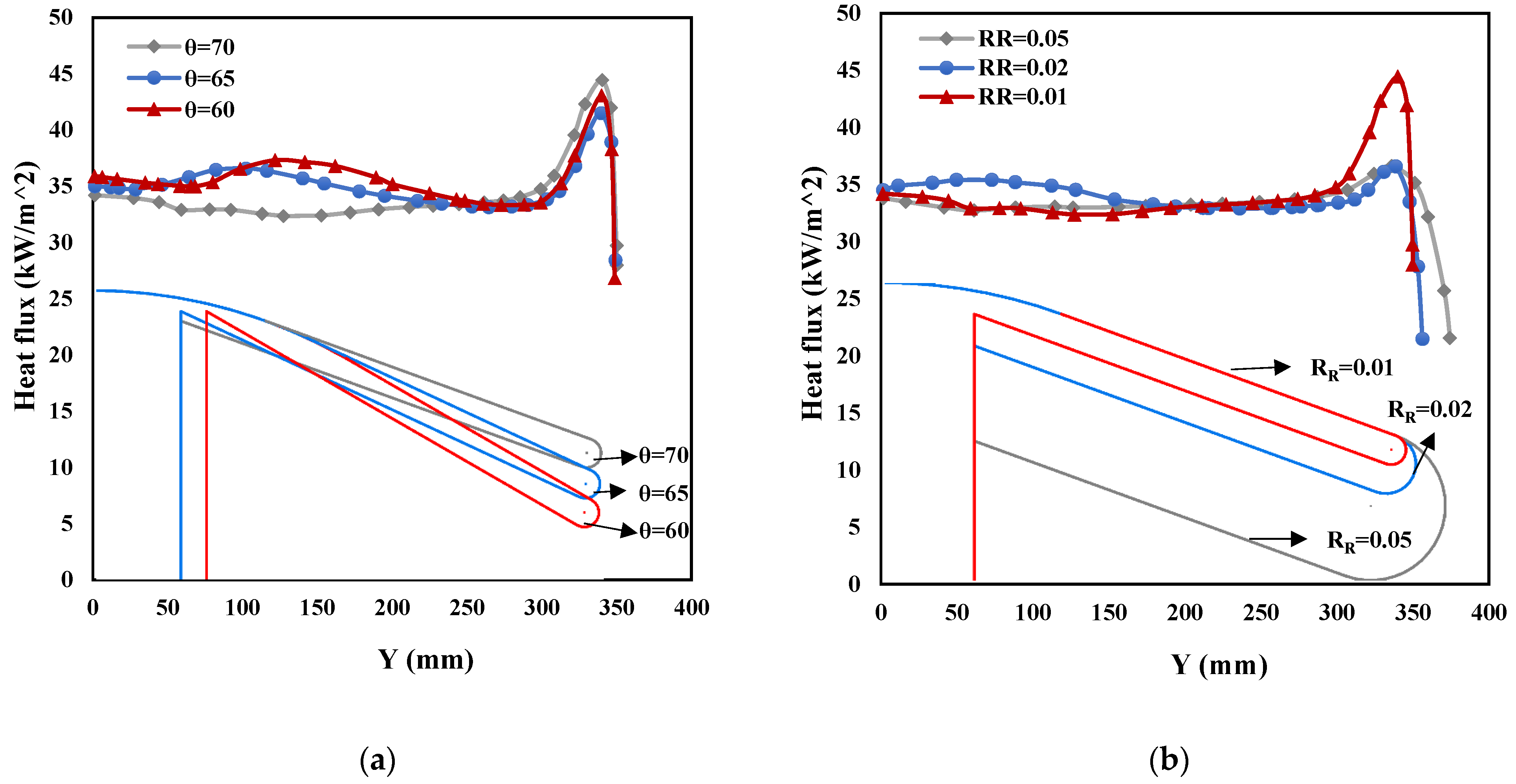
4.1.2. Influence of θ and RR

Temperature contours after changing θ and RR are shown in Figure 12. When θ and RR change, the structure of the flow field changes a little at stagnation point but significantly at the shoulder point. SR is one of the important field characters which can evaluate the effect of shoulder flow separation. Combined with Figure 7b above, in the separation area, incoming air expands rapidly and results in flow separation. When Ttr > 800 K, the vibrational energy of the gas in the expansion layer is excited. When SR is small, the region of Ttr > 800 K is larger, and more gas molecules are excited. Moreover, the energy also increases the aerodynamic heating, leading to peak values at the shoulder. SR drops first and then rises from case 3-1 to case 3-3. It becomes largest when θ = 65° and when the heat flux peak value is smallest. When RR increases, SR increases, and the heat flux peak value declines continuously. Therefore, a large SR is expected to reduce the heat flux at the shoulder point.
Figure 13 shows the heat flux distribution when θ and RR change. The change in the half cone angle θ affects the position of the shoulder point relative to the stagnation point. With θ increasing, the shoulder point is closer to the stagnation point; however, this change has little influence on QO. QR has the smallest value when θ = 65°. The influence of shoulder radius RR on QR is more obvious. When RR increases from 0.01 m to 0.02 m, QR decreases significantly by 18%; when RR increases from 0.02 m to 0.05 m, the change is small, and QO is very close to QR in this case. The position of the peak heat flux point jumps with a change in RR. The peak heat flux should be accurately estimated to complete the design of the whole thermal protection system.

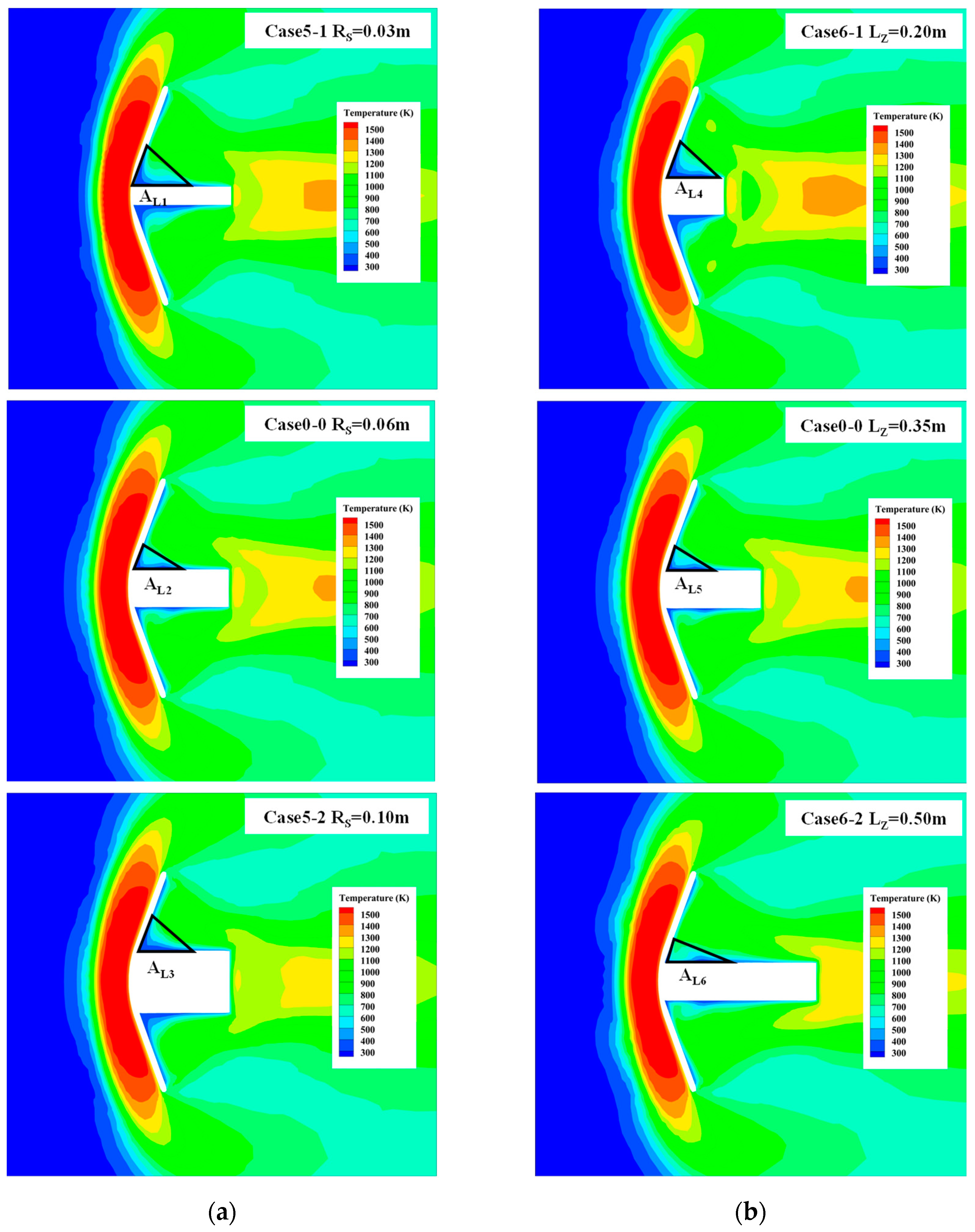
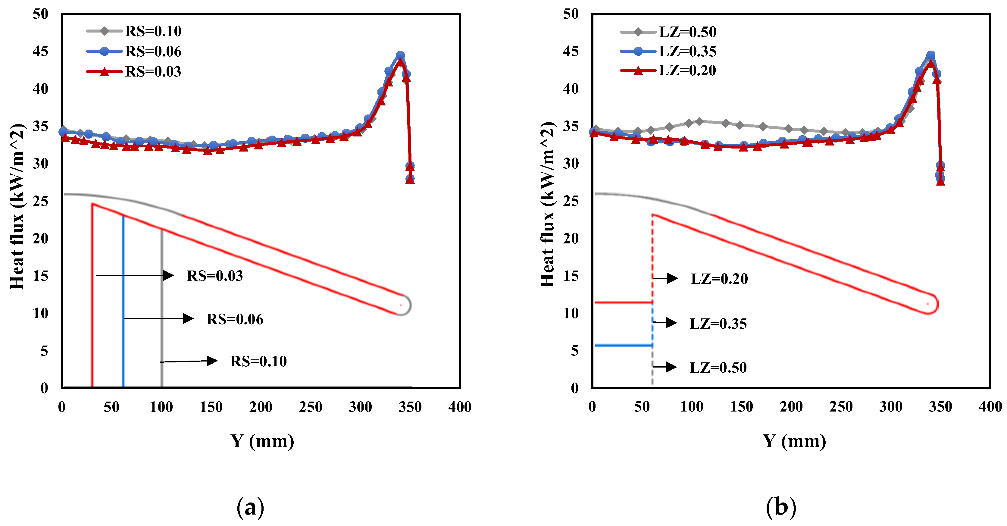
4.1.3. Influence of RS and LZ

Temperature contours after changing the other two structural parameters RS and LZ are shown in Figure 14. They have no obviously direct influence on the complex flow field in the stagnation region and shoulder region; however, in surface area, AL represents the size of the low temperature reflux area where Ttr < 500 K; moreover, it also affects the heat flux distribution. The heat transfer effect of gas decreases at low temperature. When AL is large, the heat flux on the surface region of the vehicle will decrease slightly. AL decreases first and then increases when the base radius RS gradually increases. At the same time, increasing the total length LZ will continuously decrease AL. Increasing AL can also contribute to a reduction in aerodynamic heating.
It can be seen from Figure 15 that changing RS and LZ has little effect on the distribution of the surface heat flux. Moreover, the value of QO and QR changes little. It is worth mentioning that, when LZ increases to 0.50 m, the heat flux between the stagnation point and shoulder point is larger than that with the small LZ. This may be related to the length no longer causing the delay of the low temperature reflux area. RS and LZ have little influence on the surface heat flux.

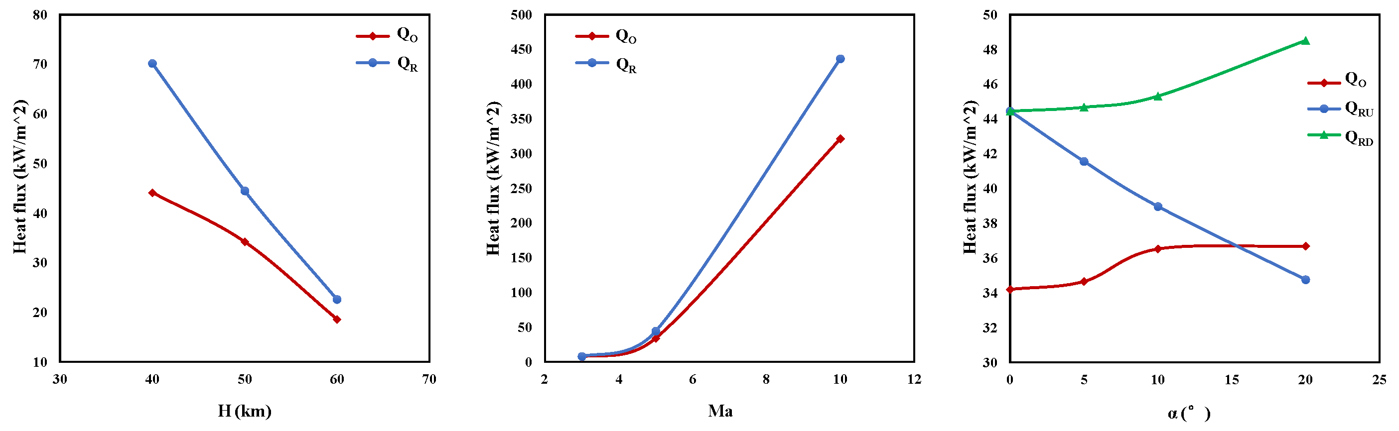
4.2. Influence of Different Flight Parameters

Different flight conditions also have a significant influence on the flow field structure and surface heat flux distribution. The flight altitude H, flight Mach number Ma, and flight attack angle α are changed to explore the influence in this study. The shape parameters are set as constant, as shown in Table 1. The variation of flight parameters used for simulation are shown in Table 5.

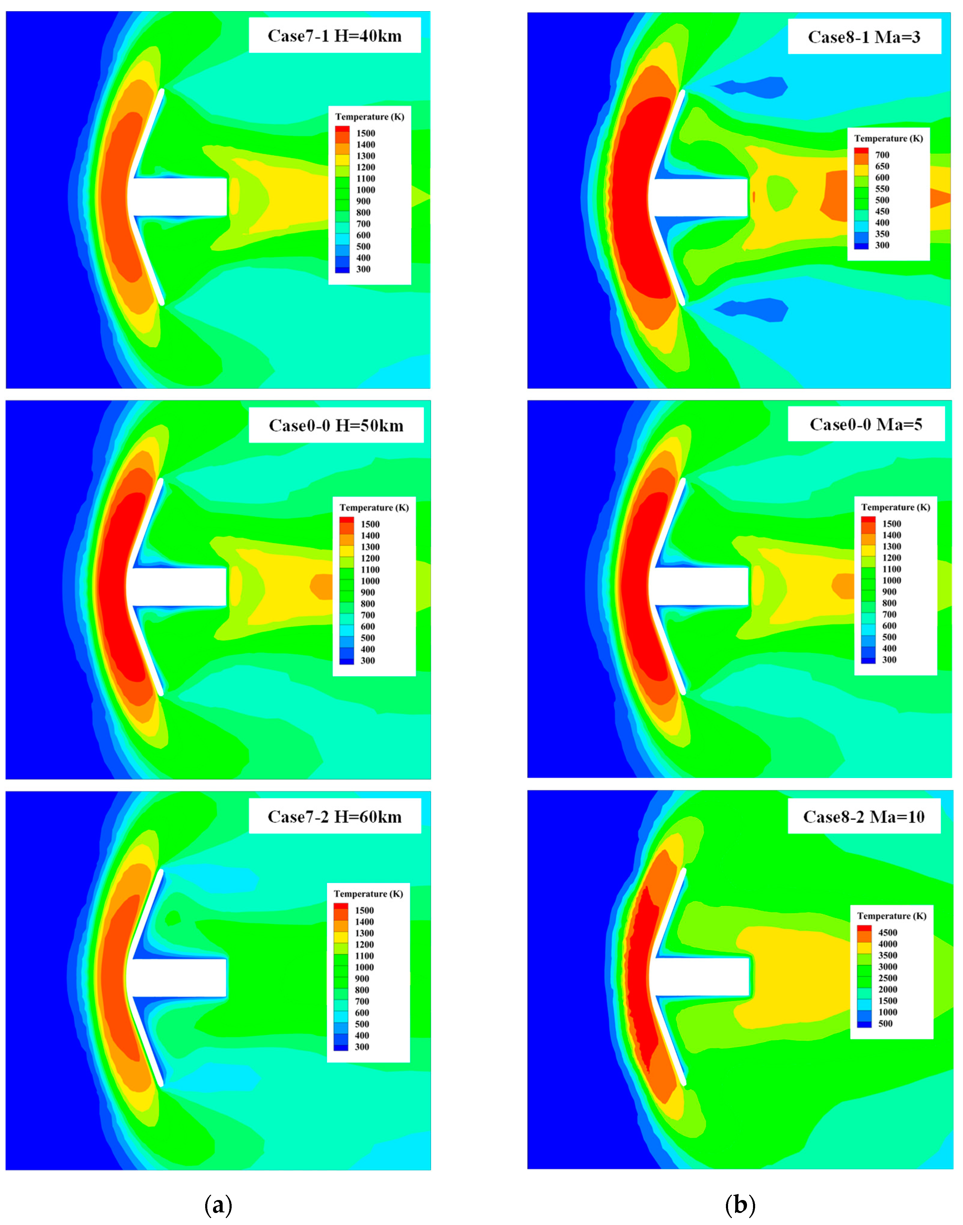
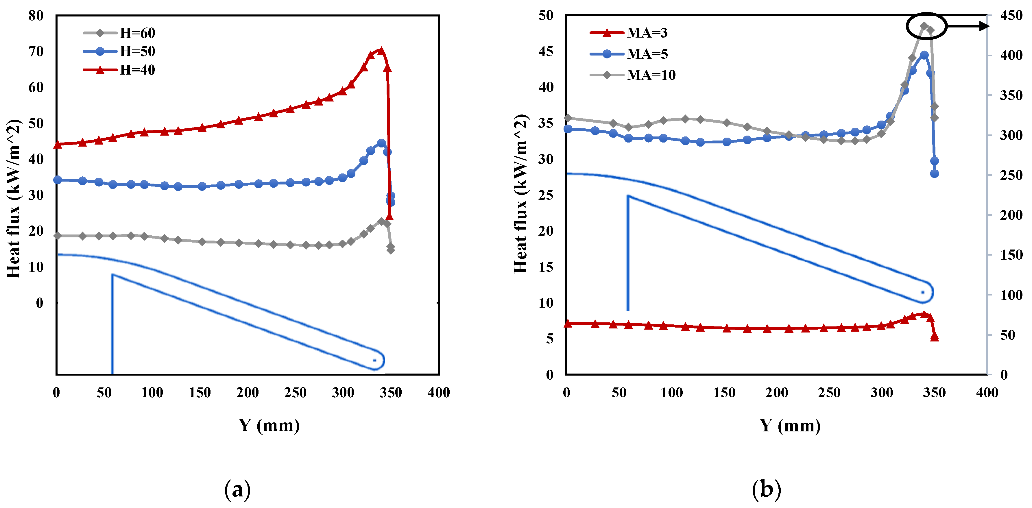
4.2.1. Influence of H and Ma

Figure 16 shows the temperature contours when H and Ma change. When the flight altitude H is between 40 km and 60 km, as it rises, the air density gradually decreases, and the aerodynamic heating also decreases. Ma is an important factor affecting aerodynamic heating. The temperature and aerodynamic heating increase obviously when Ma increases. When the temperature exceeds 2500 K, it is necessary to consider the air dissociation mechanism in the CFD simulation. In case 8-2, the chemical reaction considering five gas components, excluding atomic ionization via the Gupta model, was chosen to reflect air dissociation in the simulation. The 10 Ma hypersonic incoming flow generates a high temperature of over 4000 K near the stagnation point of the vehicle, resulting in a very dangerous thermal environment.
Heat flux distribution of changing H and Ma are shown in Figure 17 After the flight altitude of H changes, due to the obvious change in air density, the surface heat flux of the vehicle also changes significantly. The overall heat flux distribution decreases with an increase in H. When H = 40 km and Ma = 5, QR reaches 70 kW/m2 at the shoulder point. With an increase in Ma, aerodynamic heating is enhanced significantly. QR reaches 380 kW/m2, which is far beyond the thermal protection limits of ordinary materials when Ma = 10. Therefore, it is necessary to reduce speed at a lower altitude to reduce aerodynamic heating as much as possible.

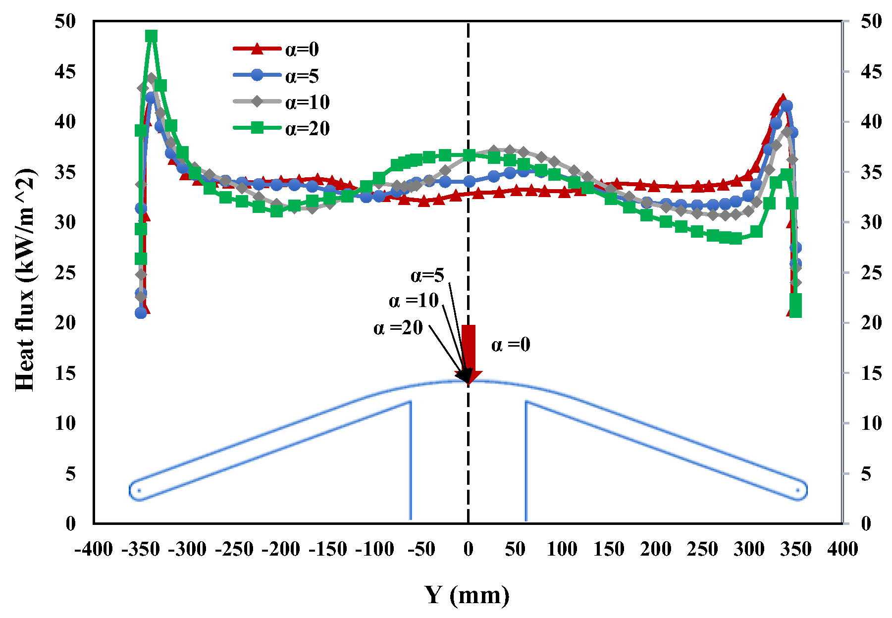
4.2.2. Influence of α

Figure 18 shows the temperature contours of case 0-0 and 9-1 to 9-3. During the reentry process with the attack angle α, the aerodynamic heating of the vehicle via the incoming air will not be symmetrical. With an increase in α, the deuterated shock wave near the stagnation point concentrates in the part opposite the incoming air, and the air expansion and separation in the down shoulder area are more obvious. The low temperature reflux area converges in the opposite air part. Therefore, aerodynamic heating mainly occurs in the shoulder region, which is opposite the incoming air, while the thermal environment of the other shoulder region is relatively mild.
The heat flux distribution of different attack angle α is shown in Figure 19. The heat flux is asymmetrically distributed on the vehicle surface as α changes. QRD means the heat flux of the down shoulder part where Y < 0 while QRU represents the heat flux at the shoulder of the Y > 0 part. When α increases, QRD keeps increasing, while QRU keeps decreasing, resulting in more heating at one part. As α increases, the heat flux difference between the two parts also increases. Therefore, when there is an attack angle flight, it is necessary to accurately calculate the heat flux distribution and thermally protect the vehicle shoulder point.

4.3. Summary of Influence

Based on the above analysis, the influence law of different structural and flight parameters on the surface heat flux of the vehicle has been obtained. Structural parameters affect the heat flux values of the stagnation point and shoulder point by changing the flow field structure such as DN, SR, and AL. Figure 20 shows the variation trend of QO and QR with structural parameters. The change in the aerodynamic shape brought by the change in structural parameters is also reflected.
In the simulation of the selected sample points, QR has been always larger than QO, which means the heat flux peak value occurs at the shoulder of the vehicle. RB, RN, and θ have an obviously negative effect on QO, and the other three parameters have little effect. RB, RN, RR, and LZ have a negative correlation with QR. The effect of θ and RS on QR become more complex: QR drops first and then rises as θ increases; when RS increases, QR increases first and then decreases. It is worth noting that increasing RR significantly reduces QR; however, up to a certain point, QR does not reduce anymore.
Figure 21 shows the variation trend of QO and QR with flight parameters H, Ma, and α. The flight parameters directly and significantly affect QO and QR, in which Ma is positive and H is negative. The attack angle α occurs to produce a different value of QR; moreover, increasing α will increase QO and QRD while reducing QRU. QO will be larger than QRU but also smaller than QRD at a high angle of attack. Through our analysis, the design goal of the heat flux minimum value can be achieved by adjusting the structural and flight parameters.

5. Conclusions

This paper adopts a Two-Temperature model using the CFD numerical method to simulate the flow field structure of a mechanical expanded reentry vehicle to study the heat flux distribution of the vehicle surface. Some conclusions are obtained as follows:
(1) The Two-Temperature model for simulation can fully consider the vibration motion processes of electrons during hypersonic reentry. The simulation shows that the calculation results of the Two-temperature model are closer to the flight test. The prediction accuracy can be obviously improved to reflect a real flight situation;
(2) The peak heat flux point may occur at the stagnation point or at the shoulder point, which is different from the traditional conclusion that the stagnation point heat flux is maximum. When the air flow passes through the shoulder, the expansion wave makes the air velocity increase. The heat transfer capacity also increases and is greater than its ability to cool down. The heat flux appears at peak value at the shoulder. Both structural parameters and flight parameters affect the peak heat flux point;
(3) Among the structural parameters, RB, RN, and θ have an obviously negative effect on QO, while the other three parameters cause little effect. RB, RN, RR, and LZ have a negative correlation with QR. QR decreases first and then rises as θ increases and RS decreases. Among the flight parameters, Ma is positive and H is negative. α makes the heat flux distribution asymmetric. Increasing α improves QRD and reduces QRU.

Author Contributions

Conceptualization, H.Z. and D.X.; methodology, J.S. and H.Z.; software, J.S. and H.Z.; validation, J.S. and D.X.; formal analysis, D.X. and G.C.; investigation, H.Z.; resources, G.C.; data curation, D.X.; writing—original draft preparation, J.S. and H.Z.; writing—review and editing, J.S. and D.X.; visualization, J.S.; supervision, G.C.; project administration, D.X. and G.C. All authors have read and agreed to the published version of the manuscript.

Funding

This research was funded by the Fundamental Research Funds for the Central Universities.

Data Availability Statement

Not applicable.

Conflicts of Interest

The authors declare no conflict of interest.

References

  1. Gao, S.; Huang, W. Achievements and prospects of China’s spacecraft recovery and landing Technology in the past 60 years. Space Return Remote Sens. 2018, 39, 70–78. [Google Scholar]
  2. Otsu, H. Aerodynamic Characteristics of Re-Entry Capsules with Hyperbolic Contours. Aerospace 2021, 8, 287. [Google Scholar] [CrossRef]
  3. Zhang, P.; Li, X.; Bai, L.; Shang, M.; Zhang, H.; Hou, X. Review of Expanded Pneumatic Deceleration Technology for Semi-rigid Machinery. Space Return Remote Sens. 2016, 37, 1–9. [Google Scholar]
  4. Friz, P.D. Parametric Cost Estimates of Four 20 Ton Payload Mars EDL Vehicle Concepts. In Proceedings of the AIAA Scitech 2020 Forum, Orlando, FL, USA, 6–10 January 2020. [Google Scholar]
  5. D’Souza, S.N.; Okolo, W.; Nikaido, B.; Yount, B.; Tran, J.; Margolis, B.; Smith, B.; Cassell, A.; Johnson, B.; Hibbard, K.; et al. Developing an Entry Guidance and Control Design Capability Using Flaps for the Lifting Nano-ADEPT. In Proceedings of the AIAA Aviation 2019 Forum, Dallas, TX, USA, 17–21 June 2019. [Google Scholar]
  6. Saranathan, H.; Saikia, S.; Grant, M.J.; Longuski, J.M. Trajectory Optimization with Adaptive Deployable Entry and Placement Technology Architecture. In Proceedings of the 11th International Planetary Probe Workshop, Pasadena, CA, USA, 16–20 June 2014. [Google Scholar]
  7. Wercinski, P.; Smith, B.; Battazzo, Y.; Kruger, C.; Brivkalns, C.; Makino, A.; Cassell, A.; Dutta, S.; Ghassemi, S. ADEPT sounding rocket one (SR-1) flight experiment overview. In Proceedings of the 2017 IEEE Aerospace Conference, Big Sky, MT, USA, 4–11 March 2017. [Google Scholar]
  8. O’Driscoll, D.S.; Bruce, P.J.K.; Santer, M. Design and Dynamic Analysis of Rigid Foldable Aeroshells for Atmospheric Entry. J. Spacecr. Rocket. 2021, 58, 741–753. [Google Scholar] [CrossRef]
  9. Smith, B.; Venkatapathy, E.; Wercinski, P.; Yount, B.; Prabhu, D.; Gage, P.; Glaze, L.; Baker, C. Venus In Situ Explorer Mission design using a mechanically deployed aerodynamic decelerator. In Proceedings of the IEEE Aerospace Conference, Big Sky, MT, USA, 2–9 March 2013. [Google Scholar]
  10. Yang, X.; Wang, J.; Zhou, Y.; Sun, K. Assessment of Radiative Heating for Hypersonic Earth Reentry Using Nongray Step Models. Aerospace 2022, 9, 219. [Google Scholar] [CrossRef]
  11. Saikia, S.J.; Saranathan, H.; Grant, M.J.; Longuskiet, J.M. Trajectory optimization for adaptive deployable entry and placement technology (ADEPT). In Proceedings of the Astrodynamics Specialist Conferences, San Diego, CA, USA, 4–7 August 2014. [Google Scholar]
  12. Griffin, M.D.; French, J.R. Space Vehicle Design, 2nd ed.; American Institute of Aeronautics & Astronautics: Reston, VA, USA, 2004; Volume 279. [Google Scholar] [CrossRef]
  13. Zhang, S.; Yu, L.; Cao, X.; Zhang, Z. Prediction method of peak Thermal Load for reentry returner. Aerosp. Return Remote Sens. 2019, 40, 25–32. [Google Scholar]
  14. Zhang, M. Numerical Simulation of Aero-Thermal Environment for Earth Re-Entry/Outer Planet Entry Vehicle. Master’s Thesis, Shandong University, Jinan, China, 2017. [Google Scholar]
  15. Liu, F.; Yuan, J. Discussion on the calculation formula of stagnation heat flow in non-equilibrium Martian atmosphere. Manned Spacefl. 2018, 24, 582–589. [Google Scholar]
  16. Hergert, J.; Brock, J.; Stern, E. Free-Flight Trajectory Simulation of the ADEPT Sounding Rocket Test Using US3D. In Proceedings of the 35th AIAA Applied Aerodynamics Conference, Denver, CO, USA, 5–9 June 2017. [Google Scholar]
  17. Viviani, A.; Pezzella, G.; Borrelli, S. Effect of Finite Rate Chemical Models on the Aerothermodynamics of Reentry Capsules. In Proceedings of the 15th Proceeding of AIAA International Space Planes and Hypersonic Systems and Technologies Conference, Dayton, OH, USA, 28 April–1 May 2008. [Google Scholar]
  18. Alkandry, H.; Boyd, D. Numerical Study of Hypersonic Wind Tunnel Experiments for Mars Entry Aeroshells. In Proceedings of the 41th Thermophysics Conference, San Antonio, TX, USA, 22–25 June 2009. [Google Scholar]
  19. Bisceglia, S.; Ranuzzi, G. Real Gas Effects on a Planetary Reentry Capsule. In Proceedings of the 13th AIAA/CIRA International Space Planes and Hypersonics Systems and Technologies, Capua, Italy, 16–20 May 2005. [Google Scholar]
  20. Maciel, E. Three-Temperature Model Applied to Thermochemical Non-Equilibrium Reentry Flows in 2D—Seven Species. Fluid Dyn. 2022, 12, 35. [Google Scholar]
  21. Viviani, A.; Golia, C.; Pezzella, G. Analysis of thermochemical modeling and surface catalyticity in space vehicles reentry. In Proceedings of the International Congress of The Aeronautical Sciences, Anchorage, AK, USA, 14–19 September 2008. [Google Scholar]
  22. Liu, M. Numerical Simulation of Apollo-Like Re-Entry Vehicle. Master’s Thesis, Harbin Institute of Technology, Harbin, China, 2014. [Google Scholar]
  23. Matsunaga, M.; Takahashi, Y.; Oshima, N.; Yamada, K. Aerodynamic Heating Prediction of an Inflatable Reentry Vehicle in a Hypersonic Wind Tunnel. In Proceedings of the 55th AIAA Aerospace Sciences Meeting, Grapevine, TX, USA, 9–13 January 2017; American Institute of Aeronautics and Astronautics: Reston, VA, USA, 2017. [Google Scholar]
  24. Dejarnette, F.R.; Hamilton, H.H.; Weilmuenster, K.J.; Cheatwood, F.M. A Review of Some Approxmate Methods Used in Aerodynamic Heating Analyses. J. Thermophys. Heat Transf. 1987, 1, 5–12. [Google Scholar] [CrossRef]
  25. Kimmel, R.L.; Adamczak, D.W. HIFiRE-1 flight trajectory estimation and initial experimental results. In Proceedings of the 17th AIAA International Space Planes and Hypersonic Systems and Technologies Conference, San Francisco, CA, USA, 11–14 April 2011; AIAA: Reston, VA, USA, 2011. [Google Scholar]
  26. Spalart, P.; Allmaras, S. A one-equation turbulence model for aerodynamic flows. In Proceedings of the 30th Aerospace Sciences Meeting and Exhibit, Reno, NV, USA, 6–9 January 1992. [Google Scholar]
  27. Shih, T.H.; Liou, W.W.; Shabbir, A.; Yang, Z.; Zhu, J.A. A new k-e eddy viscosity model for high Reynolds number turbulent flows. Comput. Fluids 1995, 24, 227–238. [Google Scholar] [CrossRef]
  28. Ocokoljic, G.; Rasuo, B.; Kozic, M. Supporting system interference onaerodynamic characteristics of an aircraft model in a low-speed wind tunnelAerosp. Sci. Technol. 2017, 64, 133–146. [Google Scholar]
  29. Wilcox, D.C. Turbulence modeling for CFD: DCW industries La Canada. Ca DCW Ind. 1998, 2, 103–217. [Google Scholar]
  30. Kimmel, R.L.; Adamczak, D.W. HIFiRE-l preliminary aerothermodynamics measurements. In Proceedings of the 41th AIAA Fluid Dynamics Conference and Exhibit, Honolulu, HI, USA, 27–30 June 2011; AIAA: Reston, VA, USA, 2011. [Google Scholar]
  31. Yentsch, R.J.; Gaitonde, D.V.; Kimmel, R.L. Performance of turbulence modeling in simulation of the HIFiRE-1 flight test. J. Spacecr. Rocket. 2014, 51, 117–127. [Google Scholar] [CrossRef]
  32. Takahashi, Y.; Ha, D.; Yamada, K.; Abe, T. Numerical Simulation of Flow Field around an Inflatable Reentry Vehicle during a Demonstration Flight. In Proceedings of the AIAA Applied Aerodynamics Conference, Atlanta, GA, USA, 16–20 June 2014. [Google Scholar]
  33. Saidi, N.; Cerdoun, M.; Khalfallah, S.; Toufik, B. Numerical investigation of the surface roughness effects on the subsonic flow around a circular cone-cylinder. Aerosp. Sci. Technol. 2020, 107, 106271. [Google Scholar] [CrossRef]
  34. Casseau, V.; Palharini, R.; Scanlon, T.; Brown, R. A Two-Temperature Open-Source CFD Model for Hypersonic Reacting Flows, Part One: Zero-Dimensional Analysis. Aerospace 2016, 3, 34. [Google Scholar] [CrossRef] [Green Version]
  35. Gnoffo, P.A.; Gupta, R.N.; Shinn, J.L. Conservation Equations and Physical Models for Hypersonic Air Flows in Thermal and Chemical Nonequilibrium; NASA: Washington, DC, USA, 1989. [Google Scholar]
  36. Chen, L.; Xia, J. Study on the Leading Edge of a Hypersonic Vehicle Using the Aero-Thermoelastic Coupling Method. Aerospace 2022, 9, 835. [Google Scholar] [CrossRef]
Figure 1. Configurations of IRDT and ADEPT (a) 3D models’ comparison; (b) division of surface regions.
Aerospace 10 00310 g001
Figure 2. Heat flux simulation results of IRDT.
Aerospace 10 00310 g002
Figure 3. Geometric modeling of reentry vehicle.
Aerospace 10 00310 g003
Figure 4. 3D model of reentry vehicle.
Aerospace 10 00310 g004
Figure 5. Mesh division of reentry vehicle: (a) mesh detail; (b) boundary condition scheme.
Aerospace 10 00310 g005
Figure 6. Mesh independence verification.
Aerospace 10 00310 g006
Figure 7. Temperature contours of the initial shape simulation; (a) translational rotation temperature (Ttr); (b) vibratory electron temperature (Tve).
Aerospace 10 00310 g007
Figure 8. Flow field structure characteristic parameters.
Aerospace 10 00310 g008
Figure 9. Heat flux distribution of initial shape.
Aerospace 10 00310 g009
Figure 10. Temperature contours of case 0-0, case 1-1 to case 2-2: (a) RB is changed; (b) RN is changed.
Aerospace 10 00310 g010
Figure 11. Heat flux distribution of case 0-0, case 1-1 to case 2-2: (a) RB is changed; (b) RN is changed.
Aerospace 10 00310 g011
Figure 12. Temperature contours of case 0-0, case 3-1 to case 4-2: (a) θ is changed; (b) RR is changed.
Aerospace 10 00310 g012
Figure 13. Heat flux distribution of case 0-0, case 3-1 to case 4-2: (a) θ is changed; (b) RR is changed.
Aerospace 10 00310 g013
Figure 14. Temperature contours of case 0-0, case 5-1 to case 6-2: (a) RS is changed; (b) LZ is changed.
Aerospace 10 00310 g014
Figure 15. Heat flux distribution of case 0-0, case 5-1 to case 6-2: (a) RS is changed; (b) LZ is changed.
Aerospace 10 00310 g015
Figure 16. Temperature contours of case 0-0, case 7-1 to case 8-2: (a) H is changed; (b) Ma is changed.
Aerospace 10 00310 g016
Figure 17. Heat flux distribution of case 0-0, case 7-1 to case 8-2: (a) H is changed; (b) Ma is changed.
Aerospace 10 00310 g017
Figure 18. Temperature contours of changing α.
Aerospace 10 00310 g018
Figure 19. Heat flux distribution of changing α.
Aerospace 10 00310 g019
Figure 20. Influence law of structural parameters on surface heat flux.
Aerospace 10 00310 g020
Figure 21. Influence law of flight parameters on surface heat flux.
Aerospace 10 00310 g021
Table 1. Initial design parameters of reentry vehicle.
ParameterMeaningInitial Value
RB (m)Expansion radius0.35
RN (m)Nose cone radius0.35
θ (°)Half cone angle70
RR (m)Shoulder radius0.01
RS (m)Base radius0.06
LZ (m)Total length0.35
H (m)Flight altitude50
MaFlight Mach number5
α (°)Flight attack angle0
Table 2. Initial freestream conditions.
Ma∞Re∞ (/m)T∞ (K)ρ∞ (kg/m3)Tω (K)
5.06.5 × 104270.651.03 × 10−3300
Table 3. Mesh independence verification results.
Mesh Number
(Million)
First Layer Height Δy
(m)
Stagnation Heat Flux QO
(kW/m2)
0.300.0101119.69
0.750.004267.07
1.500.001551.25
3.000.0006548.89
Table 4. Calculation cases of structural parameters changing.
CaseRB (m)RN (m)θ (°)RR (m)RS (m)LZ (m)
Case 0-00.350.35700.010.060.35
Case 1-10.200.35700.010.060.35
Case 1-20.500.35700.010.060.35
Case 2-10.350.10700.010.060.35
Case 2-20.350.50700.010.060.35
Case 3-10.350.35600.010.060.35
Case 3-20.350.35650.010.060.35
Case 4-10.350.35700.020.060.35
Case 4-20.350.35700.050.060.35
Case 5-10.350.35700.010.030.35
Case 5-20.350.35700.010.100.35
Case 6-10.350.35700.010.060.20
Case 6-20.350.35700.010.060.50
Table 5. Calculation cases of flight parameters changing.
CaseH (km)Maα (°)
Case 0-05050
Case 7-14050
Case 7-26050
Case 8-15030
Case 8-250100
Case 9-15055
Case 9-250510
Case 9-350520
Disclaimer/Publisher’s Note: The statements, opinions and data contained in all publications are solely those of the individual author(s) and contributor(s) and not of MDPI and/or the editor(s). MDPI and/or the editor(s) disclaim responsibility for any injury to people or property resulting from any ideas, methods, instructions or products referred to in the content.

