DNS Study on Turbulent Transition Induced by an Interaction between Freestream Turbulence and Cylindrical Roughness in Swept Flat-Plate Boundary Layer

Abstract

Laminar-to-turbulent transition in a swept flat-plate boundary layer is caused by the breakdown of the crossflow vortex via high-frequency secondary instability and is promoted by the wall-surface roughness and the freestream turbulence (FST). Although the FST is characterized by its intensity and wavelength, it is not clear how the wavelength affects turbulent transitions and interacts with the roughness-induced transition. The wavelength of the FST depends on the wind tunnel or in-flight conditions, and its arbitrary control is practically difficult in experiments. By means of direct numerical simulation, we performed a parametric study on the interaction between the roughness-induced disturbance and FST in the Falkner–Skan–Cooke boundary layer. One of our aims is to determine the critical roughness height and its dependence on the turbulent intensity and peak wavelength of FST. We found a suppression and promotion in the transition process as a result of the interaction. In particular, the immediate transition behind the roughness was delayed by the long-wavelength FST, where the presence of FST suppressed the high-frequency disturbance emanating from the roughness edge. Even below the criticality, the short-wavelength FST promoted a secondary instability in the form of the hairpin vortex and triggered an early transition before the crossflow-vortex breakdown with the finger vortex. Thresholds for the FST wavelengths that promote or suppress the early transition were also discussed to provide a practically important indicator in the prediction and control of turbulent transitions due to FST and/or roughness on the swept wing.

1. Introduction

Aircraft performances have been studied in various ways, including flight tests, wind tunnel tests, and simulations. Even in computational fluid dynamics (CFD) simulations, which are rapidly developing in place of experiments, there remains an issue in simulating freestream turbulence (FST) of in-flight condition and wind tunnels. The simulated inflow FST provides unsteady fluctuations and affects the turbulent transition on the aircraft surface, which causes a gap between the CFD and the experimental results. Denham et al. [1] evaluated an aircraft performance with the use of models that combine flight test data with CFD and wind tunnel data. One may used a CFD model of a wind tunnel, but there must be critical differences in the inflow FST depending on how the wind tunnel is run [2,3]. Even between the in-flight test and wind tunnel test, there are different characteristics [4]. As reviewed later, FST is known to affect and accelerate the transition process on aircraft wing surfaces. In order to match the CFD and experimental results, it is necessary to clarify how FST changes the transition phenomena and what dynamics are related to it. This is expected to differ depending on the subject, and needs to be clarified separately for each subject and purpose and adapted to modeling and simulation.

Modern aircraft generally use a “swept wing”, in which the wings are attached at a sweep angle to the fuselage. Near the leading edge of the swept wing, the crossflow instability dominantly proceeds the turbulent transition of the boundary-layer flow on the wing surface [5,6,7,8,9]. In this transition process, the primary instability forms a crossflow vortex (CFV), which is oblique against the wing chord and leading edge. As the CFV moves downstream, a turbulent transition is triggered through the CFV growth, nonlinear saturation, and secondary instability. The onset of CFV may be induced by an isolated wall roughness, in which case the CFV is stationary with respect to the wall. A commonly used research subject to study the turbulent transition via CFV is the isolated roughness as a cylindrical roughness element: for instance, Brynjell-Rahkola et al. [10] numerically demonstrated that the increasing cylindrical roughness height shifts the turbulent transition position upstream, in the crossflow-instability process. They compared the vortices generated by the isolated cylindrical roughness with those in the Blasius boundary layer simulated by Loiseau et al. [11]: in the swept flat-plate boundary layer, an asymmetric horseshoe vortical structure was enhanced on the upwind side of the cylindrical roughness, combined with the vortex from the wake of the cylindrical roughness, and became a CFV downstream. Furthermore, the developed CFV breaks down into turbulence due to the high-frequency secondary instability at the side of CFV [12,13]. The onset of the secondary instability is accompanied by a secondary vortex, called as the finger vortex [14,15]. A large cylindrical roughness height exceeding a threshold is known to induce an immediate transition without the growth of CFV [10,16]. As an indicator to determine the immediate transition, Kurz and Kloker [16] employed a roughness Reynolds number, $R{e}_{kk}$, based on the roughness height and the velocity at the roughness top edge and reported the threshold of $R{e}_{kk,c}=564$–881 (for the hemispherical roughness element). For the cylindrical roughness, Brnjell-Rahkola et al. [10] reported $R{e}_{kk,c}=458.01$–$728.63$. Ishida et al. [17] reported a parametric study with respect to the cylindrical roughness height, diameter, and spanwise spacing. The threshold of the immediate transition was $R{e}_{kk,c}\approx 587$, above which the maximum turbulent kinetic energy around roughness was independent of the diameter. The threshold on the swept NASA-CRM wing was determined as $R{e}_{kk,c}\ge 695$ [18]. These thresholds of $R{e}_{kk}$ were obtained by direct numerical simulations (DNS) under the influence of roughness without external disturbances including freestream turbulence (FST) that may exist in wind tunnel tests and flight environments. Therefore, the thresholds differ from the DNS results in experimental studies where the effects of disturbances are unavoidable. For example, the transition is unavoidable for $R{e}_{kk}\ge 200$ and the threshold is $200<R{e}_{kk,c}\le 500$ under the low and middle FST intensity condition [19]. In addition, Zoppini et al. [20] reported that the transition location shifts to near the roughness in $R{e}_{kk,c}\approx 200$ case. The near wake transition is also caused by the flow tripping reported in Ref. [16]. It is still not clear how the threshold for immediate turbulence changes with the characteristics of FST.

Existing studies on the effect of FST on CFV have mainly focused on the FST intensity, $Tu$. Saric et al. [21] reported that a low $Tu$ leads to the primary mode, which is called the traveling CFV on the swept-flat-plate [6]. The primary mode grows downstream and deforms the mean flow. As amplitude increases, secondary instability is induced. This is a similar transition process due to the cylindrical roughness, except that CFV is traveling. As $Tu$ increases, the traveling mode becomes more dominant than the stationary mode of the CFV induced by the small roughness [6,22]. Even under low $Tu$ conditions in which the stationary CFV forms, its turbulent transition would be affected by the FST. Indeed, there is a wind-tunnel test reporting that the disturbance involved in the CFV is enhanced as $Tu$ increased [23]. The effect of FST was also studied numerically by Hosseini et al. [24]. They reported turbulent transitions rather upstream region of the flow field under high-$Tu$ conditions. The effect of both $R{e}_{kk}$ and $Tu$ on the turbulent transition process was studied recently [25]. Even at the same roughness height, the flow became turbulent immediately after roughness owing to the disturbance of FST, depending on its intensity. The interference of disturbances has also been analyzed by LES (large-eddy simulation). Huai et al. [26] performed LES under two different conditions of either steady or unsteady disturbance. They reported turbulent transitions due to secondary instabilities in the former condition, but the amplification of secondary instability was not observed under the latter condition. This is because LES could not resolved near-wall vortices and their interactions with the disturbance [27]. A recent high-order LES with finer grids can reproduce the mean velocity profile accurately even near walls, but the modelings of the kinetic energy profile and second instabilities are still problematic [28,29]. To study on FST-induced transitions, it is essential to employ DNS to resolve unsteady disturbance and near-wall fluctuations. Several DNS studies have focused on a wide range of FST intensities and revealed that even low-$Tu$ affects the flow field and the stationary CFV due to the roughness. However, since the turbulence generally has a broad wavelength range, there is a need to know the dependence on the wavelength involved in FST approaching the boundary layer.

A fact that motivates us to focus on the spectrum of FST is that disturbances in the CFV have different stability/instability properties depending on those frequencies [10,12,30]. They showed that a constant high-frequency disturbance and a stationary disturbance source provided a CFV with high disturbance intensity. On the other hand, there are also reports of modulating the mean flow or suppressing the CFV by the distributed roughness or wavy surface, resulting in a control of the transition process [31,32]. This suggests that turbulent transitions can be enhanced or suppressed depending on the frequency, or the peak wavelength, in the FST. However, the FST observed in the experiment is an unsteady fluctuation formed from a wide range of broadband wavelengths, and it shows different characteristics in the wind tunnel test and the flight test. FST wavelength also depends on the wind tunnel test method and is uncontrolled. Therefore, in the study focusing on FST wavelength, simulations which can be numerically defined are suitable to their aims. In this study, the peak wavelength and intensity of the FST are selected as control parameters for DNS of a swept-flat-plate boundary layer with FST inflow and cylindrical roughness elements. Our tested range of the FST intensity covers from levels of flight tests [33] to a high-turbulence wind tunnel [23]. As for the peak wavelength of the FST, the reference scale for this parametric study is the most unstable spanwise wavelength, at which an array of CFVs are excited regularly in the spanwise direction. Against longer wavelengths, the flow field must be more insensitive, but not so for shorter wavelengths. Since the secondary instability that occurs on the CFV is a finer-scale disturbance, shorter wavelengths than the most unstable wavelength are likely to be on the dangerous side, promoting turbulent transitions. From this perspective, the dependence on peak wavelength is investigated.

2. Numerical Setup and Method

A three-dimensional swept-flat-plate boundary layer was analyzed using the Falkner–Skan–Cooke (FSC) similarity solution [10,34] as the base flow, which numerically represents the flow over the swept-wing boundary layer with an acceleration gradient in the chordwise velocity and a constant spanwise velocity. The subject of the analysis is schematically shown in Figure 1, where x, y, and z represent the chordwise, spanwise, and wall-normal directions, respectively. The swept flat plate ignores the spanwise inhomogeneity and wall curvature of the actual swept wing but is considered a reasonable simplification because we focus on a limited area near the leading edge where turbulent transitions may occur. Furthermore, we assume constant physical properties and incompressible Newtonian fluid in this study.

The governing equations for the velocity $\mathbf{u}=(u,v,w)$ and pressure p are the incompressible continuity and the Navier–Stokes equations:

$$\begin{array}{ccc}& \nabla ·\mathbf{u}=0,& \hfill \end{array}$$

(1)

$$\begin{array}{ccc}& {\displaystyle \frac{\partial \mathbf{u}}{\partial t}}+\left(\mathbf{u}·\nabla \right)\mathbf{u}=-\nabla p+{\displaystyle \frac{1}{Re}}{\nabla }^2\mathbf{u}.& \hfill \end{array}$$

(2)

The fractional-step method was used to couple Equations (1) and (2). The time advancement was carried out using the Crank–Nicolson scheme for the wall-normal viscous diffusion term in Equation (2) and by the Adams–Bashforth scheme for the other terms. For the spatial discretization, the finite difference method was used: the 4th-order central scheme in the wall-parallel directions with uniform grids and the 2nd-order central method in the wall-normal direction with non-uniform grids. As an inflow boundary condition at $x=0$, fluctuations that simulate freestream turbulence with an arbitrarily chosen peak wavelength are applied directly. Details of this initial disturbance are described later. A non-slip condition was applied to the wall surface at $z=0$, and a periodic boundary condition was imposed in the spanwise direction. The spanwise periodic boundary and uniform grids allowed us to solve the pressure Poisson equation efficiently using a spectral Fourier-based method and to realize a parametric study of highly demanding DNS reported here. Here, the fast Fourier transform (FFT) and the discrete cosine transform (DCT) were employed for y and x, respectively. A convective outflow condition was applied in the chordwise direction. For numerical stability, a fringe region was added at the outflow boundary for the velocity field to asymptotically approach the FSC-similar solution at the edge of the computational domain. This fringe region was also applied at the upper boundary, $z=L_z$. The thickness of each fringe region in the chordwise or wall-normal direction was $40.0{\delta }_0^{*}$ and $4.0{\delta }_0^{*}$, respectively. These thicknesses were adjusted to be as small as possible, but not so small as to cause numerical oscillations. The isolated cylindrical roughness element was implemented using the direct-forcing immersed boundary method [35]. The same settings regarding the fringe region and the roughness element were used in our previous report [17], but the diameter and spanwise interval of the roughness cylinder in this study were consistently constant.

The Reynolds number is defined as $Re\equiv U_0{\delta }_0^{*}/\nu =337.9$, where $U_0$ and $\nu$ are the external chordwise velocities at the inlet and kinematic viscosity, respectively. The values of the parameter set $(Re,m,{\phi }_0)$ relevant to the FSC solution, where the external chordwise and spanwise velocities are, respectively, $U\left(x\right)={(x/x_0)}^m{U}_0$ and $V_0=\mathrm{Const}.$ with a local sweep angle of ${\phi }_0={tan}^{-1}(V_0/U_0)$, were identical to those in [10,12,17]. The chordwise computational domain is as long as possible to capture the complete turbulent transition of the laminar flow at the inlet: $200{\delta }_0^{*}$ was used for most cases, but it was extended to $400{\delta }_0^{*}$ for a few cases where the transition was protracted. The number of grids was doubled to keep the resolution constant in the long-domain case. The present reasonable resolution was based on the grid convergence test and was slightly higher than previously reported [17] for the purpose of discussing secondary instabilities on CFV. When scaled in wall units based on the local friction velocity, a uniform grid was used such that the chordwise grid width was $\mathsf{\Delta }{x}^{+}<6$, and the same was true for the spanwise grid width. In the wall-normal direction, an unequally spaced grid with $\mathsf{\Delta }{z}_{\min }^{+}<1$ at the first grid point near the wall and $\mathsf{\Delta }{z}_{\max }^{+}<9$ at the outer edge of the boundary layer was used. These resolutions satisfy the grid requirements for turbulent transitions due to FSTs in a flat-plate boundary layer [36]. Even around the roughness cylinder, unphysical numerical oscillations that could be fatal to the transition mechanism were not detected in the present DNS results. The spanwise domain size was $25.14{\delta }_0^{*}$, which corresponds to equally spaced roughness elements at $25.14{\delta }_0^{*}$. This interval is the same value as the most unstable wavelength in the FSC similarity solution for the present condition, which promotes efficient growth of the most unstable modes. Such a strategy is commonly used to investigate the turbulent transition process of crossflow instabilities [10,12,17,18]. The numerical conditions are summarized in

Table 1. Numerical Conditions.

	$\mathit{Re}$	m	${\mathit{\phi }}_0$	${\mathit{L}}_{\mathit{fx}}$	${\mathit{L}}_{\mathit{fz}}$	${\mathit{L}}_{\mathit{x}}\times {\mathit{L}}_{\mathit{y}}\times {\mathit{L}}_{\mathit{z}}$	${\mathit{N}}_{\mathit{x}}\times {\mathit{N}}_{\mathit{y}}\times {\mathit{N}}_{\mathit{z}}$
Short domain	337.9	$0.34207$	$55.3^{\circ }$	$40.0{\delta }_0^{*}$	$4.0{\delta }_0^{*}$	$200{\delta }_0^{*}\times 25.14{\delta }_0^{*}\times 27{\delta }_0^{*}$	$1024\times 128\times 128$
Long domain	337.9	$0.34207$	$55.3^{\circ }$	$40.0{\delta }_0^{*}$	$4.0{\delta }_0^{*}$	$400{\delta }_0^{*}\times 25.14{\delta }_0^{*}\times 27{\delta }_0^{*}$	$2048\times 128\times 128$

.

Regarding the roughness cylinder, its diameter was fixed at $6.0{\delta }_0^{*}$, and the chordwise location of the cylinder center was at $x/{\delta }_0^{*}=20.59$ from the inlet. Only one roughness cylinder was placed within the computational domain. The only control parameter for roughness is cylinder height, $k_z$. The tested $k_z$ ranges from $1.1{\delta }_0^{*}$ to $2.1{\delta }_0^{*}$, and above or below this range there should be no qualitative change in the transition process. The correspondence to the roughness Reynolds number, defined as $R{e}_{kk}\equiv U_k{k}_z/\nu$, can be referred to

Table 2. Tested conditions in terms of roughness height or roughness Reynolds number, and FST intensity and wavelength: Check-marks indicate tested conditions, and hyphens mean unanalyzed.

${\mathit{k}}_{\mathit{z}}/{\mathit{\delta }}_0^{*}$			$1.1$	$1.2$	$1.3$	$1.4$	$1.5$	$1.6$	$1.7$	$1.8$	$1.9$	$2.0$	$2.1$
${\mathit{Re}}_{\mathit{kk}}$			342	401	491	538	583	666	717	810	867	967	1030
$Tu=0.01\%$	${\lambda }_{\max }/{\delta }_0^{*}$	$5.000$	✓	✓	✓	✓	✓	✓	✓	–	–	–	–
		$6.285$	✓	✓	✓	✓	✓	✓	✓	–	–	–	–
		$12.57$	✓	✓	✓	✓	✓	✓	✓	✓	✓	✓	✓
		$25.14$	✓	✓	✓	✓	✓	✓	✓	✓	✓	✓	✓
$Tu=0.05\%$	${\lambda }_{\max }/{\delta }_0^{*}$	$5.000$	✓	✓	✓	✓	✓	✓	✓	–	–	–	–
		$6.285$	✓	✓	✓	✓	✓	✓	✓	–	–	–	–
		$12.57$	✓	✓	✓	✓	✓	✓	✓	✓	✓	–	–
		$25.14$	✓	✓	✓	✓	✓	✓	✓	✓	✓	✓	✓
$Tu=0.1\%$	${\lambda }_{\max }/{\delta }_0^{*}$	$5.000$	✓	✓	✓	✓	✓	✓	✓	–	–	–	–
		$6.285$	✓	✓	✓	✓	✓	✓	✓	–	–	–	–
		$12.57$	✓	✓	✓	✓	✓	✓	✓	–	–	–	–
		$25.14$	✓	✓	✓	✓	✓	✓	✓	–	–	–	–
$Tu=0.5\%$	${\lambda }_{\max }/{\delta }_0^{*}$	$5.000$	✓	✓	✓	✓	✓	✓	✓	–	–	–	–
		$6.285$	✓	✓	✓	✓	✓	✓	✓	–	–	–	–
		$12.57$	✓	✓	✓	✓	✓	✓	✓	–	–	–	–
		$25.14$	✓	✓	✓	✓	✓	✓	✓	–	–	–	–

.

A disturbance mimicking quasi-freestream turbulence was imposed to satisfy the solenoidal condition in the wave space and given a prescribed energy peak, which was referred to as Watanabe and Maekawa [37]. Here, we define the wavelength ${\lambda }_{\max }=L_y/k_{\max }$ as the energy peak in wave space. The energy distribution is obtained as follows:

$$E\left(k\right)=k^4\exp \left(-\frac{2k}{k_{\max }}\right).$$

(3)

The initial disturbance is obtained by Fourier transformation from the wave space to the physical space. Two examples of a disturbance box reconstructed in physical space, which is superimposed on the inflow of the main DNS (swept flat plate) region, are shown in Figure 2a,b. They consist of homogeneous and isotropic disturbance distributions and satisfy the mass conservation of Equation (1), although they are not based on the momentum equation. Figure 2c shows the energy spectrum in the case of ${\lambda }_{\max }/{\delta }_0^{*}=6.285$ visualized in (a). The energy spectrum is given by Equation (3). The frequency of the disturbance velocity flowing into the main DNS is converted to ${\omega }_{\max }=2\pi U_0/({\lambda }_{\max }/{\delta }_0^{*})$. A damping function was applied for the artificial turbulent inflow to satisfy the non-slip condition at the wall. The damping function used here was the same as the velocity distribution at the inlet of the FSC boundary layer, as shown in Figure 2d. In the literature, various damping methods have been used to simulate FST. For instance, Muths and Bhushan [36] used an exponential damping function to ensure the non-slip wall and Brandt et al. [38] damped the inflow disturbance near the upper boundary to avoid numerical instabilities. Our method, based on the FSC velocity profile with the fringe region, satisfies both non-slip and numerical stability. The inflow disturbance was involved directly into the boundary layer (of the main DNS), which saves the computational domain required for the FST receptivity of the boundary layer.

The numerical conditions for the disturbance box are summarized in

Table 3. Numerical conditions for disturbance box.

$\mathit{Tu}$	${\mathit{\lambda }}_{\mathbf{max}}/{\mathit{\delta }}_0^{*}$	${\mathit{L}}_{\mathit{dx}}\times {\mathit{L}}_{\mathit{dy}}\times {\mathit{L}}_{\mathit{dz}}$	${\mathit{N}}_{\mathit{dx}}\times {\mathit{N}}_{\mathit{dy}}\times {\mathit{N}}_{\mathit{dz}}$
0.01–0.5%	2.514–25.14	$80{\delta }_0^{*}\times 25.14{\delta }_0^{*}\times 27{\delta }_0^{*}$	$4096\times 128\times 128$

. The turbulence intensity was defined by

$$Tu=\frac{1}{U_0}\sqrt{\frac{1}{3}\frac{\int \int \int \left(u^{\prime 2}+v^{\prime 2}+w^{\prime 2}\right)\mathrm{d}x\mathrm{d}y\mathrm{d}z}{L_{dx}{L}_{dy}{L}_{dz}}}\times 100\%.$$

(4)

The order of the presently tested $Tu$ covers those of flight tests ($Tu\approx 0.05$–$0.06\%$) [33] and of the laminar wind tunnel under highly turbulent conditions ($Tu\approx 0.02$–$0.19\%$) [18,23]. The chordwise length of the disturbance box is finite and, therefore, the three-dimensional periodic field repeatedly enters the main DNS region. The grid width in the chordwise direction ($\mathsf{\Delta }{x}_d=L_{dx}/N_{dx}$) was 1/10 of that of the main DNS region, and the time step was set to be $\mathsf{\Delta }t=\mathsf{\Delta }{x}_d/U_0$. This setting allows us to apply the velocity on each grid point of the disturbance box to directly the main-DNS inlet boundary without interpolation.

3. Results

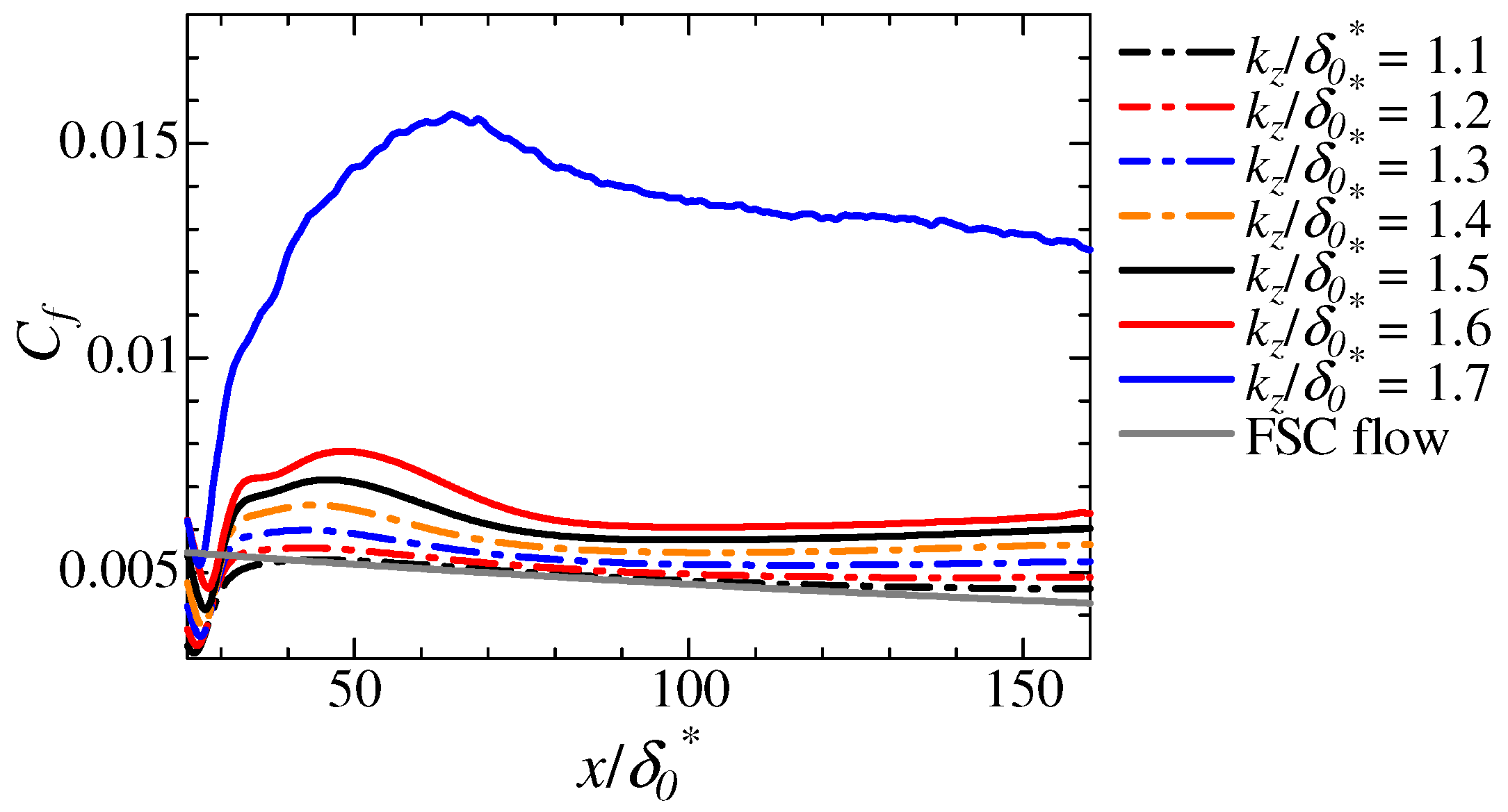
3.1. Roughness Height Dependency without Freestream Turbulence

First, we show the roughness height dependence of the transition processes for $Tu=0$, i.e., no FST condition. Since Brynjell-Rakola et al. [10] have reported an immediate transition at $k_z/{\delta }_0^{*}=1.7$ under the same condition, we here select $k_z/{\delta }_0^{*}=1.1$–$1.7$ ($R{e}_{kk}=342$–717) to investigate the transition processes via the crossflow instability.

Figure 3 shows the friction coefficient, $C_f$, where the wall shear stress involved in the definition of $C_f$ is the composite component of the chordwise and spanwise shear rates. The chordwise distribution of $C_f$ is suitable for discriminating transition processes. The trailing edge of the roughness cylinder is at $x/{\delta }_0^{*}=23.58$ and the figure plots the distribution from 25 to just before the fringe region. Also shown is the laminar solution of the FSC flow. For the lowest $k_z/{\delta }_0^{*}=1.1$, the profile follows the laminar solution well after a transient value immediately after roughness (indicating the presence of a cylinder wake). The deviation from the laminar profile seen around $x/{\delta }_0^{*}=150$ corresponds to the onset of CFV. As $k_z$ increases, the deviation moves upstream, and $C_f$ increases gradually in the entire flow field, but maintains low values for $k_z/{\delta }_0^{*}\le 1.6$. At $k_z/{\delta }_0^{*}=1.7$ ($R{e}_{kk}=717$), $C_f$ increases immediately after the roughness and reached a high value at $x/{\delta }_0^{*}\approx 60$. This is because the flow state becomes turbulent immediately behind the roughness, and such a transition process is referred to as the immediate transition. The threshold of the roughness Reynolds number under the condition of $Tu=0\%$ is found to be $666<R{e}_{kk,c}\le 717$, which is in good agreement with Ref. [10]. Figure 4 and Figure 5 show the two different transition processes of the gradual and immediate transitions observed at $k_z/{\delta }_0^{*}=1.3$ and $1.7$, respectively, where the vortical structures are visualized by Q-criterion [39].

For $k_z/{\delta }_0^{*}=1.3$, the long domain (cf. Table 1) is employed to observe the overall picture of the gradual transition. As seen in Figure 4, the vortex from the wake of the cylindrical roughness forms a CFV and it became turbulent at $x/{\delta }_0^{*}\approx 300$. Before being turbulent, secondary vortices occur on one side of the CFV: see Figure 4b for a close-up around $x/{\delta }_0^{*}\approx 220$. The secondary vortex is known as the finger vortex and is caused by the high-frequency secondary instability. The finger vortex covers the side to the top of the CFV, which type is the mode-z (type-$\mathrm{I}$) and mode-y (type-$\mathrm{I}\mathrm{I}$) secondary instability [10,15,40]. The finger vortex emerges primarily as the mode-z secondary instability and, as it moves downstream, the vortex reaches to the top of CFV and appears as the mode-y secondary instability. This mechanism is also reported by Casacuberta et al. [41]. The streamwise wavelength of the finger vortex is $\lambda /{\delta }_0^{*}\approx 14$, which is comparable to previously reported $\lambda /{\delta }_0^{*}\approx 13$ [10] and ≈16 [41], although the latter reference named the finger vortex a ridge-like structure. Note here that streamwise refers to the direction along the CFV. The finger vortex is a peculiar phenomenon to the CFV-dominated flow field, and no observation has been reported in the 2D boundary layer. In the FSC flow without FST, all gradual-transition processes follow the same path: (1) formation and growth of CFV, (2) generation of a finger vortex via high-frequency secondary instability, and (3) turbulent transition. Although not discussed in this study, a smooth surface without roughness exhibits a similar transition process but with traveling CFV [6,22].

The immediate transition process shown in Figure 5 is accompanied by hairpin vortices generated along a low-speed streak behind the roughness. The hairpin-vortex generation due to a high roughness was reported for a swept wing [25] and a Blasius boundary layer [42]. Its streamwise wavelength is $\lambda /{\delta }_0^{*}\approx 10$, which is consistent with a DNS result ($\lambda /{\delta }_0^{*}\approx 8$) for an infinite swept wing [25], but significantly different from the 2D boundary layer value ($\lambda /{\delta }_0^{*}\approx 4.7$) [42]. The wavelength of the hairpin vortex is extended by a factor of about two in the FSC boundary layer. The hairpin vortex enhances mixing between the near-wall low-momentum fluid and the freestream high-momentum fluid, resulting in turbulent production. Consequently, the flow fields become turbulent effectively in the wake of the roughness, that is, the immediate transition process absent of CFV. These results including the wavelengths of the hairpin and finger vortices may suggest a physical model and guidelines such as the required spatial resolution for LES [26] to resolve the secondary instabilities and to tract the transition process in the three-dimensional boundary layer.

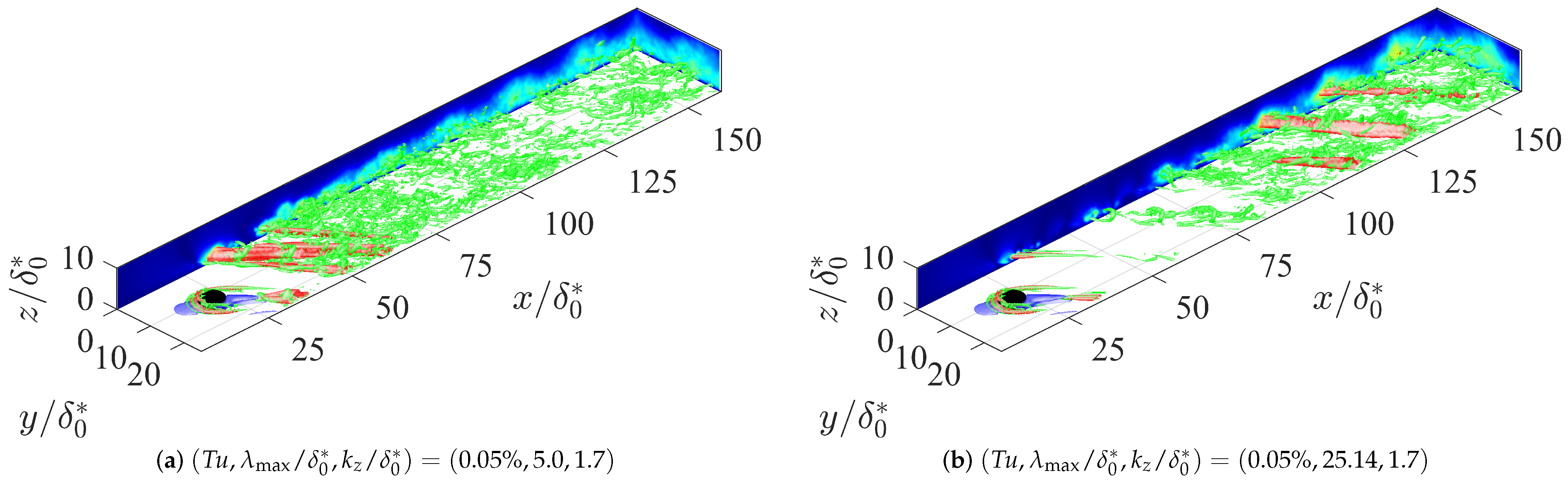
3.2. Different Transition Process

Freestream turbulence represents disturbances in the mean flow of an aircraft flight environment or wind tunnel experiment. When subjected to FST, the CFV in the flow field should be affected by the intensity of FST [23], resulting in the chordwise shift of the turbulent transition point [24,25]. The critical roughness Reynolds number for the immediate transition is $R{e}_{kk,c}=666$–717 when $Tu=0$, as reported in Section 3.1, but this will change under the influence of FST with $Tu\ne 0$. In the following, we discuss not only the intensity of the FST, but also the effect of their peak wavelengths.

Figure 6 is the main result, which shows the dependence of $R{e}_{kk,c}$ on the FST intensity ($Tu$) and the peak wavelength of the FST (${\lambda }_{\max }$). Here, $R{e}_{kk,c}=717$ is determined as the threshold under the no-FST condition, as described in the previous subsections. Similar values were obtained under the short-${\lambda }_{\max }$ and low-$Tu$ condition and under the long-${\lambda }_{\max }$ and high-$Tu$ condition, which correspond to the leftmost and rightmost plots in the figure, respectively. Compared to this, $R{e}_{kk,c}$ for the short-${\lambda }_{\max }$ remainss constant or slightly decreases as $Tu$ increases: that is, the immediate transition is promoted. In contrast, $R{e}_{kk,c}$ increases under the long-${\lambda }_{\max }$ condition for $Tu<0.1\%$: that is, the immediate transition is suppressed. The peak wavelength of FST clearly affects the turbulent transition, and there are mechanisms that promote or suppress the immediate transitions.

Let us address two parameter sets of $(Tu,{\lambda }_{\max })=(0.05\%,25.14)$ and $(0.05\%,5.0)$ as the cases where $R{e}_{kk,c}$ increases and decreases, respectively, and discuss the variations in the flow fields depending on the roughness height. The friction coefficients for various $k_z$ are shown in Figure 7. Under all the conditions with roughness height $k_z/{\delta }_0^{*}=1.1$–$1.7$, the turbulent transition occurs earlier (i.e., more upstream) in the case of short-${\lambda }_{\max }$ FST. In particular, even for the lowest $k_z/{\delta }_0^{*}=1.1$, the transition position can be confirmed at $x/{\delta }_0^{*}\approx 150$, where $C_f$ attains the turbulent value of about 0.014: see (b). Note here that, without FST, the transition does not occur within this domain for $k_z/{\delta }_0^{*}\le 1.6$. As for the long-${\lambda }_{\max }$ condition, the $C_f$ profiles are similar to those without FST for $k_z/{\delta }_0^{*}\le 1.3$: compare Figure 3 and Figure 7a. A significant deviation from the FSC laminar profile can be identified even at a still-low $k_z/{\delta }_0^{*}=1.4$. As $k_z$ increases, the transition point emerges in $x/{\delta }_0^{*}<150$ and shifts upstream. However, it should be noted that the $C_f$ profile jumping from the laminar to turbulent values is different from that of the immediate transition. The latter profile is steep and slightly convex upward, as in the case of $k_z/{\delta }_0^{*}\ge 2.0$ in Figure 7a. In contrast, for $k_z/{\delta }_0^{*}=1.4$–$1.9$, the profile is gently increasing and convex downward. It may be characterized by a plateau after the deviation from the laminar profile. Such a transition in the $C_f$ distribution is similar to that seen in the natural transition process via CFV, which is seen more downstream than $150{\delta }_0^{*}$ without FST [17]. We interpret these transition processes, observed in Figure 7a, as an ‘early transition’ of CFV due to FST. The mechanisms causing the early transition will be discussed in Section 3.3. As for the threshold of the immediate transition, Figure 7b reveals $R{e}_{kk,c}=666$ ($k_z/{\delta }_0^{*}=1.6$) under the short-${\lambda }_{\max }$ FST condition, implying that the immediate transition process occurs at a low roughness height due to the FST. Even in the case of $k_z/{\delta }_0^{*}\le 1.6$, the turbulent transition occurs much earlier than under the no-FST condition ($k_z/{\delta }_0^{*}<1.7$). This early transition of CFV due to FST is in agreement with Refs. [24,25]; in other words, they discussed the effects of FST at relatively short wavelengths. Our result also demonstrates that the long-${\lambda }_{\max }$ FST results in a downstream shift of the transition position ($x/{\delta }_0^{*}\approx 110$) for $R{e}_{kk}=717$ ($k_z/{\delta }_0^{*}=1.7$), whereas it is located more upstream at $x/{\delta }_0^{*}\approx 60$ under the no-FST and short-${\lambda }_{\max }$ conditions because of the immediate transition for the long-${\lambda }_{\max }$ FST with $Tu=0.05\%$, $R{e}_{kk,c}=967$. This is the highest $R{e}_{kk,c}$ obtained in our study (with $d/k\approx 3.2$) and is larger than, though not far off, those reported previously [16,25,43]: for a plot of $\sqrt{R{e}_{kk,c}}$ versus $d/k$, see Ref. [16]. The benchmark for $R{e}_{kk,c}$ was reported by von Doenhoff and Braslow [43] and other references [16,25], including various data in the literature. The present minimum $R{e}_{kk,c}=666$ (for $d/k\approx 3.8$) is also on the upper side of the scattered existing data set. This slight deviation is due to differences in how to determine the critical values in the DNS and experiments, as well as the measurement environment including FST. The experimentally obtained $R{e}_{kk,c}$ are shifted slightly downward compared to DNS because the numerical study can measure the $C_f$ distribution more rigorously. A recent experiment [20] reported $R{e}_{kk,c}\approx 200$ with another criterion based on the detection of turbulent transition fronts at a defined location of $x/c\approx 0.07$ ($98{\delta }_0^{*}$ downstream from the cylinder), using a two-dimensional determination based on the difference in heat transfer between laminar and turbulent flows. If the same criterion is employed here, our obtained critical values are revised lower: that is, $R{e}_{kk,c}<342$ and $538<R{e}_{kk,c}<583$ for short- and long-${\lambda }_{\max }$ FST conditions, respectively. The much lower value of $R{e}_{kk,c}\approx 200$ by Zoppini et al. [20] may be due to an early transition caused by short wavelength components of FST. The difference from an early experiment [43] also suggests some dependencies on the FST intensity and wavelength. The following section discusses the FST dependences of both the early transition and the immediate transition.

3.3. Transition Mechanisms with Freestream Turbulence

The parametric study in terms of the roughness height and FST wavelength is reported here with fixing $Tu=0.05\%$, at which the dependency on ${\lambda }_{\max }$ is pronounced as seen in Figure 6.

Figure 8 shows the dependence of the $C_f$ distribution on ${\lambda }_{\max }$ at the lowest $k_z/{\delta }_0^{*}=1.1$. Transition does not occur within the short domain for the long ${\lambda }_{\max }/{\delta }_0^{*}\ge 12.57$. For the short ${\lambda }_{\max }/{\delta }_0^{*}<12.57$, a gradual increase in $C_f$ and its asymptote to the turbulent value can be identified as features of the early transition. In particular, for ${\lambda }_{\max }/{\delta }_0^{*}\le 5.0$, the process of the early transition is completed within the domain.

We discuss the mechanism of the early transition under the condition of ${\lambda }_{\max }/{\delta }_0^{*}=5.0$. Figure 9a shows the flow field for $k_z/{\delta }_0^{*}=1.1$, where $C_f$ deviates from the laminar profile at $x/{\delta }_0^{*}\approx 50$ and grows almost linearly, as seen in Figure 7b. Consistent with this $C_f$ profile, hairpin vortices are generated at $x/{\delta }_0^{*}\approx 50$ and propagated downstream along the low-speed streak with inducing many vortices. Note that the low-speed streak originated from the roughness. One may find a new small hairpin vortex on the streak, as depicted in Figure 5c, at $x/{\delta }_0^{*}=50$ in Figure 9a. The hairpin and low-speed structures are common at higher roughness, but the onset of hairpin vortices move upstream, as observed in Figure 9b. Such a hairpin vortex was also detected in the swept-wing case by Vincentiis et al. [25], even in a high $Tu$ and low $k_z$ condition. They reported that temporal disturbances induced hairpin vortices in the roughness wake and were dependent on the FST intensity and wavelength. Given long-${\lambda }_{\max }$ FST, the hairpin vortex nor turbulent transitions are no longer recognized, as visualized in Figure 9c. Although the parameters other than ${\lambda }_{\max }$ are the same as in (b), the transition point has moved downstream outside the short domain. Using the long domain, we recognized the finger vortex (figure not shown), which is the same structure reported in previous studies [10,15] as a step of the secondary instability of CFV, at $x/{\delta }_0^{*}\approx 160$. Note again that the finger vortex occurs on a side of a well-developed CFV, whereas the hairpin vortex occurs on an undeveloped CFV due to the presence of disturbance either from FST or roughness element. A slight increase in $k_z$ from the condition in (c) has actually produced the hairpin vortex: find three well-shaped hairpin vortices at $x/{\delta }_0^{*}=60$–75 in Figure 9d. In this case, the hairpin vortex is caused by the combination of disturbances that are emanating from the high-roughness edge and long-${\lambda }_{\max }$ FST. The complex combination determines the type of the secondary-vortex (-instability) structure. The strong magnitude of disturbance emanating from a high-roughness edge triggers the onset of the hairpin vortex, resulting in the early transition. As for the FST, its short wavelengths promote the hairpin vortex via high-frequency secondary instability. In contrast, the long-wavelength condition suppressed hairpin vortices, but early hairpin vortex formation was again observed as the roughness height increased. We may conclude that the upstream shift of the transition position is due to the FST short wavelength and high roughness height, both of which enhance the secondary instability in the form of the hairpin vortex. Some numerical and experimental studies [12,23] showed FST-enhanced secondary instabilities, although they focused only on the FST intensity. In addition to this, the present results found the enhancement in the secondary instability depends on the FST wavelength in addition to its intensity.

Figure 10 shows two types of the secondary instability and their onsets around the near-wall low-speed region. The panels in the left column are for the hairpin vortex associated with the early transition, two legs of which can be clearly seen at $(y/{\delta }_0^{*},z/{\delta }_0^{*})\approx (4,1)$ and $\approx (7,3)$ in (a). As shown in (c), the hairpin vortex induces a blowing up of low-speed fluid and a blowing down of high-speed fluid, which are ejection and sweep events, respectively. These events are similar to those by typical coherent structures observed in the near-wall turbulence [44]. The disturbances due to the hairpin vortex spread in the spanwise direction as well as the low-speed streak direction, as shown in Figure 9b. The way the disturbance spreads throughout the low-speed streak is different to that of the finger vortex, described later, but rather similar to that of a zero-pressure-gradient boundary layer [45]. The spanwise-averaged ${\overline{w}}_{\mathrm{RMS}}$ distribution, plotted in (e), reveals a much higher ${\overline{w}}_{\mathrm{RMS}}$ at the height of the hairpin vortex ($z/{\delta }_0^{*}\approx 1$–3) than without FST. Such a high $w_{\mathrm{RMS}}$ value is a cause of the early transition process. Although the turbulent transition on the swept flat plate is generally caused by the finger vortex as the secondary instability [12,13], the short-${\lambda }_{\max }$ FST-induced hairpin vortex should be also of interest. The hairpin and finger vortices share the role of collapsing the stationary vortex. The disturbance caused by the hairpin vortex plays the role of a high-frequency secondary instability, which is a direct cause of the transition to turbulence.

As for the finger vortex observed under the long-${\lambda }_{\max }$ FST condition, we can identify its leg at $(y/{\delta }_0^{*},z/{\delta }_0^{*})\approx (23,1)$ in Figure 10b. Note here the spanwise periodicity of the domain. The positions of the finger vortex and its high $w_{\mathrm{RMS}}$ region, as in (d), are at a side of low-speed region. This feature is in common with the secondary instability in the no-FST condition. Here, the contour of $w_{\mathrm{rms}}/U_0$ in the no-FST condition is plotted in Figure 11, for reference. A strong temporal disturbance due to the finger vortex can be detected at $(y/{\delta }_0^{*},z/{\delta }_0^{*})\approx (17,3)$, which corresponds to a side of CFV. The three-dimensional visualization in Figure 4 also reveals the finger vortex extending from the side to the top of CFV. This vortex position corresponds to the location of the high-frequency secondary instability [13]. This type of high-frequency secondary instability that occurs at the side of CFV is classified as the z-mode (type-I) secondary instability [13,15,40]. However, a slightly different aspect is found in the ${\overline{w}}_{\mathrm{RMS}}$ profile, which is plotted in Figure 10f and shows a peak at higher $z/{\delta }_0^{*}\approx 4$ than the hairpin vortex position. This position is the top of the CFV, so it is defined as the y-mode (type-$\mathrm{I}\mathrm{I}$) of the high-frequency secondary instability [13,15,40]. The weaker disturbances are also distributed at the side of CFV, as in Figure 10d, indicating coexistence of the z-mode. The position of the finger vortex was also shifted upstream significantly compared to the no-FST condition. Under long-${\lambda }_{\max }$ FST conditions, as reported by Högberg and Henningson [12] and Downs and White [23], FST shifts not only the transition position, but also the secondary instability upstream (compared to the no-FST condition).

We have shown that the FST wavelength alters a secondary vortex structure that triggers a turbulent transition, by visualizing the instantaneous flow field and the disturbance distribution. The short-${\lambda }_{\max }$ FST corresponds to a higher-frequency fluctuation that approaches the boundary layer. To investigate the effect of inflowing FST, we performed a frequency analysis of the temporal disturbance, for roughness height $k_z/\delta =1.3$. The measurement time period is $T^{*}\approx 391$ ($T^{*}=T{U}_0/{\delta }_0^{*}$), and the sampling rate is $\mathsf{\Delta }{t}^{*}\approx 0.0977$. The result is shown in Figure 12. A peak at $\omega \approx 0.08$ appears regardless of ${\lambda }_{\max }$. This peak is attributed to the limited length of the disturbance box $(L_{dx}/{\delta }_0^{*}=80)$, and the disturbance box repeatedly inflows into the flow field. The inflow rate of the disturbance box was $T^{*}=80$, which was $\omega (=2\pi /T^{*})\approx 0.0785$. The wavelength ${\lambda }_{\max }/{\delta }_0^{*}=25.14$ is equivalent to the low-frequency disturbance of $\omega \approx 0.25$, and ${\lambda }_{\max }/{\delta }_0^{*}=5.0$ is the high-frequency disturbance $\omega \approx 1.26$. In particular, the high frequency is comparable to the high-frequency range tested by Högberg and Henningson [12]. The high-frequency range of $\omega >{10}^0$ is unstable on the CFV [10,30]. The high-frequency secondary instability that occurs during the development of the CFV is induced near the cylindrical roughness by the short-${\lambda }_{\max }$ FST. It is the mechanism of the early transition process by the hairpin vortex.

3.4. Disturbance from High Roughness Upper Edge

The previous section has demonstrated that, under the non-immediate transition condition, the presence of FST accelerates the turbulent transition. However, under the long-${\lambda }_{\max }$ FST condition, the immediate transition is delayed and the threshold $R{e}_{kk,c}$ is increased (see Figure 6). In the following, we discuss the mechanism by which the long-${\lambda }_{\max }$ FST suppresses disturbances caused by the high roughness.

We show a 3D visualization of the flow field at $k_z/{\delta }_0^{*}=1.7$ in Figure 13, where the vortex distribution at an arbitrary instant and time-averaged disturbance intensity are visualized simultaneously. The high-$w_{\mathrm{RMS}}/U_0$ region, shown in red in the figure, corresponds to temporal fluctuations that may trigger a turbulent transition, such as the secondary instability and disturbance from the roughness edge. This suggests the beginning of the turbulent transition. Under the immediate transition condition (Figure 13a), the high $w_{\mathrm{RMS}}/U_0$ extends from the cylindrical roughness to the wake. The flow over the high cylindrical roughness already has high disturbances, which leads to the immediate transition. This high disturbance emanating from the roughness is suppressed under long-${\lambda }_{\max }$ conditions (Figure 13b). This results in the non-immediate transition process with a stationary vortex. The suppression mechanism is also true under the higher roughness condition ($k_z/{\delta }_0^{*}<2.0$).

In order to determine a frequency at which the disturbance due to high roughness is suppressed, we performed the frequency analysis for $k_z/{\delta }_0^{*}=1.7$, as shown in Figure 14. The method and sampling conditions are same with those for Figure 12. The measurement point is near the upper edge of the cylindrical roughness where the high-frequency disturbance occurs. Comparison with the no-FST condition shows a significant decrease in the high-frequency region of $\omega >{10}^0$ for the long-${\lambda }_{\max }$ FST. The nominal frequency of long ${\lambda }_{\max }/{\delta }_0^{*}=25.14$ is $\omega \approx 0.25$. As a result, the flow with suppressed immediate transitions undergoes turbulent transitions far downstream due to low-frequency disturbances, as shown in Figure 13b. Figure 15 shows the schematics of immediate transition suppression mechanisms. The wavelength of the FST affects the roughness height threshold ($R{e}_{kk,c}$) of the immediate transition, via the suppression of high-frequency disturbance from the high roughness edge.

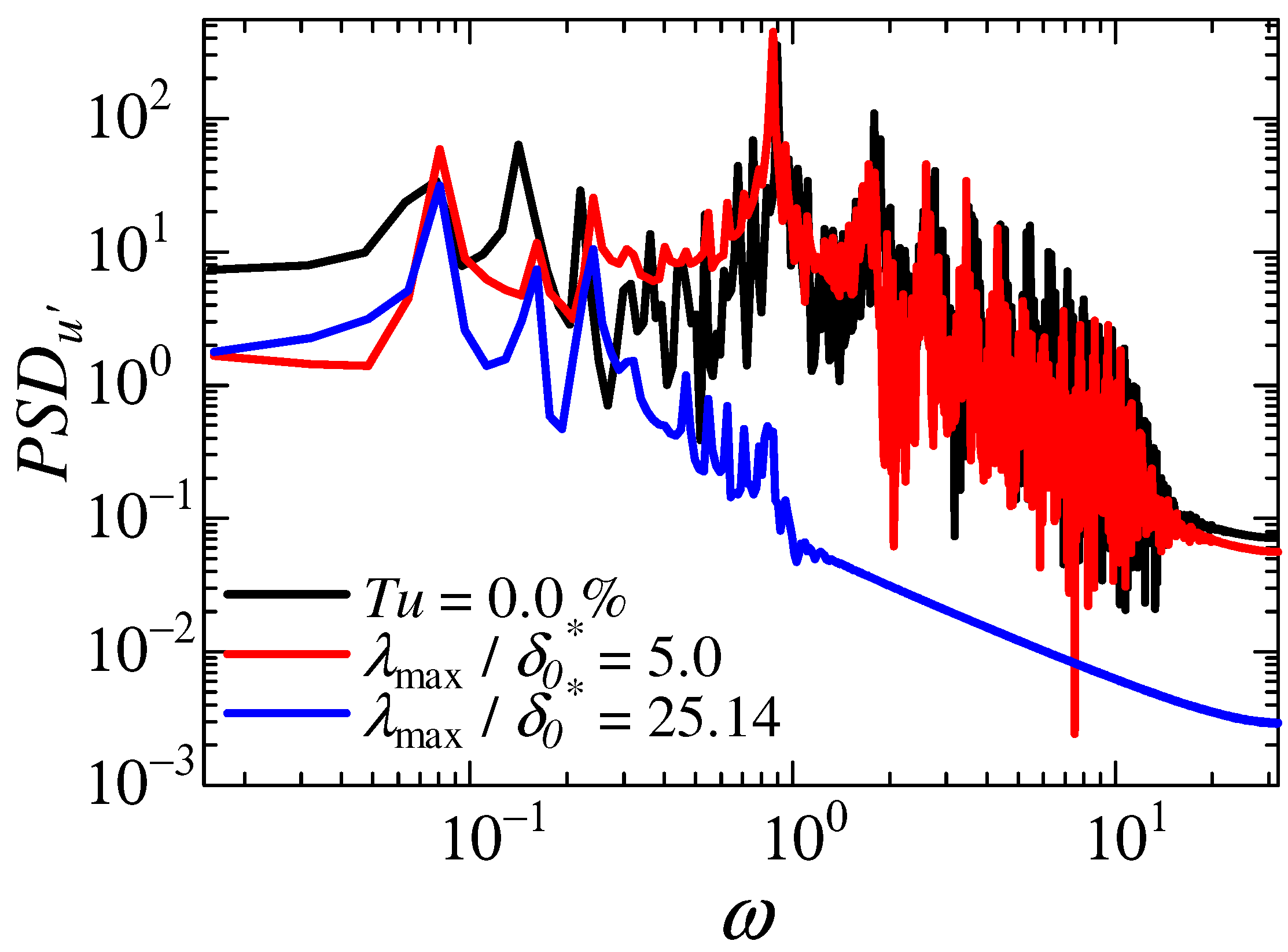
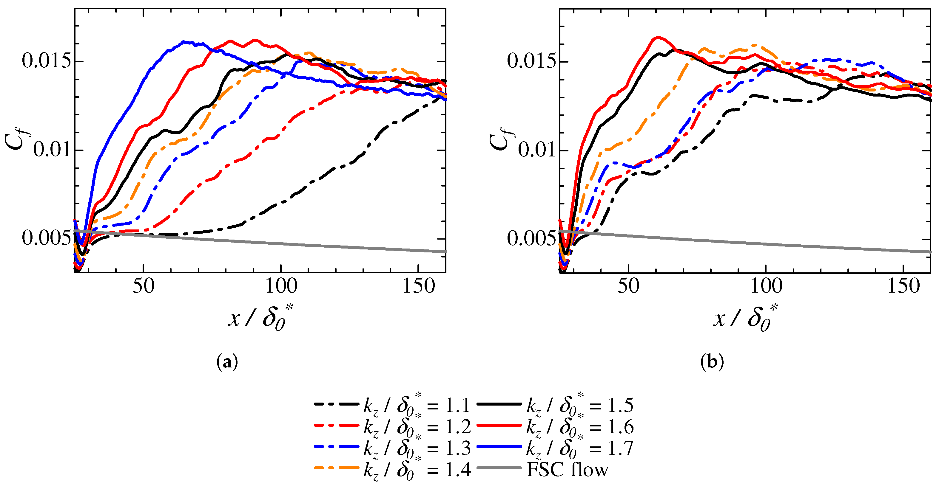
3.5. Turbulent Intensity Dependence on Transition Mechanisms

We have shown the peak-wavelength (${\lambda }_{\max }$) dependence of the turbulent transition process via the CFV. Next, we discuss the dependence on the FST intensity. The CFV and its secondary instability were known to be accelerated by high FST intensity [24,25]. The current study will confirm that, even under conditions controlled by the peak wavelength, a strong FST should cause an earlier transition.

Figure 16 shows the friction coefficient distribution for $Tu=0.5\%$. Compared to Figure 7 for $Tu=0.05\%$, the turbulent transition position is farther upstream, irrespective of the roughness height. The threshold for the immediate transition is also lower, as shown in Figure 6. The dependence on the FST intensity under the short-${\lambda }_{\max }$ condition was less than that under the long-${\lambda }_{\max }$ condition: compare Figure 16a,b. The difference in the turbulent transition position is insignificant. This is because, even under long ${\lambda }_{\max }$ conditions, as with short ${\lambda }_{\max }$, a strong FST intensity leads to an early transition with hairpin vortices. In the case of long-${\lambda }_{\max }$ FST, the difference in the turbulent intensity is more effective than under the short-${\lambda }_{\max }$ condition at the same roughness height. Figure 17 visualizes the hairpin vortices for the long-${\lambda }_{\max }$, high-$Tu$ FST. One can detect the hairpin vortex at $x/{\delta }_0^{*}\approx 40$. Note here that, as shown in Figure 9c, no hairpin vortex occurs under the same condition but with low-$Tu$. In other words, the condition of the hairpin vortex generation depends on the FST intensity. This vortex structure is the same as that observed for the short ${\lambda }_{\max }$ FST. The hairpin vortex must be a cause of the high-frequency secondary instability downstream. Figure 18 shows the frequency analysis for different FST intensities with fixed ${\lambda }_{\max }/{\delta }_0^{*}=25.14$. The measurement point is located slightly downstream of the onset of hairpin vortex, while this measurement point is behind the stationary vortex because of the absence of hairpin vortex in the case of low $Tu=0.05\%$: see Figure 9c. High-frequency disturbances ($\omega >{10}^0$) downstream of the hairpin vortex can be confirmed from the frequency analysis, under the high-$Tu$ condition. This means that the hairpin vortex triggers turbulent transition as the high-frequency secondary instability. The subsequent process of the early transition is identical to that seen in the case of high $k_z$ and short ${\lambda }_{\max }$. Figure 19 shows the wall-normal distribution of spanwise-averaged ${\overline{w}}_{\mathrm{RMS}}/U_0$, at the same chordwise position as in Figure 18. Under the long-${\lambda }_{\max }$ condition, the ${\overline{w}}_{\mathrm{RMS}}/U_0$ is low and independent of $Tu$, except for the case of $Tu=0.5\%$. The increase for $Tu=0.5\%$ is attributed to the onset of hairpin vortices. Its profile is consistent with those for the short-${\lambda }_{\max }$ FST, which generates hairpin vortices irrespectively of the FST intensity. The suppression of the early transition by the long wavelength contained in FST is limited to low-intensity ($Tu\le 0.1\%$). This is the same trend as the suppression of the immediate transition, i.e., the increase in $R{e}_{kk,c}$.

4. Conclusions

Using direct numerical simulations, we performed a parametric study on the turbulent transition process in the swept flat-plate boundary layer, in terms of the roughness height and the peak wavelength and intensity of the freestream turbulence (FST). The isolated cylindrical roughness was considered as a disturbance source that generates stationary crossflow vortices (CFV).

With high roughness, turbulent transitions are induced immediately after the roughness element without the formation of CFV. The critical roughness height, $R{e}_{kk,c}$, for the so-called immediate transition was investigated under various FST conditions and summarized in Figure 6. There occurs a slight decrease in $R{e}_{kk,c}$ due to the presence of FST, but notably, the weak long-wavelength FST ($Tu\le 0.1$ and ${\lambda }_{\max }/{\delta }_0^{*}\ge 12.57$) provides an increase in $R{e}_{kk,c}$, i.e., a delay of the immediate transition. Similarly, this delay effect by the weak long-wavelength FST is also observed in the early turbulent transition that occurs before the growing CFV saturates. The FST affects the high-frequency secondary instability in the process of the early turbulent transition. In particular, the short-wavelength FST induces high-frequency secondary instability on the stationary vortices, resulting in the early turbulent transitions before the saturation of growing CFV. In the early transition, hairpin vortices are generated instead of the finger vortex, which is a typical secondary vortex structure of the CFV. Although it is shown that FST induces hairpin vortices and promotes immediate transition in Ref. [25], we reveal a new scenario of hairpin-vortex induction by the high-frequency secondary instability. The hairpin vortex is similar to the finger vortex in terms of its inducing vortical flow and instability to lead high-frequency disturbance. The hairpin vortex plays a role to trigger the early transition farther upstream of the secondary instability of CFV with the finger vortex. The long-wavelength FST suppressed the hairpin vortex to induce high-frequency disturbance from the high cylindrical roughness. This is the mechanism leading to the suppression of the immediate transition. The interaction between the peak wavelength of the FST and stationary CFV was observed even under high-FST-intensity conditions. We conclude that the roughness height thresholds for hairpin vortex generation and immediate transition depend on the FST intensity and wavelength. The cylindrical roughness examined here is larger than roughness amplitudes on typical polished wing surfaces and should be dominant to the CFV induction, as experiments have confirmed its dominance [40]. The excitation by FST occurs especially on the wake vortex of the cylindrical roughness. Accordingly, the FST dependency reported here would be common even for the actual wing surface.

According to the present result, including Figure 6, one can predict the contribution of both the FST and roughness to turbulent transitions for their experiment. For example, Zoppini et al. [20] experimentally reported the early transitions at low-roughness Reynolds numbers. This can be reasonably explained by considering that the high-frequency component of FST had collapsed the wake vortex effectively, yielding the early transitions. However, this study focuses on the dependence on a single peak wavelength. In flight and wind tunnel tests, FST includes a wide range of wavelengths and the interactions between FST and CFV should be more complex. The complex interactions need to be clarified by analysis of harmonics with energy in a wide spectral band. In addition, it is necessary to investigate the lower threshold of roughness height that causes early transition due to high-frequency FST. Such a threshold would help to improve the prediction performance of the turbulent transition location depending on the conditions of in-flight aircraft or wind-tunnel model experiment. This is another reason why the spectral and spatial distribution of FST should be considered when modeling FST numerically, at least in cross-flow instability studies.

References

1. Denham, C.L.; Patil, M.; Roy, C.J.; Alexandrov, N. Framework for estimating performance and associated uncertainty for modified aircraft configurations. Aerospace 2022, 9, 490. [Google Scholar] [CrossRef]
2. Buntov, M.Y.; Makeev, P.V.; Ignatkin, Y.M.; Glazkov, V.S. Numerical modeling of the walls perforation influence on the accuracy of wind tunnel experiments using two-dimensional computational fluid dynamics model. Aerospace 2022, 9, 478. [Google Scholar] [CrossRef]
3. Jiménez-Portaz, M.; Chiapponi, L.; Clavero, M.; Losada, M.A. Air flow quality analysis of an open-circuit boundary layer wind tunnel and comparison with a closed-circuit wind tunnel. Phys. Fluids 2020, 32, 125120. [Google Scholar] [CrossRef]
4. Guissart, A.; Romblad, J.; Nemitz, T.; Tropea, C. Small-scale atmospheric turbulence and its impact on laminar-to-turbulent transition. AIAA J. 2021, 59, 3611–3621. [Google Scholar] [CrossRef]
5. Kohama, Y. Some expectation on the mechanism of cross-flow instability in a swept wing flow. Acta Mech. 1987, 66, 21–38. [Google Scholar] [CrossRef]
6. Saric, W.S.; Reed, H.L.; White, E.B. Stability and transition of three-dimensional boundary layers. Annu. Rev. Fluid Mech. 2003, 35, 413–440. [Google Scholar] [CrossRef] [Green Version]
7. Yakeno, A.; Obayashi, S. Propagation of stationary and traveling waves in a leading-edge boundary layer of a swept wing. Phys. Fluids 2021, 33, 094111. [Google Scholar] [CrossRef]
8. Lin, P.; Wu, J.; Lu, L.; Xiong, N.; Liu, D.; Su, J.; Liu, G.; Tao, Y.; Wu, J.; Liu, X. Investigation on the Reynolds number effect of a flying wing model with large sweep angle and small aspect ratio. Aerospace 2022, 9, 523. [Google Scholar] [CrossRef]
9. Chen, X.; Xi, Y.; Ren, J.; Fu, S. Cross-flow vortices and their secondary instabilities in hypersonic and high-enthalpy boundary layers. J. Fluid Mech. 2022, 947, A25. [Google Scholar] [CrossRef]
10. Brynjell-Rahkola, M.; Shahriari, N.; Schlatter, P.; Hanifi, A.; Henningson, D.S. Stability and sensitivity of a cross-flow-dominated Falkner-Skan-Cooke boundary layer with discrete surface roughness. J. Fluid Mech. 2017, 144, 830–850. [Google Scholar] [CrossRef] [Green Version]
11. Loiseau, J.C.; Robinet, J.C.; Cherubini, S.; Leriche, E. Investigation of the roughness-induced transition: Global stability analyses and direct numerical simulations. J. Fluid Mech. 2014, 760, 175–211. [Google Scholar] [CrossRef] [Green Version]
12. Högberg, M.; Hennigson, D. Secondary instability of a cross-flow vortices in Falkner-Skan-Cooke boundary layer. J. Fluid Mech. 1998, 368, 339–357. [Google Scholar] [CrossRef]
13. Malik, M.R.; Li, F.; Choudhari, M.M.; Chang, C.L. Secondary instability of a cross-flow vortices and swept-wing boundary-layer transition. J. Fluid Mech. 1999, 399, 85–115. [Google Scholar] [CrossRef]
14. Bonfigli, G.; Kloker, M. Secondary instability of crossflow vortices: Validation of the stability theory by direct numerical simulation. J. Fluid Mech. 2007, 583, 229–272. [Google Scholar] [CrossRef] [Green Version]
15. Wassermann, P.; Kloker, M. Mechanisms and passive control of crossflow-vortex-induced transition in a three-dimensional boundary layer. J. Fluid Mech. 2002, 456, 49–84. [Google Scholar] [CrossRef] [Green Version]
16. Kurz, B.E.H.; Kloker, J.M. Mechanisms of flow tripping by discrete roughness elements in a swept-wing boundary layer. J. Fluid Mech. 2016, 796, 158–194. [Google Scholar] [CrossRef]
17. Ishida, T.; Tsukahara, T.; Tokugawa, N. Parameter effects of spanwise-arrayed cylindrical roughness elements on transition in the Falkner–Skan–Cooke boundary layer. Trans. Jpn. Soc. Aeronaut. Space Sci. 2022, 65, 84–94. [Google Scholar] [CrossRef]
18. Ishida, T.; Ohira, K.; Hosoi, R.; Tokugawa, N.; Tsukahara, T. Numerical and experimental analysis of three-dimensional boundary-layer transition induced by isolated cylindrical roughness elements. Int. J. Aeronaut. Space Sci. 2022, 23, 649–659. [Google Scholar] [CrossRef]
19. Örlü, R.; Tillmark, N.; Alfredsson, P.H. Measured Critical Size of Roughness Elements; Technical Report by KTH Royal Institude of Technology: Stockholm, Sweden, 2021. [Google Scholar]
20. Zoppini, G.; Westerbeek, S.; Ragni, D.; Kotsonis, M. Receptivity of crossflow instability to discrete roughness amplitude and location. J. Fluid Mech. 2022, 939, A33. [Google Scholar] [CrossRef]
21. Saric, W.S.; Reed, H.L.; Kerschen, E.J. Boundary-layer receptivity to freestream disturbance. Annu. Rev. Fluid Mech. 2002, 34, 291–319. [Google Scholar] [CrossRef] [Green Version]
22. Deyhle, H.; Bippes, H. Disturbance growth in an unstable three-dimensional boundary layer and its dependence on environmental conditions. J. Fluid Mech. 1996, 316, 73–113. [Google Scholar] [CrossRef]
23. Downs, R.S.; White, E.B. Free-stream turbulence and the development of cross-flow disturbances. J. Fluid Mech. 2013, 735, 347–380. [Google Scholar] [CrossRef]
24. Hosseini, S.M.; Hanifi, A.; Hennigson, D.S. Effect of freestream turbulence on roughness-induced crossflow instability. Procedia IUTAM 2015, 14, 303–310. [Google Scholar] [CrossRef] [Green Version]
25. Vincentiis, L.D.; Henningson, D.S.; Hanifi, A. Transition in an infinite swept-wing boundary layer subject to surface roughness and free-stream turbulence. J. Fluid Mech. 2022, 931, A24. [Google Scholar] [CrossRef]
26. Huai, X.; Joslin, R.D.; Piomellt, U. Large-eddy simulation of boundary-layer transition on a swept wedge. J. Fluid Mech. 1999, 381, 357–380. [Google Scholar] [CrossRef]
27. Bose, S.T.; Park, G.I. Wall-modeled large-eddy simulation for complex turbulent flows. Annu. Rev. Fluid Mech. 2018, 50, 535–561. [Google Scholar] [CrossRef]
28. Chen, J.; Dong, S.; Chen, X.; Yuan, X.; Xu, G. Stationary cross-flow breakdown in a high-speed swept-wing boundary layer. Phys. Fluids 2021, 33, 024108. [Google Scholar] [CrossRef]
29. De Vanna, F.; Baldan, G.; Picano, F.; Benini, E. Effect of convective schemes in wall-resolved and wall-modeled LES of compressible wall turbulence. Comput. Fluids 2023, 250, 105710. [Google Scholar] [CrossRef]
30. Brynjell-Rahkola, M.; Schlatter, P.; Hanifi, A.; Henningson, D.S. Global stability analysis of a roughness wake in a Falkner-Skan-Cooke boundary layer. Procedia IUTAM 2015, 14, 192–200. [Google Scholar] [CrossRef] [Green Version]
31. Hosseini, S.M.; Tempelmann, D.; Hanifi, A.; Henningson, D.S. Stabilization of a swept-wing boundary layer by distributed roughness elements. J. Fluid Mech. 2013, 718, R1. [Google Scholar] [CrossRef]
32. Owen, M.; Frendi, A. Towards the understanding of humpback whale tubercles: Linear stability analysis of a wavy flat plate. Fluids 2020, 5, 212. [Google Scholar] [CrossRef]
33. Saric, W.S.; Carpenter, A.L.; Reed, H.L. Passive control of transition in three-dimensional boundary layers, with emphasis on discrete roughness elements. Philos. Transitions R. Soc. A 2011, 369, 1352–1364. [Google Scholar] [CrossRef]
34. Cooke, J.C. The boundary layer of a class of infinite yawed cylinders. In Mathematical Proceedings of the Cambridge Philosophical Society; Cambridge University Press: Cambridge, UK, 1950; Volume 46, pp. 645–648. [Google Scholar] [CrossRef]
35. Fadlun, E.; Verzicco, R.; Orlandi, P.; Mohd-Yusof, J. Combined immersed-boundary finite-difference methods for three-dimensional complex flow simulations. J. Comput. Phys. 2000, 161, 35–60. [Google Scholar] [CrossRef]
36. Muths, S.; Bhushan, S. Comparison between temporal and spatial direct numerical simulations for bypass transition flows. J. Turbul. 2020, 21, 311–354. [Google Scholar] [CrossRef]
37. Watanabe, D.; Maekawa, H. Rapid growth of unsteady finite-amplitude perturbations in a supersonic boundary-layer flow. In Ninth International Symposium on Turbulence and Shear Flow Phenomena; Begel House Inc.: Melbourne, Australia, 2015; Volume 3B-4. [Google Scholar] [CrossRef]
38. Brandt, L.; Schlatter, P.; Henningson, D.S. Transition in boundary layers subject to free-stream turbulence. J. Fluid Mech. 2004, 517, 167–198. [Google Scholar] [CrossRef] [Green Version]
39. Jeong, J.; Hussain, F. On the identification of a vortex. J. Fluid Mech. 1995, 285, 69–94. [Google Scholar] [CrossRef]
40. Serpieri, J.; Kotsonis, M. Three-dimensional organisation of primary and secondary crossflow instability. J. Fluid Mech. 2016, 799, 200–245. [Google Scholar] [CrossRef] [Green Version]
41. Casacuberta, J.; Groot, K.J.; Hickel, S.; Kotsonis, M. Secondary instabilities in swept-wing boundary layers: Direct Numerical Simulations and BiGlobal stability analysis. In AIAA SCITECH 2022 Forum; AIAA: San Diego, CA, USA, 2022; p. 2330. [Google Scholar] [CrossRef]
42. Bucci, M.A.; Puckert, D.K.; Andriano, C.; Loiseau, J.C.; Cherubini, S.; Robinet, J.C.; Rist, U. Roughness-induced transition by quasi-resonance of a varicose global mode. J. Fluid Mech. 2018, 836, 167–191. [Google Scholar] [CrossRef] [Green Version]
43. Von Doenhoff, A.E.; Braslow, A.L. The effect of distributed surface roughness on laminar flow. In Boundary Layer and Flow Control; Lachmann, G., Ed.; Pergamon: Amsterdam, The Netherlands, 1961; pp. 657–681. [Google Scholar] [CrossRef]
44. Robinson, S.K. Coherent motions in the turbulent boundary layer. Annu. Rev. Fluid Mech. 1991, 23, 601–639. [Google Scholar] [CrossRef]
45. Vaid, A.; Vadlamani, N.R.; Malathi, A.S.; Gupta, V. Dynamics of bypass transition behind roughness element subjected to pulses of free-stream turbulence. Phys. Fluids 2022, 34, 114110. [Google Scholar] [CrossRef]
Figure 1. Schematic of swept flat-plate boundary layer.
Aerospace 10 00128 g001
Figure 2. (a) Isosurfaces of chordwise disturbance velocity in the case of λ max / δ 0 * = 6.285 : red/blue shows positive/negative value. (b) Same as (a), but for λ max / δ 0 * = 25.14 . (c) Energy spectrum of velocity fluctuation in the disturbance box to be applied as FST for the main DNS on the FSC boundary layer. (d) FSC boundary layer profile at inlet to be used as a damping function for the superimposed disturbance.
Aerospace 10 00128 g002
Figure 3. Friction coefficient distribution for T u = 0 and different roughness heights.
Aerospace 10 00128 g003
Figure 4. Instantaneous flow field of k z / δ 0 * = 1.3 for T u = 0 . (a) Isosurface of chordwise velocity and vortical structure are visualized by u / U 0 = 0.3 (blue) and Q = 0.002 . The vortical structures are colored by u / U 0 from 0.0 (blue) to 1.5 (red). The color contour range in the x-y plane is the same as that of the colored isosurface. (b) Enlarged view. (c) Schematic of the finger vortex on the crossflow vortex.
Aerospace 10 00128 g004
Figure 5. Instantaneous flow field of k z / δ 0 * = 1.7 for T u = 0 . (a,b) Isosurface and color contours are the same as those in Figure 4, but Q = 0.2 . (c) Schematic of the hairpin vortex on a low-speed streak.
Aerospace 10 00128 g005
Figure 6. Dependence of the immediate-transition threshold ( R e k k , c ) on FST wavelength and intensity.
Aerospace 10 00128 g006
Figure 7. Friction coefficient distribution for T u = 0.05 % , with λ max / δ 0 * = 25.14 (a) and 5.0 (b).
Aerospace 10 00128 g007
Figure 8. Friction coefficient distribution for T u = 0.05 % and k z / δ 0 * = 1.1 .
Aerospace 10 00128 g008
Figure 9. Instantaneous flow field for different λ max / δ 0 * and k z / δ 0 * with fixed T u . The red isosurface indicates Q = 0.2 , corresponding to vortices; and the blue is u / U 0 = 0.3 , extracting low-speed streaks. The color contours are the same as those in Figure 4.
Aerospace 10 00128 g009
Figure 10. Cross-section visualization of secondary instability and its relevant wall-normal velocity magnitude, for two different λ max with fixed T u and k z : left column of (a,c,e), ( T u , λ max / δ 0 * , k z / δ 0 * ) = ( 0.05 % , 5.0 , 1.3 ) ; right column of (b,d,f), ( T u , λ max / δ 0 * , k z / δ 0 * ) = ( 0.05 % , 25.14 , 1.3 ) . The visualized y-z planes are respectively at x / δ 0 * = 40 and 160, because of the different chordwise positions at which the secondary instability occurs. (a,b) The color contour shows the chordwise velocity with the in-plane fluctuating velocity vector ( v , w ). (c,d) Root-mean-square value of temporal fluctuations in the wall-normal velocity, w RMS . (e,f) Wall-normal distribution of the spanwise averaged w RMS .
Aerospace 10 00128 g010
Figure 11. y-z plane distribution of w RMS / U 0 for k z / δ 0 * = 1.3 , T u = 0.0 % at x / δ 0 * = 240 .
Aerospace 10 00128 g011
Figure 12. Frequency analysis of u / U 0 for k z / δ 0 * = 1.3 at the top of CFV: ( x , y , z ) ( 50 , 16 , 2 ) .
Aerospace 10 00128 g012
Figure 13. Instantaneous vortex structure and time-averaged velocity field for a high k z / δ 0 * = 1.7 . The isosurfaces were Q = 0.2 (green), u ¯ / U 0 = 0 (blue), and w RMS / U 0 = 0.12 (red).
Aerospace 10 00128 g013
Figure 14. Frequency analysis of u / U 0 for k z / δ 0 * = 1.7 at ( x , y , z ) / δ 0 * ( 30 , 26 , 2 ) .
Aerospace 10 00128 g014
Figure 15. Schematics of the immediate transition (a) and the suppression mechanism (b).
Aerospace 10 00128 g015
Figure 16. Friction coefficient distribution for T u = 0.5 % , with λ max / δ 0 * = 25.14 (a) and 5.0 (b).
Aerospace 10 00128 g016
Figure 17. Instantaneous flow field of ( T u , λ max / δ 0 * , k z / δ 0 * ) = ( 0.5 % , 25.14 , 1.3 ) . The isosurfaces and color contours are the same as in Figure 9: left, whole domain; right, enlarged view.
Aerospace 10 00128 g017
Figure 18. Frequency analysis of u / U 0 for k z / δ 0 * = 1.3 , λ max / δ 0 * = 25.14 at ( x , y , z ) / δ 0 * ( 50 , 14 , 1 ) .
Aerospace 10 00128 g018
Figure 19. Wall-normal distribution at x / δ 0 * = 50 of w ¯ RMS / U 0 for (a) λ max / δ 0 * = 25.14 , (b) λ max / δ 0 * = 5.0 of k z / δ 0 * = 1.3 .
Aerospace 10 00128 g019