
Hugoniot Relation for a Bow-Shaped Detonation Wave Generated in RP Laser Propulsion
 , ,
, ,
Abstract
:1. Introduction
2. Numerical Methods
2.1. Numerical Models
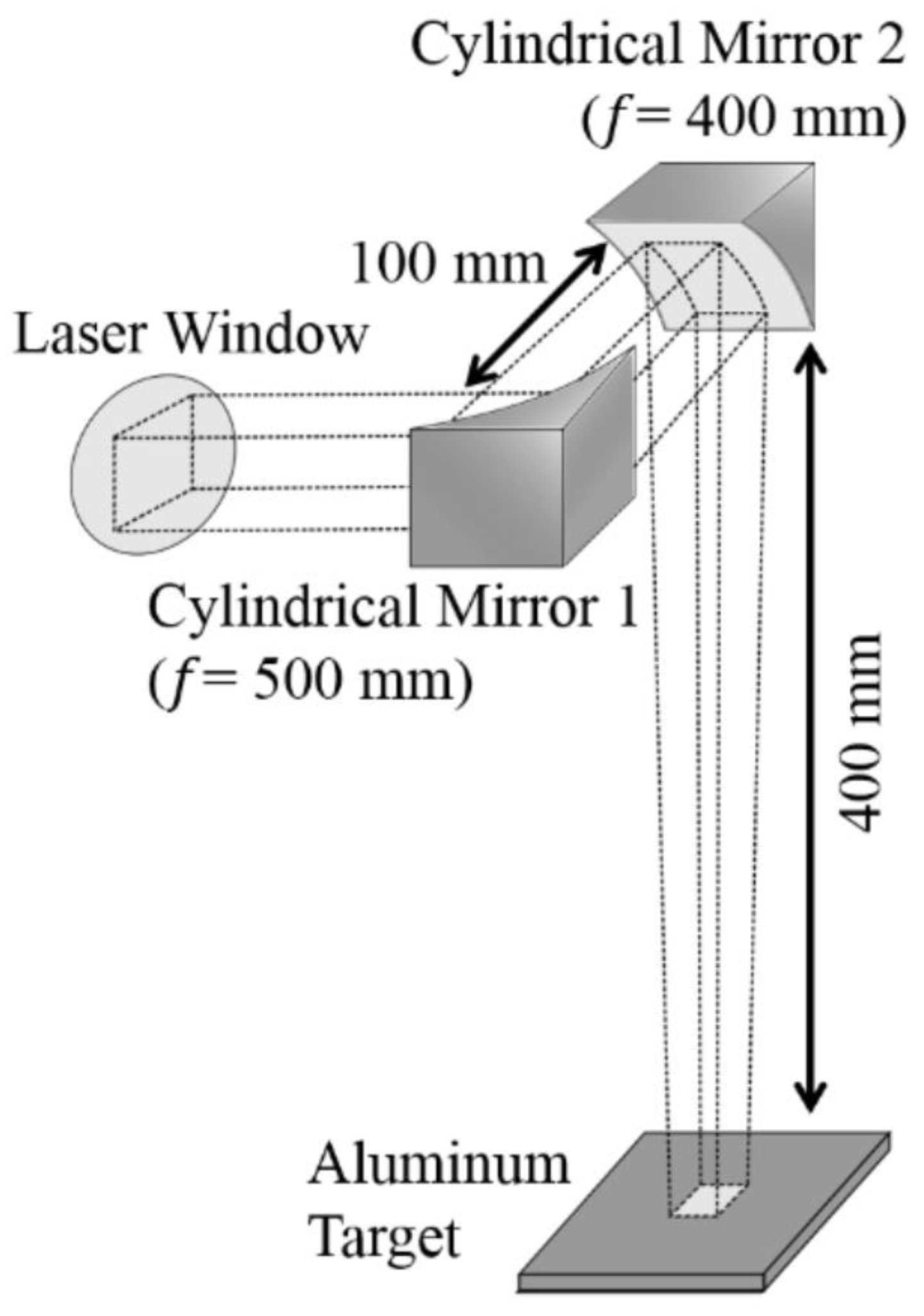
2.1.1. Analytical Model Reproducing the Experiment Conditions
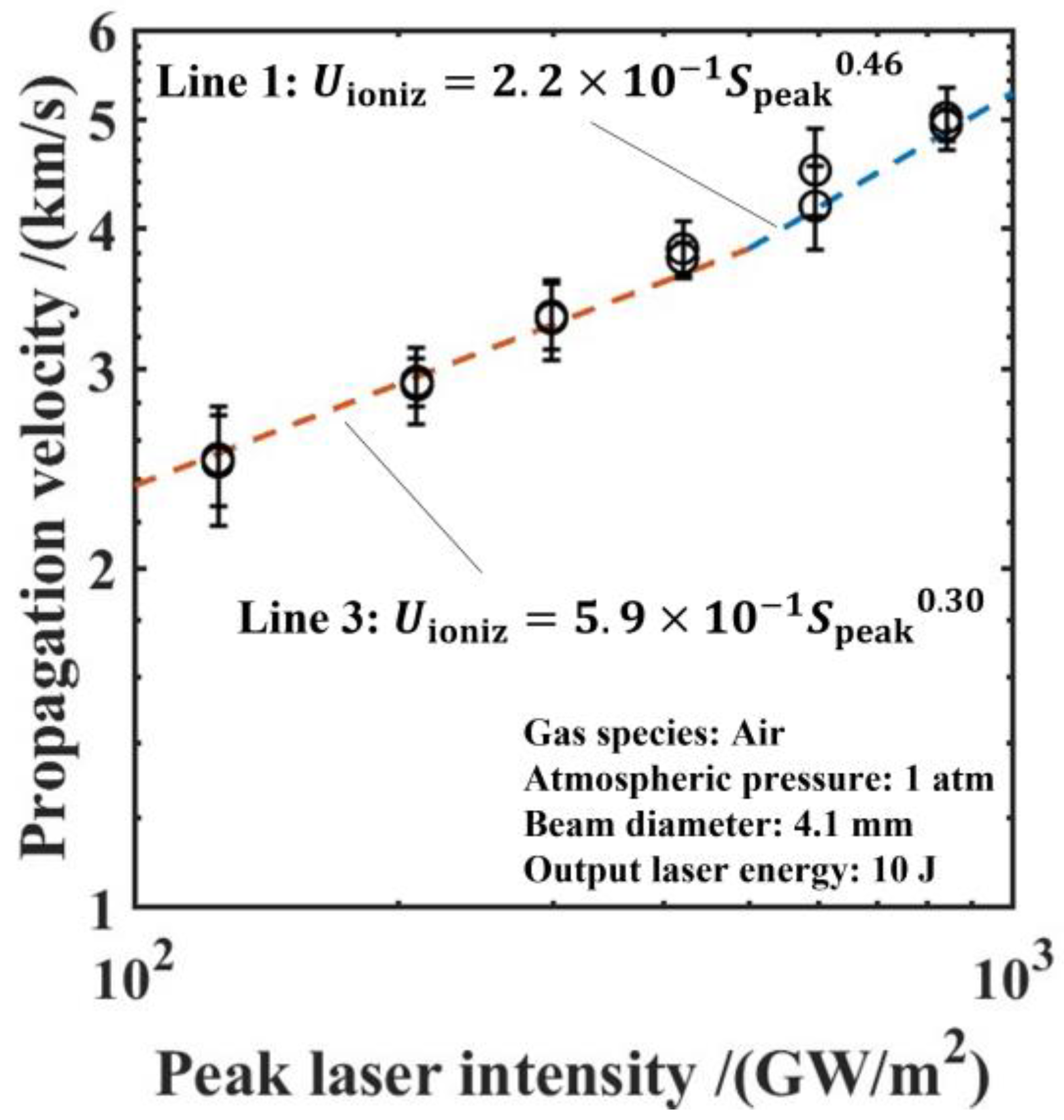
2.1.2. Ionization Wavefront Propagation Velocity
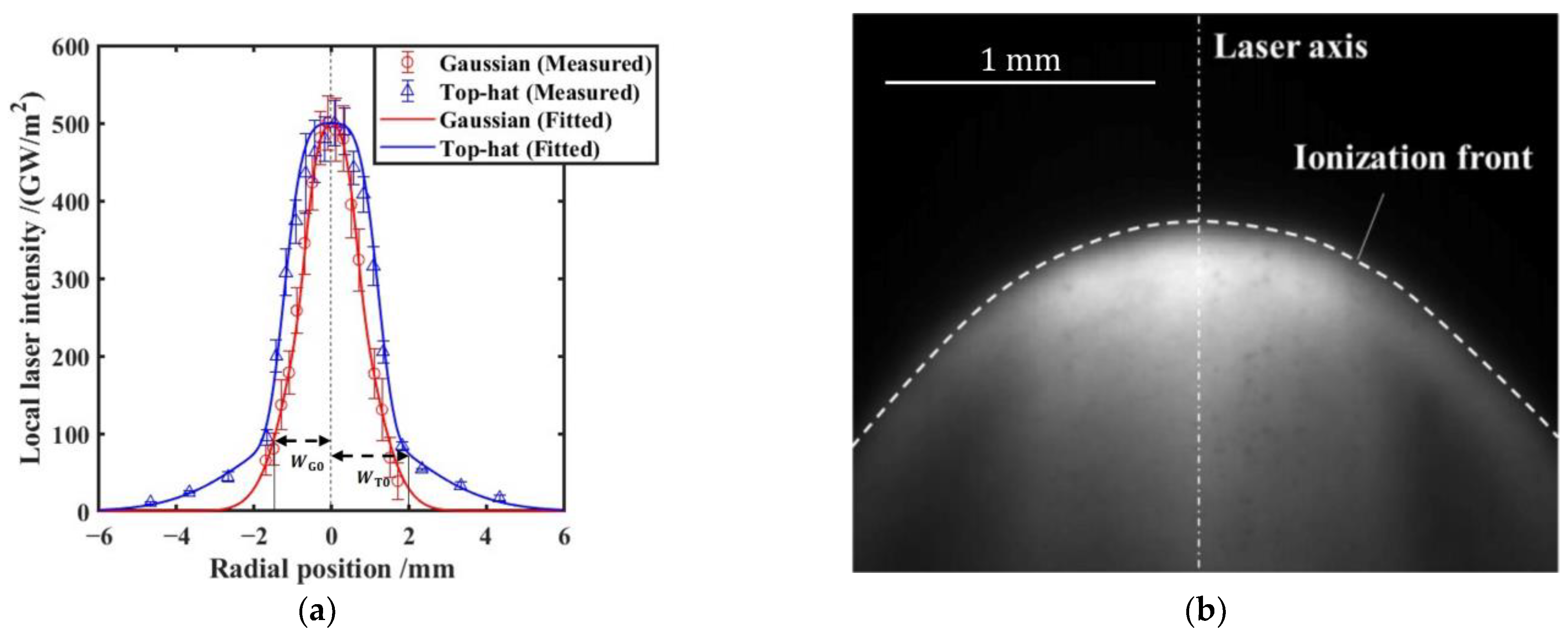
2.1.3. Ionization Wavefront Shape
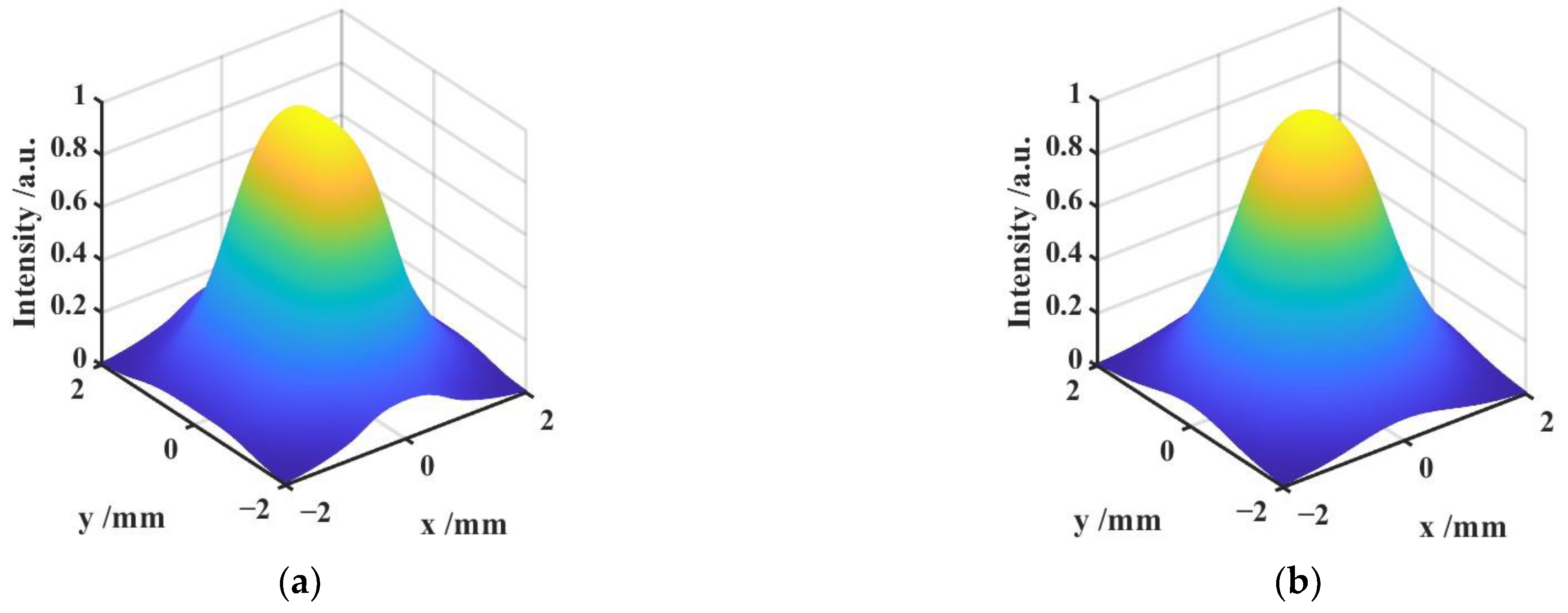
2.1.4. Laser Intensity Calculation
2.2. Governing Equations
2.3. Calculation Conditions
3. CFD Code Validation Based on Pressure History Calculated and Measured Values
3.1. Validation Methods
3.2. Validation Results
4. Calculation Results by Two-Dimensional Axisymmetric CFD
4.1. Calculation Results of the Propagation History of LSD
4.2. Evaluating Effects of Radial Flow from the Central Axis of LSD
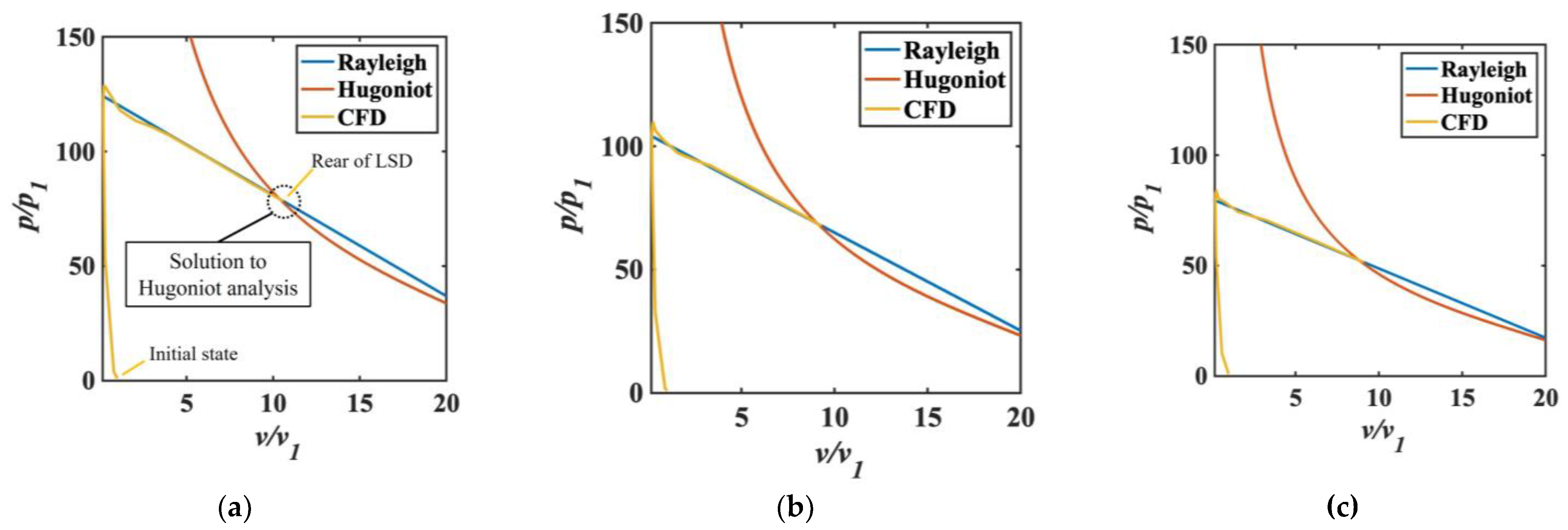
4.3. Hugoniot Relation Considering Radial Flow from the LSD Central Axis
5. Discussion
5.1. Differences in the Radial Flows of Mass, Momentum, and Enthalpy
5.2. Comparison of CJ Velocity Calculated Using the Two-Dimensional Axisymmetric CFD with the Measured Propagation Velocity
6. Conclusions
Author Contributions
Funding
Data Availability Statement
Conflicts of Interest
References
- Kantrowitz, A. Laser Propulsion. Astronaut. Aeronaut. 1971, 10, 74. [Google Scholar]
- Katsurayama, H.; Komurasaki, K.; Arakawa, Y. Feasibility for a Single-Stage-to-Orbit Launch to a Geosynchronous Transfer Orbit by Pulse Laser Propulsion. J. Jpn. Soc. Aeronaut. Space Sci. 2006, 54, 63–70. [Google Scholar]
- Zel’dovich, Y.B.; Raizer, Y.P. Physics of Shockwaves and High-Temperature Hydrodynamic Phenomena; Dover: New York, NY, USA, 2002; pp. 338–348. [Google Scholar]
- Shimamura, K.; Komurasaki, K.; Ofosu, J.A.; Koizumi, H. Precursor Ionization and Propagation Velocity of a Laser-Absorption Wave in 1.053 and 10.6-µm Wavelength Laser Radiation. IEEE Trans. Plasma Sci. 2014, 42, 3121–3128. [Google Scholar] [CrossRef]
- Shiraishi, H.; Fujiwara, T. CFD Analysis on Unsteady Propagation of 1-Dimensional Laser-Supported Detonation Wave Using a 2-Temperature Model. J. Jpn. Soc. Aeronaut. Space Sci. 1998, 46, 607–613. [Google Scholar]
- Raizer, Y.P. Heating of a gas by a powerful light pulse. Sov. Phys. JETP 1965, 21, 1009–1017. [Google Scholar]
- Matsui, K. Study for Laser Parameters Determine the Propagation Velocity and the Wavefront Shape of Laser-Supported Detonation Wave. Ph.D. Thesis, The University of Tokyo, Tokyo, Japan, 2020. [Google Scholar]
- Takeda, R.; Kanda, K.; Matsui, K.; Komurasaki, K.; Koizumi, H. Hugoniot Analysis of Laser Supported Detonation Using Measured Blast Wave Energy Efficiency. J. IAPS 2020, 28, 34–40. [Google Scholar]
- Wang, B.; Komurasaki, K.; Yamaguchi, T.; Shimamura, K.; Arakawa, Y. Energy conversion in a glass-laser-induced blast wave in air. J. Appl. Phys. 2010, 108, 124911. [Google Scholar] [CrossRef]
- Sedov, L.I. Similarity and Dimensional Methods in Mechanics; Academic Press: New York, NY, USA, 1959. [Google Scholar]
- Kinney, G.F. Explosive Shocks in Air; Macmillan: New York, NY, USA, 1962. [Google Scholar]
- Krause, T.; Meier, M.; Brunzendorf, J. Influence of thermal shock of piezoelectric pressure sensors on the measurement of explosion pressures. J. Loss Prev. Process Ind. 2021, 71, 104523. [Google Scholar] [CrossRef]
- Shimamura, K.; Hatai, K.; Kawamura, K.; Fukui, A.; Fukuda, A.; Wang, B.; Yamaguchi, T.; Komurasaki, K.; Arakawa, Y. Structure Analysis of Laser Supported Detonation Waves by Two-Wavelength Mach–Zehnder Interferometer. J. Jpn. Soc. Aeronaut. Space Sci. 2010, 58, 323–329. [Google Scholar]
- Lee, J.H.S. The Detonation Phenomenon; Cambridge University Press: New York, NY, USA, 2008. [Google Scholar]
- Maeda, S.; Sumiya, S.; Kasahara, J.; Matsuo, A. Initiation and sustaining mechanisms of stabilized Oblique Detonation Waves around projectiles. Proc. Combust. Inst. 2013, 34, 1973–1980. [Google Scholar] [CrossRef] [Green Version]
- Kudo, Y.; Nagura, Y.; Kasahara, J.; Sasamoto, Y.; Matsuo, A. Oblique detonation waves stabilized in rectangular-cross-section bent tubes. Proc. Combust. Inst. 2011, 33, 2319–2326. [Google Scholar] [CrossRef] [Green Version]
- Nakayama, H.; Kasahara, J.; Matsuo, A.; Funaki, I. Front shock behavior of stable curved detonation waves in rectangular-cross-section curved channels. Proc. Combust. Inst. 2013, 34, 1939–1947. [Google Scholar] [CrossRef]


| Peak Pressure/atm | Plateau Pressure/atm | |
|---|---|---|
| Calculated value | 27.04 | 2.43 |
| Measured value | 28.57 ± 2.21 | 2.27 ± 0.44 |
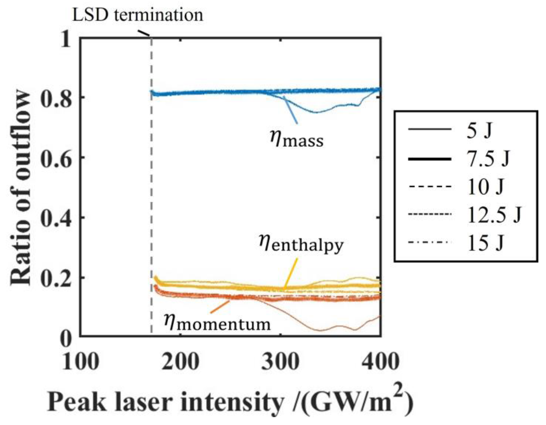
| Average value | 0.82 | 0.13 | 0.17 |
Disclaimer/Publisher’s Note: The statements, opinions and data contained in all publications are solely those of the individual author(s) and contributor(s) and not of MDPI and/or the editor(s). MDPI and/or the editor(s) disclaim responsibility for any injury to people or property resulting from any ideas, methods, instructions or products referred to in the content. |
© 2023 by the authors. Licensee MDPI, Basel, Switzerland. This article is an open access article distributed under the terms and conditions of the Creative Commons Attribution (CC BY) license (https://creativecommons.org/licenses/by/4.0/).
Share and Cite
Sugamura, K.; Kato, K.; Komurasaki, K.; Sekine, H.; Itakura, Y.; Koizumi, H. Hugoniot Relation for a Bow-Shaped Detonation Wave Generated in RP Laser Propulsion. Aerospace 2023, 10, 102. https://doi.org/10.3390/aerospace10020102
Sugamura K, Kato K, Komurasaki K, Sekine H, Itakura Y, Koizumi H. Hugoniot Relation for a Bow-Shaped Detonation Wave Generated in RP Laser Propulsion. Aerospace. 2023; 10(2):102. https://doi.org/10.3390/aerospace10020102
Chicago/Turabian StyleSugamura, Kenya, Kyohei Kato, Kimiya Komurasaki, Hokuto Sekine, Yuma Itakura, and Hiroyuki Koizumi. 2023. "Hugoniot Relation for a Bow-Shaped Detonation Wave Generated in RP Laser Propulsion" Aerospace 10, no. 2: 102. https://doi.org/10.3390/aerospace10020102