Article

A Low-Cost Relative Positioning Method for UAV/UGV Coordinated Heterogeneous System Based on Visual-Lidar Fusion

1
Department of Mechanical Engineering, The Hong Kong Polytechnic University, Kowloon, Hong Kong, China
2
Department of Aeronautical and Aviation Engineering, The Hong Kong Polytechnic University, Kowloon, Hong Kong, China
*
Author to whom correspondence should be addressed.
Aerospace 2023, 10(11), 924; https://doi.org/10.3390/aerospace10110924
Submission received: 30 July 2023 / Revised: 24 October 2023 / Accepted: 26 October 2023 / Published: 29 October 2023
(This article belongs to the Special Issue Intelligent Design, Control and Perception for Unmanned Aerial System)

Abstract

:
Unmanned Ground Vehicles (UGVs) and Unmanned Aerial Vehicles (UAVs) are commonly used for various purposes, and their cooperative systems have been developed to enhance their capabilities. However, tracking and interacting with dynamic UAVs poses several challenges, including limitations of traditional radar and visual systems, and the need for the real-time monitoring of UAV positions. To address these challenges, a low-cost method that uses LiDAR (Light Detection and Ranging) and RGB-D cameras to detect and track UAVs in real time has been proposed. This method relies on a learning model and a linear Kalman filter, and has demonstrated satisfactory estimation accuracy using only CPU (Central Processing Unit)- in GPS (Global Positioning System)-denied environments without any prior information.

1. Introduction

Multi-robot systems, particularly those involving UAVs and UGVs, have gained significant attention in various field robotics applications due to their advantages in terms of reliability, adaptability, and robustness [1]. A heterogeneous multi-robot system refers to a system that consists of different types of robots with different nature, hardware or operating environment. In the case of a UAV-UGV combination, the system includes both UAVs and UGVs, working together towards a common goal [2]. The ground-air configuration of UGV/UAV heterogeneous systems offers a wide coverage within a working space, making it an attractive solution for tasks such as precision farming [1], automated construction [3], search and rescue operations [4], firefighting [5], air quality sensing in smart cities [6], and many others.
A critical aspect of building an effective heterogeneous system is the development of a robust relative positioning method [1]. Relative positioning plays a fundamental role in coordinating the movements and interactions among UAVs and UGVs within the system. Traditional approaches to relative positioning have predominantly relied on visual methods or distance measurement techniques. However, these methods often encounter challenges such as limited accuracy, susceptibility to environmental conditions, and difficulties in handling dynamic scenarios. To address these challenges, the fusion of visual and LiDAR data has emerged as a promising approach in relative positioning for UAV/UGV heterogeneous systems [7,8]. By leveraging the advantages of both sensing modalities, the visual-LiDAR fusion can provide more comprehensive and accurate perception capability for the system. Visual sensors, such as cameras, can capture rich visual information about the environment, including object detection, tracking, and scene understanding. On the other hand, LiDAR sensors can provide precise 3D point cloud data, enabling accurate localization, mapping, and obstacle detection even in low-light or adverse conditions [9,10].
The fusion of visual and LiDAR data has been widely explored in various robotics applications, spanning human tracking [11,12,13], 3D object detection [14,15], and dynamic object tracking [10]. These studies have compellingly showcased the effectiveness of integrating visual and LiDAR sensing for improved perception and localization capabilities. Leveraging the strengths of both modalities, the proposed low-cost relative positioning method for UAV/UGV coordinated heterogeneous systems aims to enhance the system’s reliability, adaptability, and robustness within the operational environment.
In this work, we propose a centralized ground-based perception approach that offloads all sensory modules to the terrestrial robot, thereby reducing the cognitive load on the UAV. In line with existing literatures [16,17], we argue such ground-based precepting method could significantly lighten the burden of the UAV. By considering the constraints of size, weight, and power (SWaP), UAVs can allocate more resources for other mission-critical payloads. Furthermore, it is a feasible method to let the airborne platform have more agile maneuver, as it does not need to take the relative positioning factor into consideration during path planning or trajectory optimization. In addition to the above, for some relative positioning methods, strong computation capabilities might be a requirement. Thus, by allocating this module to UGV, where it could be equipped with more sensors and computing power, the ability to collect and process data could be significantly improved. Last but not least, the UGV can possibly act as a mobile ground station, which can improve communication and data transfer between the UAV and ground control; from time to time, the UGV can provide additional situational awareness by monitoring the UAV’s surroundings during the collaborative mission. The contributions of this work are summarized as follows:
  • A framework that can automatically complete real-time detection and localization of targets without human intervention, using only CPU is proposed. All components in the system are released as open-source packages. https://github.com/HKPolyU-UAV/GTA (accessed on 20 May 2023);
  • Unlike other methods that use a priori target point cloud as a registration reference, this framework combines the advantages of RGB-D and LiDAR to detect and track the desired target without any prior information;
  • LiDAR-inertial odometry (LIO) is integrated into the system to provide accurate altitude estimation for vehicle navigation in GPS-denied environments;
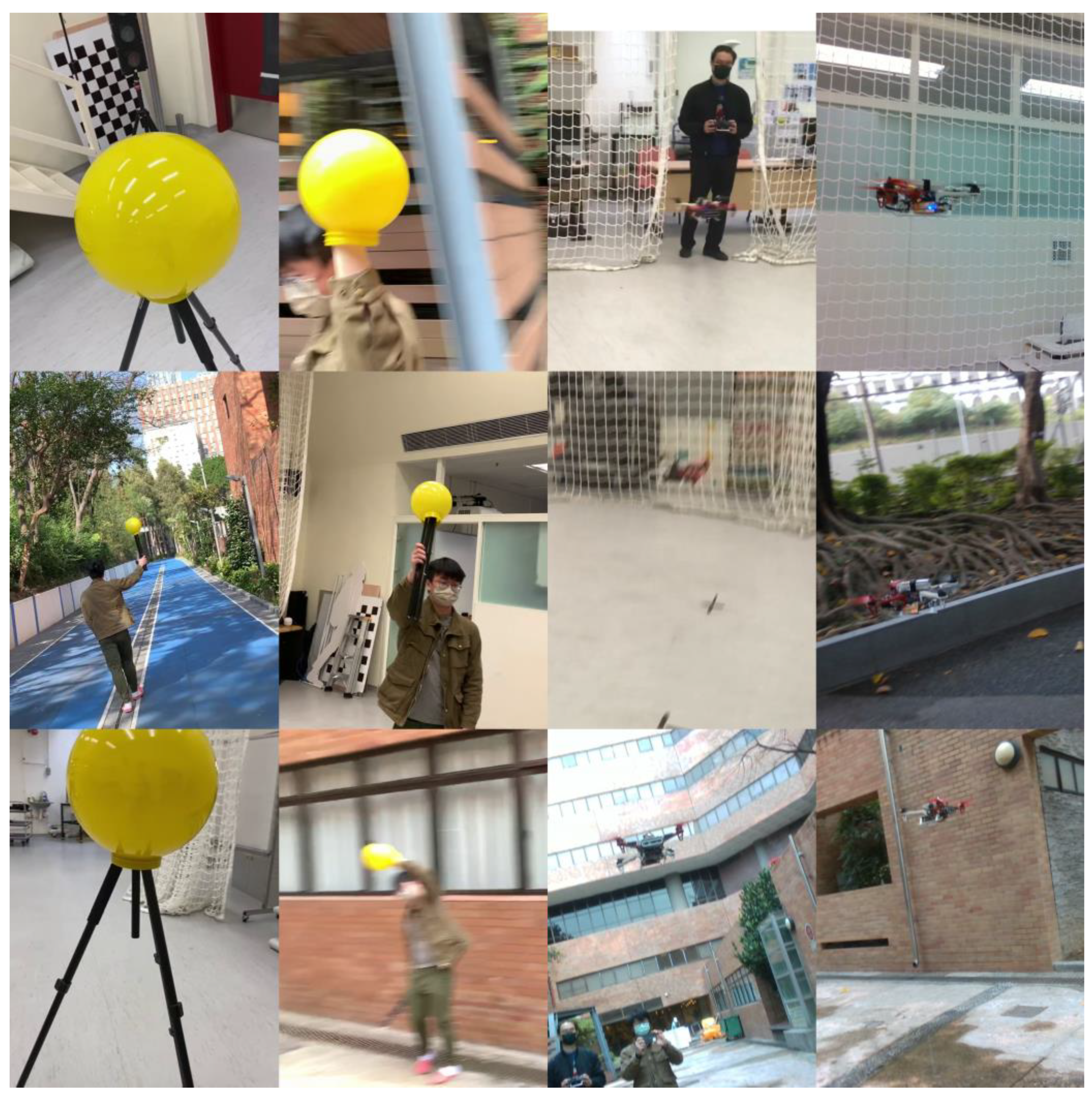
  • Both indoor and outdoor experiments are designed and carried out to illustrate the proposed ideas and methodologies in this work and validate their performance. These indoor and outdoor experiments also serve to provide experimental ideas to other researchers.
The rest of the paper is organized as follows: Section 2 discusses related works. Section 3 introduces the overall software and hardware equipment of the UGV and UAV used in this study. Section 4 provides the methodology of the overall system as well as its implementation details. Section 5 describes the experiments and discusses the results. Section 6 concludes this paper and discusses possible future research directions.

2. Related Works

In this section, a comprehensive review of the existing literature related to relative positioning methods will be presented. This review aims to provide a contextual background for the proposed low-cost relative positioning method based on a visual-LiDAR fusion. The literature review covers topics such as visual-based positioning techniques, LiDAR-based positioning techniques, and visual-LiDAR fusion approaches.

2.1. Visual-Based Positioning Techniques

Visual-based positioning techniques utilize cameras mounted on a vehicle to extract visual information from the environment and estimate their positions. These techniques often involve marker-based and learning-based methods. Several studies have explored the application of visual-based techniques for relative positioning in robot-coordinated systems.
A common approach in visual-based positioning is the utilization of markers or landmarks for position estimation. Hartmann et al. [18] used marker-based video tracking in conjunction with inertial sensors to estimate the 3D position of a vehicle. Eberli et al. [19] focused on a vision-based position control method for MAVs (Micro Air Vehicles) using a single circular landmark. They detected and tracked the circular landmark in the camera images, leveraging its known geometry for position estimation. It is worth noting that the relative position of the marker and the object needs to be calibrated in advance. Once the position of the marker changes during work, it will lead to errors in positioning the object. Some researchers prefer to use LEDs as markers because they are small and easy to detect [16,17]. However, this will bring about another problem. The LED needs to be powered on the object, which will affect the durability of the object itself.
On the other hand, some studies focused on learning-based object detection algorithms for position estimation. Chang et al. [20] focused on the development of a proactive guidance system for accurate UAV landing on a dynamic platform using a visual–inertial approach. Additionally, a mono-camera and machine learning were used to estimate and track the 3D position of a surface vehicle [21]. These studies highlight the potential of learning-based methods in visual positioning tasks and demonstrate their applicability in various domains.
In our work, a learning-based method for object detection was utilized on the visual part. Referring to [22], YOLO-fast-v2 and YOLOv4-tiny became our candidates due to their good performance on CPU-only microcomputers with limited computational power. In practice, we found that the former has shorter running time, but the accuracy is not satisfactory for our work requirements. The latter is slower but has satisfactory accuracy. Our method releases the visual-LiDAR fusion method from tight coupling and allows it to run in parallel, which can greatly reduce the running speed requirements for the visual part. More specific details will be expanded in Section 4.3.

2.2. LiDAR-Based Positioning Techniques

LiDAR-based positioning techniques utilize LiDAR sensors to capture the surrounding environment and estimate the positions of vehicles. LiDAR sensors provide precise 3D point cloud data, enabling accurate localization and tracking. In the context of UAV/UGV coordinated systems, researchers have explored both learning-based and non-learning-based approaches for LiDAR-based positioning.
Non-learning-based LiDAR-based positioning techniques primarily rely on the geometric characteristics of LiDAR data. Quentel [23] developed a scanning LiDAR system for long-range detection and tracking of UAVs. This technique provides a reliable and accurate means of detecting and tracking UAVs, enabling their effective positioning in GNSS (Global Navigation Satellite System)-denied environments. Additionally, Qingqing et al. [24] proposed an adaptive LiDAR scan frame integration technique for tracking known MAVs in 3D point clouds. By dynamically adjusting the scan frame integration strategy, this method improves the accuracy and efficiency of UAV tracking based on LiDAR data, contributing to the precise positioning of UAVs in coordinated systems. However, the geometric properties of the UAV depend on its shape and volume. Without prior information, it is not easy for humans to discover features to detect small UAVs (i.e., DJI F330 drone) relying only on point clouds.
Learning-based LiDAR-based positioning techniques leverage machine learning and deep learning algorithms to extract latent meaningful information from LiDAR data. Qi et al. [25] proposed a point-to-box network for 3D object tracking in point clouds. This method represents objects, including cars, as 3D bounding boxes, enabling accurate and robust tracking using LiDAR data. Their approach achieves satisfactory speed and accuracy on a single NVIDIA 1080Ti GPU, but is limited by the CPU-only situation, which is common in heterogeneous systems for UAVs and UGVs. Inspired by learning-based visual methods for object detection, some researchers have tried to convert point cloud information into images and use one of the most advanced visual detection algorithms, YOLO or CNN, to detect the 2D position of objects. Then, the depth information is given from the point cloud to get the 3D position [8,26]. The proposed UAV tracking system in [8] is consistent with our idea. However, their methods are limited to position estimation based on the output of object detection. Learning-based object detection is time-consuming, which leads to a decrease in overall positioning capabilities or an increase in computational power requirements. Returning object detection to more specialized vision algorithms and freeing 3D object estimation from the constraints of object detection can ensure accuracy while greatly reducing computational costs.

2.3. Visual-LiDAR Fusion Approaches
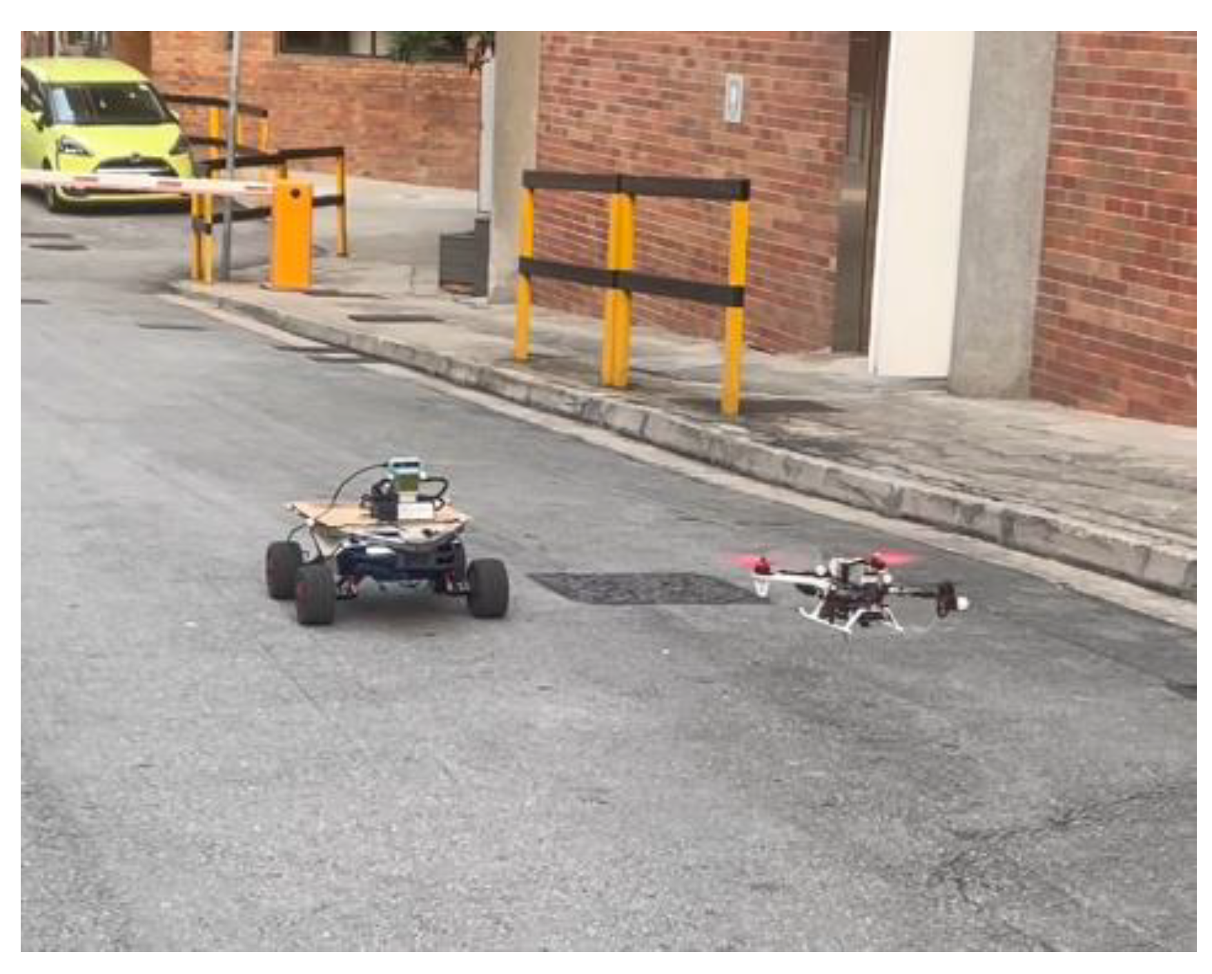
In the realm of UAV/UGV coordinated heterogeneous systems, the integration of visual and LiDAR sensors holds great promise for achieving accurate and robust position estimation. However, each sensor modality has its limitations and strengths. Visual sensors can provide high-resolution imagery and semantic information but are sensitive to lighting conditions and susceptible to occlusions. On the other hand, LiDAR sensors offer accurate 3D point cloud data but struggle with low-texture environments. They are also affected by weather conditions. To overcome these limitations and leverage the strengths of both sensor types, Visual-LiDAR fusion approaches have emerged as a compelling solution.
While ignoring computational power constraints, some learning-based visual-LiDAR fusion frameworks have achieved satisfactory results. Among them, some research frameworks simultaneously extract visual and LiDAR information [10,15], and some explore multi-frame learning using 2D backbone and 3D backbone joint [14]. Different from these, Dieterle et al. [11] presented a sensor data fusion based on a recursive Bayesian estimation algorithm, namely the JPDAF. However, although the detection capabilities of a single sensor can be improved by relying on traditional visual and point cloud data processing methods, accuracy is still a key issue since the RGB information is not utilized to assist object detection.

3. System Overview

This system overview section provides a comprehensive understanding of the hardware platform and software architecture used in our proposed UAV tracking system. This section highlights the key components and their functionalities, emphasizing how they work together to achieve our research objectives. The section is divided into two parts: the hardware platform and the software architecture.

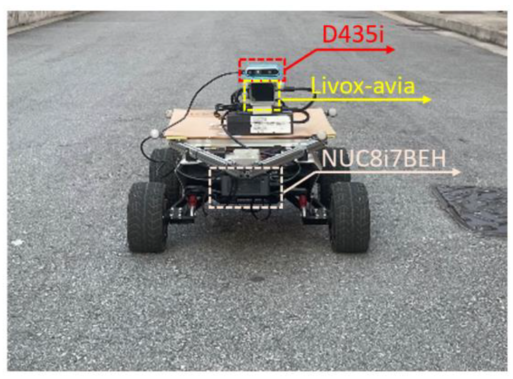
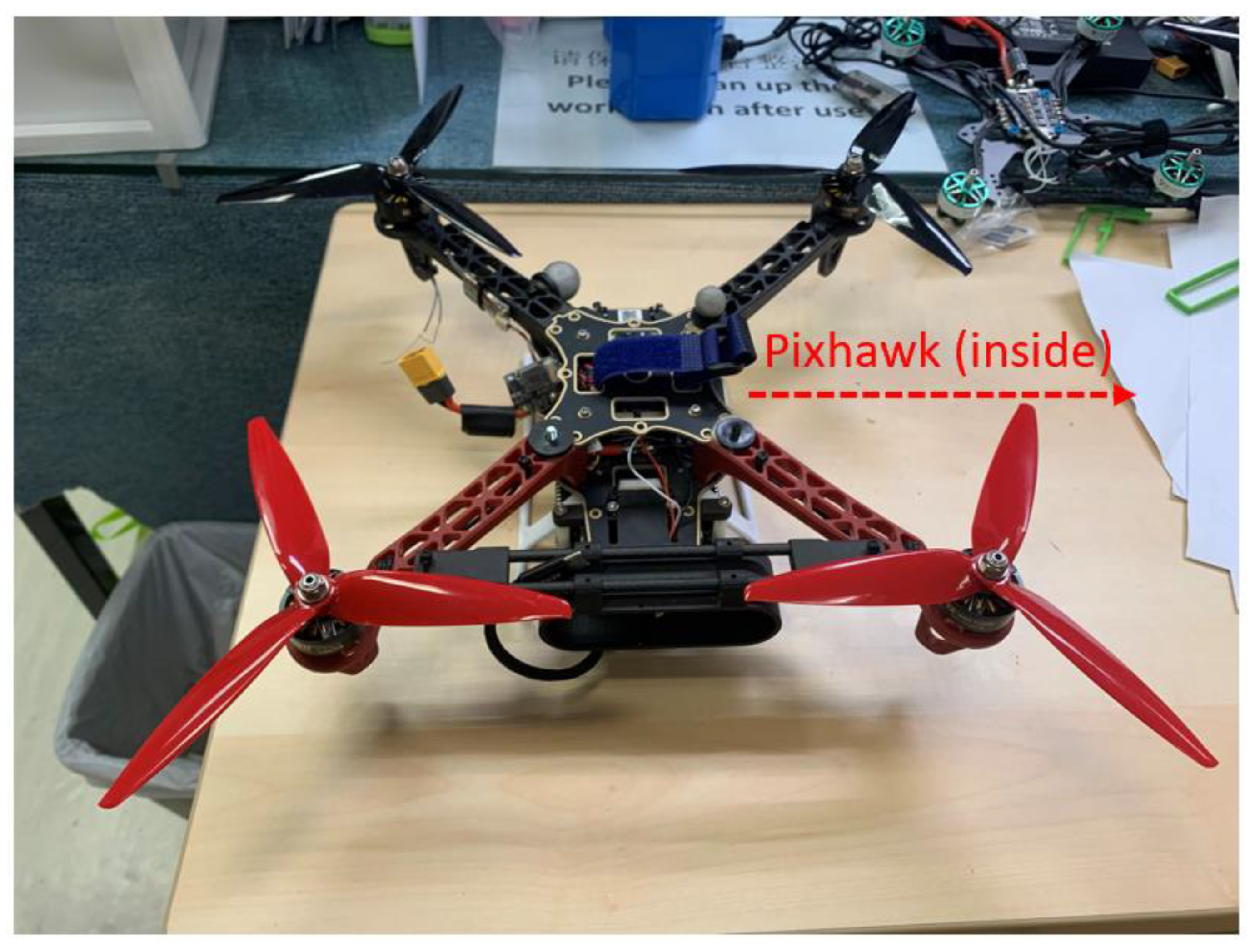
3.1. Hardware Platform

To better demonstrate the effect of the proposed method, a UAV (F330, manual assembly), and a UGV (Scount-mini, produced by AgileX Robotics, Shenzhen, China) will be used for the experiment as shown in Figure 1. The UAV is the object being tracked with no tracking devices other than the equipment itself to maintain flight. In the indoor experiment, a VICON motion capture system was used to locate the UAV and the UGV. The position output for the UAV can be used as the ground truth for the tracking results, and for the UGV, it can provide position feedback for the controllers of the UGV for navigation. The UGV component of the system is responsible for tracking and following the UAV in real time using a combination of the RGB-D camera (D435i, produced by Intel RealSense, US), the 3D LiDAR (Livox-avia, produced by DJI, Shenzhen, China), and an onboard computer (NUC8i7BEH, produced by Intel, US), as depicted in Figure 2. The RGB-D camera captures color and depth information of the surrounding environment, while the 3D lidar provides accurate distance measurements. In the outdoor scene, we apply a LiDAR-inertial odometry (LIO) on the UGV to provide position information for its navigation and path planning.
The UGV utilized in our system is the Scout-Mini UGV, which serves as the mobile platform for UAV tracking. It is a compact and agile UGV capable of traversing various terrains.
For the UAV configuration, we have selected the DJI Flame Wheel 330 (DJI, Shenzhen, China) as the airframe, along with a Pixhawk flight controller mounted on a carrier board as Figure 3 shown. The DJI Flame Wheel 330 is renowned for its stability and maneuverability, making it an ideal choice for our UAV tracking system. The UAV is equipped with four T-motor F80 PRO 1900 KV Brushless Power Motors, which deliver the necessary thrust for flight. The Pixhawk flight controller, an open source and versatile controller, commands the Electronic Speed Controllers (ESCs) to regulate the motor speeds and control the UAV’s movements.
Remarkably, the UAV in our system does not contain any onboard computing unit or tracking sensors for position estimation. Instead, the responsibility of position estimation for the UAV is completely delegated to the UGV.

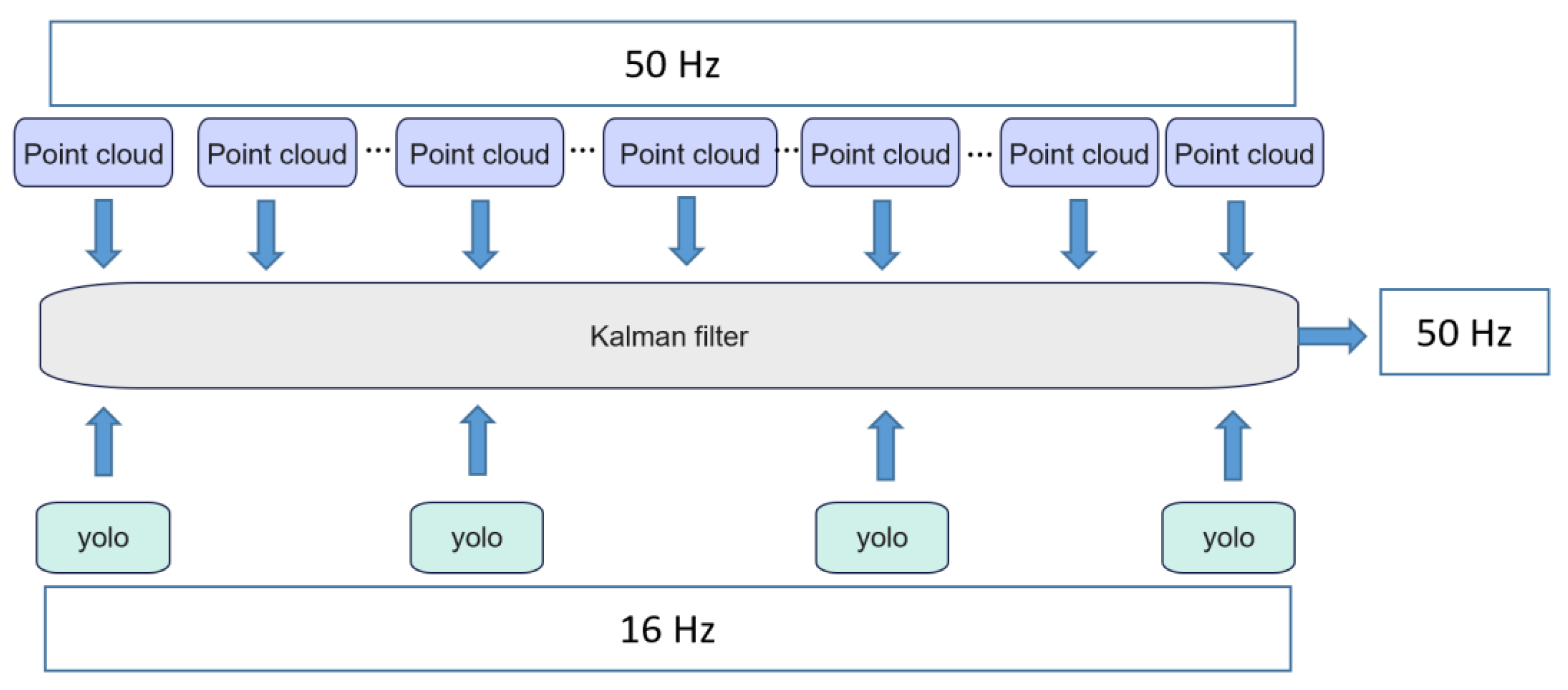
3.2. Software Architecture

The software architecture of the UAV tracking system consists of four main modules: localization, perception, object tracking, and vehicle control. Figure 4 provides an illustration of the software architecture, highlighting the interactions between different modules.
The localization module plays a crucial role in providing accurate position feedback for the autonomous navigation of the UGV. Chen et al. [27] proposed a robust stereo visual inertial pose estimation system. This work contributes valuable insights into developing precise self-localization techniques for robotics and autonomous systems. Depending on the environment, two different localization methods are employed. In indoor experiments, the real-time position information of vehicles is obtained from an external VICON motion capture device. In outdoor scenarios, the UGV utilizes LIO to estimate its position, replacing the VICON system since LIO can utilize point cloud information with a higher information collection frequency and has better robustness and accuracy outdoors compared to visual slam, which is mostly used in indoor environments.
The perception module is responsible for processing data captured by the camera and LiDAR sensors. Prior to system operation, a calibration procedure is performed to determine the 6D pose relationship between these two sensors. The perception module receives RGB images and depth images from the stereo cameras. Utilizing a learning-based object detector called YOLOv4-tiny, the perception module identifies and localizes the UAV within the camera’s field of view (FOV), resulting in a 2D bounding box (2D-BB). Subsequently, a continuous region of interest is computed based on the 2D-BB. This region of interest is utilized to fuse measurements obtained from depth images or 3D point clouds. This fusion process provides accurate 3D position measurements of the UAV relative to the UGV.
The object tracking module utilizes a linear Kalman filter prediction module to process the 3D position measurements obtained from the perception module. The Kalman filter refines the position estimates and generates the desired waypoints for the UGV. Through the vehicle coordinate transformation to the world coordinate system, the UGV determines the position it needs to reach in order to track the UAV effectively.
Finally, the vehicle control module takes the desired waypoint generated by the object tracking module and guides the UGV to reach that particular position. A PID (Proportional-Integral-Derivative) controller is used to generate appropriate control instructions for the UGV, ensuring the precise and robust tracking/following of the UAV. A preliminary user visualization interface was created on an off-board computer using Rviz, a 3D visualization tool in Robot Operating System (ROS). ROS serves as the fundamental framework for information transfer and communication between the various modules in the UAV tracking system.

4. Methodology

In this section, we present the methodology employed in our UAV tracking system. The methodology is divided into four sub-sections, each focusing on a specific aspect of the system’s functionality. We begin with discussing the extrinsic calibration between the stereo camera and LiDAR, which is essential for accurate object detection and position estimation. Next, we delve into the two-dimensional (2D) object detection module, followed by the three-dimensional (3D) position estimation module. Finally, we provide an overview of the 3D tracking algorithm used to track the UAV’s position over time and guide the UGV’s movements.

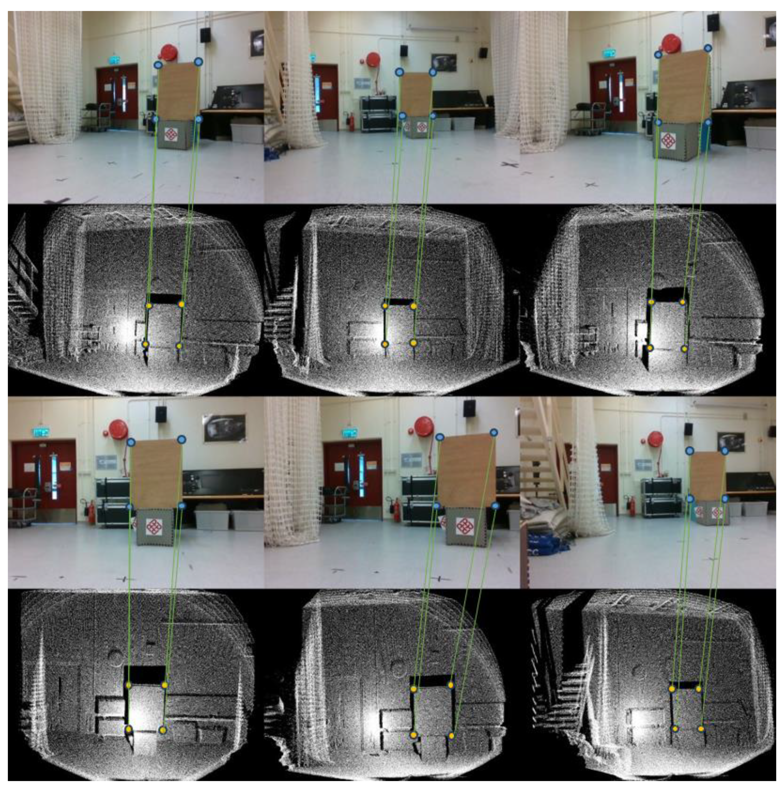
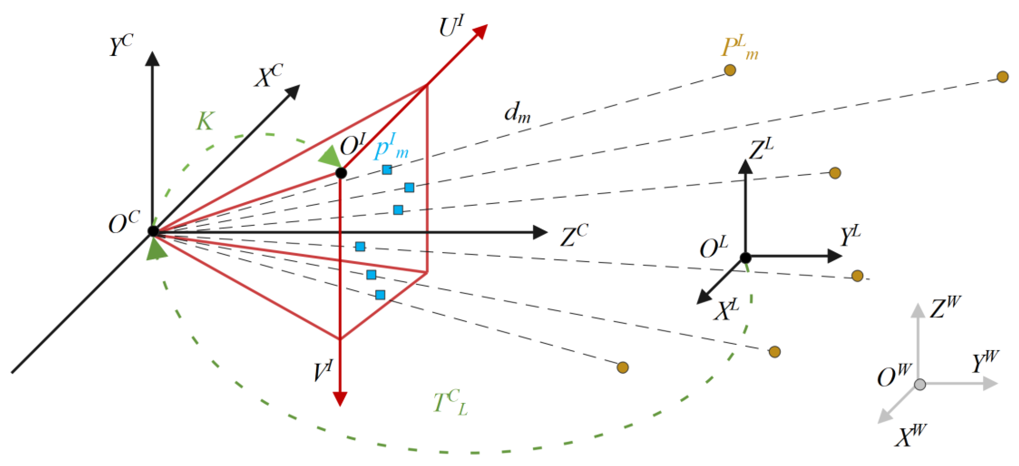
4.1. Extrinsic Calibration between Camera and LiDAR

In order to fuse the data from LiDAR and RGB camera, it is necessary to calibrate them to ensure that their coordinate systems are aligned. The D435i contains an RGB camera and a depth camera whose intrinsic and extrinsic parameters are already known, which means that if the extrinsic parameters of the LiDAR and RGB cameras are obtained, the relative positions and rotations of the coordinate systems of these sensors are also available. This calibration process involves determining the transformation matrix between the LiDAR and camera coordinate systems. In this section, the calibration process between the LiDAR and RGB camera is discussed.
There are several approaches to calibrating LiDAR and RGB camera, but one popular method is to use a calibration target with known geometry. A planar board is the most commonly used, as shown in Figure 5. The corners of the board can be detected in both the LiDAR and RGB images, and their correspondence can be established. This allows us to compute the transformation matrix that maps points in the LiDAR coordinate system to the camera coordinate system based on the solution for a Perspective-n-Point (PnP) problem [28].
The PnP problem can be simply summarized as follows: Given a set of n 3D points in a reference frame and their corresponding 2D image projections and calibrated camera intrinsic parameters, the 6 degrees-of-freedom (DOF) pose of the camera relative to the reference frame in the form of rotation and translation can be determined. As shown in Figure 6, there are four coordinate systems belonging to the camera, the imaging plane of the camera, the LiDAR, and the real world, in which the coordinates are distinguished by the superscripts C (camera), I (image plane), L (LiDAR) and W (real world), respectively. For instance, p I m is the pixel coordinate corresponding to a point in the real world on the camera imaging plane, while P L m is the corresponding 3D coordinate in the LiDAR frame.
Suppose enough 3D-2D corresponding point pairs have been collected, where the 3D coordinate of a point is P L m and the 2D pixel point is p I m .
P L m = X m Y m Z m T ,
p I m = u m v m 1 T .
According to the pinhole camera model, the relationship between the corresponding 3D point position and the pixel position can be established as follows:
d m p I m = K T C L P L m ,   T C L S E 3 ,
where d m is a scalar representing the distance between the point and the origin of the camera frame (OC) in the real world, and K stands for the intrinsic parameter matrix of the camera, which converts the camera frame to the pixel frame. Usually, there is a distortion matrix used to correct the distortion generated during the imaging process of the camera. However, the stereo camera D435i used in this study has been corrected at the factory. Therefore, it is not considered in this paper. T C L is the extrinsic parameter matrix converts the 3D point to the 2D point, which we want to find out through the measurement of 3D-2D point pairs. In particular, T C L is a 4-by-4 matrix, P L m is a 3-by-1 vector, and K is a 3-by-3 matrix. In order to make the matrix multiplication on the right side of Equation (3) hold true, P L m is augmented to 4-by-1 during the actual calculation. Thus T C L P L m is a 4-by-1 vector. Then, take its first three dimensions yields, the 3-by-1 vector, and multiply it with K . The result should be a 3-by-1 vector whose dimension is equal to the result on the left side.
If an initial value of T C L is given, which is highly likely to be different from the true value, by using Equation (3), a reprojection error e m can be obtained:
e m = p I m 1 d m K T C L P L m ,
Each point pair can be calculated for a reprojection error based on Equation (4). By adding them up, a least squares problem can be constructed:
T C * L = a r g m i n T C L 1 2 m = 1 n e m 2 2 .
There are many ways to optimize Equation (5), such as the first-order gradient method, the second-order gradient method, the Gauss–Newton method and the Levenberg–Marquardt method, etc. Here, the Levenberg–Marquardt [29] method is used, which can be implemented by directly calling the function in the OpenCV library [30]. In particular, the selection of the initial value of T C L should consider taking a value near the true value, which is to prevent the solution of Equation (5) from falling into a local optimum. Here, a raw value measured in the Solidworks 3D model interface (a solid modeling computer-aided design (CAD) and computer-aided engineering (CAE) application published by Dassault Systèmes) is adopted.

4.2. Two-Dimensional (2D) Object Detection

To perform 2D object detection in real time, we utilized the You Only Look Once (YOLOv4-tiny) object detection algorithm, which is an improved version of the original YOLO algorithm proposed by Redmon et al. [31]. YOLOv4-tiny is a lightweight version of the YOLOv4 [32] algorithm, specifically designed for real-time object detection tasks on embedded devices with limited computational resources. Using this detector to obtain the 2D bounding box corresponding to the object and establish a custom data set to train the YOLOv4 model will be mainly discussed in this section.

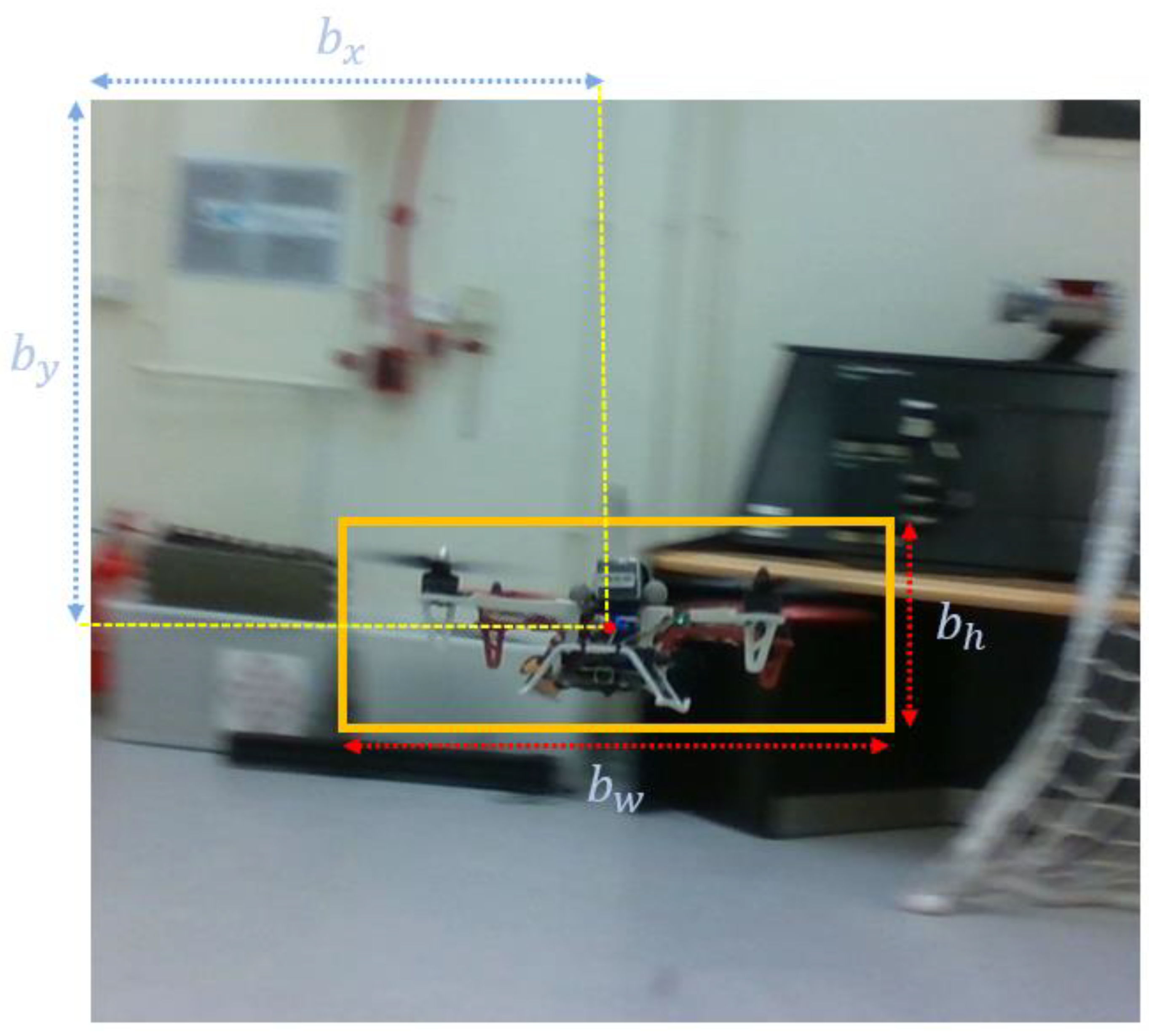
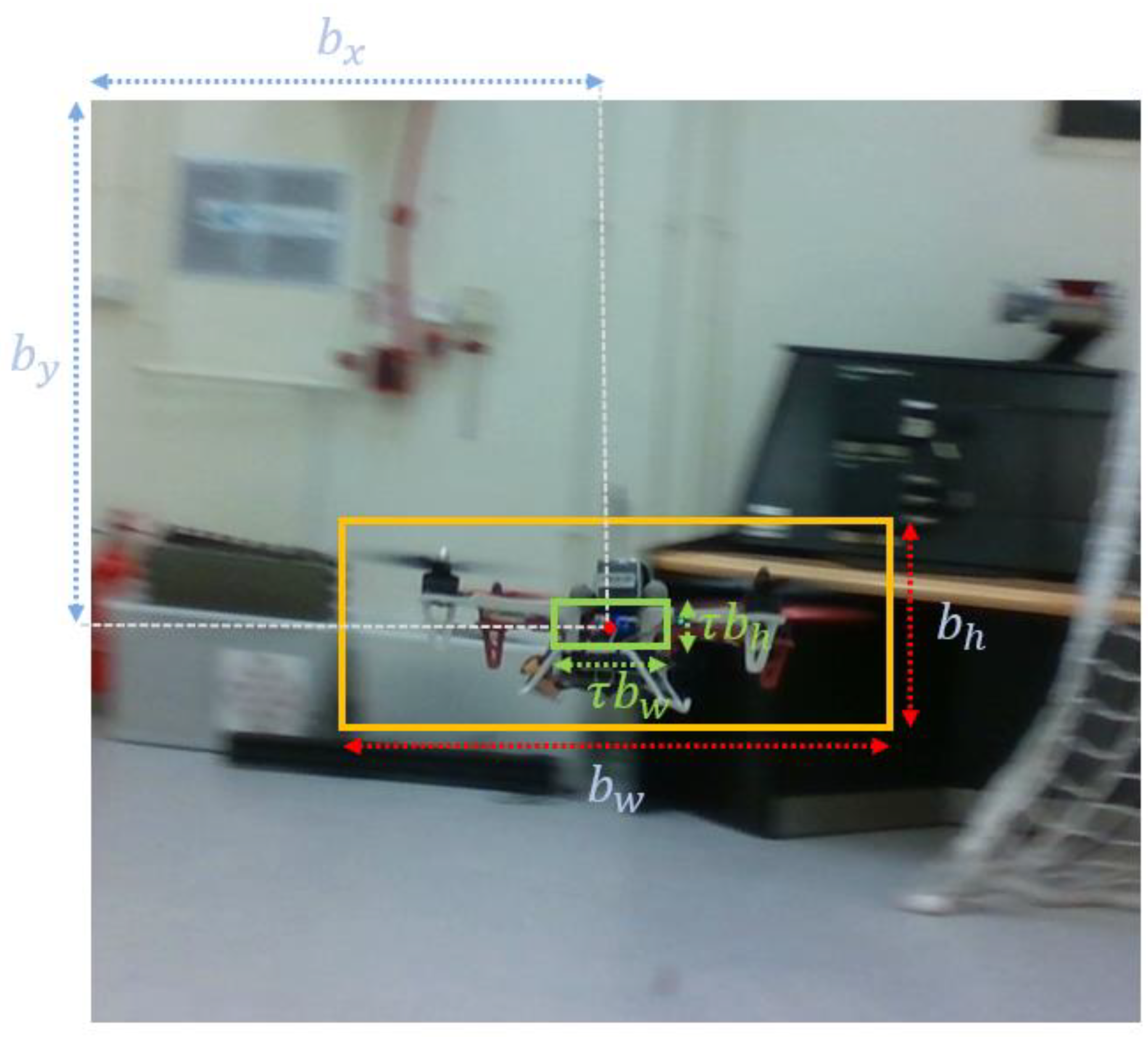
4.2.1. Two-Dimensional (2D) Bounding Box Prediction

According to Redmon and Farhadi’s work [33], an anchor-based method is used to maximize the intersection over union (IOU) between the ground truth box and the bounding box. Taking the image stream from the camera as the input, each image is resized to a fixed size. Then, the input image is passed through a deep neural network (backbone), a modified backbone (CSPDarknet53-tiny), to extract features at different scales. The feature maps obtained from the backbone are then processed by several prediction layers. Based on these maps, by using k-means clustering, we can generate the anchor boxes that are predefined boxes of different sizes and aspect ratios being placed at different positions on the image. These anchor boxes are used to predict bounding boxes in a one-to-one way with following equations:
b x = σ t x + c x ,
b y = σ t y + c y ,
b w = p w e t w ,
b h = p h e t h ,
where
  • b x , b y , b w , and b h are parameters for the bounding box, with x representing the position of the center (on the image plane), y representing the position of the center, w representing the width, and h representing the height, respectively;
  • t x , t y , and t w , and t h are the predicted values from the network for the bounding box, which is utilized to compute the parameters for the bounding box;
  • p w and p h are the prior width and height for the bounding box;
  • σ is the sigmoid function applied to constrain the offset range between 0 and 1;
  • Figure 7 shows an illustration of the bounding box predicted by YOLOv4-tiny.

4.2.2. Custom Training Dataset Establishment

Establishing a custom training dataset is a crucial step in fine-tuning the YOLOv4-tiny model for detecting both the UAV and yellow bulb objects in our specific scenario. The dataset should contain a representative sample of images that capture the range of variations in the environment and conditions under which the UGV is required to track the objects.
The dataset was established through a two-step process. First, we manually selected frames from the video footage captured by the UGV using D435i, which contains the UAV in different orientations and locations, and is representative of the scenarios that the UGV would encounter during dynamic UAV tracking. Next, the open source annotation tool LabelImg [34] is was utilized to annotate the dataset by drawing bounding boxes around the UAVs and assigning them the corresponding class labels. The annotated images were split into training and validation sets with a ratio of 4:1. The training set was used to fine-tune the pre-trained YOLOv4-tiny model, while the validation set was used to evaluate the model’s performance during training and determine when to stop training to avoid overfitting. Total 9000 images were utilized to establish the dataset, where each object (the UAV/the yellow bulb) had 2000 training images and 500 validation images, while 4000 background images without target objects were used to train the model to learn the scenario with no objects in the scene, thereby reducing false positive (FP) results and improving the accuracy of the model. To improve the robustness of the model, we also applied data augmentation techniques, such as random scaling, flipping, and rotation, to the training images, as shown in Figure 8. This helped to increase the diversity of the dataset and reduce the likelihood of overfitting.

4.3. Three-Dimensional (3D) Position Estimation

After obtaining the 2D bounding box of the UAV in each frame, we used it to generate a region of interest (ROI) in the depth image and point clouds captured by the RGB-D camera and LiDAR, correspondingly. The ROI can help to extract the depth information of the object. Then, the measurement of 3D position was obtained. Then, a Kalman Filter was applied to track the object.

4.3.1. Depth Assignment Based on 2D Bounding Box

The ROI is defined as a rectangular region that is scaled down by a certain ratio relative to the center of the bounding box, which is to ensure that all the extracted depth information comes from object pixels rather than the background. From Section 4.2.1, we used 4 parameters to describe a 2D bounding box R b b :
R b b = b x b y b w b h ,
By applying a scale factor τ to R b b , the ROI R I can be obtained:
R I = b x   b y   τ b w     τ b h ,
where τ is set to 0.25 as an empirical value in the experiments. The ROI on the image plane is shown in Figure 9.
The aligned depth image eliminates invalid depth values in the corresponding ROI and averages the remaining effective pixels to represent the depth in the ROI, that is, the depth of the object from the stereo camera. The calibrated LiDAR can use Equation (3) to convert the 3D point cloud coordinates into the 2D pixel coordinates of the corresponding image and obtain the depth value of the corresponding pixel. Similarly, after removing the outlier, the depth of the ROI can be obtained by averaging the remaining pixel depth values. In case no point cloud data of the UAV is captured by the LiDAR, we can use the depth image to compensate for depth information. Finally, based on the pinhole camera model, the depth value is used to determine its scale, and the 3D position measurement value in the camera frame of the object is obtained.

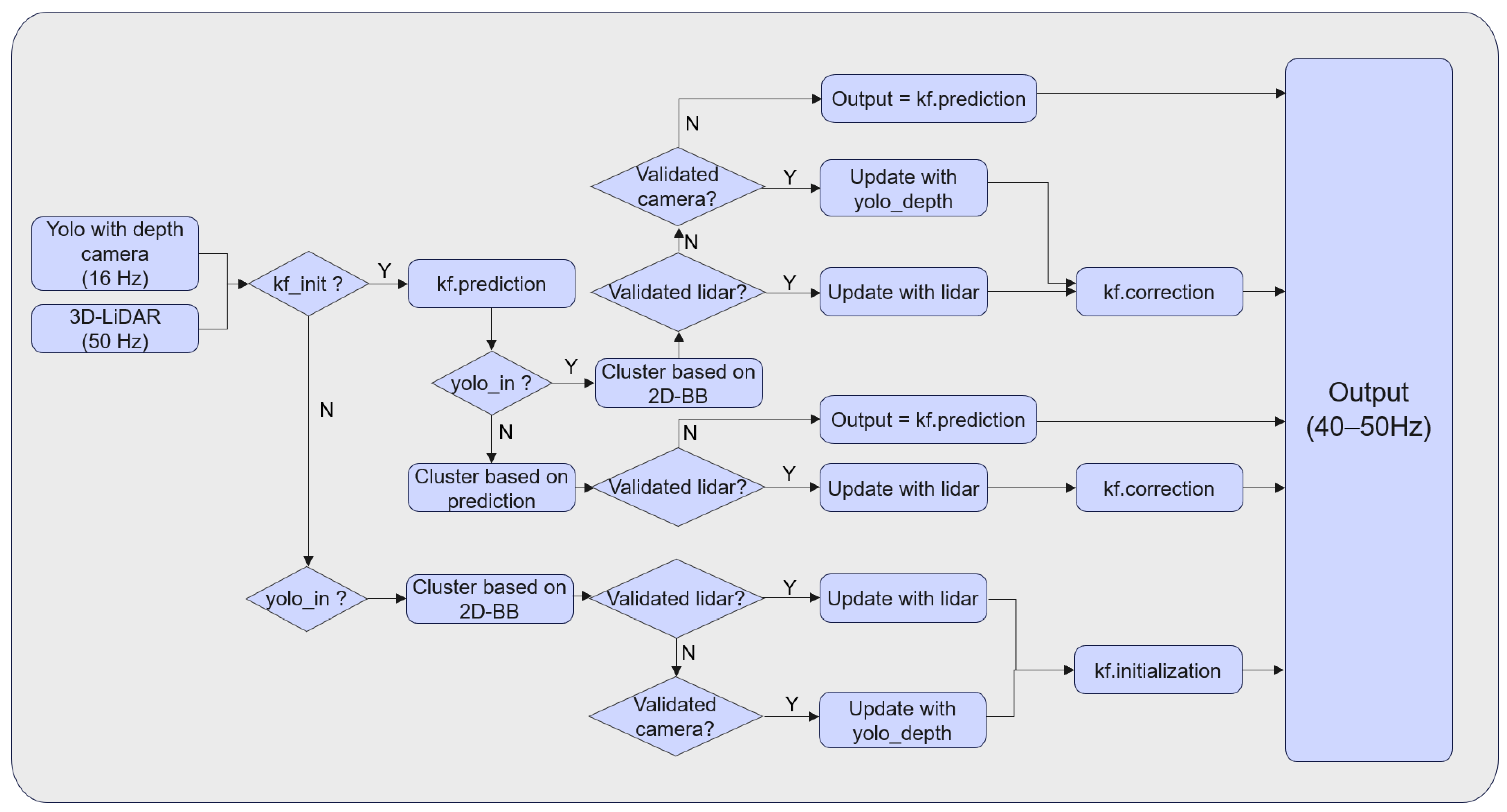
4.3.2. Tracking by Kalman Filter

The linear Kalman filter is a mathematical tool used to estimate the state of a system based on a set of noisy measurements. In the context of the 3D position estimation, the system refers to the position of the UAV in 3D space, while the noisy measurements refer to the 3D position of UAV that is computed by the 2D bounding box and depth information obtained from the RGB-D camera and the LiDAR. The Kalman Filter was used to predict the UAV’s position based on its previous position and velocity, and to correct the prediction using the new measurements obtained from the sensors.
Firstly, we defined the state vector of the object at time k , which consists of the 3D position in the camera frame and the corresponding velocity, which is a 6-by-1 vector.
s k = p x p y p z v x v y v z T ,
In the linear Kalman filter, two assumptions need to be satisfied: (1) the state at the current moment is linearly related to the state at the previous moment, and the measurement at the current moment is linearly related to the state at the current moment; and (2) all states, measurements, and noises follow Gaussian distribution. Then, we can obtain the state equation and observation equation of the system:
s k = A s k 1 + B u k 1 + w k ,
m k = H s k + n k ,
Specifically,
A = 1 0 0 Δ t 0 0 0 1 0 0 Δ t 0 0 0 1 0 0 Δ t 0 0 0 1 0 0 0 0 0 0 1 0 0 0 0 0 0 1
H = 1 0 0 0 1 0 0 0 1 0 0 0 0 0 0 0 0 0
m k = p x p y p z
where A is the state transition matrix, B u k 1 is the input that is equal to zero in our system, w k is the process noise, m k is the measurement, H is the mapping matrix from the state space to the measurement space, and n k is the measurement noise. Kalman filtering can be divided into two processes: prediction and correction.
Prediction:
s ^ k = A s ^ k 1 ,
P k = A P k 1 A T + Q ,
Correction:
K k = P k H T H P k H T + R 1 ,
s ^ k = s ^ k + K k m k H s k ,
P k = 1 K k H P k ,
in which Q and R are the covariance matrices of noises w k and n k . Q and R are fixed and set by ourselves empirically. P k is the error covariance matrix.
Suppose we have the optimal state ( s ^ k 1 ) at time k 1 and its corresponding covariance matrix ( P k 1 ). By applying Equations (18) and (19), the prediction of the state ( s ^ k ) at k and its corresponding covariance matrix ( P k ) can be obtained. Then, the Kalman gain ( K k ) is computed by using Equation (20). The optimal state ( s ^ k ) at time k can be acquired in Equation (21) with K k and s ^ k . Finally, Equation (22) corrects the corresponding covariance matrix ( P k ) of the state at time k for the calculation of next time step ( k + 1 ). Through this iterative process, the 3D position in camera frame of the UAV can be tracked all the time, even if the sensor fails in a short period of time.
The tracking of the UAV’s 3D position is accomplished using a Kalman filter, as depicted in Figure 10. The Kalman filter takes the output of the YOLO detector with depth information (operating at a frequency of 16 Hz) and the 3D point cloud data from the 3D LiDAR (operating at a frequency of 50 Hz). By decoupling lidar and visual information processing, the output frequency can be comparable to that of lidar, close to 50 Hz, at a low computational cost. Figure 11 presents the details of Kalman filter processing.
During the initialization phase of the Kalman filter, the first measurement of the UAV’s position was used as the prior state. To ensure the accuracy of the tracking results, a strict criterion was applied to determine the validity of the measurement. Given the higher accuracy of the LiDAR, the depth information was given priority. Only when a correct 2D bounding box (2D-BB) of the UAV was obtained from the YOLO detector was the point cloud of the UAV extracted based on the 2D-BB and the centroid coordinate of the point cloud considered as the position measurement. If this measurement met the validity criterion, it was saved as the prior state. Otherwise, the depth information from the depth camera was considered. If the depth camera measurements also failed to meet the criterion, indicating that the information from the current frame is invalid, another frame will be considered.
Once the initialization was complete, for each new frame, the Kalman filter predicted the position based on the last state of the UAV. Subsequently, the point cloud data were primarily used to cluster the measurements based on the predicted state without relying on visual information. However, if the output from the YOLO detector was available, the point cloud of the UAV was extracted based on the 2D-BB obtained from YOLO instead of relying solely on the predicted state. As before, LiDAR measurements took precedence over depth camera measurements. The state of the UAV was then corrected using the validated measurements and output to other modules. In cases where all measurements failed, the predicted state was the output. This ensures that the frequency of the output closely matches the highest frequency of the two sensors even under the no-GPU limitation, which is 50 Hz.
It is important to note that if 100 consecutive measurement failures occur, the Kalman filter is re-initialized to ensure the accuracy of the output. However, the initialization process is time-consuming due to the stringent criteria for success, which are imposed to guarantee accuracy in the tracking results.

4.4. Overview of 3D Tracking Algorithm

The overall tracking process is shown in Algorithm 1. The system receives the RGB image from the camera and uses a learning-based detector to recognize the image and detect the presence of the target object (in this case, a UAV and a yellow light bulb). If the target object is identified, its 2D bounding box is output, and the ROI is calculated. The depth image or point cloud data will calculate the distance of the target object relative to the sensor based on ROI, and for accuracy considerations, point cloud data from LiDAR will be given priority. When LiDAR fails, depth images are used to compensate for depth information. Finally, the pinhole camera model is used to recover the 3D position measurement of the target object in the camera frame. In order to prevent the detector from misidentifying, only when the confidence value of the detected object is greater than a threshold will the object be regarded as the target object. Empirically, the threshold is set to 0.9. The valid measurements are sent to the Kalman filter configured to track the 3D position of the object. The correction value of each iteration will be regarded as the actual 3D position of the object at the current moment.
Algorithm 1. 3D Tracker Based on Learning Model and Filter
Notation: RGB image set C , depth image set D , LiDAR point cloud P , object state s ^ k , measurement m k , Kalman filter KF
Input:
 RGB image C
 depth image D
 point cloud P
Output: the actual state of the object at the current moment s ^ k
While true do
  2D-Detector.detect( C , D )
  if confidence value > 0.9 then
     m k = Detector.output()
  end if
end while
While true do
  if object detected then
    update m k by fusing P and Detector.output()
    if KF initiated then
      KF.predict()
      if validated measurement then
         s ^ k = KF.correct( m k , KF.predict())
        continue
      else
         s k = KF.predict()
        continue
      end if
    else
      initiate KF
      continue
    end if
  else
    if KF initiated then
      KF.predict()
      point cloud process( P )
      if validated measurement then
         s ^ k = KF.correct( m k , KF.predict())
        continue
      else
         s k = KF.predict()
        continue
      end if
    else
      continue
  end if
end while

5. Results and Discussion

In this section, we present the experimental results to validate the proposed system for tracking a dynamic UAV in real time using a LiDAR and RGB-D camera mounted on a UGV. The experiments are divided into three parts. Firstly, we evaluate the performance (accuracy and speed) of the trained YOLOv4-tiny model based on a custom dataset designed for the proposed scenario of two objects. Secondly, we conduct an indoor experiment by utilizing the motion captured devices (VICON) to verify the accuracy of 3D position estimation. Finally, we conduct a field test in an outdoor environment with an integrated LiDAR-inertial odometry to demonstrate the effectiveness of the proposed system.

5.1. Training Result for YOLOv4-Tiny Model on Custom Dataset

A good performance for 2D object detection is a prerequisite for accurately estimating the 3D position of the target object. In order to obtain good training results, we compared the performance of the trained model on the dataset in terms of different input size. The input sizes are of 320 × 320; 416 × 416; 512 × 512; and 608 × 608 resolutions, respectively. In the training results shown in Table 1, it can be seen that the training model with an input size of 608 × 608 has the highest accuracy and whose mean average precision (mAP) is 98.63% with an intersection over a union threshold of 0.5 ( A P 50 ), while the highest speed is shown with the size of 320 × 320 under the same backbone according to Table 2. Notably, two backbones (i.e., CSPDarknet-53-tiny and NCNN) were used to run the trained model to find the best performance for speed because in the proposed system the requirement of real-time tracking takes higher priority. Obviously, the higher input sizes give better accuracy, but also lower speed, which is in line with our expectation. In the trade-off between accuracy and speed, we chose 416 × 416, which is the fastest while still meeting acceptable accuracy. NCNN was finally chosen as the backbone running on the UGV due to its lightness, which is a high-performance neural network optimized for mobile platforms and open sourced by Tencent Youtu Lab.
The effect of data without any objects (background images) was also considered in the experiments. The datasets with/without background images are trained separately, and the results of resolution are shown in Table 3. It can be seen that the accuracy of the training results with background images trained is significantly improved by reducing the false positive situations (see Section 4.2.2).
Finally, 2D detection is applied in both indoors and outdoors environments, and good results are obtained to verify its robustness.

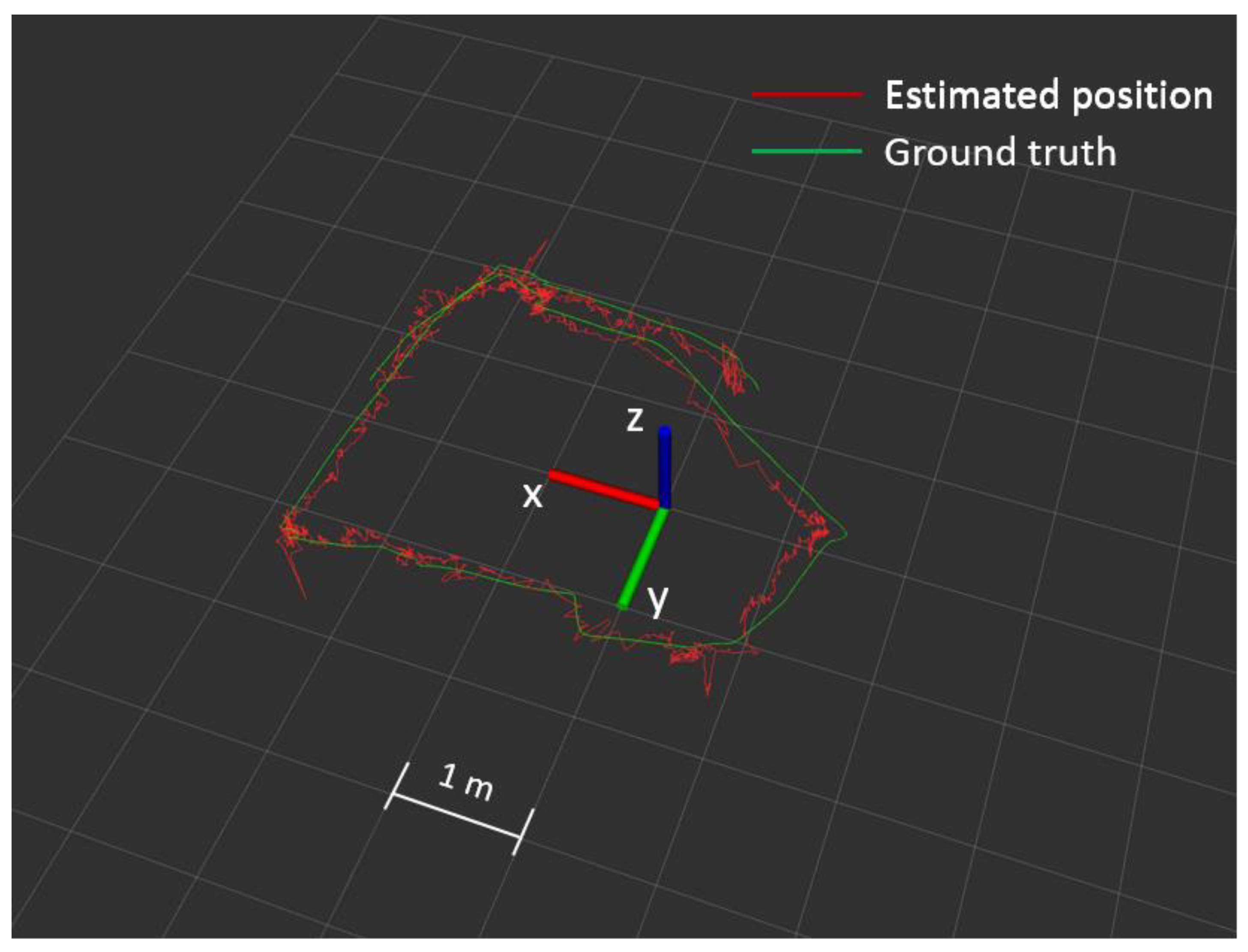
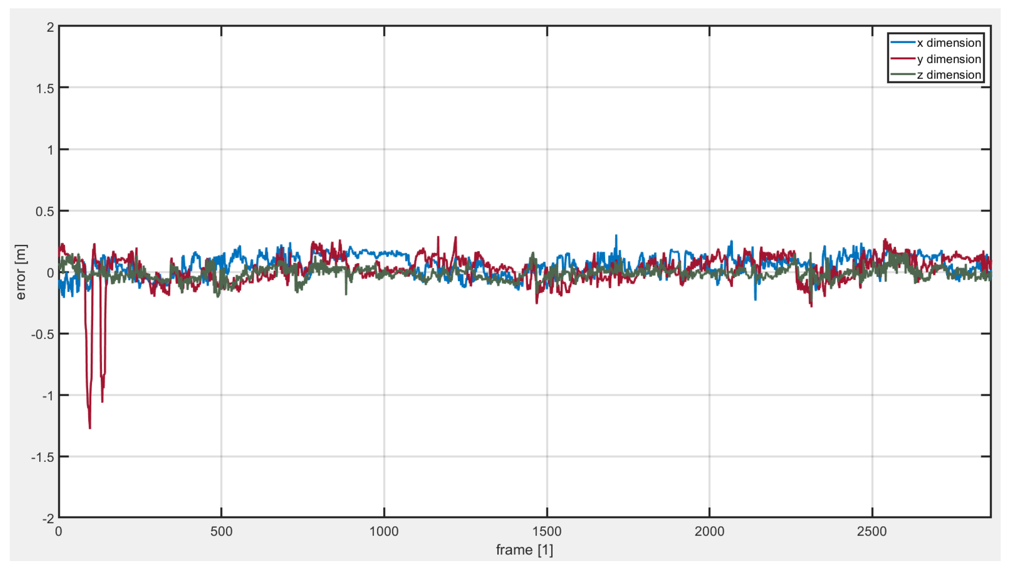
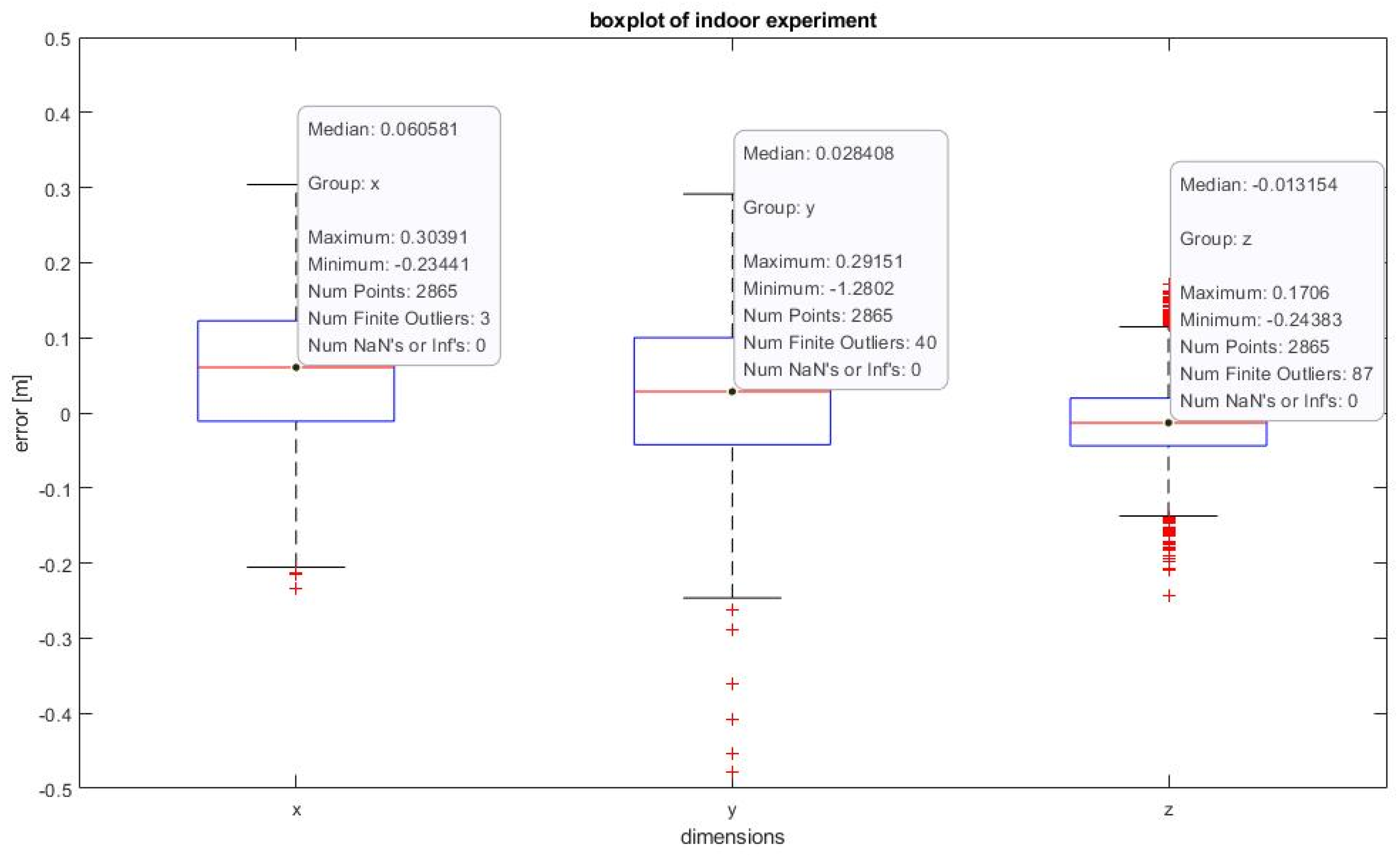
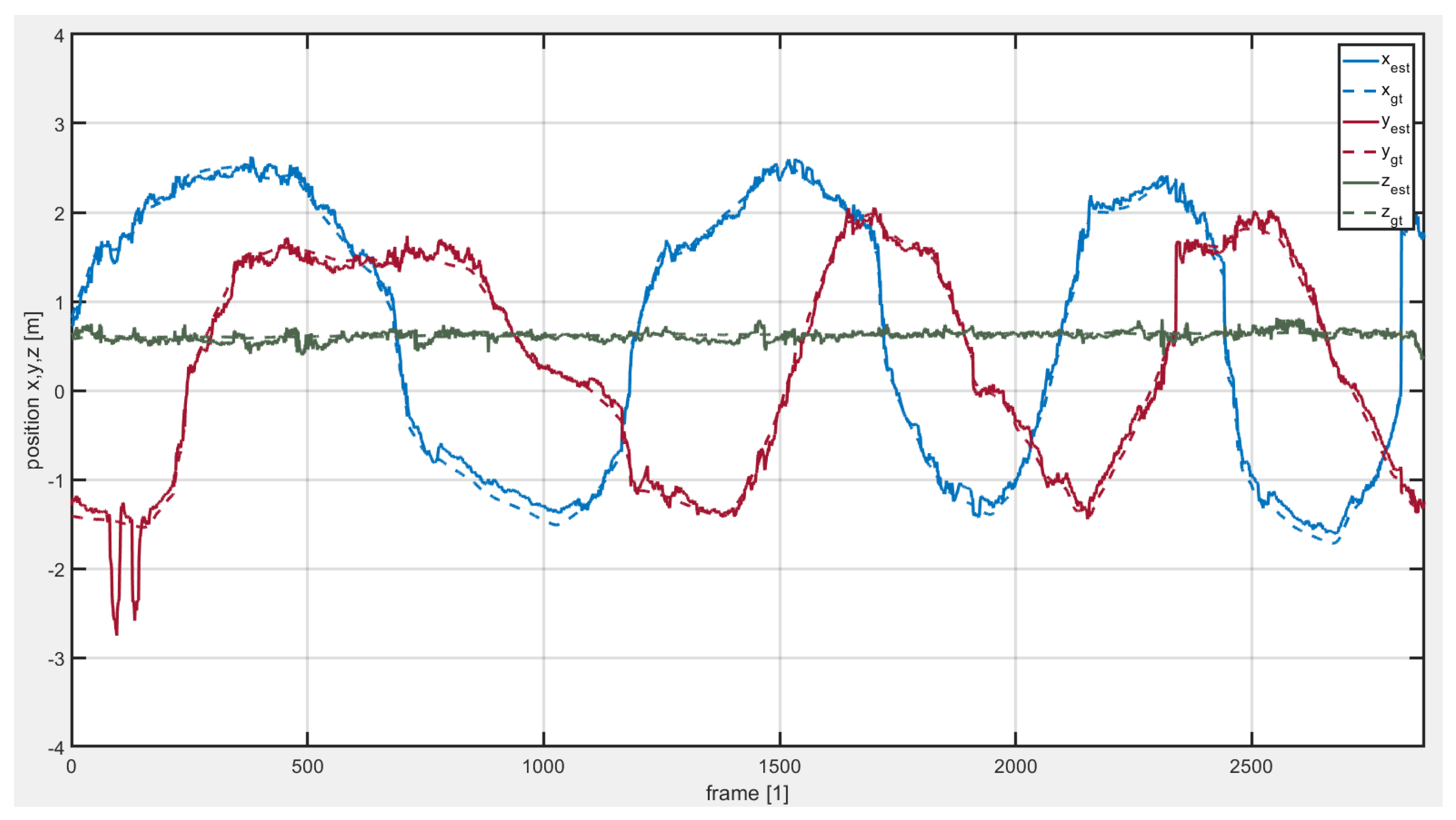
5.2. Indoor Experiment for 3D Position Estimation in VICON Environment

In the indoor experiment, our primary objective is to validate the effectiveness of the 3D tracking algorithm based on the Kalman filter. To achieve this, we conducted a controlled experiment where we temporarily removed the fixed setup of camera and LiDAR sensors from the UGV. Instead, we held the sensors setup in our hands and manually tracked the flying UAV within the VICON environment. The reason behind removing the sensors from the UGV is due to the limited size of the VICON environment, which is approximately seven by seven meters. This size constraint makes it challenging for the UGV to freely move around and track the UAV in real-time. The validity and credibility of VICON’s output results are paramount in shaping the evaluation of our positioning algorithm. By temporarily detaching the sensor setup from the UGV and holding it in our hands, we are liberated from spatial constraints, enabling us to gather ground truth data and algorithm output throughout the entire experiment. This approach allows us to conduct a comprehensive evaluation of the algorithm’s performance.
As demonstrated in Figure 2, the camera remains fixed above the LiDAR using a frame, ensuring that their relative positions are consistently maintained. The process of external parameter calibration is designed to determine the fixed external parameter matrix between these sensors, whether they are mounted on the UGV or held by hand. It is worth noting that over time, sensor positions may undergo changes due to factors like collisions, vibrations, or other external influences. This opens the door to a distinct avenue of research, automatic sensor calibration, a topic that may well be part of our future work. However, for the scope of this paper, we assume that the coordinate transformation matrix between sensors remains constant, owing to their fixed nature within their components.
To maintain data consistency and reliability, we adopted a specific approach in data collection. We chose to gather test data starting at 30 s after the sensors were initialized. This strategy ensured that we consistently acquired frames from different sensors with the same timestamp, which is crucial for the accurate initialization of the algorithm. It is worth emphasizing that the data collection process required the continuous and uninterrupted operation of the sensors within a designated time frame to reflect normal operating conditions. On rare occasions, unforeseen hardware issues could cause one or more sensors to disconnect suddenly from the computer. In such instances, data collected during these periods would be deemed invalid and excluded from the analysis to preserve the integrity of the dataset.
During the experiment, human operators took control of the UAV’s movements within the VICON environment. They executed various flight patterns and behaviors, including drawing circles, ascending, descending, and other maneuvers that simulate real-world scenarios and tasks. These movements allow us to assess the tracking algorithm’s performance in different situations and evaluate its ability to accurately estimate and track the 3D position of the UAV relative to the UGV. The ground truth was captured by VICON because it provides highly accurate and precise measurements of object movements, capturing the positions and orientations of objects with great detail. Figure 12 shows the visualization of algorithm-running process in the indoor experiment. To highlight the necessity of sensors fusion, we implemented the tracking algorithm with only stereo cameras for comparison. The performance is shown in Figure 13. The comparison between the ground truth positions and the estimated positions obtained from the stereo-camera-only algorithm highlighted the inconsistencies and larger deviations without sensors fusion.
We computed the error in the x, y, and z directions of the UAV’s position estimation. These errors were then visualized in Figure 14 and Figure 15, providing quantitative insights into the system’s accuracy, which was obtained by running different algorithm on the same dataset. By examining the distribution and magnitude of the errors, we gained a comprehensive understanding of the system’s performance in terms of position estimation. The mean value of the error is basically in the range of −0.3 m to 0.3 m. In the first 200 frames, due to the uncertainty of the pilot’s operation, the UAV accelerated in the y direction, which affected the accuracy of the information collected by the sensors. As seen, the errors were relatively large, but the errors were corrected within a short period of time, which verified the robustness of the proposed algorithm. The medians of the errors in the three directions are 0.061 m, 0.028 m, and 0.013 m, respectively, which is acceptable for the proposed system. And the RMSE is 0.032 m, which is smaller than that in [12,35].
To provide a visual representation of the results, we compared the ground truth position with the estimated position, as shown in Figure 16, which was obtained by running different algorithms on the same dataset. This allowed us to qualitatively assess the system’s ability to track and follow the UAV’s movements. By visually examining the alignment between the ground truth and estimated positions, we could evaluate the system’s precision and robustness.
Furthermore, we generated a 3D path using MATLAB, as shown in Figure 17, incorporating both the ground truth data and the estimated position. This path provided a comprehensive trajectory visualization, enabling us to analyze the overall performance of the system in tracking the UAV’s movements within the indoor environment.

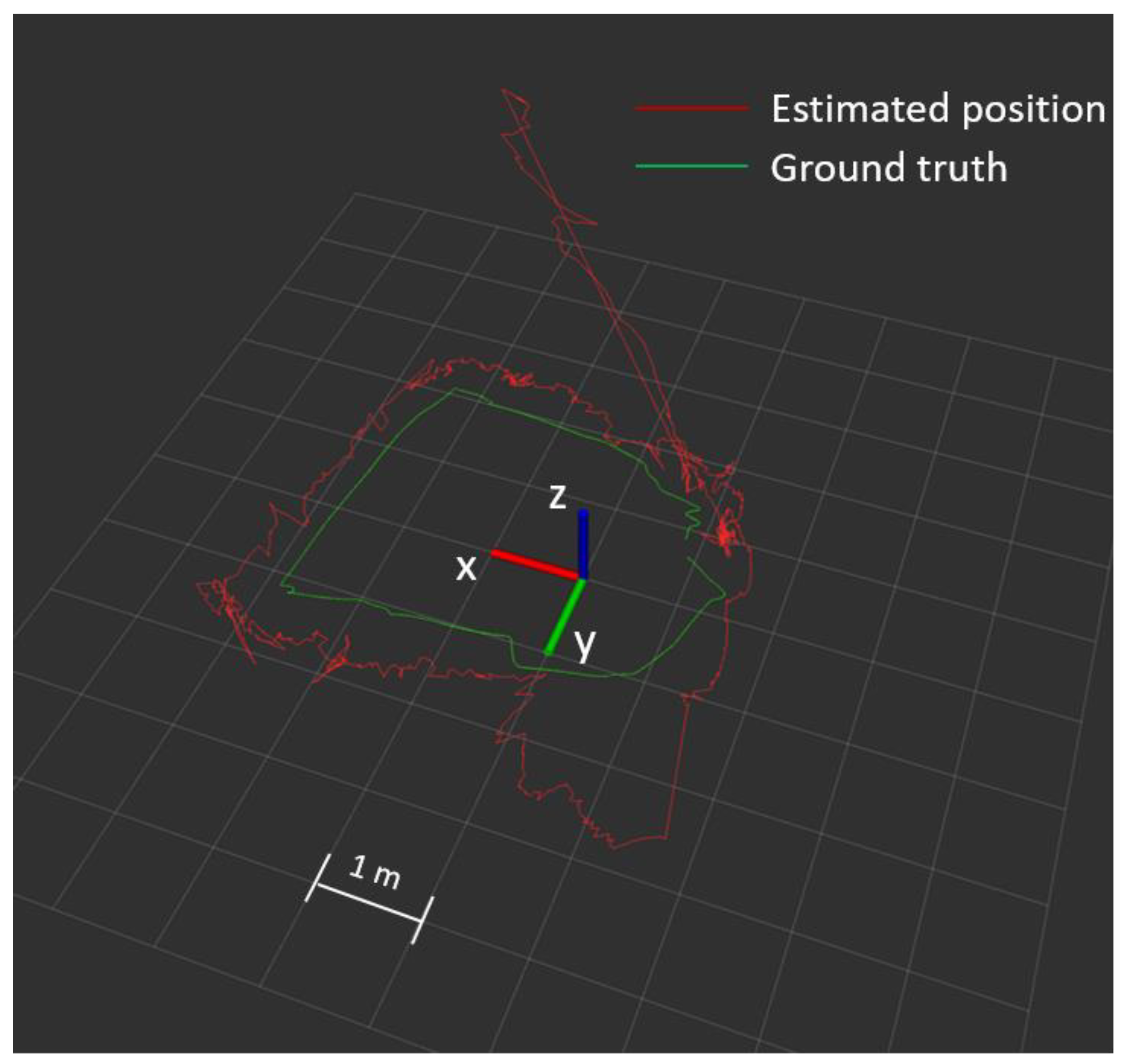
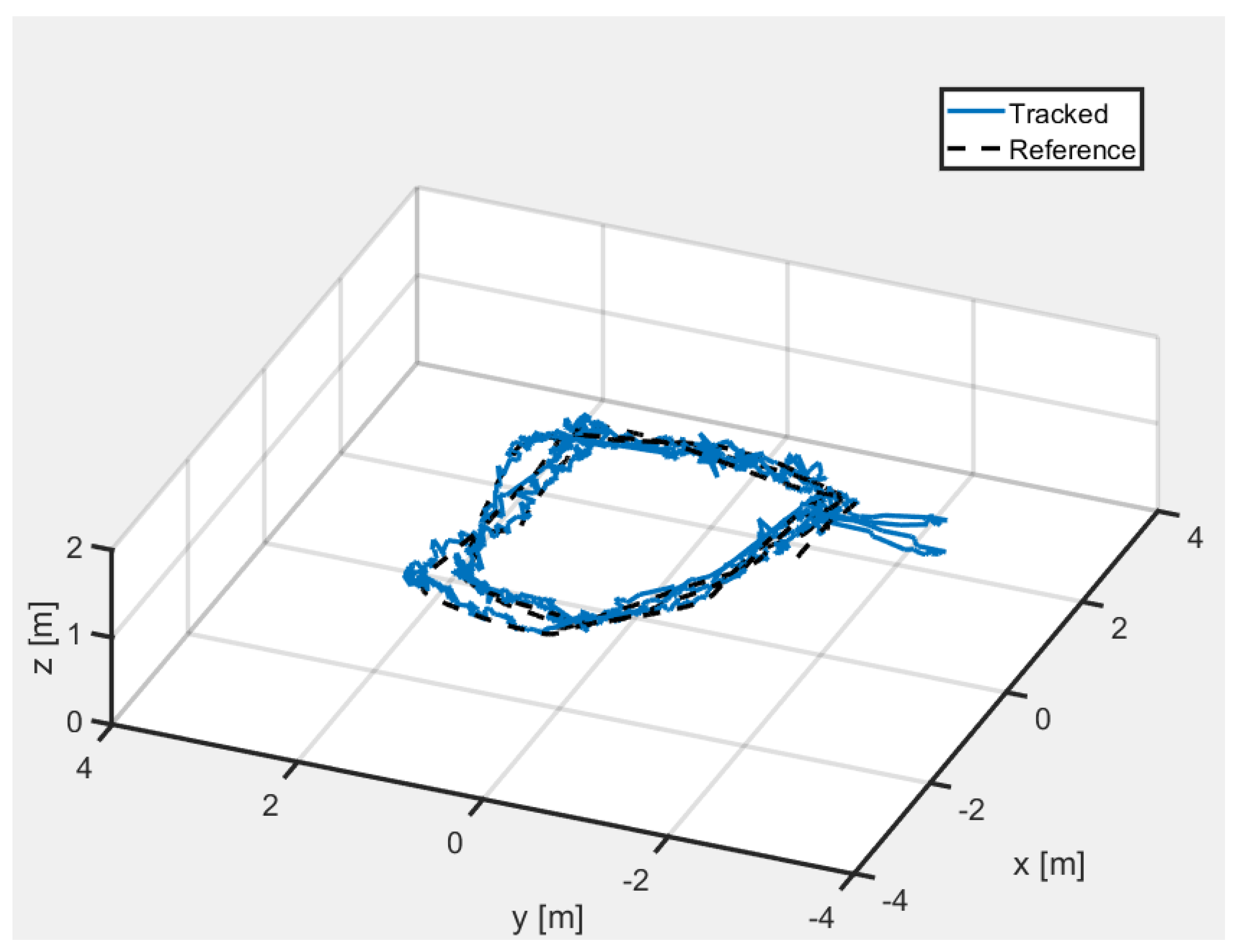
5.3. Filed Test in Outdoor Environment with LiDAR-Inertial Odometry (LIO)

In our outdoor experiment, our primary objective was to assess the efficacy of the proposed system in genuine real-world scenarios in which no ground truth reference was accessible for comparative analysis. This outdoor experiment encompassed the full scope of the automatic detection and tracking of UAVs by the UGV, equipped with the sensor setup. It effectively compensated for the limitation we encountered during indoor experiments in the VICON space, where it was not feasible to install the sensors directly on the UGV. In contrast to the indoor experiment where VICON was used for localization, we utilized an open ego-localization framework called FAST-LIO [36] from the MARS Laboratory of the University of Hong Kong, known for its high precision and efficiency in self-localization when providing accurate position information for the UGV in the outdoor environment. Notably, instead of a quantitative analysis, we focused on providing a visual assessment of the system’s performance.
During the outdoor experiment, the UAV, in this case, the F330 model, was manually controlled by a human operator. The purpose of manual control is to simulate realistic scenarios and behaviors that may occur during UAV operations in outdoor environments. The human operator can execute various flight maneuvers and trajectories, testing the robustness and effectiveness of the proposed system under different conditions.
After the target object is detected, the 3D tracking algorithm outputs the real-time 3D positions of the object and generates the desired waypoints. The waypoints are then transformed into the world frame using a transformation matrix, with the origin of the world box being the UGV’s starting position at the beginning of the algorithm. This transformation matrix is output in real time by the LIO frame and represents the current position of the UGV in the world frame.
Subsequently, the waypoints and the positions of the UGV are passed through a PID controller to generate a driving twist, which is sent to the UGV driver to control the movement of the UGV. The positions of both the UAV and the UGV in the world frame are plotted in Rviz for visualization and evaluation purposes, as shown in Figure 18. The red line is for the UGV’s position, and the green one is for the UAV’s.

5.4. Limitation Study

The use of a simple PID controller for UGV control introduces limitations to the tracking performance of the system. The PID controller is a classic control algorithm that operates based on error feedback and adjusts control signals accordingly. While PID controllers are widely used and effective in many applications, they have certain limitations.
One limitation is the response time of the PID controller, which may restrict the UGV’s ability to track the UAV accurately during high-speed movements. The controller’s response may not be fast enough to compensate for rapid changes in the UAV’s position, resulting in tracking errors or delays. Experiments show that the speeds of the UAV and UGV are affected by the above-mentioned condition, and that the tracking effect is the best when the UAV/UGV speed is around 1 m/s.
Additionally, the simplicity of the PID controller may limit its ability to handle complex maneuvers or trajectories. The control algorithm assumes a linear relationship between the error and the control signal, which may not capture the full dynamics of the UGV-UAV system during fast or agile movements. This can impact the system’s ability to accurately track the UAV’s position and trajectory. To overcome this, Jiang et al.’s method [37] employs neural networks to achieve model predictive control, offering adaptability, improved performance in nonlinear systems, and the ability to predict future states and optimize control inputs over a finite horizon.
Furthermore, the effective tracking range between the UGV and UAV may be limited due to the control capabilities of the PID controller. If the UAV moves too far away from the UGV, the tracking performance may degrade as the UGV struggles to maintain accurate control over the UAV’s position. The best tracking distance is around 5–7 m.
Apart from the inherent limitations of the PID controller, it is essential to take into account the constraints associated with the field of view (FOV) of the sensor system. While the field of view (FOV) of the proposed sensor system has been expanded in comparison to a single-sensor RGB-D camera, it is important to acknowledge that in complex terrains such as forests and construction sites, autonomous UAV tracking using a UGV, while simultaneously avoiding obstacles, presents a notable challenge. This challenge arises due to the potential for the UAV to move beyond the FOV as the UGV follows its planned obstacle avoidance path. This limitation is further compounded by the fact that the sensors are fixed on the UGV. To address this challenge, Z. Liu et al. [38] have proposed an innovative solution. Their suggestion involves the installation of a two-degree-of-freedom gimbal on the UGV, upon which the sensors are mounted. This approach allows for independent rotation of the gimbal, ensuring that the UAV remains within the FOV throughout the UGV’s movement. By implementing this solution, a more robust and effective tracking capability can be achieved, particularly in dynamic and obstacle-laden environments.

6. Conclusions

In conclusion, this study presents a novel system designed to enhance the capabilities of UAV/UGV-coordinated heterogeneous systems. We have successfully integrated a multitude of sensors to enable the detection, localization, and precise positioning of target objects, all while facilitating autonomous UGV navigation without any prior knowledge requirements. Notably, our system showcases a significant departure from the traditional tight-coupling method, as it effectively decouples the RGB-D camera and LiDAR components, resulting in a remarkable reduction in computational demands while maintaining high accuracy standards. Furthermore, it is worth noting that our system operates seamlessly with only CPU power, making it an efficient solution for various applications. The experimental findings demonstrate the system’s ability to perform in environments where GPS is unavailable, and the proposed method yields a satisfactory level of estimation accuracy.

7. Future Work

In the context of future work, it is envisaged that the path planning module can be extended to achieve a more advanced level of trajectory optimization. This optimization will be accomplished by incorporating factors such as the estimation of the target’s motion state, both dynamic and static obstacle constraints, as well as accounting for the physical limitations of the UGV. The overarching goal is to minimize the likelihood of collisions during UGV tracking tasks and enhance the overall robustness of the system.

Supplementary Materials

The following are available online at https://youtu.be/9CCYqunSRGs (accessed on 29 July 2023), Video: A Low-cost Relative Positioning Method for UAV/UGV Heterogeneous System based on Visual-Lidar Fusion, https://github.com/HKPolyU-UAV/GTA (accessed on 20 May 2023), Source code.

Author Contributions

Conceptualization, H.L.; methodology, H.L. and C.-Y.W.; software, H.L.; validation, H.L.; investigation, H.L.; resources, H.L. and C.-Y.W.; data curation, H.L.; writing—original draft preparation, H.L.; writing—review and editing, C.-Y.W.; supervision, C.-Y.W. All authors have read and agreed to the published version of the manuscript.

Funding

This study was performed with the support of Research Centre for Unmanned Autonomous Systems, Department of Aeronautical and Aviation Engineering, The Hong Kong Polytechnic University, under project ID P0042699.

Data Availability Statement

Not applicable.

Conflicts of Interest

The authors declare no conflict of interest.

Abbreviations

The following abbreviations are used in this thesis:
FPSFrames Per Second
IOUIntersection over Union
ROIRegion of Interest
LiDARLight Detection and Ranging
GNSSGlobal Navigation Satellite System
GM-APDGeiger-Mode Avalanche Photodiode
DNNDeep Neural Network
RANSACRandom Sample Consensus
CPUCentral Processing Unit
mAPMean Average Precision
ROSRobot Operating System
RMSERoot Mean Square Error
UAVUnmanned Aerial Vehicles
UGVUnmanned Ground Vehicles
LIOLiDAR Inertial Odometry
DOFDegree of Freedom
PTPPrecision Time Protocol
GPSGlobal Positioning System
PPSPulse Per Second
FOVField of View
R-CNNRegion-based Convolutional Neural Network
2D-BBTwo-dimensional Bounding Box
YOLOYou Only Look Once algorithm.

References

  1. Pretto, A.; Aravecchia, S.; Burgard, W.; Chebrolu, N.; Dornhege, C.; Falck, T.; Fleckenstein, F.; Fontenla, A.; Imperoli, M.; Khanna, R.; et al. Building an Aerial–Ground Robotics System for Precision Farming: An Adaptable Solution. IEEE Robot. Autom. Mag. 2021, 28, 29–49. [Google Scholar] [CrossRef]
  2. Ni, J.; Wang, X.; Tang, M.; Cao, W.; Shi, P.; Yang, S.X. An improved real-time path planning method based on dragonfly algorithm for heterogeneous multi-robot system. IEEE Access 2020, 8, 140558–140568. [Google Scholar] [CrossRef]
  3. Krizmancic, M.; Arbanas, B.; Petrovic, T.; Petric, F.; Bogdan, S. Cooperative Aerial-Ground Multi-Robot System for Automated Construction Tasks. IEEE Robot. Autom. Lett. 2020, 5, 798–805. [Google Scholar] [CrossRef]
  4. Magid, E.; Pashkin, A.; Simakov, N.; Abbyasov, B.; Suthakorn, J.; Svinin, M.; Matsuno, F. Artificial Intelligence Based Framework for Robotic Search and Rescue Operations Conducted Jointly by International Teams. In Proceedings of the 14th International Conference on Electromechanics and Robotics “Zavalishin’s Readings” ER (ZR) 2019, Kursk, Russia, 17–20 April 2019; pp. 15–26. [Google Scholar]
  5. Stampa, M.; Jahn, U.; Fruhner, D.; Streckert, T.; Rohrig, C. Scenario and system concept for a firefighting UAV-UGV team. In Proceedings of the 2022 Sixth IEEE International Conference on Robotic Computing (IRC), Naples, Italy, 5–7 December 2022; pp. 253–256. [Google Scholar]
  6. Hu, Z.; Bai, Z.; Yang, Y.; Zheng, Z.; Bian, K.; Song, L. UAV Aided Aerial-Ground IoT for Air Quality Sensing in Smart City: Architecture, Technologies, and Implementation. IEEE Netw. 2019, 33, 14–22. [Google Scholar] [CrossRef]
  7. Hammer, M.; Borgmann, B.; Hebel, M.; Arens, M. UAV detection, tracking, and classification by sensor fusion of a 360 lidar system and an alignable classification sensor. In Proceedings of the Laser Radar Technology and Applications XXIV, Baltimore, MD, USA, 16–17 April 2019; pp. 99–108. [Google Scholar]
  8. Sier, H.; Yu, X.; Catalano, I.; Queralta, J.P.; Zou, Z.; Westerlund, T. UAV Tracking with Lidar as a Camera Sensor in GNSS-Denied Environments. In Proceedings of the 2023 International Conference on Localization and GNSS (ICL-GNSS), Castellon, Spain, 6–8 June 2023; pp. 1–7. [Google Scholar]
  9. Dogru, S.; Marques, L. Drone Detection Using Sparse Lidar Measurements. IEEE Robot. Autom. Lett. 2022, 7, 3062–3069. [Google Scholar] [CrossRef]
  10. Asvadi, A.; Girao, P.; Peixoto, P.; Nunes, U. 3D object tracking using RGB and LIDAR data. In Proceedings of the 2016 IEEE 19th International Conference on Intelligent Transportation Systems (ITSC), Rio de Janeiro, Brazil, 1–4 November 2016; pp. 1255–1260. [Google Scholar]
  11. Dieterle, T.; Particke, F.; Patino-Studencki, L.; Thielecke, J. Sensor data fusion of LIDAR with stereo RGB-D camera for object tracking. In Proceedings of the 2017 IEEE Sensors, Glasgow, UK, 29 October–1 November 2017; pp. 1–3. [Google Scholar]
  12. Lo, L.Y.; Yiu, C.H.; Tang, Y.; Yang, A.S.; Li, B.; Wen, C.Y. Dynamic Object Tracking on Autonomous UAV System for Surveillance Applications. Sensors 2021, 21, 7888. [Google Scholar] [CrossRef] [PubMed]
  13. Li, J.; Ye, D.H.; Kolsch, M.; Wachs, J.P.; Bouman, C.A. Fast and Robust UAV to UAV Detection and Tracking from Video. IEEE Trans. Emerg. Top. Comput. 2022, 10, 1519–1531. [Google Scholar] [CrossRef]
  14. Liu, L.; He, J.; Ren, K.; Xiao, Z.; Hou, Y. A LiDAR–Camera Fusion 3D Object Detection Algorithm. Information 2022, 13, 169. [Google Scholar] [CrossRef]
  15. An, P.; Liang, J.; Yu, K.; Fang, B.; Ma, J. Deep structural information fusion for 3D object detection on LiDAR–camera system. Comput. Vis. Image Underst. 2022, 214, 103295. [Google Scholar] [CrossRef]
  16. Faessler, M.; Mueggler, E.; Schwabe, K.; Scaramuzza, D. A monocular pose estimation system based on infrared leds. In Proceedings of the 2014 IEEE International Conference on Robotics and Automation (ICRA), Hong Kong, China, 31 May–7 June 2014; pp. 907–913. [Google Scholar]
  17. Censi, A.; Strubel, J.; Brandli, C.; Delbruck, T.; Scaramuzza, D. Low-latency localization by active LED markers tracking using a dynamic vision sensor. In Proceedings of the 2013 IEEE/RSJ International Conference on Intelligent Robots and Systems, Tokyo, Japan, 3–7 November 2013; pp. 891–898. [Google Scholar]
  18. Hartmann, B.; Link, N.; Trommer, G.F. Indoor 3D position estimation using low-cost inertial sensors and marker-based video-tracking. In Proceedings of the IEEE/ION Position, Location and Navigation Symposium, Indian Wells, CA, USA, 4–6 May 2010; pp. 319–326. [Google Scholar]
  19. Eberli, D.; Scaramuzza, D.; Weiss, S.; Siegwart, R. Vision Based Position Control for MAVs Using One Single Circular Landmark. J. Intell. Robot. Syst. 2010, 61, 495–512. [Google Scholar] [CrossRef]
  20. Chang, C.-W.; Lo, L.-Y.; Cheung, H.C.; Feng, Y.; Yang, A.-S.; Wen, C.-Y.; Zhou, W. Proactive guidance for accurate UAV landing on a dynamic platform: A visual–inertial approach. Sensors 2022, 22, 404. [Google Scholar] [CrossRef] [PubMed]
  21. Wang, J.; Choi, W.; Diaz, J.; Trott, C. The 3D Position Estimation and Tracking of a Surface Vehicle Using a Mono-Camera and Machine Learning. Electronics 2022, 11, 2141. [Google Scholar] [CrossRef]
  22. Chen, H.; Wen, C.Y.; Gao, F.; Lu, P. Flying in Dynamic Scenes with Multitarget Velocimetry and Perception-Enhanced Planning. IEEE Asme T Mech 2023. [Google Scholar] [CrossRef]
  23. Quentel, A. A Scanning LiDAR for Long Range Detection and Tracking of UAVs; Normandie Université: Caen, France, 2021. [Google Scholar]
  24. Qingqing, L.; Xianjia, Y.; Queralta, J.P.; Westerlund, T. Adaptive Lidar Scan Frame Integration: Tracking Known MAVs in 3D Point Clouds. In Proceedings of the 2021 20th International Conference on Advanced Robotics (ICAR), Ljubljana, Slovenia, 6–10 December 2021; pp. 1079–1086. [Google Scholar]
  25. Qi, H.; Feng, C.; Cao, Z.; Zhao, F.; Xiao, Y. P2b: Point-to-box network for 3d object tracking in point clouds. In Proceedings of the IEEE/CVF Conference on Computer Vision and Pattern Recognition, Seattle, WA, USA, 14–19 June 2020; pp. 6329–6338. [Google Scholar]
  26. Ding, Y.; Qu, Y.; Zhang, Q.; Tong, J.; Yang, X.; Sun, J. Research on UAV Detection Technology of Gm-APD Lidar Based on YOLO Model. In Proceedings of the 2021 IEEE International Conference on Unmanned Systems (ICUS), Beijing, China, 15–17 October 2021; pp. 105–109. [Google Scholar]
  27. Chen, S.; Feng, Y.; Wen, C.-Y.; Zou, Y.; Chen, W. Stereo Visual Inertial Pose Estimation Based on Feedforward and Feedbacks. IEEE/ASME Trans. Mechatron. 2023, 1–11. [Google Scholar] [CrossRef]
  28. Gao, X.-S.; Hou, X.-R.; Tang, J.; Cheng, H.-F. Complete solution classification for the perspective-three-point problem. IEEE Trans. Pattern Anal. Mach. Intell. 2003, 25, 930–943. [Google Scholar]
  29. Marquardt, D.W. An algorithm for least-squares estimation of nonlinear parameters. J. Soc. Ind. Appl. Math. 1963, 11, 431–441. [Google Scholar] [CrossRef]
  30. Bradski, G. The openCV library. Dr. Dobb’s J. Softw. Tools Prof. Program. 2000, 25, 120–123. [Google Scholar]
  31. Redmon, J.; Divvala, S.; Girshick, R.; Farhadi, A. You only look once: Unified, real-time object detection. In Proceedings of the IEEE Conference on Computer Vision and Pattern Recognition, Las Vegas, NV, USA, 27–30 June 2016; pp. 779–788. [Google Scholar]
  32. Bochkovskiy, A.; Wang, C.-Y.; Liao, H.-Y.M. Yolov4: Optimal speed and accuracy of object detection. arXiv 2020, arXiv:2004.10934. [Google Scholar]
  33. Redmon, J.; Farhadi, A. Yolov3: An incremental improvement. arXiv 2018, arXiv:1804.02767. [Google Scholar]
  34. Tzutalin, D. LabelImg. GitHub Repository. Available online: https://github.com/HumanSignal/labelImg (accessed on 5 October 2015).
  35. Feng, Y.; Tse, K.; Chen, S.; Wen, C.Y.; Li, B. Learning-Based Autonomous UAV System for Electrical and Mechanical (E&M) Device Inspection. Sensors 2021, 21, 1385. [Google Scholar] [CrossRef]
  36. Xu, W.; Zhang, F. FAST-LIO: A Fast, Robust LiDAR-Inertial Odometry Package by Tightly-Coupled Iterated Kalman Filter. IEEE Robot. Autom. Lett. 2021, 6, 3317–3324. [Google Scholar] [CrossRef]
  37. Jiang, B.; Li, B.; Zhou, W.; Lo, L.-Y.; Chen, C.-K.; Wen, C.-Y. Neural network based model predictive control for a quadrotor UAV. Aerospace 2022, 9, 460. [Google Scholar] [CrossRef]
  38. Liu, Z.; Zhang, F.; Hong, X. Low-Cost Retina-Like Robotic Lidars Based on Incommensurable Scanning. IEEE/ASME Trans. Mechatron. 2022, 27, 58–68. [Google Scholar] [CrossRef]
Figure 1. The proposed tracking system demo in outdoor experiment.
Aerospace 10 00924 g001
Figure 2. The hardware platform for the UGV.
Aerospace 10 00924 g002
Figure 3. The F330 UAV set up.
Aerospace 10 00924 g003
Figure 4. The software architecture of the UGV’s automatic UAV tracking system.
Aerospace 10 00924 g004
Figure 5. The planar board data from the RGB camera and the LiDAR camera for calibration from different angles and distances. The RGB image above and the point cloud image below were collected by the RGB camera and LiDAR at the same time and correspond one to one. Four corresponding corner pairs within the two images are manually extracted.
Aerospace 10 00924 g005
Figure 6. The frame of PnP problem.
Aerospace 10 00924 g006
Figure 7. 2D bounding box (yellow rectangle) on the image plane predicted by YOLOv4-tiny with relative coordinates.
Aerospace 10 00924 g007
Figure 8. Image samples of the custom dataset. Images of the yellow ball and the UAV from different angles, scenes, distances, and clarity were collected to train the yolo model.
Aerospace 10 00924 g008
Figure 9. The ROI (green) for depth extraction after applying a scale factor on 2D bounding box from YOLOv4-tiny.
Aerospace 10 00924 g009
Figure 10. The workflow of the tracking algorithm.
Aerospace 10 00924 g010
Figure 11. The workflow of the Kalman filter.
Aerospace 10 00924 g011
Figure 12. Rviz visualization interface of algorithm running process with sensors fusion. The green line indicates the ground truth position, and the red line represents the estimated position. The side length of each square grid is 1 m.
Aerospace 10 00924 g012
Figure 13. Rviz visualization interface of algorithm running process with the stereo camera only. The green line indicates the ground truth position, and the red line represents the estimated position. The side length of each square grid is 1 m.
Aerospace 10 00924 g013
Figure 14. Position errors of x, y, and z directions in indoor experiment.
Aerospace 10 00924 g014
Figure 15. Boxplot of position errors in x, y, and z directions in indoor experiment.
Aerospace 10 00924 g015
Figure 16. Comparison of ground true position and estimated position in indoor experiment.
Aerospace 10 00924 g016
Figure 17. 3D path incorporating both the ground truth data and the estimated position in the indoor experiment.
Aerospace 10 00924 g017
Figure 18. Estimated position in world frame of the UGV and UAV (red line for UGV, and green line for UAV) and camera input from the view of UGV in outdoor experiment. Supplementary Materials: https://youtu.be/9CCYqunSRGs (accessed on 29 July 2023).
Aerospace 10 00924 g018
Table 1. Accuracy of YOLOv4-Tiny with respect to different resolutions based on CSPDarknet-53-tiny.
MethodBackboneResolutions A P 50
YOLOv4-TinyCSPDarknet-53-tiny320 × 32094.17%
416 × 41697.52%
512 × 51298.28%
608 × 60898.63%
Table 2. Speed (FPS) of YOLOv4-Tiny with respect to different resolutions based on different backbones (CSPDarknet-53-tiny and NCNN).
MethodResolutionsFPS (CSPDarknet-53-Tiny)FPS (NCNN)
YOLOv4-Tiny320 × 3202230
416 × 4162026
512 × 5121721
608 × 6081217
Table 3. Results of YOLOv4-Tiny trained with/without background images.
MethodBackboneResolutions A P 50
(Without Background Trained)
A P 50
(With Background Trained)
YOLOv4-TinyCSPDarknet-53-tiny320 × 32092.17%96.22%
416 × 41695.52%98.67%
512 × 51296.28%98.55%
608 × 60896.63%98.89%
Disclaimer/Publisher’s Note: The statements, opinions and data contained in all publications are solely those of the individual author(s) and contributor(s) and not of MDPI and/or the editor(s). MDPI and/or the editor(s) disclaim responsibility for any injury to people or property resulting from any ideas, methods, instructions or products referred to in the content.

