Receptivity and Stability Theory Analysis of a Transonic Swept Wing Experiment

Abstract

Surface suction provides an efficient way to delay boundary layer transitions. In order to verify the suction effects and determine the mechanism of suction control in transonic swept wing boundary layers, wind tunnel transition measurements in a hybrid laminar flow control (HLFC) wind tunnel model uses an infrared thermography technique in the Aircraft Research Association (ARA) 2.74 m × 2.44 m low turbulence level transonic wind tunnel. Based on the experimental data of stationary crossflow dominant transitions without and with surface suction in transonic swept wing boundary layers, in this paper, the effects on the receptivity and linear and nonlinear evolution of stationary crossflow vortices have been analyzed with the consideration of curvature. Theoretical analysis agreed with the experimental observations in regard to the transition delay caused by boundary layer suction near the leading-edge region.

1. Introduction

Laminar flow technology plays a very important role in aerodynamic drag reduction research, which is a development target in green aviation [1]. Generally, laminar techniques include natural laminar flow design and laminar flow control (suction, discrete roughness, dielectric barrier discharge plasma, wall cooling, etc.). These techniques have been proven to be very meaningful, effective and practicable in many works [2,3,4,5,6].

In this laminar technique, suction operations are focused on because of their significant effect on transition control, which has been confirmed and verified in wind experiments [7]. In order to study how suction operations affect the boundary layer, researchers have carried out a large amount of experimental research which, besides also targeting other areas, has mainly focused on suction control effects on turbulent separation, aerodynamic lift and drag and stall.

In recent years, several experimental studies have concentrated on the suction effects on boundary layer instability and their significance in the transition process. Saric [7] conducted research on the effects of suction and blowing on the flat plate boundary layer and documented the stabilizing effects of suction for Tollmien–Schlichting (TS) waves, which may delay the transition. The research of Arnal et al. [8], Bippes [9] and Shi et al. [10,11,12] demonstrates the significant effect of suction control on swept wings, swept flat plates and airfoils. The Langley Research Center has designed a swept supercritical airfoil incorporating laminar flow control (LFC) for testing at transonic speeds [13], but they did not analyze the details of boundary layer instability waves. Schülein [14] measured the suction control phenomena on a supersonic swept wing at the DLR Göttingen Ludwieg Tube Facility and pointed out that suction leads to the expected delay of transitions in the swept wing in wind tunnel tests. Regrettably, these experiments did not reveal the detailed mechanism of suction effects on crossflow instability-dominated transitions.

To determine the theoretical mechanism, researchers have conducted plenty of numerical simulations. They have found that streamwise and crossflow instabilities dominate most transition processes in the airfoil boundary layer. In addition, the suction upstream also has a transition delaying effect. For streamwise instability, Tilton and Cortelezzi [15] conducted a spatial linear stability analysis of the asymptotic suction boundary layer and found that small amounts of wall permeability may destabilize the Tollmien–Schlichting wave. Balakumar [16] conducted DNS simulations of a supersonic flat plate, which showed that the boundary layer is completely stabilized over the suction region. The boundary layer starts to become unstable downstream of the suction. However, the growth rates remain lower than those without suction for a long distance downstream. This implies that the transition occurs further downstream or does not occur at all in the entire region of the supersonic flat plate. For crosswise instability, Mack [17] simulated the linear stability of a suction boundary layer and found the maximum amplification rate varies almost linearly with the suction magnitude. Moreover, the stationary crossflow instability is sensitive to the locations of suction near the leading edge, but the Tollmien–Schlichting instability is not. Researchers [18,19,20,21] found that suction can change the initial amplitude of crossflow unstable waves compared to flow without suction. Kloker et al. [22,23] proved that micron-sized suction can stabilize the crossflow waves, and they used the Upstream Flow Deformation (UFD) technique combined with suction to analyze the effects on the crossflow instability in Falkner–Skan–Cooke velocity profiles and summarized the excitation of subharmonic spanwise modes. They indicated that if an appropriate design hole spacing is introduced, a suitable spanwise disturbance will reduce the amount of suction. Xu et al. [24] carried out a secondary instability analysis of stationary crossflows modified by suction in theoretical transonic swept wing boundary layers and pointed out that suction on the wall can effectively weaken the crossflow development and secondary instability under the assumed conditions.

However, few research works have paid close attention to the suction effects on the initial amplitude of dominant unstable waves in real transonic swept wings compared to experimental data. According to Saric’s experimental and theoretical research [25,26,27,28,29], stationary crossflow waves, that is, when the wave frequency is equal to zero, usually dominate the crossflow instabilities in low turbulence disturbance environments. So, here, the stationary crossflow instabilities are only focused on due to their common role in aeronautical flow transitions. In the following sections, based on the experimental data of stationary crossflow dominant transitions without and with surface suction in transonic swept wing boundary layers, the effects of stationary crossflow vortices on the receptivity and linear and nonlinear evolution will be analyzed. We will try to present a relatively clear explanation of the stability mechanism of significant crossflow transition delays due to surface suction near the leading edge region.

2. Experimental Setup

The HLFC wind tunnel model was designed by the Aircraft Research Association (ARA) and Northwestern Polytechnical University (NPU), as shown in Figure 1, and experiments were conducted under various flow conditions. The wind tunnel model is a combination of an infinite swept wing with a 35 deg swept angle and fuselage; hence, the test region in the middle of the wing can be considered as an infinite swept wing configuration. Therefore, a theoretical analysis was performed using the infinite swept wing assumption. The details of this transonic swept wing design, wind tunnel experiment setup and the porous surface near the leading edge are fully described in [30,31]. It should be acknowledged that the crossflow instabilities dominate the transition at an angle of attack of −3.06 deg., Mach number of 0.7, and Reynolds number of 6.5 million based on the chord length c = 0.52615 m. The wind tunnel freestream turbulence intensity level is as low as 0.1%, resulting in stationary crossflow waves dominating the transition process. In addition, the suction holes are designed for the evenly distributed suction in order to obtain a steady surface suction effect. They have an average diameter with 51 μm, and the suction porous skin is distributed from the leading edge to a 20.0%c position with a hole spacing of 0.54 mm. The surface roughness height is about 0.3 μm and the porous surface area is about 0.04 m². In this study, the suction mass rates (MRs) are 2.78 g/s and 3.36 g/s in the experiments, respectively. All the experimental data are measured by infrared thermography, and the way of suction is steady. It should be noted that the tunnel floor does not affect the experimental results in the middle wing.

Thermal convection in the turbulent boundary layer is stronger than that in laminar flow, resulting in a distinct wall temperature difference between the laminar flow region and the turbulent flow region. Based on this characteristic, thermal measurement technology can be used for the identification of transition regions. For example, in Figure 2, the color of the laminar flow region is different from that of the turbulent flow region, and the jagged transition region is a typical phenomenon of stationary crossflow instability. Herein, the surface temperature is measured by the infrared (IR) thermography. Figure 2 displays the IR image of the upper surface of the HFLC wind tunnel model at the condition mentioned above, including the measurements with suction mass rates of 2.78 g/s and 3.36 g/s in Figure 2. The suction control cases in Figure 2b are labeled as ‘Case 1’ and ‘Case 2’, respectively. It can be observed in the figure that the natural crossflow dominated transition with a jagged shape on the outboard wing occurs near the 13.5% c position, the crossflow instability with a suction mass rate of 2.78 g/s appears about the 35.7% c position and the crossflow induced transition with suction mass rate of 3.36 g/s takes place close to the 48% c position. Note that the experimental setup can provide a stable suction flowrate; thus, a steady flowrate for the following numerical analysis can be safely assumed. Based on these measured data, we would perform our analysis and try to find the mechanism of suction effects.

3. Mathematical Methods

The boundary layer equations of infinite swept wing, compressible linear stability theory equations, compressible parabolic stability equations and bi-global instability equations are solved for the present theoretical analysis. Because of the maturation of these methods, a brief description for them is given in the following.

3.1. Boundary Layer Equations

The governing equations for compressible infinite swept wing boundary layers are given by

$$\begin{array}{c}\frac{\mathsf{\partial }}{\mathsf{\partial }{x}^{*}}\left({\rho }^{*}{U}^{*}\right)+\frac{\mathsf{\partial }}{\mathsf{\partial }{y}^{*}}\left({\rho }^{*}{V}^{*}\right)=0\\ {\rho }^{*}{U}^{*}\frac{\mathsf{\partial }{U}^{*}}{\mathsf{\partial }{x}^{*}}+{\rho }^{*}{V}^{*}\frac{\mathsf{\partial }{U}^{*}}{\mathsf{\partial }{y}^{*}}=-\frac{\mathsf{\partial }{p}^{*}}{\mathsf{\partial }{x}^{*}}+\frac{\mathsf{\partial }}{\mathsf{\partial }{y}^{*}}\left({\mu }^{*}\frac{\mathsf{\partial }{U}^{*}}{\mathsf{\partial }{y}^{*}}\right)\\ {\rho }^{*}{U}^{*}\frac{\mathsf{\partial }{W}^{*}}{\mathsf{\partial }{x}^{*}}+{\rho }^{*}{V}^{*}\frac{\mathsf{\partial }{W}^{*}}{\mathsf{\partial }{y}^{*}}=\frac{\mathsf{\partial }}{\mathsf{\partial }{y}^{*}}\left({\mu }^{*}\frac{\mathsf{\partial }{W}^{*}}{\mathsf{\partial }{y}^{*}}\right)\\ {\rho }^{*}{U}^{*}{c}_p^{*}\frac{\mathsf{\partial }{T}^{*}}{\mathsf{\partial }{x}^{*}}+{\rho }^{*}{V}^{*}{c}_p^{*}\frac{\mathsf{\partial }{T}^{*}}{\mathsf{\partial }{y}^{*}}=\frac{\mathsf{\partial }}{\mathsf{\partial }{y}^{*}}\left(\frac{{\mu }^{*}}{\mathrm{Pr}}\frac{\mathsf{\partial }{W}^{*}}{\mathsf{\partial }{y}^{*}}\right)+U^{*}\frac{\mathsf{\partial }{p}^{*}}{\mathsf{\partial }{x}^{*}}+{\mu }^{*}\left[{\left(\frac{\mathsf{\partial }{U}^{*}}{\mathsf{\partial }{y}^{*}}\right)}^2+{\left(\frac{\mathsf{\partial }{W}^{*}}{\mathsf{\partial }{y}^{*}}\right)}^2\right]\end{array}$$

(1)

subject to the boundary conditions

$$\begin{array}{l}{y}^{*}=0,U^{*}=W^{*}=0,V^{*}=V_w^{*},\mathsf{\partial }{T}^{*}/\mathsf{\partial }{y}^{*}=0;\\ y^{*}={\delta }^{*},U^{*}=U_e^{*},W^{*}=W_e^{*},T^{*}=T_e^{*}.\end{array}$$

(2)

where x* is the arc length from the attachment line in the direction perpendicular to the leading edge, y* is the wall-normal coordinate, z* is the spanwise coordinate parallel to the leading edge (not present in Equations (1) and (2), but it appears later on). Corresponding to the defined system, U*, V*, and W* stand for the chordwise, wall-normal and spanwise velocities, respectively. In addition, ρ*, T*, p*, μ*, δ*, $c_p^{*}$ and Pr stand for the density, temperature, pressure, molecular viscosity, boundary layer thickness, specific heat at constant pressure and Prandt number, respectively. $V_w^{*}$ is the wall normal velocity, which is equal to zero without the suction.

At least 100 grid points are arranged in the boundary layer to solve the boundary layer equations, which is carried out by a unilateral second-order difference along the flow direction and spectral method along the wall-normal direction. The Chebyshev–Gauss–Lobatto function serves as the configuration point for the spectral method. The details can be found in [32,33].

3.2. Perturbation Equations

Any instantaneous variables are equal to the sum of perturbation variables ${\varphi }^{\prime }=\left[{\rho }^{\prime },u^{\prime },v^{\prime },w^{\prime },T^{\prime }\right]$ and mean flow ones. Substituting the sum form into the Navier–Stokes equations and subtracting the governing equations of mean flow, the compact scheme of perturbation equations is obtained as follows:

$$\begin{array}{l}(\Gamma \frac{\mathsf{\partial }}{\mathsf{\partial }t}+A\frac{\mathsf{\partial }}{\mathsf{\partial }x}+B\frac{\mathsf{\partial }}{\mathsf{\partial }y}+C\frac{\mathsf{\partial }}{\mathsf{\partial }z}+D+V_{xx}\frac{{\mathsf{\partial }}^2}{\mathsf{\partial }{x}^2}+V_{yy}\frac{{\mathsf{\partial }}^2}{\mathsf{\partial }{y}^2}\\ +V_{zz}\frac{{\mathsf{\partial }}^2}{\mathsf{\partial }{z}^2}+V_{xy}\frac{{\mathsf{\partial }}^2}{\mathsf{\partial }x\mathsf{\partial }y}+V_{yz}\frac{{\mathsf{\partial }}^2}{\mathsf{\partial }y\mathsf{\partial }z}+V_{xz}\frac{{\mathsf{\partial }}^2}{\mathsf{\partial }x\mathsf{\partial }z}){\varphi }^{\prime }=F_n\end{array}$$

(3)

where the coefficient matrixes $\Gamma ,A,B,C,D,V_{xx},V_{yy},V_{zz},V_{xy},V_{yz},V_{xz}$ and nonlinear term $F_n$ with curvature can be derived as shown in Chang’s paper [34].

3.3. Linear Stability Theory (LST)

The disturbance in LST analysis has the form

$${{\varphi }^{\prime }}_{LST}(x,y,z,t)=\widehat{\varphi }(y)e^{\mathrm{i}(\alpha x+\beta z-\omega t)}+c.c.$$

(4)

where $\widehat{\varphi }(y)$ represents the disturbance shape function for each disturbance variable, $\alpha ,\beta ,\omega$ indicate the complex wave number in the chordwise direction, the wave number in the spanwise direction and frequency, respectively. Generally, in the spatial problem, ω and β are often real and α is complex. The real part of $\alpha$ denotes the wave number and the imaginary part means the growth rate. The form Equation (4) implies that the disturbances have very significant variations in the spatial and temporal region compared to the base flow. As a result, the parallel flow assumption can be introduced. With this assumption and the linearization, retaining the derivatives in the wall normal direction and removing the nonlinear terms in Equation (3), linear stability theory equations can be obtained which govern the dispersion relation of the disturbances in the flow. It is an eigenvalue problem, and there are many methods to solve it. The amplification factor N_CF,0 is defined as $N_{CF,0}=-{\displaystyle \underset{s_0}{\overset{s}{\int }}{\alpha }_{i}ds}$. The related e^N method has been developed to maturity [35,36,37,38,39,40,41].

3.4. Parabolized Stability Equations (PSE)

The LST can give a rough analysis on the instability. However, the cross-instability problem in the airfoil boundary layer is more complex. Two factors must be considered. One is the non-parallel effect. The crossflow mode can be unstable at the leading edge of the airfoil for the significant non-parallel characteristic of the boundary layer. As a result, the non-parallel flow has an amplified effect on the crossflow modes. The other one is the nonlinear effect. The cross-flow transition usually has a saturated process of the unstable mode, which comes from the nonlinear effect of the instability. Then, considering both the non-parallelism and the nonlinear effect, parabolic stability equations were adopted at present, which was proposed by Bertolotti [42,43] and developed by many researchers [44,45,46,47]. The disturbance variables in the nonlinear parabolized stability equation (NPSE) method have the form

$${{\varphi }^{\prime }}_{NPSE}(x,y,z,t)={\displaystyle \sum _{m=-M}^M{\displaystyle \sum _{n=-N}^N{\widehat{\varphi }}_{mn}}}(x,y)e^{i{\displaystyle \int {\alpha }_{mn}}(\overline{x}d\overline{x})}{e}^{i(n\beta z-m\omega t)}+c.c.$$

(5)

$$F_n(x,y,z,t)={\displaystyle \sum _{m=-M}^M{\displaystyle \sum _{n=-N}^N{\widehat{F}}_{mn}}}{e}^{i(n\beta z-m\omega t)}+c.c.$$

(6)

These forms imply that the shape functions of disturbances are slowly variable in the streamwise direction, which suggests the non-parallel effect of the instability. Substituting Equations (5) and (6) into Equation (3), a compact scheme of the NPSE can be obtained by eliminating the ellipticity

$$(A_{mn}\frac{\mathsf{\partial }}{\mathsf{\partial }x}+B_{mn}-V_{xx}\frac{{\mathsf{\partial }}^2}{\mathsf{\partial }{x}^2}-V_{xy}\frac{{\mathsf{\partial }}^2}{\mathsf{\partial }x\mathsf{\partial }y}){\widehat{{\varphi }^{\prime }}}_{mn}={\widehat{F}}_{mn}$$

(7)

where the detailed expression of matrixes $A_{mn},B_{mn},V_{xx},V_{xy}$ and ${\widehat{F}}_{mn}$ can be found in Chang’s paper [34]. Removing the nonlinear terms, the equations are called the linear parabolic stability equations (LPSEs), which describe the linear development of given disturbances. Our solver for the LPSE and NPSE has been established and developed since 2005, and the code validations can be found in [48,49,50]. It is not necessary to repeat the validation here. Note that the NPSE method is used to describe the nonlinear evolution of the primary mode disturbance, and the distribution of the harmonic disturbances and the results are the foundation for secondary instability.

3.5. Receptivity Model

Since the traveling modes excited through the scale-conversion mechanism are only dominant in high-level turbulence environments, only the forced receptivity of the stationary mode directly excited by the surface roughness is considered here. In addition, natural roughness is inherently random in space; it is difficult to obtain the true receptivity amplitude, so only locally parallel receptivity analysis is conduct to evaluate suction effects on receptivity. The receptivity coefficient is solved with the help of the biorthogonal eigenfunction system, whose solver has been validated [51].

The no-slip and isothermal boundary conditions are imposed on the surface of the roughness, and the inhomogeneous boundary conditions of LST equations can be obtained by applying the first-order Taylor expansion:

$$\tilde{u}=\tilde{H}\left(\alpha ,\beta \right){\left.\frac{\mathsf{\partial }U}{\mathsf{\partial }y}\right|}_w,\tilde{v}=0,\tilde{w}=\tilde{H}\left(\alpha ,\beta \right){\left.\frac{\mathsf{\partial }W}{\mathsf{\partial }y}\right|}_w,\tilde{T}=0$$

(8)

where $\tilde{H}\left(\alpha ,\beta \right)$ is the double Fourier transform of the dimensionless height distribution function of surface roughness. With the help of the orthogonality relation, we can find the receptivity coefficient as the residue value at the pole. It is customary to normalize the eigenfunction by the maximum amplitude chordwise velocity, and the crossflow mode excited by surface roughness can be expressed as following,

$${\varphi }^{\prime }\left(x,y,z,t\right)=K\tilde{H}\left(\alpha ,\beta \right)\tilde{\varphi }\left(y\right)e^{i\alpha x+i\beta z-i\omega t}+c.c.$$

(9)

where K is the complex receptivity coefficient which represents the efficiency of the localized receptivity process independent of details of the surface geometry.

4. Experimental Data and Theoretical Analysis

4.1. Pressure Coefficient and Boundary Layer Solutions

In order to conduct the stability analysis as accurately as possible, we employ the transition model for crossflow instabilities in the laminar-turbulent transition prediction framework [52,53,54] to simulate the boundary layer flow. According to the CFD results with transition model, the accurate pressure distribution and variables at the edge of boundary layers can be obtained. Then, the compressible boundary layer equations are employed to provide the laminar base flow of the infinite swept wing for subsequent stability analysis. Both cases of suction and no suction control were calculated using CFD together with boundary layer equations. Through the CFD analysis, the pressure coefficient and variables at the edge of boundary layers can be solved anywhere on the airfoil, not relying on the coarse pressure tap locations of the experiment. Figure 3 illustrates the comparison of pressure distribution between CFD results and experimental data, showing excellent agreement. The CFD results are simulated through the improved NASA structured grid CFL3D solver for the mean flow with the third-order accuracy in space and second-order accuracy in time. Then, 6 million cells are employed for the simulation so that the y⁺ is smaller than 1.0. In the figure, x_c means the chordwise coordinate and c_n stands for the chord length normal to the leading edge.

Herein, the favorable pressure gradient region on the upper surface at the present experimental condition is focused on. Using the computed pressure coefficient, compressible boundary layer equations are solved to obtain the more accurate laminar base flow.

The comparison of velocity profiles before and after suction at five positions (5% c_n, 10% c_n, 20% c_n, 30% c_n, 40% c_n) is shown in Figure 4. The direction of the arrow indicates the direction from the leading edge to the trailing edge. It can be seen that the suction makes the boundary layer thickness thinner and weakens the crossflow strength. About the data used in Figure 4, $U_{s0}=U\cos \phi +W\sin \phi$, $W_{s0}=-U\sin \phi +W\cos \phi$, $U_s=U_{s0}/U_{s0e}$ and $W_s=W_{s0}/U_{s0e}$, where $U_{s0e}$ is the value of velocity $U_{s0}$ at the edge of the boundary layer and $\phi =\arctan \left(W_e/U_e\right)$ represents the local sweep angle. The results presented in Figure 4 indicate that the alleviated crossflow may stabilize the instability modes.

4.2. The Suction Effects on Linear Stability Property of Crossflow Waves

Although the crossflow transition is usually dominated by the nonlinear effect which is advised in the past research [46], the linear stability analysis also can suggest the main characteristics of the transition process, since the linear amplified region is the longest one in the whole transition process. In this section, the standard linear stability analysis is carried out through LST and LPSE methods. Figure 5a,b illustrate the LST analysis results considering curvature before and after suction, respectively. Here, λ represents the spanwise wavelength of crossflow vortices. Even though the crossflow vortices with the wavelength of 1.694 mm have the maximum value of N_CF,0 factor, the crossflow vortices with the wavelength of 0.965 mm dominates the transition compared with the measured transition position of 13.5% c_n. After the suction with a mass rate of 3.36 g/s, the whole crossflow strength is weakened, but the relative dispersion relation has not changed. The crossflow vortices with the wavelength of 1.694 mm, which also has the maximum value of N_CF,0 factor, becomes the dominant unstable wave at this state.

With further analysis, the linear stability properties considering non-parallelism using the LPSE method also are performed. Figure 6a,b illustrate the LPSE analysis results considering non-parallelism before and after suction, respectively. It can be seen that the non-parallel effect raises the growth rate and amplification factor. It should be acknowledged that the foregoing analysis and selection of dominant waves using LST have been confirmed by the LPSE results in Figure 6, indicating that the relationships between different wavelengths do not change. In addition, it can be seen that the suction stabilizes the whole stationary crossflow vortices and changes the dominant one compared with the measured transition position. Note that there are small deviations between critical N factor of LPSE before and after suction compared with the measured data, as shown in Figure 7. Therefore, when studying the stability analysis of swept wing crossflow instability, assuming that the same critical N value is given, the transition position obtained by LST deviates greatly from the experimental results. Meanwhile, the transition position obtained by the LPSE method considers non-parallelism, and the position is consistent with the experimental results.

The saturation zone of crossflow vortices formed by nonlinear interactions is relatively long, and the LPSE method is linear and cannot analyze the nonlinear effects. Therefore, the NPSE is needed to analyze the nonlinear zone in the following.

4.3. Nonlinear Evolution of Crossflow Waves

Before performing nonlinear analysis, the initial amplitude needs to be known. We used the susceptibility analysis method in Section 3.4 to calculate the crossflow stationary vortices under uncontrolled and controlled states. The calculated receptivity coefficients of the crossflow vortices near the leading edge to the distributed rough elements are shown in Figure 8. It can be seen from the figure that under the effect of distributed roughness, the receptivity coefficients of the crossflow stationary vortices at different wavelengths in the suction state are slightly increased. But with the effect of distributed roughness increasing, if integrated along the flow direction, it will form a non-negligible amplitude correction. Therefore, when we perform NPSE calculations, we cannot simply consider the initial amplitudes to be the same. Instead, the initial amplitude after suction is twice that of the non-suction condition.

Figure 9a,b show the evolution of amplitude in Fourier modes where (0,0) is zero frequency and zero wave number, (0,1) is zero frequency and one times wave number of the fundamental dominant wave, (0,2) is two times wave number of the fundamental dominant wave, etc. In the expression, ‘0′ means zero frequency and the latter number from 1 to n indicates n times the wave number of the fundamental dominant wave. It can be seen that a significant transition delay is observed with suction, and the (0,1) fundamental mode always dominates, and there is only a short saturation region before the transition. The reason may be that the strong favorable pressure gradient and high Reynolds number in this case caused a rapid crossflow transition near the leading-edge region. According to the NPSE results in Figure 9 and Figure 10, the u-velocity contours computed from Equation (5) are sketched in the cross-sectional planes (z, y) at the saturated region under no control and control states. It can be seen that the crossflow vortices shape is fully developed in the saturation area, and the peak amplitude of the crossflow vortices in the saturation area is weakened due to the influence of surface suction, which is similar with the results in Refs. [24,25,46]. It should be noted that when post-processing the crossflow vortices contour of the NPSE results, in order to display the complete crossflow vortices, only about one times boundary layer thickness was taken in the wall-normal direction in the figure. The computational domain in the wall-normal direction of the NPSE is approximately 30 times the thickness of the boundary layer. This will affect the dominant mode characteristics of the secondary instability stage. In Figure 11, the integrated amplification factors of the primary (0,1) mode under no control and control states through the NPSE are displayed, indicating the nonlinear effect reduces the N factor.

5. Conclusions

Based on the HLFC wind tunnel experiment, we have carried out the related theoretical analysis before and after suction in the transonic swept-wing boundary layers. Our two main conclusions are outlined below:

(1)

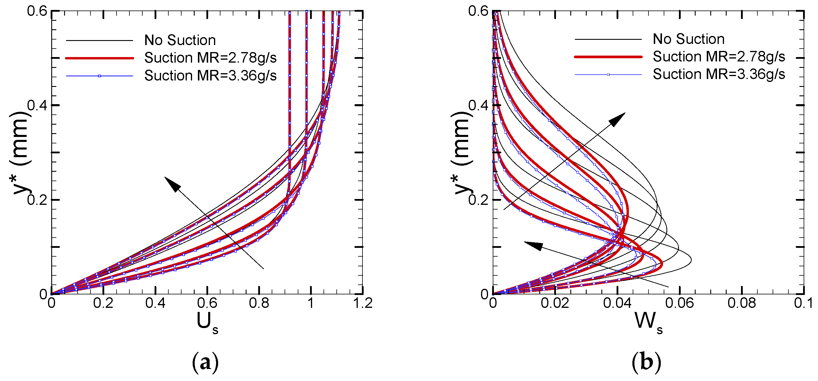
Both theory and experiments have proved that surface suction can delay the transition through changing the laminar base flow, and the most unstable crossflow vortices are suppressed. With the surface suction, the saturation region of the crossflow vortices is significantly delayed, and the peak amplitude of the saturated crossflow vortices is also weakened, which will affect the dominant mode characteristics of the secondary instability stage.

(2)

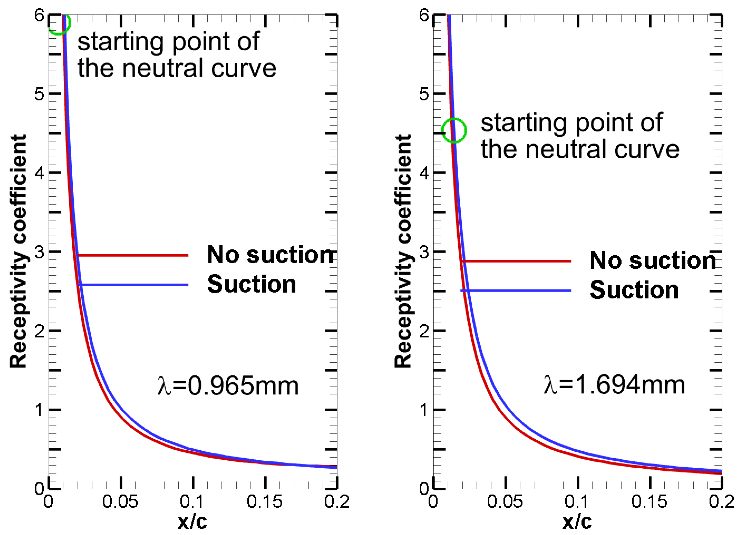
The LST and PSE methods are useful for stability analysis to obtain information about the most unstable waves, especially how the unstable waves evolve after taking into account curvature, non-parallel and nonlinear effects. The receptivity coefficients of the crossflow instability vortices to the distributed roughness will increase when the surface suction is activated. Therefore, the same initial amplitudes cannot be chosen for NPSE analysis.

References

1. Malik, M.R.; Crouch, J.D.; Saric, W.S.; Lin, J.C.; Whalen, E.A. Application of drag reduction techniques to transport aircraft. In Encyclopedia of Aerospace Engineering; John Wiley & Sons, Ltd.: Hoboken, NJ, USA, 2010; pp. 1–10. [Google Scholar]
2. Collier, F., Jr. An overview of recent subsonic laminar flow control flight experiments. In Proceedings of the 23rd Fluid Dynamics, Plasma dynamics, and Lasers Conference, Orlando, FL, USA, 6–9 July 1993; p. 2987. [Google Scholar]
3. Joslin, R.D. Overview of Laminar Flow Control, 1998, TP-1998-208705; NASA Langley Research Center: Hampton, VA, USA, 1998.
4. Joslin, R.D. Aircraft laminar flow control. Annu. Rev. Fluid Mech. 1998, 30, 1–29. [Google Scholar] [CrossRef]
5. Crouch, J.; Sutanto, M.; Witkowski, D.; Watkins, A.; Rivers, M.; Campbell, R. Assessment of the national transonic facility for natural laminar flow testing. In Proceedings of the 48th AIAA Aerospace Sciences Meeting including the New Horizons Forum and Aerospace Exposition, Orlando, FL, USA, 4–7 January 2010; p. 1302. [Google Scholar]
6. Crouch, J. Boundary-layer transition prediction for laminar flow control. In Proceedings of the 45th AIAA Fluid Dynamics Conference, Dallas, TX, USA, 22–26 June 2015; p. 2472. [Google Scholar]
7. Saric, W.; Reed, H. Effect of suction and blowing on boundary-layer transition. In Proceedings of the 21st Aerospace Sciences Meeting, Reno, NV, USA, 10–13 January 1983; p. 43. [Google Scholar]
8. Arnal, D.; Gasparian, G.; Salinas, H. Recent advances in theoretical methods for laminar turbulent transition prediction. In Proceedings of the 36th AIAA Aerospace Sciences Meeting and Exhibit AIAA Paper, Reno, NV, USA, 12–15 January 1998; p. 223. [Google Scholar]
9. Bippes, H. Basic experiments on transition in three-dimensional boundary layers dominated by crossflow instability. Prog. Aerosp. Sci. 1999, 35, 363–412. [Google Scholar] [CrossRef]
10. Shi, Y.; Bai, J.; Hua, J.; Yang, T. Numerical analysis and optimization of boundary layer suction on airfoils. Chin. J. Aeronaut. 2015, 28, 357–367. [Google Scholar] [CrossRef]
11. Shi, Y.; Yang, T.; Bai, J.; Lu, L.; Wang, H. Research of transition criterion for semi-empirical prediction method at specified transonic regime. Aerosp. Sci. Technol. 2019, 88, 95–109. [Google Scholar] [CrossRef]
12. Shi, Y.; Cao, T.; Yang, T.; Bai, J.; Qu, F.; Yang, Y. Estimation and analysis of hybrid laminar flow control on a transonic experiment. AIAA J. 2020, 58, 118–132. [Google Scholar] [CrossRef]
13. Brooks, C.W., Jr.; Harris, C.D.; Harvey, W.D. The NASA Langley Laminar-Flow-Control Experiment on a Swept, Supercritical Airfoil-Drag Equations; NASA: Hamton, VA, USA, 1989.
14. Schülein, E. Experimental investigation of laminar flow control on a supersonic swept wing by suction. In Proceedings of the 4th Flow Control Conference, Seattle, WA, USA, 23–26 June 2008; p. 4208. [Google Scholar]
15. Tilton, N.; Cortelezzi, L. Stability of boundary layers over porous walls with suction. AIAA J. 2015, 53, 2856–2868. [Google Scholar] [CrossRef]
16. Balakumar, P. Control of supersonic boundary layers using steady suction. In Proceedings of the 36th AIAA Fluid Dynamics Conference and Exhibit, Online, 5 June 2006. [Google Scholar]
17. Mack, L.M. Compressible boundary-layer stability calculations for sweptback wings with suction. AIAA J. 1982, 20, 363–369. [Google Scholar] [CrossRef]
18. Arnal, D.; Seraudie, A.; Archambaud, J.P. Influence of Surface Roughness and Suction on the Receptivity of a Swept Wing Boundary Layer. In Laminar–Turbulent Transition, Proceedings of the IUTAM Symposium, Sedona, AZ, USA, 13–17 September 1999; Fasel, H.F., Saric, W.S., Eds.; Springer: Berlin/Heidelberg, Germany, 1999. [Google Scholar]
19. Xu, J.; Wu, X. Surface-roughness effects on crossflow instability of swept-wing boundary layers through generalized resonance mechanisms. AIAA J. 2022, 60, 2887–2904. [Google Scholar] [CrossRef]
20. Abegg, C.; Bippes, H.; Bertolotti, F.P. On the application of suction for the stabilization of crossflow instability over perforated walls. In New Results in Numerical and Experimental Fluid Dynamics, Proceedings of the 11th AG STAB/DGLR Symposium, Notes on Numerical Fluid Mechanics, 16–18 January 1987, Kiel, Germany; Nitsche, W.G., Heinemann, H.-J., Hilbig, R., Eds.; Vieweg: Wiesbaden, Germany, 1999; Volume 72. [Google Scholar]
21. Abegg, C.; Bippes, H.; Janke, E. Stabilization of Boundary-Layer Flows Subject to Crossflow Instability with the Aid of Suction. In Laminar–Turbulent Transition, Proceedings of the IUTAM Symposium, Sedona, AZ, USA, 13–17 September 1999; Fasel, H.F., Saric, W.S., Eds.; Springer: Berlin/Heidelberg, Germany, 1999. [Google Scholar]
22. Kloker, M. Advanced laminar flow control on a swept wing-useful crossflow vortices and suction. In Proceedings of the 38th Fluid Dynamics Conference and Exhibit, Seattle, WA, USA, 23–26 June 2008; p. 3835. [Google Scholar]
23. Messing, R.; Kloker, M.J. Investigation of suction for laminar flow control of three-dimensional boundary layers. J. Fluid Mech. 2010, 658, 117–147. [Google Scholar] [CrossRef]
24. Xu, G.L.; Xiao, Z.X.; Fu, S. Secondary instability control of compressible flow by suction for a swept wing. Sci. China Phys. Mech. Astron. 2011, 54, 2040. [Google Scholar] [CrossRef]
25. Saric, W.S.; Reed, H.L.; White, E.B. Stability and transition of three-dimensional boundary layers. Annu. Rev. Fluid Mech. 2003, 35, 413–440. [Google Scholar] [CrossRef]
26. Peng, K.; Kotsonis, M. Cross-flow instabilities under plasma actuation: Design, commissioning and preliminary results of a new experimental facility. In Proceedings of the AIAA Scitech 2021 Forum, Online, 11–21 January 2021; p. 1194. [Google Scholar]
27. Casacuberta, J.; Groot, K.J.; Hickel, S.; Kotsonis, M. Secondary instabilities in swept-wing boundary layers: Direct Numerical Simulations and BiGlobal stability analysis. In Proceedings of the AIAA SCITECH 2022 Forum, San Diego, CA, USA, 8–12 January 2022; p. 2330. [Google Scholar]
28. De Vincentiis, L.; Henningson, D.; Hanifi, A. Transition in an infinite swept-wing boundary layer subject to surface roughness and free-stream turbulence. J. Fluid Mech. 2022, 931, A24. [Google Scholar] [CrossRef]
29. Borodulin, V.I.; Ivanov, A.V.; Kachanov, Y.S.; Mischenko, D.; ÖrlüR, A.; Hanifi, A.; Hein, S. Experimental and theoretical study of swept-wing boundary-layer instabilities. Three-dimensional Tollmien-Schlichting instability. Phys. Fluids 2019, 31, 114104. [Google Scholar] [CrossRef]
30. Lawson, S.; Ciarella, A.; Wong, P.W. Development of experimental techniques for hybrid laminar flow control in the ARA transonic wind tunnel. In Proceedings of the 2018 Applied Aerodynamics Conference, Atlanta, GA, USA, 25–29 June 2018; p. 3181. [Google Scholar]
31. Shi, Y.; Gross, R.; Mader, C.A.; Martins, J.R. Transition prediction in a RANS solver based on linear stability theory for complex three-dimensional configurations. In Proceedings of the 2018 AIAA Aerospace Sciences Meeting, Kissimmee, FL, USA, 8–12 January 2018; p. 0819. [Google Scholar]
32. Pruett, C.D.; Streett, C.L. A spectral collocation method for compressible, non-similar boundary layers. Int. J. Numer. Methods Fluids 1991, 13, 713–737. [Google Scholar] [CrossRef]
33. Jing, Z.R.; Huang, Z.F. Instability analysis and drag coefficient prediction on a swept RAE2822 wing with constant lift coefficient. Chin. J. Aeronaut. 2017, 30, 964–975. [Google Scholar] [CrossRef]
34. Chang, C.L. LASTRAC. 3d: Transition prediction in 3D boundary layers. In Proceedings of the 34th AIAA Fluid Dynamics Conference and Exhibit, Charlotte, NC, USA, 14 March 2004; p. 2542. [Google Scholar]
35. Smith, A.M.O.; Gamberoni, N. Transition, Pressure Gradient, and Stability Theory. Report No. ES. 26388; Douglas Aircraft co., Inc.: El Segundo, CA, USA, 1956. [Google Scholar]
36. Van Ingen, J.L. A Suggested Semi-Empirical Method for the Calculation of the Boundary Layer Transition Region; Delft University of Technology: Delft, The Netherlands, 1956. [Google Scholar]
37. Mack, L.M. Boundary-Layer Linear Stability Theory; Technical Report; California Institute of Technology Pasadena Jet Propulsion Laboratory: Pasadena, CA, USA, 1984. [Google Scholar]
38. Reed, H.L.; Saric, W.S.; Arnal, D. Linear stability theory applied to boundary layers. Annu. Rev. Fluid Mech. 1996, 28, 389–428. [Google Scholar] [CrossRef]
39. Cebeci, T.; Stewartson, K. On stability and transition in three-dimensional flows. AIAA J. 1980, 18, 398–405. [Google Scholar] [CrossRef]
40. Xu, J.; Liu, J.; Zhang, Z.; Wu, X. Spatial-temporal transformation for primary and secondary instabilities in weakly nonparallel shear flows. J. Fluid Mech. 2023, 959, A21. [Google Scholar] [CrossRef]
41. Wang, Y.; Xu, J.; Qiao, L.; Zhang, Y.; Bai, J. Improved amplification factor transport transition model for transonic boundary layers. AIAA J. 2023, 61, 3866–3882. [Google Scholar] [CrossRef]
42. Bertolotti, F.P. Linear and Nonlinear Stability of Boundary Layers with Streamwise Varying Properties. Ph.D. Thesis, The Ohio State University, Columbus, OH, USA, 1991. [Google Scholar]
43. Bertolotti, F.P.; Herbert, T.; Spalart, P.R. Linear and nonlinear stability of the Blasius boundary layer. J. Fluid Mech. 1992, 242, 441–474. [Google Scholar] [CrossRef]
44. Chang, C.L.; Malik, M.; Erlebacher, G.; Hussaini, M. Compressible stability of growing boundary layers using parabolized stability equations. In Proceedings of the 22nd Fluid Dynamics, Plasma Dynamics and Lasers Conference, Honolulu, HI, USA, 24 June–26 June 1991; p. 1636. [Google Scholar]
45. Herbert, T. Parabolized stability equations. Annu. Rev. Fluid Mech. 1997, 29, 245–283. [Google Scholar] [CrossRef]
46. Haynes, T.S.; Reed, H.L. Simulation of swept-wing vortices using nonlinear parabolized stability equations. J. Fluid Mech. 2000, 405, 325–349. [Google Scholar] [CrossRef]
47. Zhang, Y.M.; Zhou, H. Verification of parabolized stability equations for its application to compressible boundary layers. Appl. Math. Mech. 2007, 28, 987–998. [Google Scholar] [CrossRef]
48. Zhao, L.; Zhang, C.B.; Liu, J.X.; Luo, J.S. Improved algorithm for solving nonlinear parabolized stability equations. Chin. Phys. B 2016, 25, 084701. [Google Scholar] [CrossRef]
49. Xu, J.; Liu, J.; Mughal, S.; Bai, J. Secondary instability of Mack mode disturbances in hypersonic boundary layers over micro-porous surface. Phys. Fluids 2020, 32, 044105. [Google Scholar] [CrossRef]
50. Xu, J.; Liu, J. Wall-cooling effects on secondary instabilities of Mack mode disturbances at Mach 6. Phys. Fluids 2022, 34, 044105. [Google Scholar] [CrossRef]
51. Wang, Y.; Li, Y.; Liu, J.; Li, Y. On the receptivity of surface plasma actuation in high-speed boundary layers. Phys. Fluids 2020, 32, 094102. [Google Scholar] [CrossRef]
52. Xu, J.; Bai, J.; Qiao, L.; Fu, Z. Fully local formulation of a transition closure model for transitional flow simulations. AIAA J. 2016, 54, 3015–3023. [Google Scholar] [CrossRef]
53. Xu, J.; Han, X.; Qiao, L.; Bai, J.; Zhang, Y. Fully local amplification factor transport equation for stationary crossflow instabilities. AIAA J. 2019, 57, 2682–2693. [Google Scholar] [CrossRef]
54. Xu, J.; Qiao, L.; Bai, J. Improved local amplification factor transport equation for stationary crossflow instability in subsonic and transonic flows. Chin. J. Aeronaut. 2020, 33, 3073–3081. [Google Scholar] [CrossRef]
Figure 1. Wind tunnel setup of HFLC model (copied from Ref. [26]). The gray area represents the surface suction region, the pink area is the experimental measurement region, and the orange area has hot films installed.
Aerospace 10 00903 g001
Figure 2. Transition experimental data with surface suction. (a) Case 1, (b) Case 2.
Aerospace 10 00903 g002
Figure 3. Comparison of pressure coefficient between computational results and experimental data.
Aerospace 10 00903 g003
Figure 4. Comparison of velocity profiles before and after suction: (a) streamwise velocity; (b) crosswise velocity (arrows indicate the direction of flow from front to back).
Aerospace 10 00903 g004
Figure 5. Comparison of N factor among various stationary crossflow waves before and after suction using LST: (a) no suction; (b) with suction.
Aerospace 10 00903 g005
Figure 6. Comparison of N factor among various stationary crossflow waves before and after suction using LPSE: (a) no suction; (b) with suction.
Aerospace 10 00903 g006
Figure 7. The critical N factors from LST and LPSE with and without suction.
Aerospace 10 00903 g007
Figure 8. Computed receptivity coefficient of the most unstable crossflow vortices under no control and control states (Green circles indicate the starting point of the neutral curve).
Aerospace 10 00903 g008
Figure 9. Computed peak disturbance amplitudes for (a) no suction and (b) suction cases.
Aerospace 10 00903 g009
Figure 10. The comparison of saturated crossflow vortices before transition between the (a) no suction and (b) suction cases.
Aerospace 10 00903 g010
Figure 11. Integrated amplification factor of the primary (0,1) mode under no control and control states through the NPSE.
Aerospace 10 00903 g011
Disclaimer/Publisher’s Note: The statements, opinions and data contained in all publications are solely those of the individual author(s) and contributor(s) and not of MDPI and/or the editor(s). MDPI and/or the editor(s) disclaim responsibility for any injury to people or property resulting from any ideas, methods, instructions or products referred to in the content.