
Numerical Simulation of Chemical Propulsion Systems: Survey and Fundamental Mathematical Modeling Approach

Abstract
:1. Introduction
- Shortening the development period and reducing development cost.
- Protect potential problems and predict propulsion performance in various conditions.
- Generate a database for the possible failure modes from FMEA and develop a reliable health monitoring system.
- Reduce maintenance cost for RLVs.
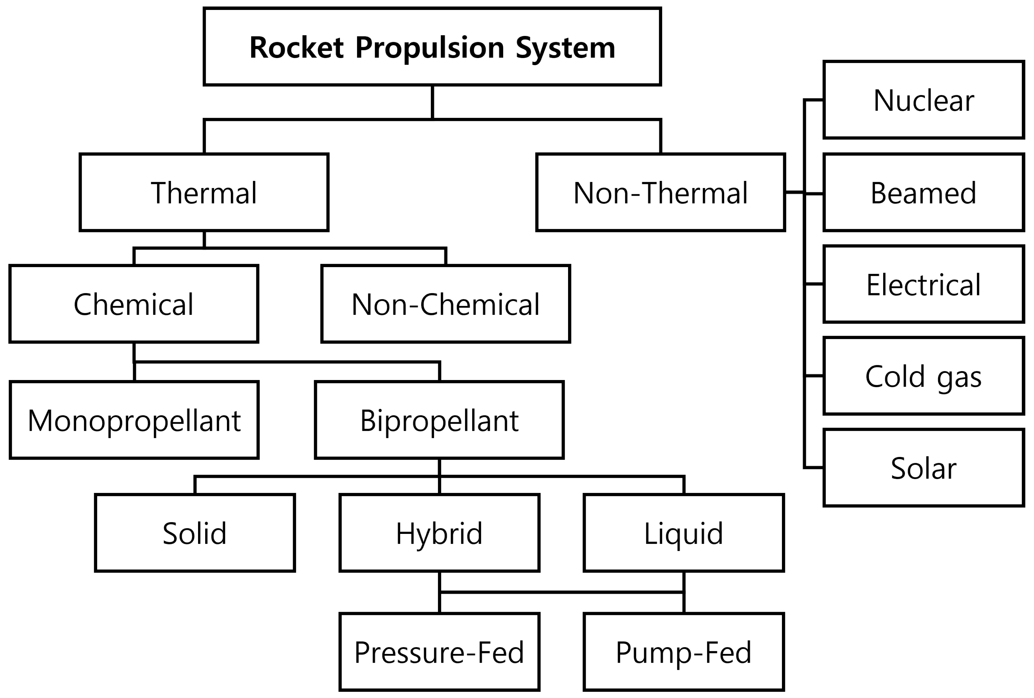
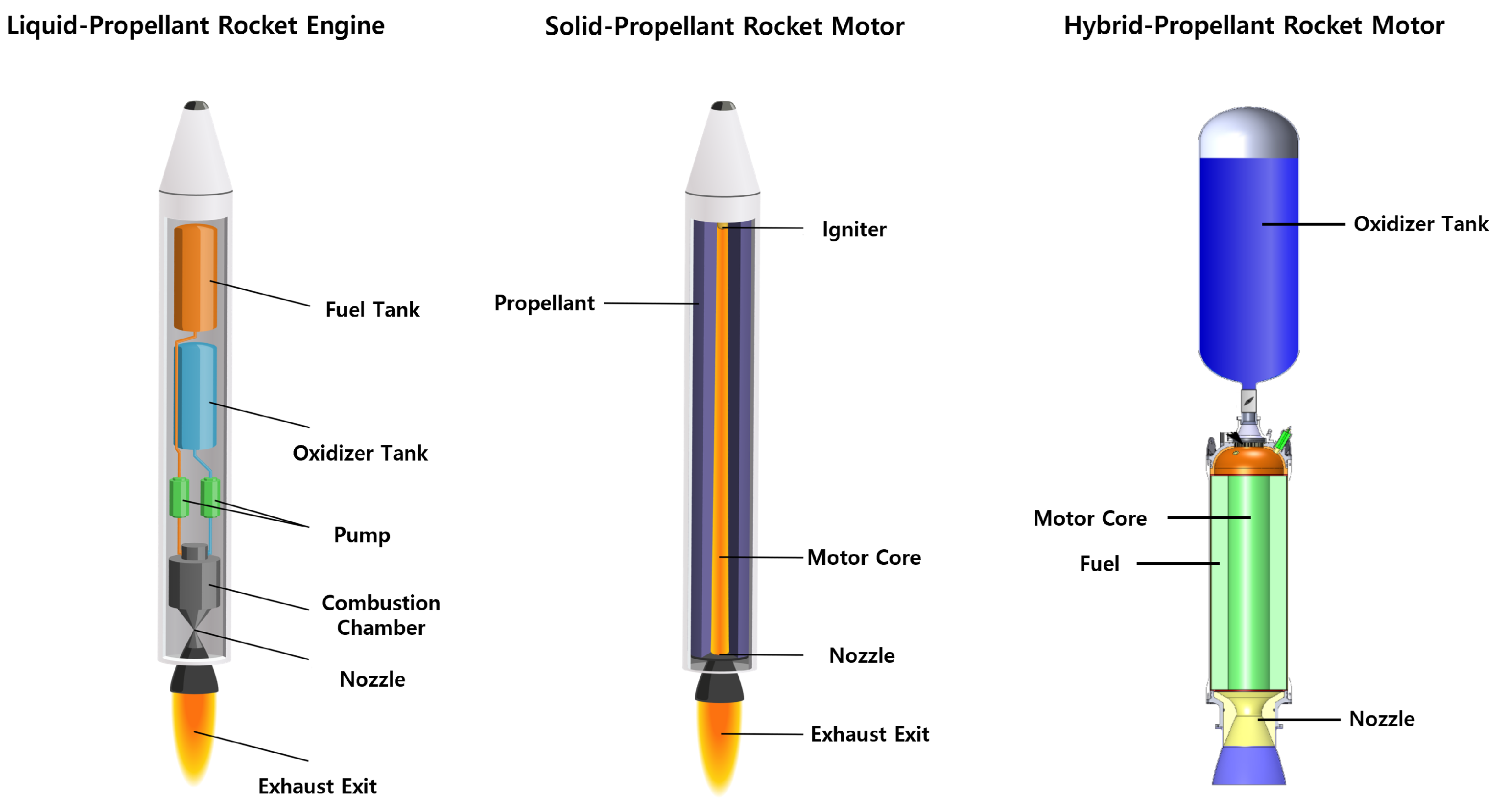
2. Overview of Chemical Propulsion Systems
3. Simulation Modeling Trend of Chemical Propulsion Systems
3.1. Literature Review
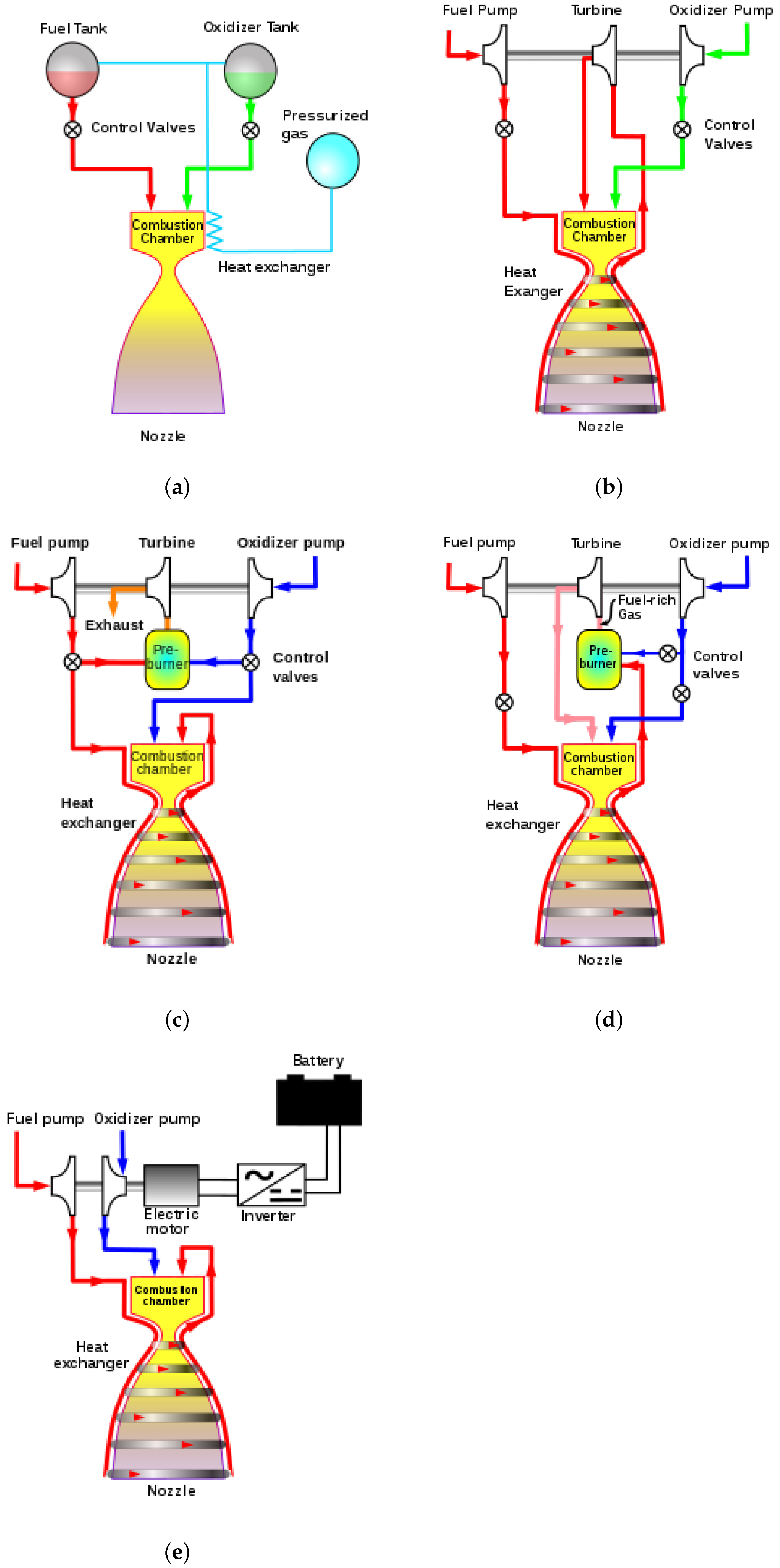
3.1.1. Liquid-Propellant Rocket Engines
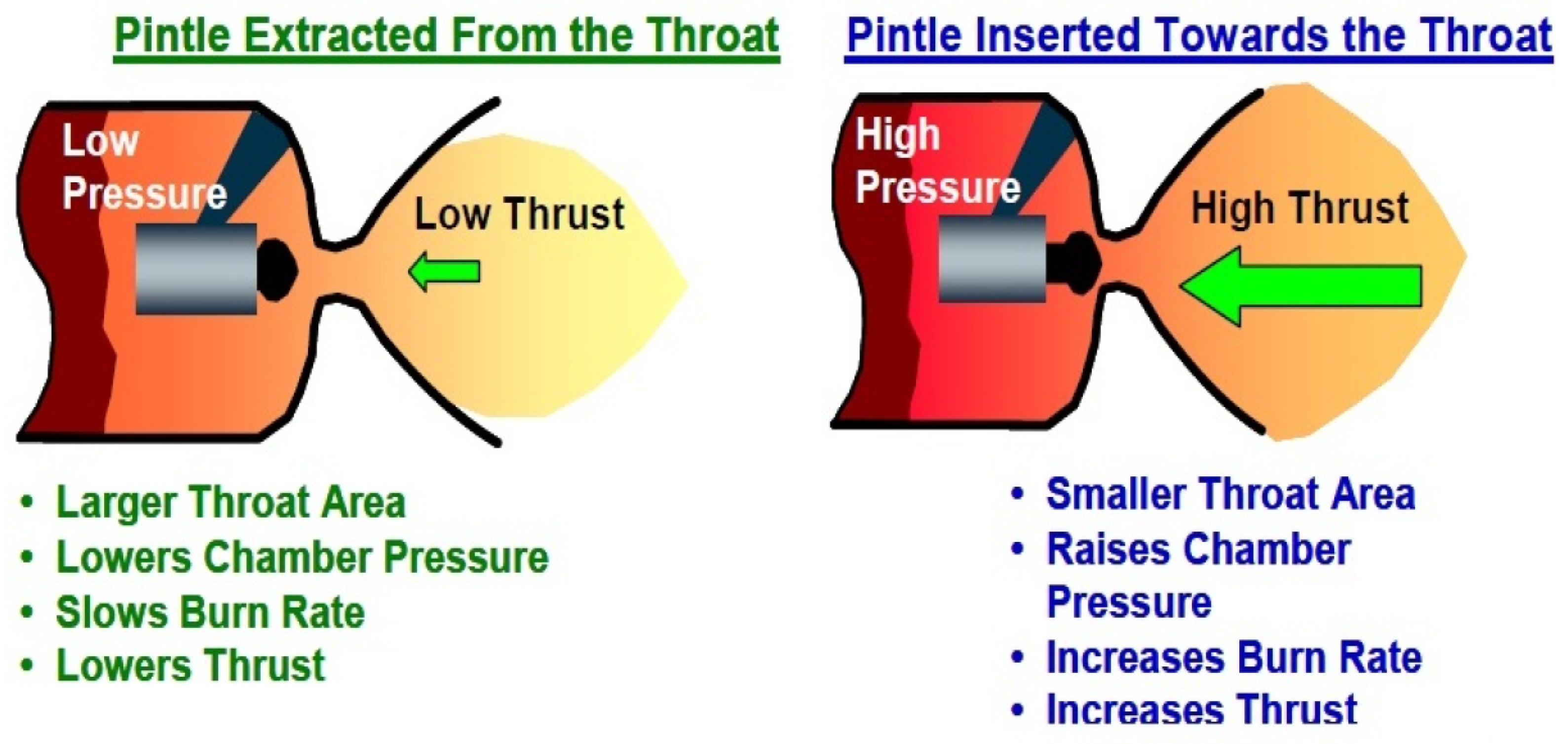
3.1.2. Solid-Propellant Rocket Motor
3.1.3. Hybrid-Propellant Rocket Motor
3.1.4. State of a Chemical Propulsion System
3.2. Analysis of the Trend
3.2.1. Perspective of the Modeling Approach
- Nonlinear modeling: In general, nonlinear modeling of CPS models has been used for simulation and analysis. The physics of propulsion system components are generally described using thermo-fluid-dynamic and mechanical conservation equations. Each component is usually not developed to its full complexity since the most accurate model is not the target. The main input data to the model are propellant tank outlet pressure and temperature, geometric and thermal properties, and valve settings. CPS parameters are initially set using design points determined in preliminary design and critical design. After that, they are upgraded and tuned through estimation through generalized residual sum of squares using data obtained from actual tests.
- Linearized modeling: Linearized modeling is the most common modeling by linearizing a nonlinear thermodynamic model (mostly for design control). The approach is linearized around the design points or previously computed equilibrium points. Generally, after each component of a CPS is linearized based on the equilibrium points, all linearized models are combined. However, sometimes parts of all components, which are nonlinear equations that are hard to describe due to complexity or data lack problems, are linearized and combined with other nonlinear forms to make them simple.
- Linear identification: Some researchers have determined a mathematical model using the data obtained from system-level simulations or actual tests rather than developing a model based on thermodynamic equations. The approach mainly considers each valve opening angle as an input and pressure, temperature, and turbopump speed as outputs. The approach requires preliminary information about the nonlinearity and bandwidth of the system. The responses point to valve nonlinearity, which can be isolated and removed to identify the main system. Through this work, the equations by linear identification have the transfer-function structure between the jth input and the ith output as:where , , and are the standard state-space matrices and s is the Laplace variable. To determine the transfer function coefficients, mostly the recursive maximum likelihood method (RML) or least-square method (LS) are used by subtracting the nominal values from the perturbed data after defining the order of the model.
- Nonlinear identification: There are several nonlinear identification approaches, including the Volterra series model, block-structured model, neural network model, NARMAX model, and state-space model [125]. However, in the five models, mostly a CPS is modeled using an artificial neural network (ANN) approach, which is adequate for real-time monitoring, diagnosis, and control. Using the ANN approach to represent a CPS requires training with a database from actual tests to provide the correct output determined by the user.

| Modeling Approach | Types | Refs. (Selected) |
|---|---|---|
| Nonlinear modeling | LPRE | [16,34,39,40,53,57,60,61,67] |
| SPRM | [77,78,79,84,87] | |
| HPRM | [96,98,99,100] | |
| Linearized modeling | LPRE | [55,126,127] |
| SPRM | [128] | |
| HPRM | [97,129,130] | |
| Linear identification | LPRE | [131,132,133] |
| SPRM | [134] | |
| HPRM | [105,111] | |
| Neural network approach | LPRE | [135,136] |
| SPRM | [137,138] | |
| HPRM | [139,140] |
3.2.2. Perspective of Pipe Modeling Method
| Method | Refs. (Selected) |
|---|---|
| Lumped model method | [34,40,60,67] |
| Method of characteristics | [37,141] |
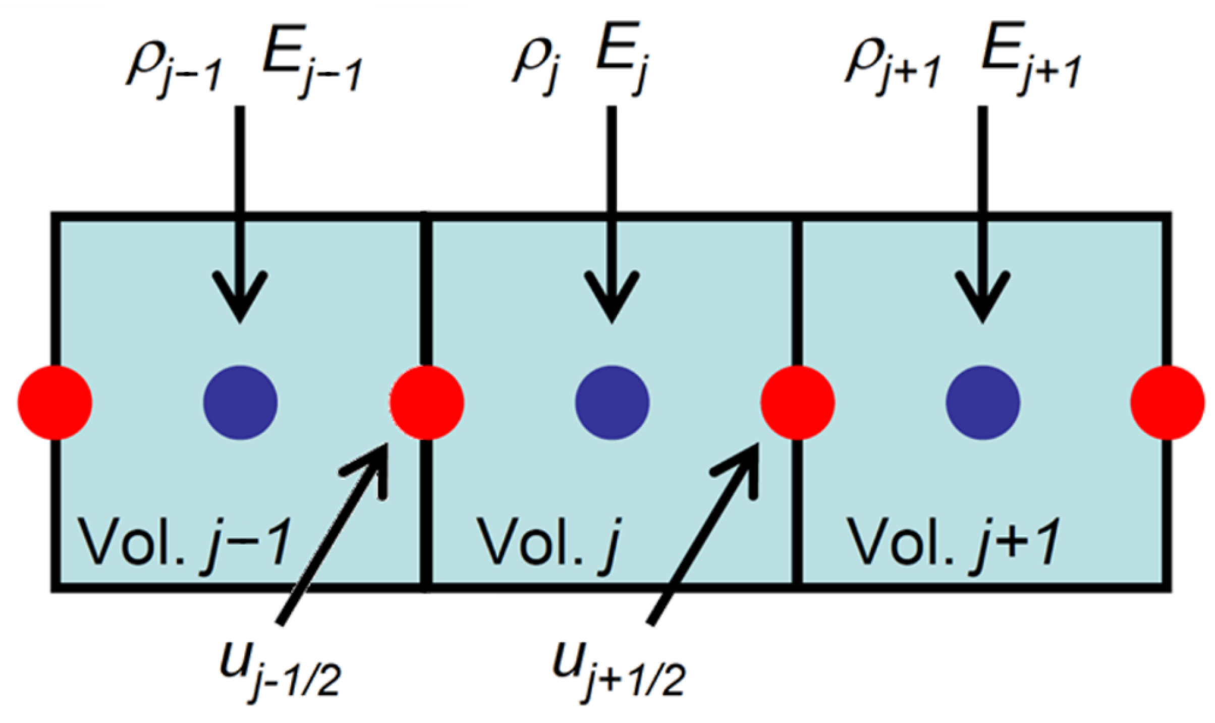
| Volume-junction method (Lumped parameter method) | [29,39,47,142] |
3.2.3. Others
| Country | Institute | Simulation Toolbox | Refs. (Selected) |
|---|---|---|---|
| U.S. | NASA | ROCETS | [28] |
| Europe | ESA | EcosimPro + ESPSS | [31,32] |
| China | NUDT | LRETMMSS | [47] |
| China | HUST | Self-developed Toolbox (Modelica) | [48] |
| China | BUAA | Self-developed Toolbox (MATLAB) | [52] |
| Iran | KNTU | Self-developed Toolbox (MATLAB) | [52] |
| Korea | KAU | Self-developed Toolbox (MATLAB) | [61,62] |
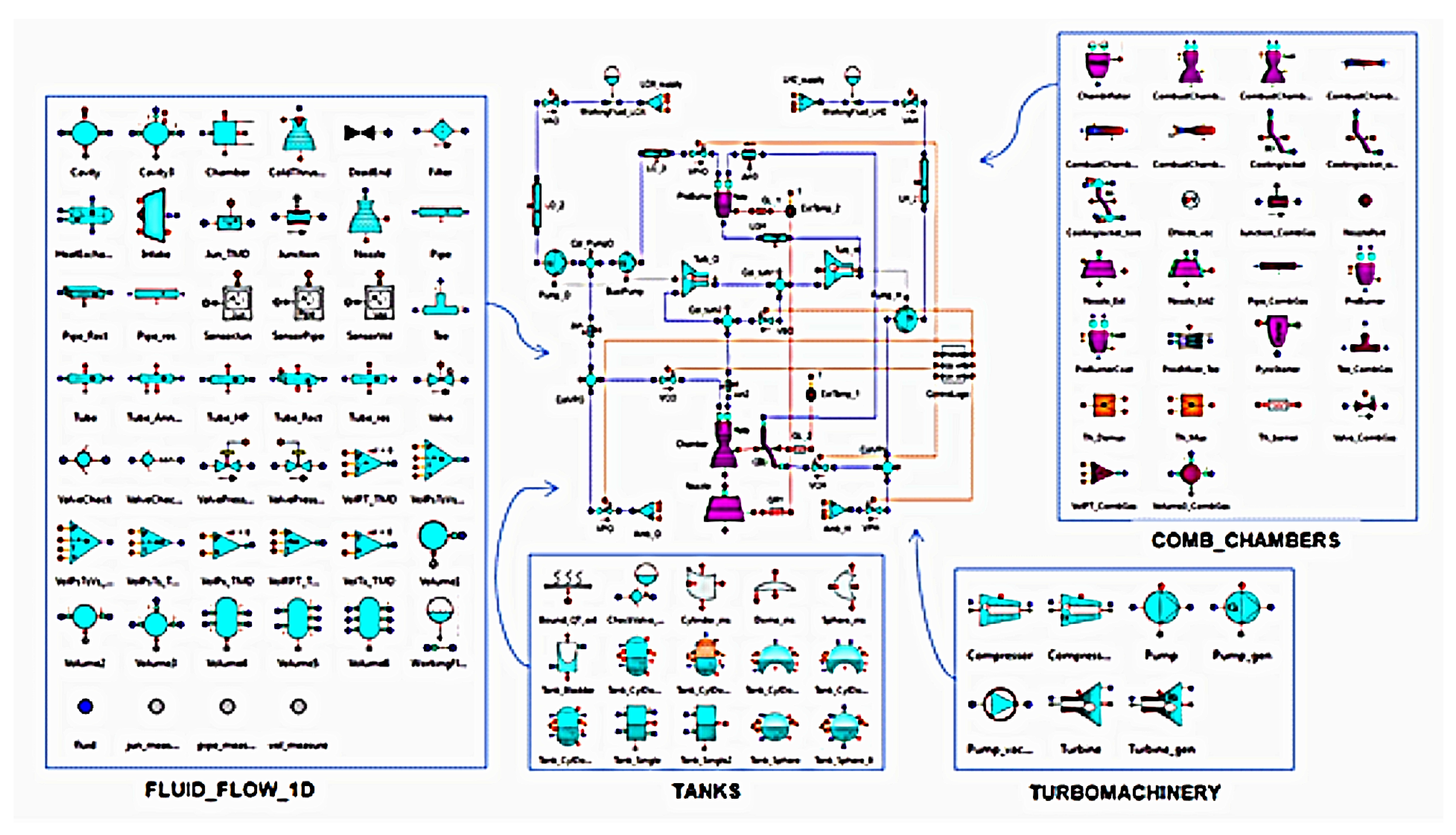
| Main Category | Subcategory | Subsubcategory |
|---|---|---|
| Fluid Properties | - | Ideal gas, Simplified liquids, Real fluids |
| Fluid Flow 1D | AbstracJunction | Jun_TMD, DeadEnd, Filter |
| Time dependent Boundaries | VolPT_TMD, VolPx_TMD, VolTx_TMD | |
| Cavities | Chamber, Volume1, Volume2, Volume5 | |
| AbstacJunctionLoss | Juntion, ValveCheck, Valve, ValvePressRegDown, VallvePressRegUp, ValveCheck_Dynamic, VolPsTsVs_TMD | |
| Sensor | SensorJun, SensorPipe, SensorVol | |
| Channel | Pipe, Tube, Pipe_res, Pipe_Rect, Tube_Rect | |
| Etc. | WorkingFluid, VTee, WorkingFluuid, HeatExchanger, Nozzle, ColdThruster | |
| Tanks | Propellent Tank | Tank_single, Tank_Sphere, Cylinder_ins, Sphere_ins, Tank_CylDomes, Dome_ins, Tank_Bladder, Tank_CylDomesSph |
| Combustion Chambers | Combustor | ABS-Combustor_eq, ABS−Combustor_rate |
| Preburner | PreBurnerCoat_eq, PreBurner_eq, PreBurner_rate, reBurnerCoat_rate | |
| Nozzle | Nozzle, Nozzle_Ex, Nozzle_Ex2 | |
| CobustChamber_Nozzle | CombustChamberNozzle_eq, CombustChambbeerNozzleCoat_eq, CombustChamberNozzle_rate, CombustChambberNozzleCoat_rate | |
| Cooling Jacket | CoolingJacket, CoolingJacket_simple, CoolingJacket_tore | |
| Injector | - | |
| Turbo Machinery | Compressor | Compressor, Compressor_gen |
| Pump | Pump, Pump_gen, Pump_vaccum | |
| Turbine | Turbine, Turbine_gen |

4. Fundamental Mathematical Modeling Approach
4.1. Governing Equations
4.1.1. Rotational Dynamics
4.1.2. Mass Flow Rate
4.1.3. Pressure Dynamics
4.1.4. Density Equation
4.1.5. Energy Balance in Heat Exchangers
4.1.6. Heat Transfer Equations
4.1.7. Time Delay Equation
4.2. Algebraic Equations
4.2.1. The Combustion Gas Mass Flow Rate
4.2.2. Injector Pressure Decremental Equation
4.2.3. The Power or Torque of the Pump
4.2.4. The Power or Torque of the Turbine and Motor
4.3. Characteristics Equations
4.3.1. Pump Pressure Incremental Equation
4.3.2. Propellant State Equation
4.4. Mathematical Modeling of Chemical Propulsion Systems
5. Conclusions
Author Contributions
Funding
Data Availability Statement
Conflicts of Interest
Abbreviations
| A | Cross-area of pipe |
| Burning surface area of solid propellant | |
| Nozzle throat area | |
| , , | Coefficients of pump |
| Discharge coefficient | |
| Torque coefficient of motor | |
| D | Diameter of pipe |
| Moment of inertia of pump rotor | |
| K | Resistance coefficient of pipe |
| Injector resistance coefficient | |
| Resistance coefficient | |
| Coefficient of state change | |
| L | Length of pipe |
| Oxidizer to fuel mixture ratio | |
| P | Pressure |
| Combustion chamber pressure | |
| Inlet pressure | |
| Outlet pressure | |
| Turbine outlet pressure | |
| Turbine inlet pressure | |
| Injector pressure decrement | |
| Pump pressure increment | |
| Q | Flow rate |
| Heat flow rate between the walls and the coolant fluid | |
| Heat flow rate between the hot fluid and the wall | |
| R | Gas constant |
| Gas constant of combustion gas | |
| T | Temperature |
| Temperature of combustion gas | |
| Hot wall temperature | |
| V | Volume |
| Volume of combustion chamber | |
| Power of pump | |
| Power of turbine | |
| Pipe volume ratio of total and filled | |
| a | Speed of sound |
| Empirical constant | |
| Acceleration of vehicle | |
| Specific heat of the wall material | |
| f | Friction factor of pipeline |
| h | Enthalpy of fluid |
| Current of motor | |
| Heat specific ratio of combustion gas | |
| m | Mass of the wall |
| Mass flow rate in pipe | |
| Combustion gas mass flow rate | |
| Injector mass flow rate | |
| Inlet mass flow rate | |
| Outlet mass flow rate | |
| Mass flow rate in pump | |
| Mass flow rate in turbine | |
| n | Burning rate exponent |
| Burning rate | |
| Ignition time | |
| u | Internal energy of fluid |
| Amount of the time delay | |
| Pump efficiency | |
| Turbine efficiency | |
| Fluid compressibility | |
| Density of fluid | |
| Torque produced by turbine or motor | |
| Torque of motor | |
| Torque absorbed by pump | |
| Torque of pump | |
| Torque of turbine | |
| Angular velocity of pump |
References
- Muelhaupt, T.J.; Sorge, M.E.; Morin, J.; Wilson, R.S. Space traffic management in the new space era. J. Space Saf. Eng. 2019, 6, 80–87. [Google Scholar] [CrossRef]
- Kuntanapreeda, S.; Hess, D. Opening access to space by maximizing utilization of 3D printing in launch vehicle design and production. Appl. Sci. Eng. Prog. 2021, 14, 143–145. [Google Scholar] [CrossRef]
- Wekerle, T.; Pessoa, J.B.; Costa, L.E.V.L.d.; Trabasso, L.G. Status and trends of smallsats and their launch vehicles—An up-to-date review. J. Aerosp. Technol. Manag. 2017, 9, 269–286. [Google Scholar] [CrossRef]
- Jones, H. The recent large reduction in space launch cost. In Proceedings of the 48th International Conference on Environmental Systems, Albuquerque, NM, USA, 8–12 July 2018. [Google Scholar]
- Kim, C.T.; Yang, I.; Lee, K.; Lee, Y. Technology Development Prospects and Direction of Reusable Launch Vehicles and Future Propulsion Systems. J. Korean Soc. Aeronaut. Space Sci. 2016, 44, 686–694. [Google Scholar]
- Choo, K.; Mun, H.; Nam, S.; Cha, J.; Ko, S. A survey on recovery technology for reusable space launch vehicle. J. Korean Soc. Propuls. Eng. 2018, 22, 138–151. [Google Scholar] [CrossRef]
- Kim, C.; Lim, B.; Lee, K.; Park, J. A Study on Fuel Selection for Next-Generation Launch Vehicles. J. Korean Soc. Propuls. Eng. 2021, 25, 62–80. [Google Scholar] [CrossRef]
- Bae, J.; Koo, J.; Yoon, Y. Development trend of low cost space launch vehicle and consideration of next generation fuel. J. Korean Soc. Aeronaut. Space Sci. 2017, 45, 855–862. [Google Scholar] [CrossRef]
- Schmierer, C.; Kobald, M.; Tomilin, K.; Fischer, U.; Schlechtriem, S. Low cost small-satellite access to space using hybrid rocket propulsion. Acta Astronaut. 2019, 159, 578–583. [Google Scholar] [CrossRef]
- Yu, B.; Kwak, H.D.; Kim, H.J. Effects of the O/F Ratio on the Performance of a Low Thrust LO X/Methane Rocket Engine with an ElecPump-fed Cycle. Int. J. Aeronaut. Space Sci. 2020, 21, 1037–1046. [Google Scholar] [CrossRef]
- Kawatsu, K.; Tsutsumi, S.; Hirabayashi, M.; Sato, D. Model-based fault diagnostics in an electromechanical actuator of reusable liquid rocket engine. In Proceedings of the AIAA Scitech 2020 Forum, Orlando, FL, USA, 6–10 January 2020; p. 1624. [Google Scholar]
- Satoh, D.; Tsutsumi, S.; Hirabayashi, M.; Kawatsu, K.; Kimura, T. Estimating model parameters of liquid rocket engine simulator using data assimilation. Acta Astronaut. 2020, 177, 373–385. [Google Scholar] [CrossRef]
- Cha, J.; Ha, C.; Ko, S. A survey on health monitoring and management technology for liquid rocket engines. J. Korean Soc. Propuls. Eng. 2014, 18, 50–58. [Google Scholar] [CrossRef]
- Cha, J.; Ha, C.; Koo, J.; Ko, S. Dynamic simulation and analysis of the space shuttle main engine with artificially injected faults. Int. J. Aeronaut. Space Sci. 2016, 17, 535–550. [Google Scholar] [CrossRef]
- Lee, K.; Cha, J.; Ko, S. A Survey on Fault Detection and Diagnosis Method for Open-Cycle Liquid Rocket Engines through China R&D Case. J. Aerosp. Syst. Eng. 2017, 11, 22–30. [Google Scholar]
- Cha, J. Transient State Modeling, Simulation, and Fault Detection/Diagnosis of an open-cycle Liquid Rocket Engine. Ph.D. Thesis, Department of Aerospace and Mechanical Engineering, Republic of Korea Aerospace University, Goyang, Republic of Korea, 2019. [Google Scholar]
- Lee, J.; Cha, S.W.; Ha, D.; Kee, W.; Lee, J.; Huh, H.; Roh, T.S.; Lee, H.J. Research trend analysis on modeling and simulation of liquid propellant supply system. J. Korean Soc. Propuls. Eng. 2019, 23, 39–50. [Google Scholar] [CrossRef]
- Wang, T.; Ding, L.; Yu, H. Research and development of fault diagnosis methods for liquid rocket engines. Aerospace 2022, 9, 481. [Google Scholar] [CrossRef]
- Sutton, G.P.; Biblarz, O. Rocket Propulsion Elements; John Wiley & Sons: Hoboken, NJ, USA, 2016. [Google Scholar]
- Humble, R.W.; Gary, H.N.; Larson, W.J. Space Propulsion Analysis and Design; McGraw-Hill Companies: New York, NY, USA, 1995. [Google Scholar]
- Taylor, T.S. Introduction to Rocket Science and Engineering; CRC Press: Boca Raton, FL, USA, 2017. [Google Scholar]
- El-Sayed, A.F. Fundamentals of Aircraft and Rocket Propulsion; Springer: Berlin/Heidelberg, Germany, 2016. [Google Scholar]
- Huzel, D.K. Modern Engineering for Design of Liquid-Propellant Rocket Engines; AIAA: Reston, VA, USA, 1992; Volume 147. [Google Scholar]
- Davenas, A. Solid Rocket Propulsion Technology; Pergamon Press: Oxford, UK, 2012. [Google Scholar]
- Kuo, K.K.; Chiaverini, M.J. Fundamentals of Hybrid Rocket Combustion and Propulsion; American Institute of Aeronautics and Astronautics: Reston, VA, USA, 2007. [Google Scholar]
- Kalnin, V.; Sherstiannikov, V. Hydrodynamic modelling of the starting process in liquid-propellant engines. Acta Astronaut. 1981, 8, 231–242. [Google Scholar] [CrossRef]
- Harland, D.M.; Lorenz, R. Space Systems Failures: Disasters and Rescues of Satellites, Rocket and Space Probes; Springer Science & Business Media: Berlin/Heidelberg, Germany, 2007. [Google Scholar]
- Mason, J.; Southwick, R. Large Liquid Rocket Engine Transient Performance Simulation System; Technical Report; The National Aeronautics and Space Administration: Huntsville, AL, USA, 1991.
- Yamanishi, N.; Kimura, T.; Takahashi, M.; Okita, K.; Atsumi, M.; Negishi, H. Transient analysis of the LE-7A rocket engine using the rocket engine dynamic simulator (REDS). In Proceedings of the 40th AIAA/ASME/SAE/ASEE Joint Propulsion Conference and Exhibit, Fort Lauderdale, FL, USA, 11–14 July 2004; p. 3850. [Google Scholar]
- Francesco, D.M. Modelling and Simulation of Liquid Rocket Engine Ignition Transients. Ph.D. Thesis, Department of Aeronautics and Space Engineering, Sapienza University of Rome, Roma, Italy, 2011. [Google Scholar]
- Moral, J.; Pérez Vara, R.; Steelant, J.; De Rosa, M. ESPSS Simulation Platform. In Proceedings of the Space Propulsion 2010, San Sebastian, Spain, 3–6 May 2010. [Google Scholar]
- Moral, J.; Rodríguez, F.; Vilá, J.; Di Matteo, F.; Steelant, J. 1-D Simulation of Solid and Hybrid Combustors with EcosimPro/ESPSS. In Proceedings of the Space Propulsion 2014, Cologne, Germany, 19–22 May 2014; pp. 19–22. [Google Scholar]
- Unit, H.S.A.; Unit, S.D. Engine Balance and Dynamics Model; Technical Report; Report Number RL00001; Rockwell International Corporation, Rocket Dyne Division: Oshkosh, WI, USA, 1992. [Google Scholar]
- Lozano-Tovar, P.C. Dynamic Models for Liquid Rocket Engines with Health Monitoring Application. Master’s Thesis, Department of Aeronautics and Astronautics, Massachusetts Institute of Technology, Cambridge, MA, USA, 1998. [Google Scholar]
- Ho, N.T. Failure Detection and Isolation for the Space Shuttle Main Engine. Master’s Thesis, Department of Mechanical Engineering, Massachusetts Institute of Technology, Cambridge, MA, USA, 1998. [Google Scholar]
- Ho, N.; Lozano, P.; Martinez-Sanchez, M.; Mangoubi, R.; Ho, N.; Lozano, P.; Martinez-Sanchez, M.; Mangoubi, R. Failure detection and isolation for the Space Shuttle Main Engine. In Proceedings of the 33rd Joint Propulsion Conference and Exhibit, Seattle, WA, USA, 6–9 July 1997; p. 2821. [Google Scholar]
- Ruth, E.; Ahn, H.; Baker, R.; Brosmer, M. Advanced liquid rocket engine transient model. In Proceedings of the 26th Joint Propulsion Conference, Orlando, FL, USA, 16–18 July 1990; p. 2299. [Google Scholar]
- Manfletti, C. Start-Up Transient Simulation of a Pressure Fed LOx/LH2 Upper Stage Engine Using the Lumped Parameter-based MOLIERE Code. In Proceedings of the 46th Joint Propulsion Conference & Exhibit, Nashville, TN, USA, 25–28 July 2010. [Google Scholar]
- Manfletti, C. Transient Behaviour Modeling of Liquid Rocket Engine Components. Ph.D. Thesis, Aerospace, Aeronautical and Astronautical/Space Engineering, RWTH Aachen University, Aachen, German, 2010. [Google Scholar]
- Pérez-Roca, S.; Marzat, J.; Piet-Lahanier, H.; Langlois, N.; Galeotta, M.; Farago, F.; Le Gonidec, S. Model-based robust transient control of reusable liquid-propellant rocket engines. IEEE Trans. Aerosp. Electron. Syst. 2020, 57, 129–144. [Google Scholar] [CrossRef]
- Pérez-Roca, S. Model-based Robust Transient Control of Reusable Liquid-Propellant Rocket Engines Transient Behaviour Modeling of Liquid Rocket Engine Components. Ph.D. Thesis, University of Paris-Saclay, Paris, France, 2020. [Google Scholar]
- Lebedinsky, E.; Mosolov, S.; Kalmykov, G.; Zenin, E.; Tararyshkin, V.; Fedotchev, V. Computer Models of Liquid-Propellant Rocket Engines; Mashinostroenie: Moscow, Russia, 2009. [Google Scholar]
- Belyaev, E.; Chvanov, V.; Chervakov, V. Mathematical Modeling Workflow Liquid Rocket Engines; Moscow Aviation Institution: Moscow, Russia, 1999. [Google Scholar]
- Wu, J.; Zhang, Y.; Chen, Q. Transient performance simulation of a large liquid rocket engine under fault conditions. J. Aerosp. Power China 1994, 9, 361–365. [Google Scholar]
- Wu, J.; Zhang, Y.; Chen, Q. Steady fault simulation and analysis of liquid rocket engine. J. Propuls. Technol. China 1994, 15, 6–13. [Google Scholar]
- Zhang, Y.; Wu, J.; Huang, M.; Zhu, H.; Chen, Q. Liquid-propellant rocket engine health-monitoring techniques. J. Propuls. Power 1998, 14, 657–663. [Google Scholar] [CrossRef]
- Liu, K.; Zhang, Y. A study on versatile simulation of liquid propellant rocket engine systems transients. In Proceedings of the 36th AIAA/ASME/SAE/ASEE Joint Propulsion Conference and Exhibit, Huntsville, AL, USA, 17–19 July 2000; p. 3771. [Google Scholar]
- Wei, L.; Liping, C.; Gang, X.; Ji, D.; Haiming, Z.; Hao, Y. Modeling and simulation of liquid propellant rocket engine transient performance using modelica. In Proceedings of the 11th International Modelica Conference, Versailles, France, 21–23 September 2015; pp. 485–490. [Google Scholar]
- Zheng, Y.; Tong, X.; Cai, G.; Chen, J. Simulation and optimization of liquid propellants rocket engine for system design. J. Beijing Univ. Aeronaut. Astronaut. 2006, 32, 40–45. [Google Scholar]
- Zhu, S. H2/O2 Rocket Engine and Cryogenic Technique; National Defense Industry Press: Beijing, China, 1995; pp. 15–17. [Google Scholar]
- Cai, G.; Fang, J.; Zheng, Y.; Tong, X.; Chen, J.; Wang, J. Optimization of system parameters for liquid rocket engines with gas-generator cycles. J. Propuls. Power 2010, 26, 113–119. [Google Scholar] [CrossRef]
- Naderi, M.; Liang, G.; Karimi, H. Modular simulation software development for liquid propellant rocket engines based on MATLAB Simulink. In Proceedings of the MATEC Web of Conferences. EDP Sciences, Beijing, China, 12–14 May 2017; Volume 114, p. 02010. [Google Scholar]
- Naderi, M.; Liang, G. Static performance modeling and simulation of the staged combustion cycle LPREs. Aerosp. Sci. Technol. 2019, 86, 30–46. [Google Scholar] [CrossRef]
- Mota, F.A.d.S.; Hinckel, J.N.; Rocco, E.M.; Schlingloff, H. Modeling and analysis of a LOX/Ethanol liquid rocket engine. J. Aerosp. Technol. Manag. 2018, 10, e3018. [Google Scholar] [CrossRef]
- Park, S.Y.; Cho, W.K.; Seol, W.S. A Mathematical Model of Liquid Rocket Engine Using Simulink. Aerosp. Eng. Technol. 2009, 8, 82–97. [Google Scholar]
- Jung, T. Development and evaluation of startup simulation code for an open cycle liquid rocket engine. J. Korean Soc. Propuls. Eng. 2019, 23, 67–74. [Google Scholar] [CrossRef]
- Jung, T. Transient Mathematical Modeling and Simulation for an Open Cycle Liquid Rocket Engine. In Proceedings of the Asia-Pacific International Symposium on Aerospace Technology, Jeju, Republic of Korea, 15–17 November 2021; pp. 1343–1360. [Google Scholar]
- Yeon, K.B.; Insang, M. Study on Energy Balance at the Operating Points of Staged Combustion Cycle LRE. Int. J. Aeronaut. Space Sci. 2023, 1–9. [Google Scholar] [CrossRef]
- Ha, C.; O, S.; Cha, J.; Ko, S. Basic modeling and analysis for the operation of Space Shuttle Main Engine. In Proceedings of the Korean Society for Aeronautical and Space Sciences Fall Conference, Jeju, Republic of Korea, 19–21 November 2014; pp. 1573–1576. [Google Scholar]
- Lee, K.; Cha, J.; Ko, S.; Park, S.Y.; Jung, E. Mathematical modeling and simulation for steady state of a 75-ton liquid propellant rocket engine. J. Aerosp. Syst. Eng. 2017, 11, 6–12. [Google Scholar]
- Cho, W.; Cha, J.; Ko, S.; Park, S.Y.; Jung, E. Development of MATLAB/Simulink Modular Simulation Environment for Open-cycle Liquid Propellant Rocket Engines. In Proceedings of the Korean Society for Aeronautical and Space Sciences Fall Conference, Jeju, Republic of Korea, 28 November–1 December 2018. [Google Scholar]
- Cho, W.; Cha, J.; Ko, S. Development of MATLAB/Simulink Modular Simulation Toolbox for Space Shuttle Main Engine. J. Korean Soc. Propuls. Eng. 2019, 23, 50–60. [Google Scholar] [CrossRef]
- Lee, S.; Jo, S.; Kim, H.; Kim, S.; Yi, S. A Numerical Study on the Simulation of Power-pack Start-up of a Staged Combustion Cycle Engine. J. Korean Soc. Propuls. Eng. 2019, 23, 58–66. [Google Scholar] [CrossRef]
- Yu, S.; Jo, S.; Kim, H.; Kim, S.L. A 1-D Start-up Analysis for Liquid Rocket Engine Powerpacks. J. Korean Soc. Combust. 2019, 24, 39–45. [Google Scholar] [CrossRef]
- Rachov, P.P.; Tacca, H.; Lentini, D. Electric feed systems for liquid-propellant rockets. J. Propuls. Power 2013, 29, 1171–1180. [Google Scholar] [CrossRef]
- Lee, J.; Roh, T.S.; Huh, H.; Lee, H.J. Performance analysis and mass estimation of a small-sized liquid rocket engine with electric-pump cycle. Int. J. Aeronaut. Space Sci. 2021, 22, 94–107. [Google Scholar] [CrossRef]
- Lee, J. Development of MS Program for Propellant Supply System of a Small-sized LRE with Electric-pump Cycle. Master’s Thesis, Department of Aerospace Engineering, Inha University, Incheon, Republic of Korea, 2021. [Google Scholar]
- Ramesh, D.; Aminpoor, M. Nonlinear, dynamic simulation of an open cycle liquid rocket engine. In Proceedings of the 43rd AIAA/ASME/SAE/ASEE Joint Propulsion Conference & Exhibit, Cincinnati, OH, USA, 8–11 July 2007; p. 5507. [Google Scholar]
- Shafiey Dehaj, M.; Ebrahimi, R.; Karimi, H. Mathematical modeling and analysis of cutoff impulse in a liquid-propellant rocket engine. Proc. Inst. Mech. Eng. Part G J. Aerosp. Eng. 2015, 229, 2358–2374. [Google Scholar] [CrossRef]
- Mahjub, A.; Mazlan, N.M.; Abdullah, M.; Azam, Q. Design optimization of solid rocket propulsion: A survey of recent advancements. J. Spacecr. Rocket. 2020, 57, 3–11. [Google Scholar] [CrossRef]
- McDonald, A. Solid rockets-An affordable solution to future space propulsion needs. In Proceedings of the 20th Joint Propulsion Conference, Cincinnati, OH, USA, 11–13 June 1984; p. 1188. [Google Scholar]
- Kim, Y.S.; Cha, J.H.; Ko, S.H.; Kim, D.S. Control of pressure and thrust for a variable thrust solid propulsion system using linearization. J. Korean Soc. Propuls. Eng. 2011, 15, 18–25. [Google Scholar]
- Caubet, P.; Berdoyes, M. Innovative ArianeGroup Controllable Solid Propulsion Technologies. In Proceedings of the AIAA Propulsion and Energy 2019 Forum, Indianapolis, IN, USA, 19–22 August 2019; p. 3878. [Google Scholar]
- Lombardo, G. Controllable Solid Propellant Rocket Motor Stability: Deep and Rapid Variable Thrust Operations. In Proceedings of the 44th AIAA/ASME/SAE/ASEE Joint Propulsion Conference & Exhibit, Hartford, CT, USA, 21–23 July 2008; p. 4608. [Google Scholar]
- Park, I.S.; Lee, J.Y.; Choi, H.J.; Kim, J.H.; Yoon, H.G.; Lim, J.S. Pressure Control Law of Gas Generator Considering Combustion Volume Change. J. Korean Soc. Propuls. Eng. 2012, 16, 34–40. [Google Scholar]
- Ki, T.; Ha, D.; Jin, J.; Lee, H.; Yoon, H. Analysis of Unsteady Combustion Performance in Solid Rocket Motor with Pintle. J. Korean Soc. Propuls. Eng. 2015, 19, 68–75. [Google Scholar] [CrossRef]
- Hong, S. Gain Scheduling Controller Design and Performance Evaluation for Thrust Control of Variable Thrust Solid Rocket Motor. J. Korean Soc. Propuls. Eng. 2016, 20, 28–36. [Google Scholar] [CrossRef]
- Cha, J.; de Oliveira, É.J. Performance Comparison of Control Strategies for a Variable-Thrust Solid-Propellant Rocket Motor. Aerospace 2022, 9, 325. [Google Scholar] [CrossRef]
- Alan, A.; Yildiz, Y.; Poyraz, U. High-performance adaptive pressure control in the presence of time delays: Pressure control for use in variable-thrust rocket development. IEEE Control Syst. Mag. 2018, 38, 26–52. [Google Scholar] [CrossRef]
- Bergmans, J.L.; Di Salvo, R. Solid rocket motor control: Theoretical motivation and experimental demonstration. In Proceedings of the 39th AIAA/ASME/SAE/ASEE Joint Propulsion Conference & Exhibit, Huntsville, AL, USA, 20–23 July 2003. [Google Scholar]
- Lee, H.S.; Lee, D.Y.; Park, J.S.; Kim, J.K. A Study on Pressure Control for Variable Thrust Solid Propulsion System Using Cold Gas Test Equipment. J. Korean Soc. Aeronaut. Space Sci. 2009, 37, 76–81. [Google Scholar]
- Ko, H.; Lee, J. Cold tests and the dynamic characteristics of the pintle type solid rocket motor. In Proceedings of the 49th AIAA/ASME/SAE/ASEE Joint Propulsion Conference, San Jose, CA, USA, 14–17 July 2013; p. 4079. [Google Scholar]
- Kwon, S.K.; Kim, Y.S.; Ko, S.H.; Suh, S.H. Pressure Control of a Variable Thrust Solid Propulsion System Using On-Off Controllers. In Proceedings of the Korean Society of Propulsion Engineers Conference, Busan, Republic of Korea, 2–24 November 2011; pp. 942–948. [Google Scholar]
- Lee, J. A Study on the Static and Dynamic Characteristics of Pintle-Perturbed Conical Nozzle Flows. Ph.D. Thesis, Department of Mechanical Engineering, Yonsei University Seoul, Seoul, Republic of Korea, 2012. [Google Scholar]
- Napior, J.; Garmy, V. Controllable solid propulsion for launch vehicle and spacecraft application. In Proceedings of the 57th International Astronautical Congress, Valenica, Spain, 2–6 October 2006; p. C4-2. [Google Scholar]
- Lim, Y.; Lee, W.; Bang, H.; Lee, H. Thrust distribution for attitude control in a variable thrust propulsion system with four ACS nozzles. Adv. Space Res. 2017, 59, 1848–1860. [Google Scholar] [CrossRef]
- Lee, H.; Bang, H. Efficient Thrust Management Algorithm for Variable Thrust Solid Propulsion System with Multi-Nozzles. J. Spacecr. Rocket. 2020, 57, 328–345. [Google Scholar] [CrossRef]
- Ji, M.; Chang, H. Modeling and dynamic characteristics analysis on solid attitude control motor using pintle thrusters. Aerosp. Sci. Technol. 2020, 106, 106130. [Google Scholar]
- Park, I.; Hong, S.; Ki, T.; Park, J. Pressure Guidance and Thrust Allocation Law of Solid DACS. J. Korean Soc. Propuls. Eng. 2015, 19, 9–16. [Google Scholar] [CrossRef]
- Ki, T.; Hong, S.; Park, I.S. Dynamic Modeling and Characteristics Analysis of Solid Rocket Motor with Multi Axis Pintle Nozzles. J. Korean Soc. Propuls. Eng. 2015, 19, 20–28. [Google Scholar] [CrossRef]
- Cha, J. A Study on Thrust Control System Design for Multi-Nozzle Solid Propulsion System. Master’s Thesis, Department of Aerospace and Mechanical Engineering, Korea Aerospace University, Goyang, Republic of Korea, 2014. [Google Scholar]
- Alan, A.; Yildiz, Y.; Poyraz, U. Adaptive pressure control experiment: Controller design and implementation. In Proceedings of the 2017 IEEE Conference on Control Technology and Applications (CCTA), Maui, HI, USA, 27–30 August 2017; pp. 80–85. [Google Scholar]
- Yonggang, G.; Yang, L.; Zexin, C.; Xiaocong, L.; Chunbo, H.; Xiaojing, Y. Influence of lobe geometry on mixing and heat release characteristics of solid fuel rocket scramjet combustor. Acta Astronaut. 2019, 164, 212–229. [Google Scholar] [CrossRef]
- Yang, L.; Yonggang, G.; Lei, S.; Zexin, C.; Xiaojing, Y. Preliminary experimental study on solid rocket fuel gas scramjet. Acta Astronaut. 2018, 153, 146–153. [Google Scholar] [CrossRef]
- Chang, J.; Li, B.; Bao, W.; Niu, W.; Yu, D. Thrust control system design of ducted rockets. Acta Astronaut. 2011, 69, 86–95. [Google Scholar] [CrossRef]
- Rezaei, H.; Soltani, M.R. An analytical and experimental study of a hybrid rocket motor. Proc. Inst. Mech. Eng. Part G J. Aerosp. Eng. 2014, 228, 2475–2486. [Google Scholar] [CrossRef]
- Tahmasebi, E.A.; Karimi M, H. Conceptual design and performance simulation of a space hybrid motor. Aircr. Eng. Aerosp. Technol. Int. J. 2015, 87, 92–99. [Google Scholar] [CrossRef]
- Chelaru, T.V.; Mingireanu, F. Hybrid rocket engine, theoretical model and experiment. Acta Astronaut. 2011, 68, 1891–1902. [Google Scholar] [CrossRef]
- Gieras, M.; Gorgeri, A. Numerical modelling of the hybrid rocket engine performance. Propuls. Power Res. 2021, 10, 15–22. [Google Scholar] [CrossRef]
- Cha, J.; Cho, W.; Lee, D.; Moon, H.; Ko, S. Mathematical modeling and simulation of a HDPE/Gox hybrid rocket motor. In Proceedings of the Korean Society for Aeronautical and Space Sciences Spring Conference, Goseong, Republic of Korea, 8–11 July 2020; pp. 310–311. [Google Scholar]
- Tiensuu, K.; Hagel, E.; Bussmann, A.; Liljekvist, F.; Angeria, B.; Borg, L.; Coppa, E.; Gatti, F.; Williamson, A.; Athauda, D.; et al. RAVEN: A student rocket program at Luleå University of Technology, Sweden. In Proceedings of the 72nd International Astronautical Congress (IAC), Dubai, United Arab Emirates, 25–29 October 2021; International Astronautical Federation (IAF): Paris, France, 2021. [Google Scholar]
- Kulu, E. Small launchers-2021 industry survey and market analysis. In Proceedings of the 72th International Astronautical Congress (IAC), Dubai, United Arab Emirates, 25–29 October 2021; International Astronautical Federation (IAF): Paris, France, 2021. [Google Scholar]
- Genevieve, B.; Brooks, M.; Pitot de la Beaujardiere, J.; Roberts, L. Performance modeling of a paraffin wax/nitrous oxide hybrid rocket motor. In Proceedings of the 49th AIAA Aerospace Sciences Meeting including the New Horizons Forum and Aerospace Exposition, Orlando, FL, USA, 4–7 January 2011; p. 420. [Google Scholar]
- Mungas, G.S.; Das, D.K.; Kulkarni, D. Design, construction and testing of a low-cost hybrid rocket motor. Aircr. Eng. Aerosp. Technol. 2003, 75, 262–271. [Google Scholar] [CrossRef]
- Chae, H.; Chae, D.; Rhee, I.; Lee, C. Simulation of response characteristic of VTVL system with hybrid rocket engine. J. Mech. Sci. Technol. 2020, 34, 5239–5245. [Google Scholar] [CrossRef]
- Bhadran, A.; Manathara, J.G.; Ramakrishna, P. Thrust control of lab-scale hybrid rocket motor with wax-aluminum fuel and air as oxidizer. Aerospace 2022, 9, 474. [Google Scholar] [CrossRef]
- Whitmore, S.A.; Peterson, Z.W.; Eilers, S.D. Closed-loop precision throttling of a hybrid rocket motor. J. Propuls. Power 2014, 30, 325–336. [Google Scholar] [CrossRef]
- Velthuysen, T.J. Closed-Loop Throttle Control of a Hybrid Rocket Motor. Master’s Thesis, Department of Mechanical Engineering, University of KwaZulu-Natal, Durban, South Africa, 2018. [Google Scholar]
- Peterson, Z.; Eilers, S.; Whitmore, S. Closed-loop thrust and pressure profile throttling of a nitrous-oxide HTPB hybrid rocket motor. In Proceedings of the 48th AIAA/ASME/SAE/ASEE Joint Propulsion Conference & Exhibit, Atlanta, GA, USA, 30 July–1 August 2012; p. 4200. [Google Scholar]
- Peterson, Z.W. Closed-Loop Thrust and Pressure Profile Throttling of a Nitrous Oxide/Hydroxyl-Terminated Polybutadiene Hybrid Rocket Motor. Master’s Thesis, Department of Aerospace Engineering, Utah State University, Logan, UT, USA, 2012. [Google Scholar]
- Chae, D.; Chae, H.; Lee, C. Controlling plant dynamics change characteristics in thrust response of hybrid rocket engine. J. Mech. Sci. Technol. 2022, 36, 1537–1545. [Google Scholar] [CrossRef]
- Schmierer, C.; Kobald, M.; Steelant, J.; Schlechtriem, S. Combined Trajectory Simulation and Optimization for Hybrid Rockets using ASTOS and ESPSS. In Proceedings of the 31st International Symposium on Space Technology and Science (ISTS), Matsuyama, Japan, 3–9 June 2017. [Google Scholar]
- Rotondi, M.; Concio, P.; D’Alessandro, S.; Lucas, F.R.; Bianchi, D.; Nasuti, F.; Steelant, J. Development and Validation of Nozzle Erosion Models for Solid and Hybrid Rockets in the Espss Libraries. In Proceedings of the Conference: 8th Space Propulsion, Estoril, Portugal, 9–13 May 2022. [Google Scholar]
- Lin, T.; Baker, D. Analysis and testing of propellant feed system priming process. J. Propuls. Power 1995, 11, 505–512. [Google Scholar] [CrossRef]
- Hardi, J.S.; Oschwald, M.; Webster, S.C.; Gröning, S.; Beinke, S.K.; Armbruster, W.; Blanco, P.N.; Suslov, D.; Knapp, B. High frequency combustion instabilities in liquid propellant rocket engines: Research programme at DLR Lampoldshausen. In Proceedings of the Thermoacoustic Instabilities in Gas Turbines and Rocket Engines: Industry Meets Academia, Munich, Germany, 30 May–2 June 2016; pp. 1–11. [Google Scholar]
- Schmidt, V.; Klimenko, D.; Haidn, O.; Oschwald, M.; Nicole, A.; Ordonneau, G.; Habbibalah, M. Experimental investigation and modelling of the ignition transient of a coaxial H2/O2-injector. In Proceedings of the 5th International Symposium on Liquid Rocket Propulsion, Chattanooga, TN, USA, 27–31 October 2003. [Google Scholar]
- Bradley, M.; Bradley, M. Start with off-nominal propellant inlet pressures. In Proceedings of the 33rd Joint Propulsion Conference and Exhibit, Seattle, WA, USA, 6–9 July 1997; p. 2687. [Google Scholar]
- Nam, C.H.; Park, S.Y. Gas Generator Cycle Liquid Rocket Engine Powerpack Startup Behavior Comparison by Valve Operation Order. In Proceedings of the Korean Society of Propulsion Engineers Fall Conference, Gyeongju, Republic of Korea, 5–6 December 2013; The Korean Society of Propulsion Engineers: Daejeon, Republic of Korea, 2013; pp. 560–566. [Google Scholar]
- Park, S.Y.; Cho, W.K. Dispersion Analysis on the Startup and Shutdown Process of a Liquid Rocket Engine using Monte-Carlo Method. In Proceedings of the Korean Society of Propulsion Engineers Spring Conference, Busan, Republic of Korea, 28–29 May 2015; The Korean Society of Propulsion Engineers: Daejeon, Republic of Korea; pp. 787–791. [Google Scholar]
- Cha, J.; Ko, S.; Park, S.Y.; Jeong, E. Fault detection and diagnosis algorithms for transient state of an open-cycle liquid rocket engine using nonlinear Kalman filter methods. Acta Astronaut. 2019, 163, 147–156. [Google Scholar] [CrossRef]
- Wang, T.S. Transient two-dimensional analysis of side load in liquid rocket engine nozzles. In Proceedings of the 40th AIAA/ASME/SAE/ASEE Joint Propulsion Conference and Exhibit, Fort Lauderdale, FL, USA, 11–14 July 2004; p. 3680. [Google Scholar]
- Wang, T.S. Transient three-dimensional startup side load analysis of a regeneratively cooled nozzle. Shock Waves 2009, 19, 251–264. [Google Scholar] [CrossRef]
- Tomita, T.; Sakamoto, H.; Onodera, T.; Sasaki, M.; Takahashi, M.; Watanabe, Y.; Tamura, H. Experimental Evaluation of Side-load Characteristics on TP, CTP and TO nozzles. In Proceedings of the 40th AIAA/ASME/SAE/ASEE Joint Propulsion Conference and Exhibit, Fort Lauderdale, FL, USA, 11–14 July 2004; p. 3678. [Google Scholar]
- Pérez-Roca, S.; Marzat, J.; Piet-Lahanier, H.; Langlois, N.; Farago, F.; Galeotta, M.; Le Gonidec, S. A survey of automatic control methods for liquid-propellant rocket engines. Prog. Aerosp. Sci. 2019, 107, 63–84. [Google Scholar] [CrossRef]
- Nelles, O. Nonlinear System Identification: From Classical Approaches to Neural Networks, Fuzzy Systems, and Gaussian Processes; Springer Nature: Berlin/Heidelberg, Germany, 2020. [Google Scholar]
- Santana, A., Jr.; Barbosa, F.; Niwa, M.; Goes, L. Modeling and robust analysis of a liquid rocket engine. In Proceedings of the 36th AIAA/ASME/SAE/ASEE Joint Propulsion Conference and Exhibit, Huntsville, AL, USA, 16–19 July 2000; p. 3160. [Google Scholar]
- Santana, A.; Goes, L. Design and Dynamic Characteristics of a Liquid-Propellant Thrust Chamber. In Proceedings of the National Conference on Mechanical Engineering, Calcutta, India, 20–22 January 2000. [Google Scholar]
- Jung, J.H. Modeling, and Classical and Advanced Control of a Solid Rocket Motor Thrust Vector Control System. Master’s Thesis, Department of Electrical Engineering and Computer Science, Massachusetts Institute of Technology, Cambridge, MA, USA, 1993. [Google Scholar]
- Karabeyoglu, M.A.; Altman, D. Dynamic modeling of hybrid rocket combustion. J. Propuls. Power 1999, 15, 562–571. [Google Scholar] [CrossRef]
- Antoniou, A.; Akyuzlu, K. A physics based comprehensive mathematical model to predict motor performance in hybrid rocket propulsion systems. In Proceedings of the 41st AIAA/ASME/SAE/ASEE Joint Propulsion Conference & Exhibit, Tucson, AZ, USA, 10–13 July 2005; p. 3541. [Google Scholar]
- Duyar, A.; Guo, T.H.; Merrill, W.C. Space shuttle main engine model identification. IEEE Control Syst. Mag. 1990, 10, 59–65. [Google Scholar] [CrossRef]
- Nemeth, E.; Anderson, R.; Ols, J.; Olsasky, M. Reusable Rocket Engine Intelligent Control System Framework Design, Phase 2; Technical Report; The National Aeronautics and Space Administration: Los Angeles, CA, USA, 1991.
- Dai, X.; Ray, A. Damage-Mitigating Control of a Reusable Rocket Engine: Part II—Formulation of an Optimal Policy. J. Dyn. Syst. Meas. Control 1996, 118, 409–415. [Google Scholar] [CrossRef]
- Lv, X.; Zhang, M.; Ao, W.; Lin, Z.; Liu, P.; Cao, Y. AP/HTPB combustion response simulation with a new equivalent linear system method. Combust. Flame 2023, 247, 112486. [Google Scholar] [CrossRef]
- Yang, E.f.; Zhang, Z.p.; Xu, Y.m. Nonlinear dynamic neural network model for rocket propulsion systems. J. Propuls. Technol.-Beijing 2001, 22, 50–53. [Google Scholar]
- Le Gonidec, S.D. Method for Controlling the Pressure and a Mixture Ratio of a Rocket Engine, and Corresponding Device. U.S. Patent Application 15/750,311, 13 September 2018. [Google Scholar]
- Lee, H.S.; Kwon, S.W.; Lee, J.S. Neural networks for the burn back performance of solid propellant grains. Aerosp. Sci. Technol. 2023, 137, 108283. [Google Scholar] [CrossRef]
- Jung, M.Y.; Chang, J.H.; Oh, M.; Lee, C.H. Dynamic model and deep neural network-based surrogate model to predict dynamic behaviors and steady-state performance of solid propellant combustion. Combust. Flame 2023, 250, 112649. [Google Scholar] [CrossRef]
- Zavoli, A.; Maria Zolla, P.; Federici, L.; Tindaro Migliorino, M.; Bianchi, D. Surrogate Neural Network for Rapid Flight Performance Evaluation of Hybrid Rocket Engines. J. Spacecr. Rocket. 2022, 59, 2003–2016. [Google Scholar] [CrossRef]
- Zavoli, A.; Zolla, P.M.; Federici, L.; Migliorino, M.T.; Bianchi, D. Machine learning techniques for flight performance prediction of hybrid rocket engines. In Proceedings of the AIAA Propulsion and Energy 2021 Forum, Virtual, 9–11 August 2021; p. 3506. [Google Scholar]
- Cha, J.; Ko, S. Modeling for transient state of open-cycle Liquid Propellant Rocket Engine using Method of Characteristics. In Proceedings of the Korean Society of Propulsion Engineers Spring Conference, The Korean Society of Propulsion Engineers, Jeju, Republic of Korea, 30 May–1 June 2018; pp. 391–395. [Google Scholar]
- Cha, J.; Ko, S. Modeling of Space Shuttle Main Engine heat exchanger using Volume-Junction Method. In Proceedings of the Korean Society of Propulsion Engineers Spring Conference, The Korean Society of Propulsion Engineers, Jeju, Republic of Korea, 31 May–2 June 2017; pp. 213–217. [Google Scholar]
- ESPSS (European Space Propulsion System Simulation). Available online: https://www.ecosimpro.com/products/espss/ (accessed on 28 March 2023).
- Koppel, C.; Moral, J.; Steelant, J.; Perez Vara, R.; Omaly, P.; De Rosa, M. A platform satellite modelling with ecosimpro: Simulation results. In Proceedings of the 45th AIAA/ASME/SAE/ASEE Joint Propulsion Conference & Exhibit, Denver, CO, USA, 2–5 August 2009; p. 5418. [Google Scholar]
- De Rosa, M.; Steelant, J.; Moral, J.; Elkouch, Y.; Pérez Vara, R. ESPSS: European Space Propulsion System Simulation. In Proceedings of the International Symposium on Propulsion for Space Transportation, Heraklion, Crete, 5–8 May 2008. [Google Scholar]
- Hu, R.; Ferrari, R.M.; Chen, Z.; Cheng, Y.; Zhu, X.; Cui, X.; Wu, J. System analysis and controller design for the electric pump of a deep-throttling rocket engine. Aerosp. Sci. Technol. 2021, 114, 106729. [Google Scholar] [CrossRef]
- Stepanoff, A.J. Centrifugal and Axial Flow Pumps: Theory, Design, and Application; Wiley: New York, NY, USA, 1957. [Google Scholar]
- Yaman, H.; Çelik, V.; Değirmenci, E. Experimental investigation of the factors affecting the burning rate of solid rocket propellants. Fuel 2014, 115, 794–803. [Google Scholar] [CrossRef]
- Gupta, G.; Jawale, L.; Mehilal, D.; Bhattacharya, B. Various methods for the determination of the burning rates of solid propellants: An overview. Cent. Eur. J. Energetic Mater. 2015, 12, 593–620. [Google Scholar]
- Karabeyoglu, A.; Zilliac, G.; Cantwell, B.; De Zilwa, S.; Castellucci, P. Scale-up tests of high regression rate liquefying hybrid rocket fuels. In Proceedings of the 41st Aerospace Sciences Meeting and Exhibit, Reno, NV, USA, 6–9 January 2003; p. 1162. [Google Scholar]
- Zilliac, G.; Karabeyoglu, M. Hybrid rocket fuel regression rate data and modeling. In Proceedings of the 42nd AIAA/ASME/SAE/ASEE Joint Propulsion Conference & Exhibit, Sacramento, CA, USA, 9–12 July 2006; p. 4504. [Google Scholar]
- Greatrix, D.R. Regression rate estimation for standard-flow hybrid rocket engines. Aerosp. Sci. Technol. 2009, 13, 358–363. [Google Scholar] [CrossRef]
- Kim, S.K.; Joh, M.; Choi, H.S.; Jeong, E. Calculation of Thermodynamic and Transport Properties of Kerosene Fuel Using NIST Surrogate Mixture Models. In Proceedings of the Korean Society of Propulsion Engineers Fall Conference, The Korean Society of Propulsion Engineers, Jeongseon, Republic of Korea, 21–23 December 2016; pp. 1146–1147. [Google Scholar]
- Edwards, T.; Maurice, L.Q. Surrogate mixtures to represent complex aviation and rocket fuels. J. Propuls. Power 2001, 17, 461–466. [Google Scholar] [CrossRef]
- Huber, M.L.; Lemmon, E.W.; Ott, L.S.; Bruno, T.J. Preliminary surrogate mixture models for the thermophysical properties of rocket propellants RP-1 and RP-2. Energy Fuels 2009, 23, 3083–3088. [Google Scholar] [CrossRef]
- Chemical Equilibrium with Applications. Available online: https://www1.grc.nasa.gov/research-and-engineering/ceaweb/ (accessed on 28 August 2023).
- McCarty, R.D. Hydrogen Technology Survey: Thermophysical Properties; Technical Report; National Bureau of Standards: Boulder, CO, USA, 1975.
- Cha, J.; Ha, C.; Ko, S.; Koo, J. Application of fault factor method to fault detection and diagnosis for space shuttle main engine. Acta Astronaut. 2016, 126, 517–527. [Google Scholar] [CrossRef]
- Cha, J.; Ko, S. Optimal Output Feedback Control Simulation for the Operation of Space Shuttle Main Engine. J. Korean Soc. Propuls. Eng. 2016, 20, 37–53. [Google Scholar] [CrossRef]
- Gegeoglu, K.; Kahraman, M.; Ucler, C.; Karabeyoglu, A. Assessment of using electric pumps on hybrid rockets. In Proceedings of the AIAA Propulsion and Energy 2019 Forum, Indianapolis, IN, USA, 19–22 August 2019; p. 4124. [Google Scholar]
- Liang, T.; Cai, G.; Wang, J.; Gu, X.; Zhuo, L.; Cao, L. A hydrogen peroxide electric pump for throttleable hybrid rocket motor. Acta Astronaut. 2022, 192, 409–417. [Google Scholar] [CrossRef]


| Types | Specific Impulse | Thrust/Weight Ratio | Thrust Duration |
|---|---|---|---|
| Chemical Rocket | 170–465 | 1–10 | Minutes |
| Electrothermal | 300–1500 | < | Months (steady) Years (intermittent) |
| Electromagnetic | 1000–10,000 | < | Months (steady) Years (intermittent) |
| Electrostatic | 2000–100,000 | <– | Months/years (steady) |
| Nuclear (thermal) | 750–1500 | 1–5 | Hours |
| Model of CPS | Characteristics (Perspective of ODEs) |
|---|---|
| SPRM |
|
| HPRM |
|
| LPRE |
|
Disclaimer/Publisher’s Note: The statements, opinions and data contained in all publications are solely those of the individual author(s) and contributor(s) and not of MDPI and/or the editor(s). MDPI and/or the editor(s) disclaim responsibility for any injury to people or property resulting from any ideas, methods, instructions or products referred to in the content. |
© 2023 by the author. Licensee MDPI, Basel, Switzerland. This article is an open access article distributed under the terms and conditions of the Creative Commons Attribution (CC BY) license (https://creativecommons.org/licenses/by/4.0/).
Share and Cite
Cha, J. Numerical Simulation of Chemical Propulsion Systems: Survey and Fundamental Mathematical Modeling Approach. Aerospace 2023, 10, 839. https://doi.org/10.3390/aerospace10100839
Cha J. Numerical Simulation of Chemical Propulsion Systems: Survey and Fundamental Mathematical Modeling Approach. Aerospace. 2023; 10(10):839. https://doi.org/10.3390/aerospace10100839
Chicago/Turabian StyleCha, Jihyoung. 2023. "Numerical Simulation of Chemical Propulsion Systems: Survey and Fundamental Mathematical Modeling Approach" Aerospace 10, no. 10: 839. https://doi.org/10.3390/aerospace10100839