Effect of Surface Temperature on Energy Consumption in a Calibrated Building: A Case Study of Delhi

Abstract

Rapid urbanization and associated land-use changes in cities cause an increase in the demand for electricity by altering the local climate. The present study aims to examine the variations in total energy and cooling energy demand in a calibrated building energy model, caused by urban heat island formation over Delhi. The study used Sentinel-2A multispectral imagery for land use and land cover (LULC) of mapping of Delhi, and Moderate Resolution Imaging Spectroradiometer (MODIS) imagery for land surface temperature (LST) mapping during March 2018. It was observed that regions with dense built-up areas (i.e., with built-up area greater than 90%) had a higher annual land surface temperature (LST), i.e., 293.5 K and urban heat island intensity (UHII) ranging from 0.9 K–5.9 K. In contrast, lower annual values of LST (290K) and UHII (0.0–0.4 K) were observed in regions with high vegetation cover (53%). Statistical analysis reveals that a negative correlation exists between vegetation and nighttime LST, which is further confirmed by linear regression analysis. Energy simulations were performed on a calibrated building model placed at three different sites, identified on the basis of land use and land cover percentage and annual LST. Simulation results showed that the site located in the central part of Delhi displayed higher annual energy consumption (255.21 MWh/y) compared to the site located in the rural periphery (235.69 MWh/y). For all the three sites, the maximum electricity consumption was observed in the summer season, while the minimum was seen in the winter season. The study indicates that UHI formation leads to increased energy consumption in buildings, and thus UHI mitigation measures hold great potential for energy saving in a large city like Delhi.

1. Introduction

Industrialization and economic growth cause urbanization, which brings about significant modifications in the land use and land cover (LULC) of a local region [1,2]. One of the major modifications caused by urbanization is the replacement of natural surfaces such as bare soil, with impervious surfaces that reduce the percolation of water into the soil. Such changes bring about a reduction in soil moisture and evapotranspiration, decreasing the surface cool-off rate in urban areas [3]. Furthermore, high rise buildings with complex geometries in urban areas reduce the sky view factor, thereby reducing the efficiency of radiation loss in the longwave region [4,5]. This causes a significant decrease in the rate of cooling of urban surfaces compared to their rural counterparts [6,7,8,9]. The extensive commercial, industrial, and transportation activities in urban areas also lead to the emission of a large amount of waste heat and pollutants into the atmosphere [10,11]. All such changes alter the energy budget, leading to increased temperatures over urban areas compared to the surrounding rural areas and create the so-called urban heat island (UHI) effect [10]. This phenomenon is prominently observed during nighttime, as all concrete surfaces, buildings and roads, release the heat absorbed during the daytime.

Previously, studies have used ground-based observations (e.g., data from meteorological stations and thermometer networks) to investigate the urban heat island phenomenon [12]. With technological advancements and improvements in thermal remote sensing, the disadvantage of limited point data from ground-based observations has been overcome and UHI measurements with more spatial information have been made possible [1,13]. Cheval and Dumitrescu [14] studied the magnitude of urban heat island over Bucharest (Romania) using Moderate Resolution Imaging Spectroradiometer (MODIS) surface thermal data. Keramitsoglou et al. [15] also investigated the formation of nocturnal urban heat island over Greater Athens, using MODIS land surface temperature (LST) data, found a UHI intensity of 9-10 ºC between urban and suburban areas, and observed a peak value in the month of July. Liu and Zhang [16] examined the effect of the urban heat island using Advanced Spaceborne Thermal Emission and Reflection Radiometer (ASTER) and Landsat TM data over Hong Kong, and reported that vegetation has a negative correlation with LST. Estoque and Murayama [17] used Landsat data to examine the formation of surface urban heat island (SUHI) in a tropical mountain city in Southeast Asia for the period from 1987 to 2015. They found that SUHI intensity increased from 2.7 °C in 1987 to 3.4 °C in 2015 and attributed it to urbanization. Because of their broad spatial coverage, MODIS, ASTER, Advanced Very High Resolution Radiometer (AVHRR), and Landsat data have been used for several UHI studies in the past decade [18,19,20,21,22,23,24,25].

Urban heat islands cause increased thermal discomfort to humans living in cities. Urban communities respond to this increased thermal discomfort by employing energy devices (Heating Ventilation and Air Condition (HVAC)) to make their indoor climate more comfortable. Thus, urban heat island formation in a city is expected to have a significant bearing on its energy demand [3]. UHI usually causes a rise in cooling energy and reduces heating energy demands in buildings located in cities, compared to those located in rural areas [26]. Kolokotroni et al. [27] used a building simulation program to study the cooling and heating load of air conditioning in office buildings situated at different locations within London. It was observed that the effect of UHI formation on the energy used for heating and cooling depends on the degree of urbanization at a particular location and the radial distance from the city center. Furthermore, increasing urbanization in cities increases the magnitude of UHI between urban and rural areas, and causes an increase in urban heat island intensity (UHII) [28,29]. Within urban areas, UHIIs vary depending upon the degree of human activities and urban planning [30]. Hwang et al. [31] simulated the building model under different UHII magnitudes in the central Taiwan region. They found that a linear correlation exists between the rise in cooling energy demand and the magnitude of UHI intensity in urban areas. Santamouris et al. [32] performed simulations using hourly ambient air temperature data from 30 stations in Athens to examine the impact of higher ambient temperature on cooling and heating load in the building. Their study observed that higher ambient air temperature in urban areas causes the cooling load to double, while the heating load was reduced by 30% in the city center compared to suburban areas. Salvati et al. [33] investigated the impact of UHI on energy consumption in residential buildings in Barcelona, Spain, by using Energy Plus as a simulation engine. They reported that UHI intensity (1.7–2.8 °C) in urban areas could increase the sensible cooling load by 18%–28%. Li et al. [30] reviewed studies related to the impact of UHI on building energy consumption. A review of the existing literature found that UHI could show a median increase of 19% in cooling consumption and an 18.7% median decrease in heating energy consumption.

Delhi, the capital city of India, has witnessed rapid urbanization over the last few decades [34]. The pace of expansion of built-up areas in the rural parts of Delhi has been increasing due to the extension of the developmental activities across the city and is supposed to increase further [35]. This increase in built-up surfaces may further intensify the UHI effect over Delhi. Studies [28,36] have shown the formation of nocturnal UHI over Delhi almost throughout the year. However, only a limited number of efforts have been made in the past, to examine the relationship between the electricity consumption of Delhi and weather parameters [37,38]. The present study attempts to assess the impact of land-use changes brought about by urbanization on the surface temperature (land and air) and energy consumption by considering the cooling load in a calibrated building placed at locations with different thermal regimes within the city of Delhi.

2. Data Description and Methodology

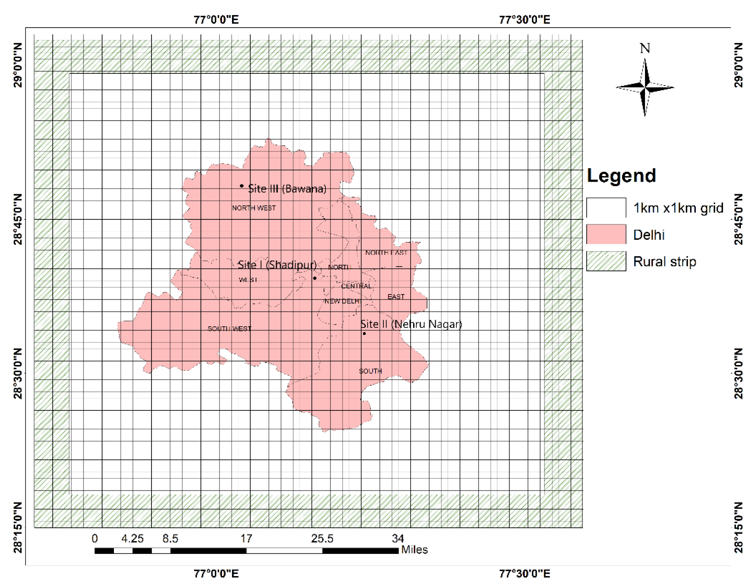
2.1. Study Area

Delhi is situated on the banks of river Yamuna at a latitude of 28.38° N and a longitude of 77.17° E (Figure 1). It spreads over 1483 sq km, and its population is 16.8 million, with a density of 11,320 persons per sq km [39]. It has nine districts: North, North West, North East, South, South West, East, West, Central, and New Delhi. These districts are highly populous, with a large number of residential and commercial buildings. Delhi has a subtropical climate, with an average annual maximum temperature of 31.4 °C and an average annual minimum temperature of 19 °C [40]. It is characterized by extreme dryness, with intensely hot summers and cold winters. Delhi receives an annual rainfall of around 79.8 cm, and relative humidity varies from 39% to 66% in monsoon season [40].

2.2. LULC Mapping

In the present study, we used cloud-free Sentinel 2A Multispectral Imager data from March 2018 for LULC mapping of Delhi. Sentinel 2 is an Earth Observation mission developed and operated by the European Space Agency. It consists of two sun-synchronous polar-orbiting satellites at a phase of 180° to each other. The two satellites measure radiances in 13 spectral bands varying from 443 nm to 2190 nm to monitor land surface conditions at a spatial resolution ranging from 10m to 60m with a swath width of 290 km. The multispectral instrument provides data for land cover, atmospheric correction, and cloud/snow separation. Two scenes of S-2A Level-1C with radiometric and geometric corrections were acquired for this study. Four bands (i.e., B-2, B-3, B-4, and B-8) with a spatial resolution of 10 m were used for LULC mapping in our study. The unsupervised classification was used to classify the image into clusters using the isodata algorithm [41,42]. These clusters were then supervised and grouped into five classes of LULC, namely water body, vegetation, built-up, rocky terrain and open land [43,44,45]. The accuracy assessment was performed using the dedicated tool in ERDAS IMAGINE software, which produces a confusion matrix (or error matrix) and Kappa statistics of the assessment. Furthermore, to get the percentage of LULC belonging to different classes in each grid cell, a grid with a cell size of 1km x 1km was overlaid on the classified LULC image, and the zonal analysis was performed.

2.3. MODIS LST Data

The Moderate Resolution Imaging Spectroradiometer (MODIS) instrument aboard the Terra and Aqua Satellites of NASA’s Earth Observing System (EOS) Mission measures radiances (12-bit data) in 36 bands, covering the spectral range from 0.405 to 14.385 µm, at spatial resolutions of 250 (2 bands), 500 (5 bands) and 1000 m (29 bands). The satellites orbit the Earth in sun-synchronous, near-polar circular orbits with equator crossing times of 10.30 a.m./p.m. (Terra), and 1.30 p.m./a.m. (Aqua). With a swath width of 2330 km, the instrument views the entire Earth’s surface every 1-2 days [46].

To gain an insight into the UHI formation over Delhi and its association with LULC, we used the MODIS Aqua product MYD11A2.v006 to obtain the LST (1 km resolution) data over Delhi for March 2018. MYD11A2.v006 is an 8-day composite, a simple average product derived from the MYD11A1 daily global product [47]. For the estimation of UHII, we used monthly average LST (MYD11A2.v006) of each site and its surrounding rural areas near Delhi (Figure 1) for the period from January 2018 to December 2018. UHII for each site was calculated by subtracting the average LST (LST_rural) of rural areas (rural strip) from average LST over given sites (LST_s) in Delhi [28]. Thus, monthly UHII for given sites (I, II and III) was calculated with Equation (1):

$${\mathrm{UHII}}_{\mathrm{s}}={\mathrm{LST}}_{\mathrm{s}}-{\mathrm{LST}}_{\mathrm{rural}}$$

(1)

The same grid with a cell size of 1km x1km used earlier on the LULC map was also overlaid on the LST map for statistical analysis. Correlation and linear regression analysis were performed with the percentage of LULC and nighttime LST [28].

Furthermore, to examine the correlation between LST and air temperature, MODIS Aqua (MYD11A2.v006), and Terra (MOD11A2.v006) day and night monthly average products for the period from January 2018 to December 2018 were used.

2.4. Building Simulation

To estimate the impact of LULC on surface temperature (both land and air) and energy consumption, we performed a simulation using a calibrated building model [48]. Energy simulations were performed on the calibrated building model using Design Builder (60.0.10.019) software, which uses Energy Plus as a simulation engine. Monthly total energy and cooling electricity consumption were calculated.

For the purpose of simulation, we identified three different sites based on their LST values, UHII, availability of hourly air temperature data, and the percentage of LULC classes for these sites. Site-I (i.e., Shadipur) represents a typical dense urban built-up site (93% built-up area) in Delhi witnessing the UHI effect, with relatively high average annual nighttime LST valueof 293.5 K, with a UHII intensity ranging from 0.9 K to 5.9 K. On the other hand, Site-III (Bawana) represents a typical rural site with abundant vegetation (~54%) in Delhi, experiencing minimal UHI effect and relatively low average annual nighttime LST values of 290 K, with UHII varying from 0.0 K to 0.4 K. Site-II (Nehru Nagar) represents a relatively less dense urban site (65% built-up area) with more green and open land (6%), witnessing a moderate UHI effect with average annual nighttime LST values of 291 K and a UHII intensity between 0.1K and 5 K.

2.4.1. Calibrated Building

The calibrated building we used in this analysis is a learning center named “Satyam Learning Centre” (Figure 2). The building has cabins, a library, pantry, toilets, electrical and utility rooms. The structure consists of two floors and no basement and is divided into an east and west wing. For the study, we used the west wing of the top floor, which is fitted with separate energy meters for equipment, lighting, cooling, and other end-uses. A brief description of the building envelope is given in

Table 1. Heat transfer coefficient and thermal conductivity of the building envelope.

Type of Building Envelope	Material Description	Heat Transfer Coefficient (U-value)	Thermal Conductivity (k-value)
External Wall	228 mm brick with mortar plaster on both sides	1.62 Wm−2K	0.840 Wm−1K for brick and 0.88 Wm−1K for mortar plaster
Internal Wall	190 mm brick with gypsum plaster on both sides	2.0 Wm−2K	0.840 Wm−1K for brick and 0.18 Wm−1K−1for gypsum plaster
Grey Roof	101.60 mm concrete slab with 20.30 mm plaster on the upper side and expanded polystyrene thermocol for roof insulation. An air gap of 0.9 m is provided in the ceiling made of a plasterboard	0.618 Wm−2K and an absorptance of 0.7 Wm−2K	1.35 Wm−1K for roof slab and 0.046 Wm−1K−1 for expanded polystyrene

.

Other details of the building model are given below:

• Window glazing: It occupies 7% of the external wall area with a U-value of 5.778 Wm⁻²K⁻¹;
• The heating ventilation air conditioning (HVAC) System: The HVAC system is a direct expansion air conditioning unit (DX system) covering the total conditioned area of 663 m²;
• Power density: 9.9 (W/m²) for general lighting, 11 (W/m²) for computer appliances, 1.18 (W/m²) for office equipment has been used;
• Occupancy: The total occupancy is 61, including students and an instructor. This has been derived by taking into account the number of available seats.

2.4.2. Weather Files

The weather file provided by the Indian Society of Heating, Refrigerating, and Air Conditioning Engineers (ISHRAE) of New Delhi was modified for building simulation. In the modified weather files for each site, we replaced the hourly dry bulb temperature with one year (2018) corresponding ground station air temperature data provided by the Central Pollution Control Board of Delhi.

3. Result and Discussion

3.1. Urban heat Island Intensity (UHII) Analysis

The monthly variation of UHII over Delhi during night time is depicted in Figure 3 for the period from January 2018 to December 2018. It may be observed that UHII remains positive throughout the year. Higher UHII was found over Shadipur (5–6 K) and Nehru Nagar (4–5 K) during March and April, and a lower UHII (0.9–1 K) was observed during monsoon season in July and August. Lower UHII during monsoon season is mainly because the difference in radiation loss efficiencies between urban and rural areas is suppressed by cloudy skies. Among the three sites, the lowest UHII values throughout the year were seen over Bawana, as it is a predominantly rural site.

3.2. Land Use and Land Cover and UHI Pattern

LULC-classified images are significant for decision makers and urban planners to determine the dynamics of urban growth. Multispectral imagery is the main source by which changes in LULC patterns are studied. Through LULC mapping, we were able to examine the association of LST with LULC. Figure 4a shows the classified image of Delhi and its surrounding area, obtained from the Sentinel-2 Earth Observation Satellite. The most prominent class is vegetation, which comprises of mostly agriculture land, covering ~ 53% of the total area. This class is mainly prevalent in the surrounding rural region of Delhi and in the northwest and southwest districts of Delhi. It is observed that the built-up area is the second most prominent class, covering 34% of the total area, and it is more prevalent over the Delhi region. This is due to the high density of residential and commercial buildings, which cater to the needs of a large population in the capital. The other LULC classes consist of open land (8%), rocky terrain (5%), and water body (1%). An accuracy assessment resulted in 92% overall classification accuracy based on random points and a Kappa coefficient of 0.90 (Appendix A

Table A1. Overall accuracy assessment of LULC for the month of March.

Class Name	Reference Totals	Classified Totals	Number Correct	Producers Accuracy	Users Accuracy
Water Body	3	3	3	100.00%	100.00%
Rocky Terrain	18	18	16	88.89%	88.89%
Built up Area	23	21	19	82.61%	90.48%
Open Land	17	19	17	100.00%	89.47%
Vegetation	29	29	27	93.10%	93.10%

and

Table A2. Kappa statistics report.

Class Name	Kappa
Water Body	1
Rocky terrain	0.8645
Built up Area	0.8763
Open Land	0.8732
Vegetation	0.9029

). To gain an insight into how the three sites differ from each other, the LULC percentage in a 1km x 1km grid for each site was calculated (

Table 2. Percentage of land use and land cover (LULC) classes in 1 km × 1 km grid of simulation sites.

Sites	VEGETATION 1 km × 1 km	WATER_BODY 1 km × 1 km	OPEN_LAND 1 km × 1 km	ROCKY_TERRAIN 1 km × 1 km	BUILT_UP_AREA 1 km × 1 km
Site-I (Shadipur)	5%	1%	2%	0%	93%
Site-II (Nehru Nagar)	27%	3%	6%	0%	65%
Site-III (Bawana)	54%	2%	5%	0%	38%

). It indicates that Site-I and Site-II show a higher percentage of built-up areas (93% and 65%, respectively), while a smaller built-up area (38%) was observed at Site-III. Furthermore, it was found that Site-III shows a higher proportion of vegetation (~54%) than the remaining two sites (5% at site-I and 27% at Site-II).

Figure 4b reveals the nocturnal heat island formation over Delhi in the month of March. It is observed that higher values of LST are found in the central parts of Delhi where Site-I (Shadipur) is situated, while lower LST values were observed in the peripheral regions of the northwest (where Site-III, i.e., Bawana is situated) and southwest districts of Delhi.

A comparative examination of Figure 4a,b reveals that regions with higher proportions of built-up areas also have higher LST. This is clearly visible over the central parts of the city. It is pertinent to mention here that almost every district has some proportion of built-up area, which, in turn, has higher LST values. The outskirts of the city in the northwest and southwest districts show a large amount of vegetation (agricultural land). This region also has a significantly lower density of built-up areas, which has resulted in the lower LST in this region. Su et al. [49] examined the relationship between LULC classes and LST, and also found higher LSTs in the densely built-up areas compared to vegetative areas.

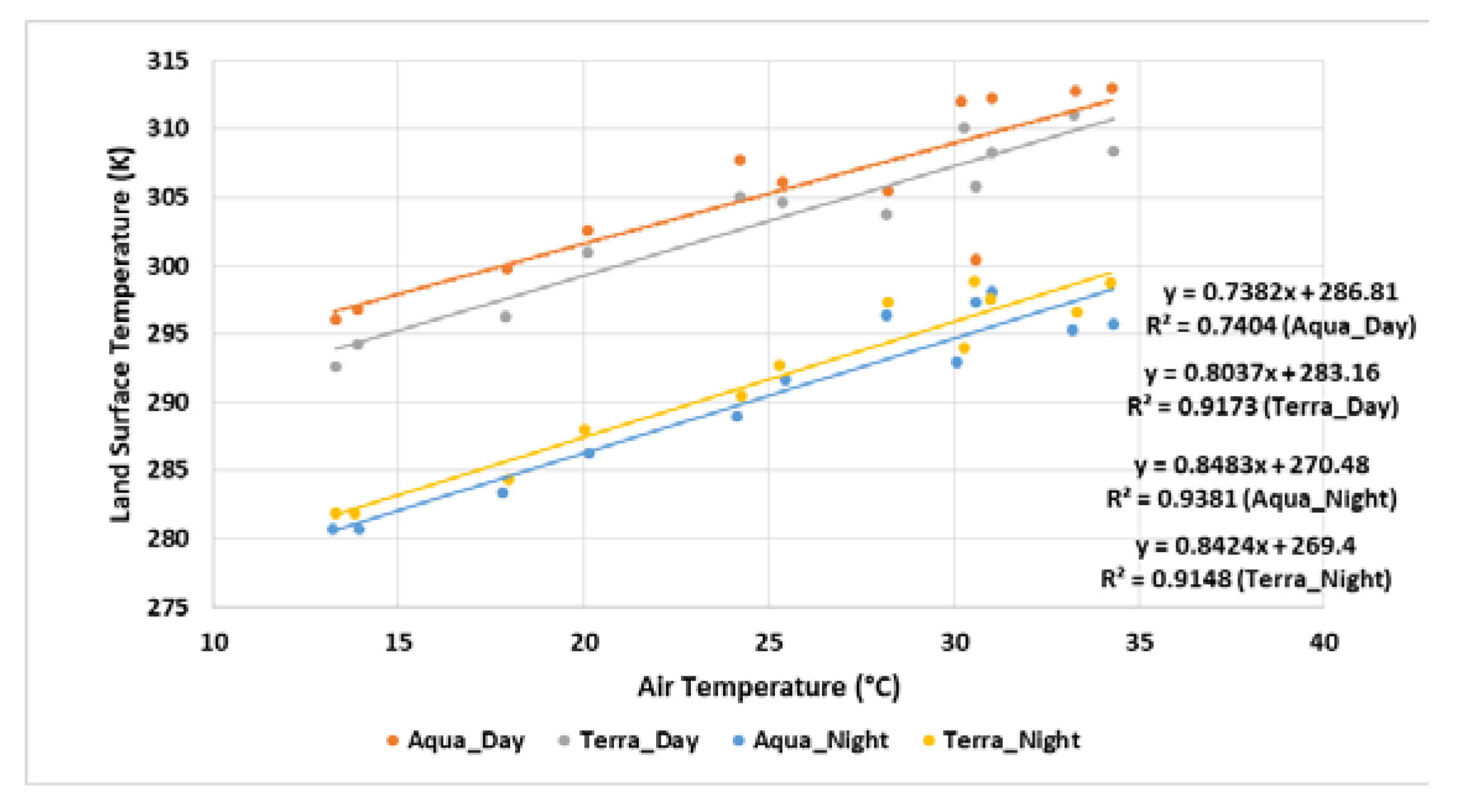
3.3. Statistical Analysis

The correlation between nighttime LST and LULC percentage on the basis of the 1 km × 1 km grid analysis is shown in

Table 3. Correlation matrix between nighttime land surface temperature (LST) and land use and land cover variables.

		Vegetation	Water Body	Open Land	Rocky Terrain	Built-up Area	Nighttime LST
Vegetation	Pearson Correlation	1	−0.100 **	−0.445 **	−0.328 **	−0.797 **	−0.713 **
	Sig. (2-tailed)		0.000	0.000	0.000	0.000	0.000
Water body	Pearson Correlation	−0.100 **	1	−0.001	−0.034 **	0.023	0.091 **
	Sig. (2-tailed)	0.000		0.930	0.005	0.055	0.000
Open land	Pearson Correlation	−0.445 **	−0.001	1	−0.127 **	0.380 **	0.196 **
	Sig. (2-tailed)	0.000	0.930		0.000	0.000	0.000
Rocky terrain	Pearson Correlation	−0.328 **	−0.034 **	−0.127 **	1	−0.156 **	0.300 **
	Sig. (2-tailed)	0.000	0.005	0.000		0.000	0.000
Built-up area	Pearson Correlation	−0.797 **	0.023	0.380 **	−0.156 **	1	0.657 **
	Sig. (2-tailed)	0.000	0.055	0.000	0.000		0.000
Nighttime LST	Pearson Correlation	−0.713 **	0.091 **	0.196 **	0.300 **	0.657 **	1
	Sig. (2-tailed)	0.000	0.000	0.000	0.000	0.000

**. Correlation is significant at the 0.01 level (2-tailed).

. It is observed that a strong positive correlation exists between nighttime LST and built-up areas. A large amount of heat absorbed during daytime is slowly re-radiated at nighttime in urban areas due to large concrete surfaces and structures [5]. On the other hand, vegetation cover is found to be negatively correlated with nighttime LST, which indicates that areas with high vegetation cover have lower LST.

A regression analysis (

Table 4. Results of regression analysis.

Model Description	Dependent Variable	Explanatory Variable	B	Std. Error	t-value	Sig. Level	Adjusted R Square
Linear regression model for Nighttime LST	Nighttime LST_	Constant	289.115	0.088	3270.879	0.000	0.55
		Built-up area	0.021	0.001	19.565	0.000
		Vegetation	−0.040	0.001	−41.796	0.000
		Open land	−0.047	0.003	−17.777	0.000
		Water body	0.017	0.005	3.389	0.001

) shows that built-up areas and water bodies have positive regression coefficients, which suggest that these variables have a positive influence on nighttime LST. In contrast, vegetation and open land show negative regression coefficients in the nighttime LST model, which suggests that vegetation and open land contribute to a decrease in the nighttime LST. Furthermore, the adjusted R² value observed for the model is 0.55, which shows that LULC variables play a major role in explaining nighttime UHII over Delhi.

3.4. Association Between Urban Heat Island and Building Consumption

Furthermore, we examined the association of electricity consumption and cooling load with the urban heat island effect. We chose three sites, viz Site-I (Shadipur), Site-II (Nehru Nagar), and Site-III (Bawana) representing locations with different UHII and annual LST values. For all three sites, hourly air temperature data was available. Figure 5 depicts the correlation between LST and air temperature at Shadipur. A good correlation between the two (R² varying from 0.74 to 0.93) indicates that LST can be effectively used to predict or represent air temperature over the location. Thus, it is reasonable to expect that the variations in the UHI effect at the three sites are not just reflected in terms of differences in LST, but also in terms of differences in air temperatures.

Figure 6 shows the monthly average air temperature variation at the three sites. Minimum temperatures are observed in December and January, while maximum temperatures are observed in June. Furthermore, it is observed that Site-I (Shadipur), which is located in the central part of Delhi, has the highest average air temperatures among the three sites almost throughout the year. In contrast, Site-III (Bawana), which is located in the rural area of Delhi, has the least average air temperature among the three sites. Thus, the difference in annual LST and monthly UHII at the three sites is also reflected in air temperature at the three sites throughout the year. It is also observed that the air temperature difference among the three sites is the least during the monsoon months. This is expected since the cloud cover in monsoon months suppresses the differential radiation loss efficiency between the urban and rural areas.

Using the calibrated building model, we performed simulations to estimate the energy consumption by the calibrated building placed at the three sites. Figure 7 shows the monthly consumption pattern of the building model at the three sites. Consumption trends at all sites are similar, i.e., higher values for summer and the monsoon season (April to July) and lower values for the winter season (December and January). Furthermore, it is observed that Site-I (Shadipur) shows the highest electricity consumption among the three sites, while Site-III (Bawana) shows the least electricity consumption, almost throughout the year. During the monsoon months, when the air temperature difference among the three sites is the least, the difference in their electricity consumption is also the least. When comparing the three sites (

Table 5. Simulation sites and annual electricity consumption and cooling electricity consumption details.

Sites	Location	Annual UHII (K)		Average Annual UHI (K)	Annual Electricity Consumption (MWh/y)	Annual Cooling electricity consumption(MWh/y)
		Minimum	Maximum
Site-I	Shadipur (28.6510° N, 77.1562° E)	0.9	5.9	293.5	255.21	143.82
Site-II	Nehru Nagar 28.5706° N, 77.2506° E	0.1	50.0	292.1	243.49	132.10
Site-III	Bawana (28.7932° N, 770.0483° E	0.0	0.4	290.02	235.69	124.30

), we observed the highest annual electricity consumption (255.21 MWh/y) at the location with high surface (land and air) temperatures, i.e., Site-I. However, annual consumption was lower for the other two sites with lower annual LSTs, i.e., 243.49 MWh/y for Site-II and 235.69 MWh/y for Site-III. This is because a major part of electricity consumption comes from the use of cooling appliances for thermal comfort in summers and during the monsoon season.

The monthly cooling electricity consumption at the three sites is shown in Figure 8. It is seen that cooling electricity consumption is higher for the summer and monsoon months and is lowest for the winter months. The annual cooling electricity corresponds to 143.82 MWh/y, 132.10 MWh/y, and 124.30 MWh/y for Sites I, II, and III, respectively. This observation suggests that buildings in locations with higher UHII and higher LSTrequire higher cooling loads and vice versa. Between Site-I and III, there is a difference of 19.52 MWh/y for annual electricity consumption and 19.52 MWh/y for cooling energy consumption. This is the approximate amount of energy that can be saved by a typical building with specifications similar to the calibrated building model if UHI mitigation measures are implemented effectively. Niachou et al. [50] reported the annual energy-saving potential of green roofs as 37–48% in non-insulated buildings, 4–7% in moderately insulated buildings and 2% in well-insulated buildings in Athens, Greece. Similarly, Bhatia et al. [48] observed that by implementing cool roof measures on the building, energy savings between 3.16% and 4.88% could be achieved in different climatic conditions in India. As per the census of India 2011 [39], there are 3,435,999 households in Delhi. If each household were to apply effective UHI mitigation strategies, a large amount of energy could be saved annually in the city of Delhi.

4. Limitations

The present study has been conducted by simulating the electricity consumption of the calibrated building model placed in three different thermal regimes in Delhi. However, buildings in real life situations may be very different from the calibrated building model used in this study. Thus, the results of this study cannot be applied to estimate the total excess electricity consumption for the entire city of Delhi. Furthermore, the information on building parameters and other variables required in the model is hardly available for all the buildings and sites in the city. Therefore, we were constrained by the use of the calibrated building model to demonstrate the impact of urban heat island on electricity consumption in a typical building.

5. Conclusions

In this paper, we showed that LULC changes brought about by urbanization cause the formation of a nighttime urban heat island over the dense built-up areas almost throughout the year, with varying intensity. We found that built-up areas, vegetation cover and open land are the three most important variables governing the nighttime LST over Delhi and its surrounding areas. While built-up areas are found to have a positive influence over LST, vegetation and open land are observed to have negative influence over LST. Sites situated at different locations showed different UHI intensity, with Site-I (Shadipur) showing the highest UHI intensity and Site-III (Bawana), located in the rural area of Delhi, showing the least UHI intensity among the three sites. These differences were also witnessed in monthly average air temperatures over the three sites.

Energy simulation performed over the three sites using a calibrated building model showed that annual electricity consumption is significantly influenced by surface temperature variations brought about by urbanization. Site-I exhibited a higher annual electricity consumption, while Site-III showed a lower electricity consumption. We find that annual energy consumption in the calibrated building at Site-I was higher by about 19.52 MWh/y compared to Site-III. The study suggests that a large amount of energy could be saved in Delhi if UHI mitigation measures such as cool roofs and green roofs are adopted. If such measures are applied to other Indian cities witnessing urban heat island formation, the amount of energy saved in the Indian context would be quite significant.

References

1. Roth, M.; Oke, T.R.; Emery, W.J. Satellite-derived urban heat islands from three coastal cities and the utilization of such data in urban climatology. Int. J. Remote Sens. 1989, 10, 1699–1720. [Google Scholar] [CrossRef]
2. Oke, T.R. The Heat Island of the Urban Boundary Layer: Characteristics, Causes and Effects. Wind Clim. Cities 1995, 81–107. [Google Scholar] [CrossRef]
3. Priyadarsini, R. Urban heat island and its impact on building energy consumption. Adv. Build. Energy Res. 2009, 3, 261–270. [Google Scholar] [CrossRef]
4. Oke, T.R. Canyon geometry and nocturnal urban heat island: Comparison of scale model and field observations. J. Climatol. 1981, 1, 237–254. [Google Scholar] [CrossRef]
5. Rizwan, A.; Dennis, L.; Liu, C. A review on the generation, determination and mitigation of Urban Heat Island. J. Environ. Sci. 2008, 20, 120–128. [Google Scholar] [CrossRef]
6. Landsberg, H.E. Man-made climatic changes. Science (80-) 1970, 170, 1265–1274. [Google Scholar] [CrossRef]
7. Santamouris, M.; Paraponiaris, K.; Mihalakakou, G. Estimating the ecological footprint of the heat island effect over Athens, Greece. Clim. Chang. 2007, 80, 265–276. [Google Scholar] [CrossRef]
8. Mylona, E.; Daskalopoulou, V.; Sykioti, O.; Koutroumbas, K.; Rontogiannis, A. Classification of Sentinel-2 Images Utilizing Abundance Representation. Proceedings 2018, 2, 328. [Google Scholar] [CrossRef] [Green Version]
9. Park, H. Features of the island in Seoul and its surrounding cities. Atmos. Environ. 1986, 20, 1859–1866. [Google Scholar] [CrossRef]
10. Hart, M.A.; Sailor, D.J. Quantifying the influence of land-use and surface characteristics on spatial variability in the urban heat island. Theor. Appl. Climatol. 2009, 95, 397–406. [Google Scholar] [CrossRef]
11. Kohler, M.; Blond, N.; Clappier, A. A city scale degree-day method to assess building space heating energy demands in Strasbourg Eurometropolis (France). Appl. Energy 2016, 184, 40–54. [Google Scholar] [CrossRef]
12. Voogt, J.A.; Oke, T.R. Thermal remote sensing of urban climates. Remote Sens. Environ. 2003, 86, 370–384. [Google Scholar] [CrossRef]
13. Feizizadeh, B.; Blaschke, T. Examining Urban Heat Island Relations to Land Use and Air Pollution: Multiple Endmember Spectral Mixture Analysis for Thermal Remote Sensing. IEEE J. Sel. Top. Appl. Earth Obs Remote Sens. 2013, 6, 1749–1756. [Google Scholar] [CrossRef]
14. Cheval, S.; Dumitrescu, A. The July urban heat island of Bucharest as derived from modis images. Theor. Appl. Clim. 2009, 145–153. [Google Scholar] [CrossRef]
15. Keramitsoglou, I.; Kiranoudis, C.T.; Ceriola, G.; Weng, Q.; Rajasekar, U. Identification and analysis of urban surface temperature patterns in Greater Athens, Greece, using MODIS imagery. Remote Sens. Environ. 2011, 115, 3080–3090. [Google Scholar] [CrossRef]
16. Liu, L.; Zhang, Y. Urban heat island analysis using the landsat TM data and ASTER Data: A case study in Hong Kong. Remote Sens. 2011, 3, 1535–1552. [Google Scholar] [CrossRef] [Green Version]
17. Estoque, R.C.; Murayama, Y. Monitoring surface urban heat island formation in a tropical mountain city using Landsat data (1987–2015). ISPRS J. Photogramm. Remote Sens. 2017, 133, 18–29. [Google Scholar] [CrossRef]
18. Zhou, J.; Li, J.; Yue, J. Analysis of urban heat Island (UHI) in the Beijing meteropolitan area by time series MODIS data. In Proceedings of the 2010 IEEE International Geoscience and Remote Sensing Symposium, Honolulu, HI, USA, 25–30 July 2010; pp. 3327–3330. [Google Scholar]
19. Anniballe, R.; Bonafoni, S.; Pichierri, M. Spatial and temporal trends of the surface and air heat island over Milan using MODIS data. Remote Sens. Environ. 2014, 150, 163–171. [Google Scholar] [CrossRef]
20. Chen, X.L.; Zhao, H.M.; Li, P.X.; Yin, Z.Y. Remote sensing image-based analysis of the relationship between urban heat island and land use/cover changes. Remote Sens. Environ. 2006, 104, 133–146. [Google Scholar] [CrossRef]
21. Streutker, D.R. A remote sensing study of the urban heat island of Houston, Texas. Int. J. Remote Sens. 2002, 23, 2595–2608. [Google Scholar] [CrossRef]
22. Sekertekin, A.; Kutoglu, S.H.; Kaya, S. Evaluation of spatio-temporal variability in Land Surface Temperature: A case study of Zonguldak, Turkey. Environ. Monit. Assess 2016, 188, 1–15. [Google Scholar] [CrossRef] [PubMed]
23. Streutker, D.R. Satellite-measured growth of the urban heat island of Houston, Texas. Remote Sens. Environ. 2003, 85, 282–289. [Google Scholar] [CrossRef]
24. Kato, S.; Yamaguchi, Y. Analysis of urban heat-island effect using ASTER and ETM+ Data: Separation of anthropogenic heat discharge and natural heat radiation from sensible heat flux. Remote Sens. Environ. 2005, 99, 44–54. [Google Scholar] [CrossRef]
25. Fabrizi, R.; Bonafoni, S.; Biondi, R. Satellite and ground-based sensors for the Urban Heat Island analysis in the city of Rome. Remote Sens. 2010, 2, 1400–1415. [Google Scholar] [CrossRef] [Green Version]
26. Hirano, Y.; Fujita, T. Evaluation of the impact of the urban heat island on residential and commercial energy consumption in Tokyo. Energy 2012, 37, 371–383. [Google Scholar] [CrossRef]
27. Kolokotroni, M.; Zhang, Y.; Watkins, R. The London heat island and building cooling design. Sol. Energy 2005, 81, 743–748. [Google Scholar] [CrossRef] [Green Version]
28. Pandey, A.K.; Singh, S.; Berwal, S.; Kumar, D.; Pandey, P.; Prakash, A.; Lodhi, N.; Maithani, S.; Jain, V.K.; Kumar, K. Spatio—temporal variations of urban heat island over Delhi. Urban Clim. 2014, 10, 119–133. [Google Scholar] [CrossRef]
29. Yang, P.; Ren, G.Y.; Liu, W.D. Spatial and Temporal Characteristics of Beijing Urban Heat Island Intensity. J. Appl. Meteorol. Climatol. 2013, 52, 1803–1816. [Google Scholar] [CrossRef]
30. Li, X.; Zhou, Y.; Yu, S.; Jia, G.; Li, H.; Li, W. Urban heat island impacts on building energy consumption: A review of approaches and findings. Energy 2019. [Google Scholar] [CrossRef]
31. Hwang, R.L.; Lin, C.Y.; Huang, K.T. Spatial and temporal analysis of urban heat island and global warming on residential thermal comfort and cooling energy in Taiwan. Energy Build. 2017, 152, 804–812. [Google Scholar] [CrossRef]
32. Santamouris, M.; Papanikolaou, N.; Livada, I.; Koronakis, I.; Georgakis, C.; Argiriou, A.; Assimakopoulos, D.N. On the impact of urban climate on the energy consuption of building. Sol. Energy 2001, 70, 201–216. [Google Scholar] [CrossRef]
33. Salvati, A.; Coch Roura, H.; Cecere, C. Assessing the urban heat island and its energy impact on residential buildings in Mediterranean climate: Barcelona case study. Energy Build. 2017, 146, 38–54. [Google Scholar] [CrossRef] [Green Version]
34. Rahman, A.; Kumar, Y.; Fazal, S.; Bhaskaran, S. Urbanization and Quality of Urban Environment Using Remote Sensing and GIS Techniques in East Delhi-India. J. Geogr. Inf. Syst. 2011, 3, 61–83. [Google Scholar] [CrossRef] [Green Version]
35. Sharma, R.; Joshi, P.K. Monitoring Urban Landscape Dynamics Over Delhi (India) Using Remote Sensing (1998-2011) Inputs. J. Indian Soc. Remote Sens. 2013, 41, 641–650. [Google Scholar] [CrossRef]
36. Pandey, P.; Kumar, D.; Prakash, A.; Masih, J.; Singh, M.; Kumar, S.; Jain, V.K.; Kumar, K. A study of urban heat island and its association with particulate matter during winter months over Delhi. Sci. Total. Environ. 2012, 414, 494–507. [Google Scholar] [CrossRef] [PubMed]
37. Ramesh, S.; Natarajan, B.; Bhagat, G. Peak load prediction using weather Variables. Energy 1988, 13, 671–679. [Google Scholar] [CrossRef]
38. Gupta, E. Global warming and electricity demand in the rapidly growing city of Delhi: A semi-parametric variable coefficient approach. Energy Econ. 2012, 34, 1407–1421. [Google Scholar] [CrossRef] [Green Version]
39. Chandramouli, C. Census of India 2011, Primary Census Abstract; Office of the Registrar General & Census Commissioner: New Delhi, India, 2012.
40. India Meteorological Department (Ministry of Earth Sciences) Home Page 2014. Available online: https://mausam.imd.gov.in/imd_latest/contents/index_smart_cities1.php (accessed on 10 March 2020).
41. Ball, G.H.; Hall, D.J. Isodata, a Novel Method of Data Analysis and Pattern Classification. In Clearinghouse for Federal Scientific &Technical Information Springfield; Stanford Research Institute: Menlo Park, CA, USA, 1965. [Google Scholar]
42. Zhong, Y.; Zhang, L.; Huang, B.; Li, P. An unsupervised artificial immune classifier for multi/hyperspectral remote sensing imagery. IEEE Trans. Geosci. Remote Sens. 2006, 44, 420–431. [Google Scholar] [CrossRef]
43. Fukue, K.; Shimoda, H.; Matumae, Y.; Yamaguchi, R.; Sakata, T. Evaluations of unsupervised methods for land-cover/use classifications of landsat TM data. Geocarto Int. 1988, 3, 37–44. [Google Scholar] [CrossRef]
44. Babykalpana, Y.; ThanushKodi, D.K. Supervised/Unsupervised Classification of LULC Using Remotely Sensed data for Coimbatore city, India. Int. J. Comput. Appl. 2010, 2, 26–30. [Google Scholar] [CrossRef]
45. Al-Tamimi, S.; Al-Bakri, J.T. Comparison Between Supervised and Unsupervised Classifications for Mapping Land Use/Cover in Ajloun Area. Jordan J. Agric. Sci. 2005, 1, 73–83. [Google Scholar]
46. Justice, C.O.; Vermote, E.; Townshend, J.R.; Defries, R.; Roy, D.P.; Hall, D.K.; Salomonson, V.V.; Privette, J.L.; Riggs, G.; Strahler, A.; et al. The Moderate Resolution Imaging Spectroradiometer (MODIS): Land Remote Sensing for Global Change Research. IEEE Trans. Geosci. Remote Sens. 1998, 36, 1228–1249. [Google Scholar] [CrossRef] [Green Version]
47. Land processes distribute active archive center (LP DAAC) Home Page. Available online: https://lpdaac.usgs.gov/products/ (accessed on 10 March 2020).
48. Bhatia, A.; Mathur, J.; Garg, V. Calibrated simulation for estimating energy savings by the use of cool roof in five Indian climatic zones. J. Renew. Sustain. Energy 2011, 3. [Google Scholar] [CrossRef]
49. Su, W.; Gu, C.; Yang, G. Assessing the Impact of Land Use/Land Cover on Urban Heat Island Pattern in Nanjing City, China. J. Urban Plan. Dev. 2011, 136, 365–373. [Google Scholar] [CrossRef]
50. Niachou, A.; Papakonstantinou, K.; Santamouris, M.; Tsangrassoulis, A.; Mihalakakou, G. Analysis of the green roof thermal properties and investigation of its energy performance. Energy Build. 2001, 33, 719–729. [Google Scholar] [CrossRef]
Figure 1. Study area: Delhi.
Climate 08 00071 g001
Figure 2. Calibrated building model.
Climate 08 00071 g002
Figure 3. Monthly variation of surface heat island intensity over Delhi for the period of January 2018 – December 2018.
Climate 08 00071 g003
Figure 4. Land use land cover (a) and land surface temperature (b) map of Delhi (8 March 2018).
Climate 08 00071 g004
Figure 5. The correlation between air temperature and land surface temperature for the Shadipur site (Site-I).
Climate 08 00071 g005
Figure 6. Monthly average air temperature pattern over three sites of Delhi.
Climate 08 00071 g006
Figure 7. Total electricity consumption of building in three different thermal regimes of LST of Delhi.
Climate 08 00071 g007
Figure 8. Cooling electricity consumption of building in three different thermal regimes of LST of Delhi.
Climate 08 00071 g008