Instrumental and Observational Problems of the Earliest Temperature Records in Italy: A Methodology for Data Recovery and Correction

Abstract

A distinction is made between data rescue (i.e., copying, digitizing, and archiving) and data recovery that implies deciphering, interpreting, and transforming early instrumental readings and their metadata to obtain high-quality datasets in modern units. This requires a multidisciplinary approach that includes: palaeography and knowledge of Latin and other languages to read the handwritten logs and additional documents; history of science to interpret the original text, data, and metadata within the cultural frame of the 17th, 18th, and early 19th centuries; physics and technology to recognize bias of early instruments or calibrations, or to correct for observational bias; and astronomy to calculate and transform the original time in canonical hours that started from twilight. The liquid-in-glass thermometer was invented in 1641 and the earliest temperature records started in 1654. Since then, different types of thermometers have been invented, based on the thermal expansion of air or selected thermometric liquids with deviation from linearity. Reference points, thermometric scales, and calibration methodologies were not comparable, and not always adequately described. Thermometers had various locations and exposures, e.g., indoor, outdoor, on windows, gardens or roofs, facing different directions. Readings were made only one or a few times a day, not necessarily respecting a precise time schedule: this bias is analysed for the most popular combinations of reading times. The time was based on sundials and local Sun, but the hours were counted starting from twilight. In 1789–1790, Italy changed system and all cities counted hours from their lower culmination (i.e., local midnight), so that every city had its local time; in 1866, all the Italian cities followed the local time of Rome; in 1893, the whole of Italy adopted the present-day system, based on the Coordinated Universal Time and the time zones. In 1873, when the International Meteorological Committee (IMC) was founded, later transformed into the World Meteorological Organization (WMO), a standardization of instruments and observational protocols was established, and all data became fully comparable. In dealing with the early instrumental period, from 1654 to 1873, the comparison, correction, and homogenization of records is quite difficult, mainly because of the scarcity or even absence of metadata. This paper deals with this confused situation, discussing the main problems, but also the methodologies to recognize missing metadata, distinguish indoor from outdoor readings, correct and transform early datasets in unknown or arbitrary units into modern units, and, finally, in which cases it is possible to reach the quality level required by the WMO. The aim is to explain the methodology needed to recover early instrumental records, i.e., the operations that should be performed to decipher, interpret, correct, and transform the original raw data into a high-quality dataset of temperature, usable for climate studies.

1. Introduction

Data rescue (DARE) is the process of securing data at risk of being lost due to deterioration, obsolescence of the storage media, or other factors, and ensuring that data are freely available to the scientific community [1]. DARE consists of archiving and imaging paper records, copying and digitizing data, and updating digital records and supports. This is an ongoing task of World Meteorological Organization (WMO), Copernicus, ECMWF, National Meteorological and Hydrological Services, and other institutions. Guidelines on DARE have been published by WMO [1]. DARE activity has been documented by a number of authors focused on partial or global inventories [2,3,4,5,6,7,8]. In Europe, most rescued data and metadata are after 1850 [9], although there is an effort to gather records pre-1850 [10].

In the pioneering period (i.e., from 1641 when the liquid-in-glass thermometer was invented, or 1654 when the earliest records were performed, to 1873), every observer was free to invent, build, and use instruments, individual methods, and protocols. Some international networks, like the one established by the Grand Duke of Tuscany Ferdinand II de’ Medici (active 1654–1670), the Royal Society, London (active 1724–1735), and the Societas Meteorologica Palatina, Mannheim (active 1781–1792), contributed to homogenizing instruments and practices. In the early period, thermometers differed in measuring principles, linear or non-linear responses of thermometric fluids, calibration methods, location and exposure (including indoor or outdoor use), reading times, and adoption or non-adoption of shields or screens against rain and/or solar radiation. As a result, data changed from observer to observer, and caused records to be hardly comparable between them, or even difficult to interpret.

Another problem of that period is the lack of metadata, because observers thought that the focus was on the result, i.e., the observed values, and these had to be accepted due to the scientific authority of the author, who did not lend himself easily to being criticized or revealing his secrets. Furthermore, anything that seemed obvious or irrelevant to the observer was not mentioned. In most cases, registers of observations, and publications reported plenty of data but missed the metadata necessary to interpret them.

A turning point for meteorology was the International Meteorological Congress held in Leipzig [11], St Petersburg, and Vienna [12], in 1873, when the International Meteorological Committee (IMC) was founded as a forum for exchanging weather data and research. This initiative was followed by a series of IMC meetings, e.g., Rome in 1879 [13], Berne in 1880 [14], Copenhagen in 1882 [15], Paris in 1885 [16], Zürich in 1888 [17] and so on until 1935. At the Uppsala meeting, held in in 1895, in the Appendix II of the Report [18] it was proposed to evolve from a committee of directors of different Meteorological Institutions, i.e., IMC, to a common, permanent International Meteorological Bureau (IMB) with temporary director and staff. The key points of the proposal were as follows: “Such a Bureau, if established, should in no way rule or interfere with the work done at the institutes or observatories in the different countries. No meteorological council or director in any country would place himself and his service neither directly or indirectly under such a control. If so, it is evident that a Central Institute leading or ruling in any way the meteorological services in all countries is out of question. Firstly, a director of the whole service is indispensable, who should be in communication, and in continuous correspondence with, the different meteorological institutes and with meteorologists in general; should prepare the questions to be treated at the Bureau, and receive the orders of the Permanent Committee. He might also perhaps be the secretary or assistant secretary at the meetings of the Committee. Besides, two assistants seem to be necessary as permanent aids to the director. The director should be named by the Committee for a period of three or five years, and the assistant meteorologists also, on the proposal of the director, for the time found in each case to be convenient. Extra assistants and calculators should be engaged by the director when (and for the time) found necessary.” [18]. This proposal was the embryo of the transformation of the initial Committee, composed of directors of national meteorological services, either governmental or private, into the International Meteorological Organization (IMO) with more intergovernmental character. The newly structured IMO came into formal use at a later date, in 1929, when a general secretariat was established in De Bilt [19], and survived two world wars with interruptions, or reduced activity. In 1947, due to the increased interest in meteorology, the IMO evolved and was transformed into the World Meteorological Organization (WMO) through the adoption of the Convention for WMO that was ratified in 1950. In 1951, the WMO became the specialised agency of the United Nations [20] for meteorology (weather and climate), operational hydrology, and related geophysical sciences. Its mission to coordinate, standardize, and improve meteorological activities has been fundamental to obtaining high-quality, comparable data. Cooperation was essential to model and predict weather, or to study climate change.

Before the establishment of IMC, IMO, and WMO, the number of active stations was much lower than at present, and this number decreases going back in time. The early instrumental records (EIR) are difficult to interpret and require many years of work but are extremely relevant because they constitute our best information about the past climate. EIR are generally handwritten in logs kept in public or private archives. Only some of them have been published. Formally, EIR are intended to represent meteorological observations, but are seen and have been conceived with the eyes and mind of that time. EIR essentially differ from modern meteorological data, in terms of, e.g., units, instrument, exposure, shield, number of sub-daily readings, sampling time, and so on. To be compared with modern data, each EIR needs a profound study to be deciphered and transformed, as discussed in the following sections.

Originally, the term recovery was used to refer to getting back the use of something that was lost, e.g., to restore lost files from hard disks or other electronic supports. It has then been used in the European project IMPROVE [21], intended to recover and publish daily temperature and pressure data from the 18th century taken in seven European sites, i.e., daily pressure and temperature series of Padua (Italy, 1725–1998), Milan (Italy, 1763–1998), Central Belgium (1767–1998, temperature only), Uppsala (Sweden, 1722–1998), Stockholm (Sweden, 1756–1998), San Fernando/Cadiz (Spain, 1776–1996) and St. Petersburg (Russia, 1743–1996, temperature only). In addition to the dataset, IMPROVE considered the methodology of assessing protocols for the correction of various biases, including homogenisation. Metadata were considered as important as data, since they are fundamental not only in correcting, making homogeneous, and interpreting data, but also in distinguishing apparent climatic changes due to variations in observational methodology, from real climatic changes. Another IMPROVE aim was to publish the history of each series together with all the original data and metadata, and the final corrected, validated, and homogenised series. A CD-ROM was added as an annex, with a detailed explanation of all the steps that were necessary to pass from the original registers to the final series [22]. In IMPROVE, the term recovery was not a simple rescue operation of copying, digitizing, and making publicly available data, but included a methodological study to produce new, highly reliable series. Since then, other authors have used this term when recovering EIR.

To avoid confusion, in the following the term ‘data rescue’ (DARE) will be used for copying, digitizing, or archiving datasets without changing data (Figure 1a). As opposed to this, when EIR are studied and deciphered and the original obscure readings are transformed into a dataset with the standard characteristics of modern ones, the term ‘recovery’ will be used (Figure 1b). The recovered dataset is intended as a set of validated and homogeneous data, ready to be used as input for climate studies.

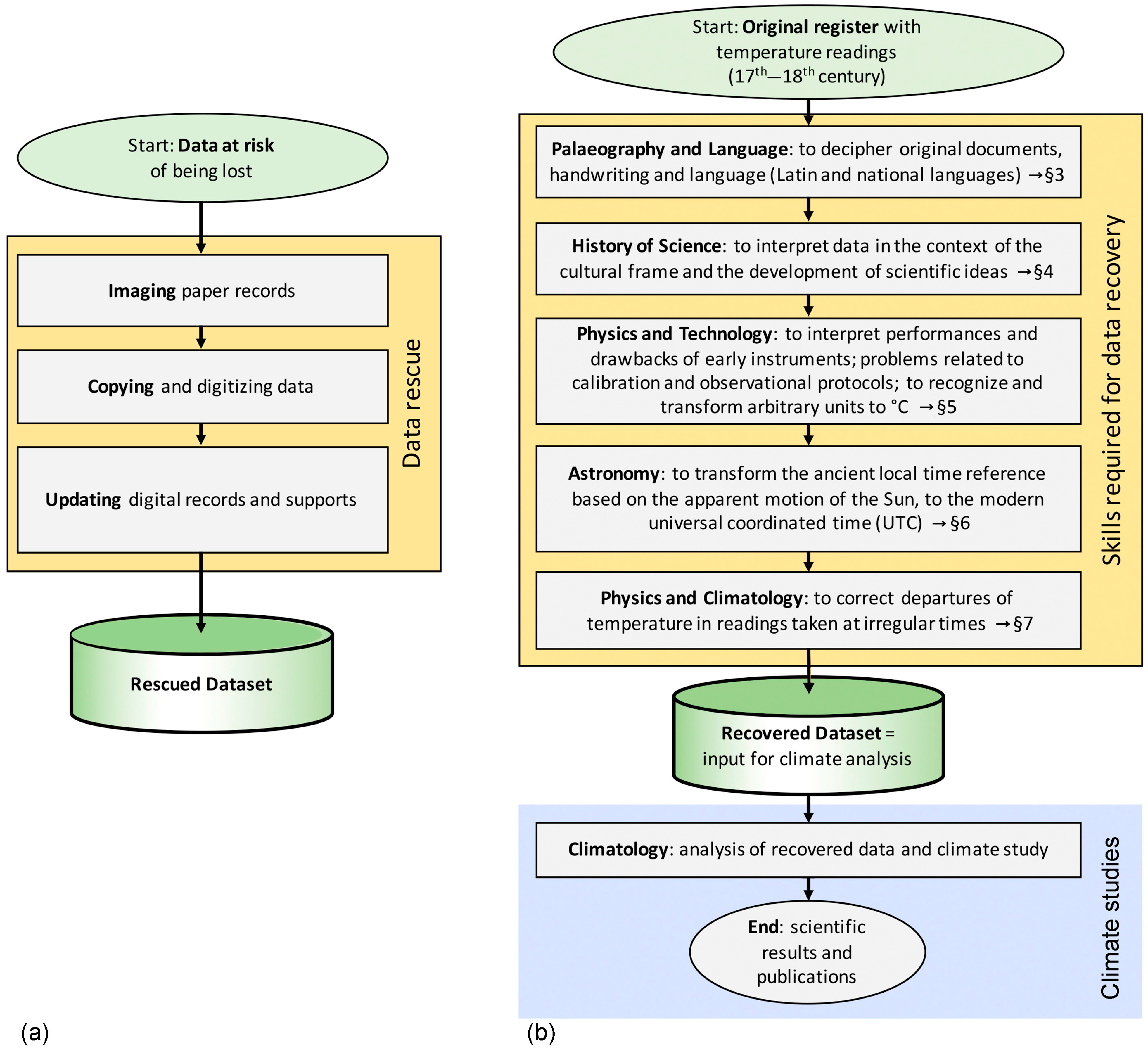
2. Aims and Structure of the Paper

2.1. Aims

For the complexity of the topics involved, the recovery of EIR requires experts, or specific skills, in a number of disciplines. Some climatologists work with a staff of colleagues with complementary skills (e.g., palaeography, ancient language, history, astronomy); others limit the field of research to what their skills can reach and cannot fully exploit EIR; only a few have a comprehensive background including the basic knowledge of the required disciplines. These difficulties explain why most EIR are still unknown and unexploited.

The purpose of this article is to illustrate the methodology used to recover the early temperature records (i.e., 17th, 18th, and the first half of the 19th century), taking advantage of previous studies performed with the earliest Italian thermometric series. Therefore, the article is a review-guide, intended to help young colleagues who want to tackle the difficult task of data recovery, by explaining the methodologies necessary to afford and solve the various difficulties, taking advantage of clear examples.

The focus is on the operations that should be performed to interpret, correct, and transform the original raw data into a high-quality dataset of temperature, usable for climate studies (i.e., the yellow box in Figure 1b). The aim is to assist in this task with a comprehensive review focused on the steps grounded on other disciplines with respect to climatology. Sections containing well-known topics will be short, while more detailed explanations will be reserved for the topics typical of other disciplines, likely less familiar to pure climate scientists.

This methodology follows the process that starts immediately after the discovery of an ancient register of weather observations with handwritten notes and numbers that should be transformed into a sound temperature dataset, ready to be used as an input for climate analysis. The study, use, and application of the recovered dataset (i.e., the cyan box in Figure 1b) are outside the scope of this paper.

2.2. Structure

The structure of the paper is divided into operative sections (Figure 1b). The starting point is when a register of EIR is found, and one wants to recover data and metadata.

Section 3. The first difficulty is to read and interpret the original log, data, and notes. The handwriting was made in ancient style, has been discoloured, stained, and damaged over time, is difficult to read, and needs a palaeographer. The language may constitute a problem, because most old documents are in Latin or in the local language, with ancient local, arbitrary or unknown units or there are additional metadata, e.g., letters exchanged with other scientists from other countries. An arbitrary unit is not based on known references and predetermined fixed points, but constitutes a casual scale related to a specific instrument. An unknown unit is a unit that was not explained or documented by the observer.

Section 4. The history of science is necessary to interpret the original text within the cultural frame of that time and the development of scientific ideas. It helps to interpret, or guess and then verify, the choices of the observer, in terms of instrument, exposure, time of reading and so on.

Section 5. Physics and technology are needed to interpret performances and drawbacks of early instruments, as well as the problems related to calibration and observational protocols, to recognize and transform arbitrary, or unknown units to °C.

Section 6. The time of readings was based on the local Solar Time as it appeared on sundials, based on the solar motion and the local meridian. Since the apparent motion of the Sun does not appear homogeneous to a terrestrial observer, this continuously shifted the time with reference to a modern clock. Furthermore, Italy and some other European Countries continued the Roman and Mediaeval use of the day that began at twilight, not at midnight. The transformation from the ancient time reference to the Coordinated Universal Time divided into Time Zones related to certain reference meridians (as we use today) requires a series of complex calculations. Moreover, it is not possible to make a simple table to transform the local apparent Solar time to modern time because the transformation changes with the calendar day, as well as the latitude and longitude of the site.

Section 7. In the early instrumental period, the observations constituted an additional, secondary task of the observers, and the reading times could change by one or more hours. The irregular sampling requires a further correction, not just for the time, but for the temperature change rate, i.e., to calculate the most likely temperature expected if the reading was taken at the scheduled time.

3. Registers, Data and Metadata: Handwriting and Language

Depending on the observer and the conservation, registers can be found ordered, or very messy, stained by water and ink; often, the ink of the back page has crossed the page and is superimposed on the poorly written and hardly legible words, numbers, symbols, and letters. Reading documents of the 17th or 18th centuries requires a specific skill in palaeography for deciphering and interpreting the handwriting, which generally includes abbreviations and symbols typical of the period and the cultural environment. The official language of educated people of the time, often university professors or priests, was Latin. Sometimes the local language was used in the registers, with raw annotations and obsolete terms.

Metadata help to identify instruments and observation protocols and are fundamental for data interpretation. Unfortunately, it is rare to find all the necessary metadata, and the obscure items should be recognized with particular tests, as discussed later. The original registers are fundamental for copying the data from the original source, paying attention to reading the data correctly, especially when they feature bad handwriting and obscure units.

A very popular use that can generate confusion is that the signs ‘−’ and ‘+’ for negative or positive values, or a note ‘below’ or ‘above’ (implying below or above 0°R) were not associated with every number, but were considered a benchmark written only the first time the reading dropped below zero, or rose above it (Figure 2). After this first minus (or ‘below’), it was considered obvious that all the readings were negative until the signal returned positive, and the turning point was marked with a plus (or ‘above’). Sometimes the benchmark was repeated for a few consecutive times, and then interrupted. This practice may be confusing, especially when the first minus or plus are hardy readable for water or ink stains, discoloured ink, or other drawbacks typical of early manuscripts. When data are simply rescued, the numbers are just copied. A period of intense cold with the temperature always below zero, e.g., a week, represented by only the first reading below zero and all the subsequent ones without sign, may be misinterpreted and considered positive. A period of intense cold can be mistakenly transformed into a mild period. The interpretation of the writing style is fundamental in correct data recovery.

Sometimes, the original registers have been lost, and it is necessary to rely on printed data, either daily, or monthly or yearly averages. This situation is not the best but constitutes the only possibility of knowing early climate data in certain regions.

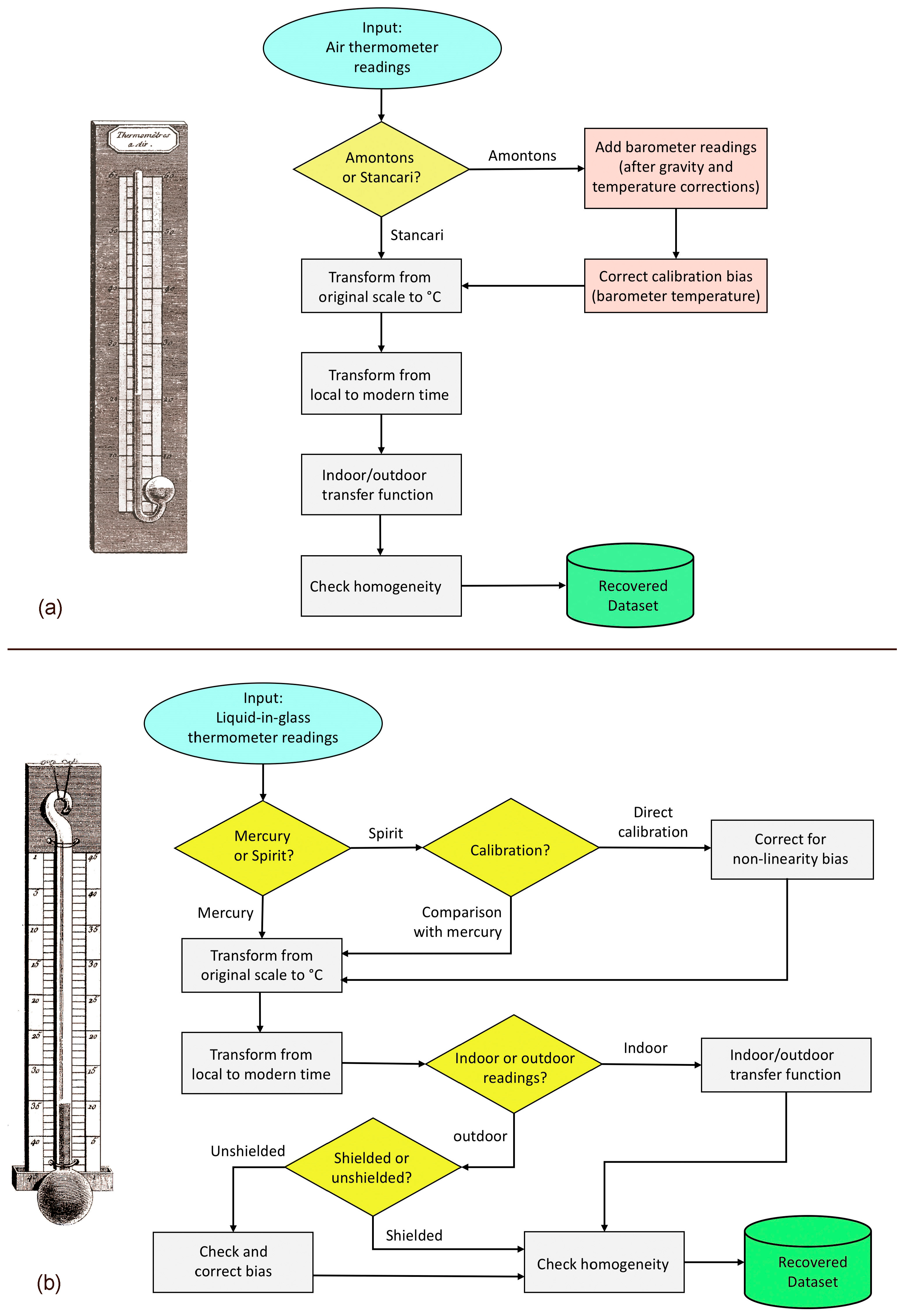
4. Short History and Technical Problems of Early Thermometers

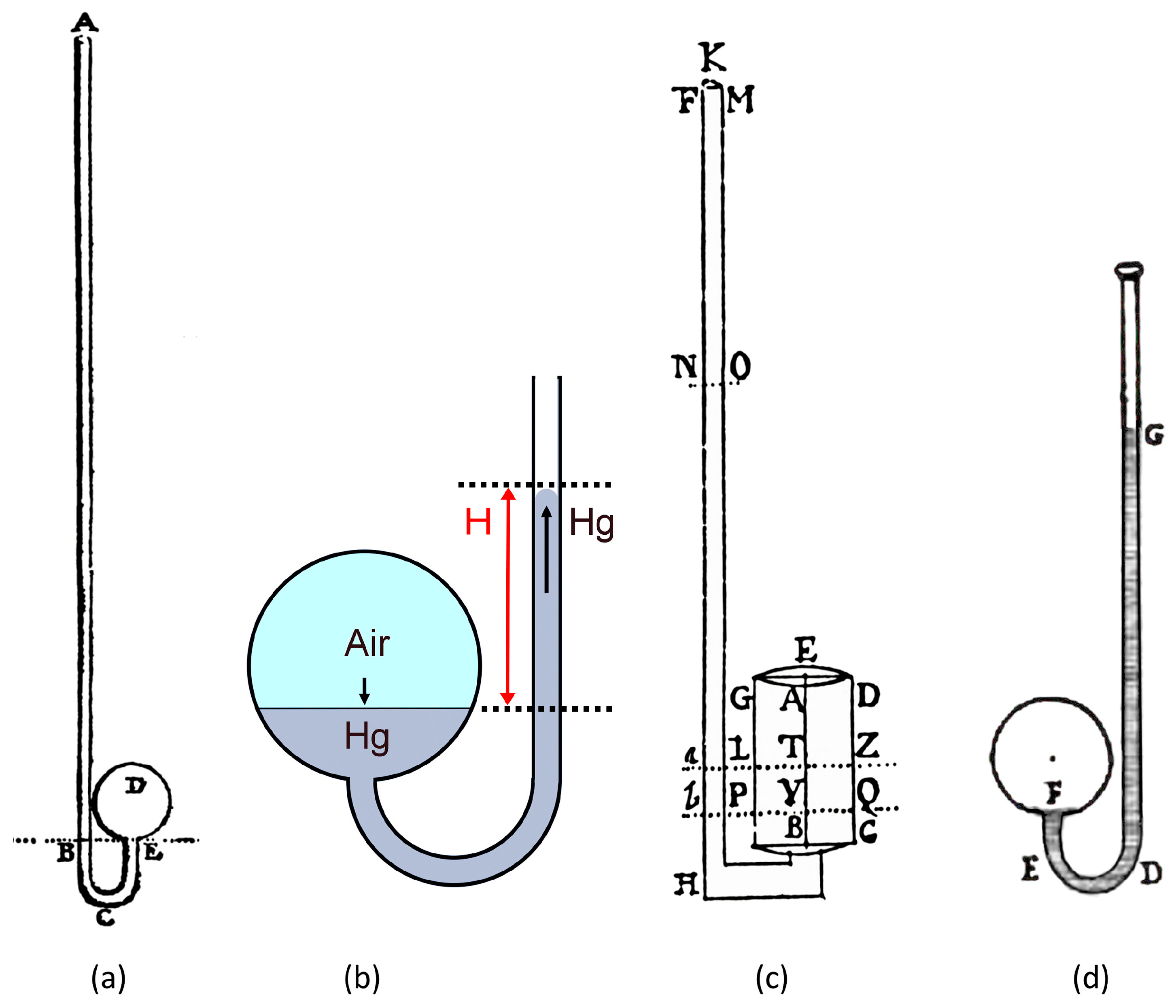
4.1. The Origins, and the Thermoscope

The history of thermometers has been the object of several studies [21,22,23,24,25,26,27,28,29,30,31,32,33,34]. The original idea on which the thermometer is grounded has been attributed to two ancient philosophers, i.e., Philo of Byzantium (2nd or 3rd century BC) [35], and Heron (also known as Hero) of Alexandria, Egypt, (c.10–70 AD) [36] who invented fountains and other amazing devices driven by water and air. However, when the thermoscope was invented, the books of Philo were unknown, probably because they were written in Greek and Arabic. Conversely, in the second half of the 16th century, the book of Heron, Spiritalia, was translated from Greek to Latin [37], then to Italian [38,39]. In addition, at the beginning of the 17th century, Della Porta [40] published a similar fountain. Heron became popular because his book contained detailed explanations of each device with the operating principle, and illustrated with a figure.

Galileo Galilei, Sanctorius Santorius and Cornelius Drebbel read these books and were stimulated to build devices where a pocket of air, when heated, displaces a column of water. Robert Fludd was unable to read the text but could interpret the drawings. These scholars invented their devices independently from each other, so the thermoscope was invented several times [34]. Galileo and Sanctorius gave the most scientific contributions. Galileo started around 1593, and considered the relationships between temperature, pressure, and volume. In 1641, the last year of the Galileo’s life, Robert Boyle went to Florence and returned home to study the laws of gases with a replica of a Florentine thermometer. Sanctorius [41,42] added a quantitative scale to the instrument to read the ‘heat’ (which was the old name for temperature) levels, or the ‘heat’ changes. In 1598, Drebbel applied the principle of the thermoscope to build an astronomical water clock powered by solar energy. Fludd [43,44,45] built solar fountains, applied the principle of the thermoscope to build a gigantic water calendar, and built some thermoscopes similar to Sanctorius.

In the thermoscope, the expansion of the air pocket was determined by both the temperature and the atmospheric pressure, which was unknown till 1643, when Evangelista Torricelli and Vincenzo Viviani discovered it. However, it soon became clear that the thermoscope had a problem, i.e., it was not stable for changes of atmospheric pressure and was abandoned.

4.2. Liquid-in-Glass Thermometers

In Florence, the Grand Duke Ferdinand II, Galileo, and the members of the Accademia del Cimento realized that not only air, but also liquids change density (and volume) with temperature, and started measuring the density of springs, rivers, spirit beverages, and many other liquids. This suggested the idea that a hermetically sealed phial of glass, containing inside a certain amount of alcohol and some air as well, would have caused the expansion of both, but being both enclosed in a fixed volume, the strength of the liquid would prevail over air and the length of the liquid column could be related to the ‘degree of heat’, i.e., the ‘temperature’, as it was named later.

The basic thermometer was the so-called Little Florentine Thermometer (LFT), invented around 1641 [23,24,25,46,47,48]. It was uniquely made of glass, except for the thermometric liquid, so that it could resist any weather. The scale was composed of 50 enamel bids, and a range that could respond to the cold waters of the Arno River in winter, and the hottest days in summer. The response time was about 5 min [49]. To interpret and make the readings of different thermometers comparable, the Grand Duke ordered the building of a large number of instruments, all with exactly the same size and quantity of alcohol, and the scale was fixed by comparison with a reference prototype. Thermometers with different responses were rejected. At this point, all the LFTs gave comparable readings, and the Grand Duke organized an international Meteorological Network, i.e., the Medici Network, which operated from 1654 to 1670, with thermometer readings every 3–4 h in Florence and Vallombrosa, and fewer readings in other stations [50,51].

The Florentine Academicians tested various thermometric liquids, including spirit (ethyl alcohol) and quicksilver (mercury). They preferred to use refined alcohol, i.e., the so-called acquarzente (wine spirit or burning water), that was obtained by distilling grapes twice, until the spirit reached some 80% ABV (alcohol-by-volume). The Academicians, and after them, Réaumur, as well as other scientists, preferred spirit to mercury because it expanded six times more, had a lower freezing point, was lighter and, in addition, cheaper. Robert Boyle preferred mercury; Daniel Gabriel Fahrenheit in 1709 built alcohol thermometers, but after 1714 he preferred mercury. Isaac Newton used linseed oil, but the oil was soon abandoned because it adhered to the capillary tube and made readings difficult. In Italy, two thermometric liquids were used: spirit (the most popular) and mercury. Spirit had two problems, i.e., the deviation from linearity of spirit depends on the ABV composition; once the thermometer had been built, the deviation of the thermometer depended on how calibration was made, i.e., with two fixed points, or by comparison with a mercury thermometer (Section 5). Mercury was a good choice because its response is linear and the calibration easy.

4.3. Air Thermometers

The thermoscope was abandoned because readings were biased by the atmospheric pressure. However, the idea of using air as thermometric fluid remained appealing for several reasons: (i) air is the most sensitive fluid to temperature, with a volumetric expansion coefficient of 3400 × 10⁻⁶ (1/°C), much greater than ethyl alcohol’s 1100 × 10⁻⁶ (1/°C) and mercury’s 180 × 10⁻⁶ (1/°C); (ii) all thermometers could have the same fluid with the same composition, expansion, and scale; (iii) air does not freeze; (iv) air is light; (v) air has no cost; (vi) in theory, only one calibration point would be sufficient, but in reality, two were needed. At the turn between the 17th and the 18th century, two scholars discovered how to solve the pressure drawback.

At the beginning of the 18th century, Guillaume Amontons [52] considered that the atmospheric pressure was counteracting the pressure of the air pocket enclosed in the spherical bulb. Therefore, his solution consisted of adding the height of the barometer column to the height of the thermometric column. Readings of the air thermometer, taken alone, had no meaning, but the sum of the thermometric and barometric readings gave the actual temperature. So, the temperature measurement needed two instruments. This was not a problem for a fixed station, but it could be for field measurements that required the moving of two delicate instruments. The thermometer was J shaped, with a spherical bulb containing the (compressed) air pocket sealed to the lower end of the J shaped tube, while the upper end of the tube was open (Figure 3a). A thermometer with open tube was obliged to use mercury, because ethyl alcohol is volatile and would have evaporated in a short time. In addition, the weight of the mercury increased the reactive spring of air.

The Amontons thermometer had other problems. (i) Depending on the temperature and the pressure in the air pocket, some molecules of water vapour could condense, lowering the reading. (ii) The air pocket was in a spherical bulb, compressed by the column of mercury (i.e., the distance between the upper meniscus on the tube and the free surface of mercury in the bulb). In the air pocket, any change in temperature or pressure displaced a certain volume of mercury that passed from the sphere to the column (Figure 3b). However, the free surface of the mercury moved up and down in the spherical bulb. This surface constituted a circular cross section with variable radius. Under the same volume change of the gas, a different section of the mercury in the bulb resulted in a different height H of the mercury displaced in the column of the capillary tube, measured from the free surface of mercury in the spherical bulb. Therefore, although this thermometer used linear fluids (i.e., air and mercury), its response was not linear. To avoid this drawback, Giovanni Poleni used a cylindrical bulb: the constant cross section provided a linear response [53] (Figure 3c). (iii) The calibration was another crucial item, as discussed later (Section 5.6). In Italy, the Amontons thermometer was used by Giovanni Poleni in Padua (from 1725 to 1761) and Tommaso Temanza in Venice (from 1751 to 1755).

In the same period, in Bologna, Vittorio Francesco Stancari [54] considered another approach [55]. He built exactly the same J shaped glassware with the spherical air pocket on the lower end but sealed the upper top of the tube without leaving air inside (Figure 3d). Therefore, the upper part of the tube was empty, except for the vapour of mercury, and the height H of the column with reference to the free surface of mercury in the bulb was uniquely determined by the temperature. This thermometer had the above-mentioned problems of the change of phase of some moisture, and the non-linearity caused by the spherical bulb. However, it was a self-sufficient instrument and avoided the drawback related to the barometer. This thermometer was used by Jacopo Beccari and co-workers in Bologna (from 1715 to 1737).

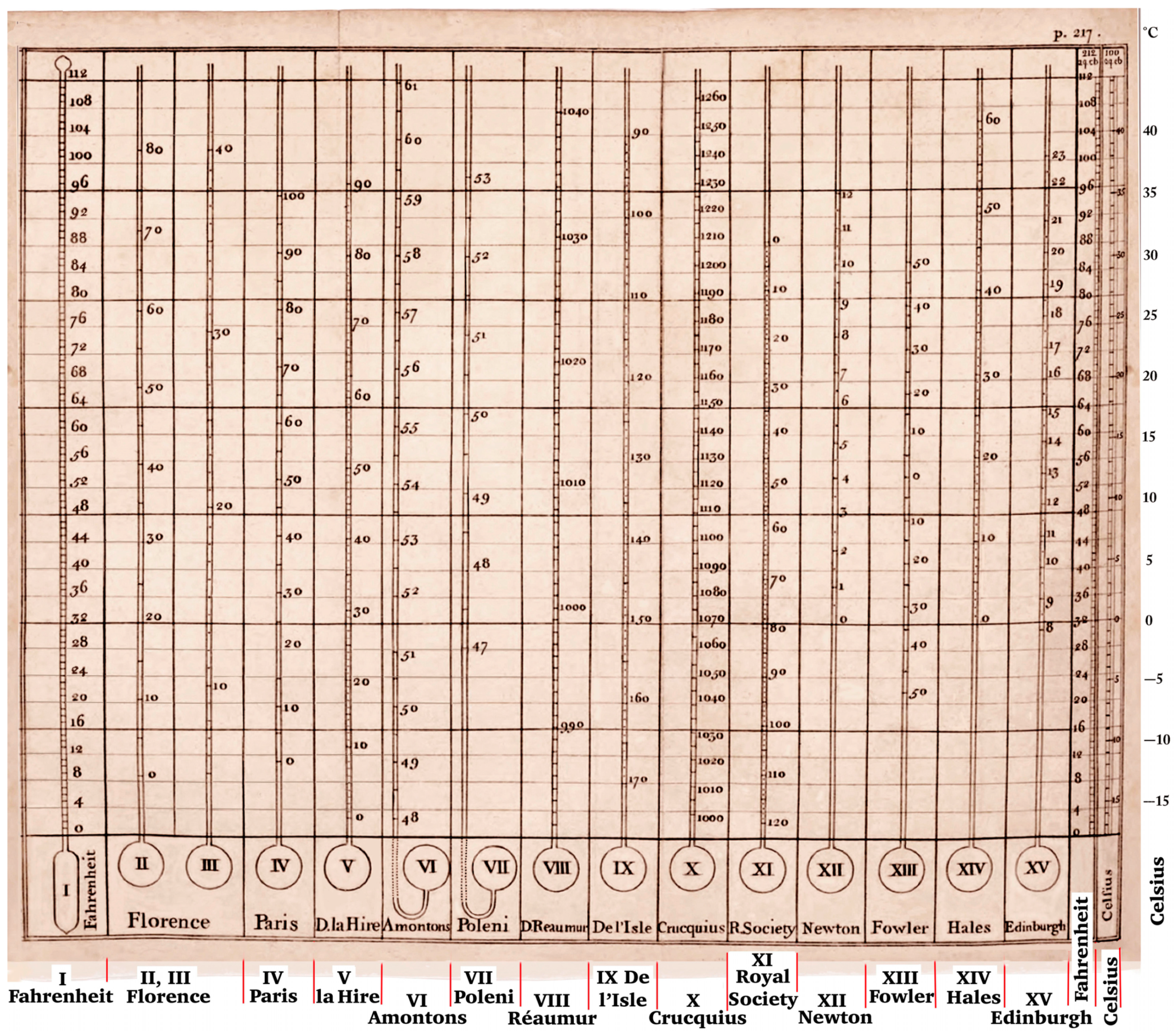
5. Scales and Calibration

5.1. The Thermometric Scale

The scale was used to read the height of the thermometric liquid in the graduated column, and this could be done starting from the base (i.e., direct scale with increasing values as the temperature increased) or from the top (i.e., reverse scale with decreasing values as the temperature increased). The Little Florentine thermometer only had bids, but no numbers, and could be read in either direction. All early thermometers had a scale, but not the same one. The scale of the air thermometers had to be adjusted at every reading to follow the level of mercury in the spherical bulb.

5.2. When the Scale Is Unknown

Some observers published their data without specifying the scale that was in arbitrary units AU. Deciphering these arbitrary units, each one different from the other, poses a very difficult problem. The scales used by Beccari in Bologna have been recognized [56]; the scale used by Temanza in Venice will be considered in the near future, taking advantage of the contemporary series in Padua.

A very useful piece of information is when the log contains notes about the weather. If the observer registered when it was snowing, we can take note of the AU temperatures of the snowing days, and consider that snowflakes may fall either at temperatures below 0 °C, but also some degrees above 0 °C if the air is dry enough, because vaporization lowers the temperature of falling snowflakes [57,58,59]. This fact may be used to calibrate thermometers [34]. The method consists of dividing the temperature in narrow intervals, each of them constituting a bin, and putting in each bin the number of times snowflakes were observed in that temperature interval (Figure 4). After comparison with known temperature values, it has been found that 0 °C may be recognized as the upper inflexion of the bell-shaped histogram representing the number of snow days versus temperature. This method has been used in a number of case studies [49,56,60].

Unfortunately, there is not a natural phenomenon to take advantage to recognize the upper part of the scale. If there is another contemporary record in the same locality or nearby, and we know the relationships between the two sites, it is possible to compare the average values of the same summer months in the two sites. This may give a crude but realistic indication.

5.3. Fixed Points for Calibration

To make readings comparable, some fixed points have been suggested since the early period, e.g., Christian Huygens [61] and then Carlo Renaldini [62] suggested the melting point of ice and the boiling point of water; Joachim Dalencé [63] the freezing of water and the melting of butter or the melting of ice and deep cellars; Isaac Newton [64] the melting of snow and the blood temperature of a healthy adult male; Olaf Christiansen Roemer [23] a mixture of sea salt and crushed ice and, in addition, the blood temperature; Philippe de la Hire [65] the freezing of water and the cellars of the Paris Observatory; Daniel Gabriel Fahrenheit [66] adopted a three-point calibration, i.e., the mixture of ice and ammonium chloride, the melting of ice, and the body temperature; Jacques Barthélémi Micheli du Crest [67] the underground caves of the Observatory of Paris and boiling water; Anders Celsius [68] the centigrade scale, but inverted. In the 18th century, there were plenty of scales. Martine in 1740 [69] (Figure 5), followed by Cotte in 1774 [70], published a table that compared 16 of the most popular scales in the first half of the century, and Landsberg [27] a table including 36 scales. It is surprising to find in Martine [69], in the last column, the Celsius scale, not the original reversed form (i.e., 100 °C at the freezing and 0 °C at the boiling point) but as we use it today. In addition, it was published in 1740, i.e., two years before the official publication by Celsius [68]. This suggests that Celsius published it some years after it was proposed and used [71]. In Italy, the Celsius scale became popular at the end of the 19th century, substituting the largely dominant Réaumur scale.

Although calibration points constituted a significant step forward, they were not always applied correctly, or they were not suitable for the thermometer. For example, many winter days were below the melting temperature of ice, especially on the mountains or the polar regions. This required an additional lower point, determined with a solution of brine made from a mixture of water, ice, and ammonium chloride. The ammonium chloride was substituted with sodium chloride (marine salt), which was cheaper but provided a slightly different value. Toaldo [72] noted that the uncertainty was of 5 °R, i.e., around 6 °C. Similarly, the point of boiling water was not realistic for normal weather, indoor temperature, or feverish sufferers, and required too long a graduated column of which only a small fraction was used, e.g., 1/3. The upper limit based on the human body temperature (i.e., around 33–38 °C) was not well defined, but more convenient for everyday use, because it was a good reference for the hottest days in northern Europe. Although these pragmatic calibration points were more viable, they had an uncertain definition. Nevertheless, they were more convenient to represent the upper and lower borders of the range of interest.

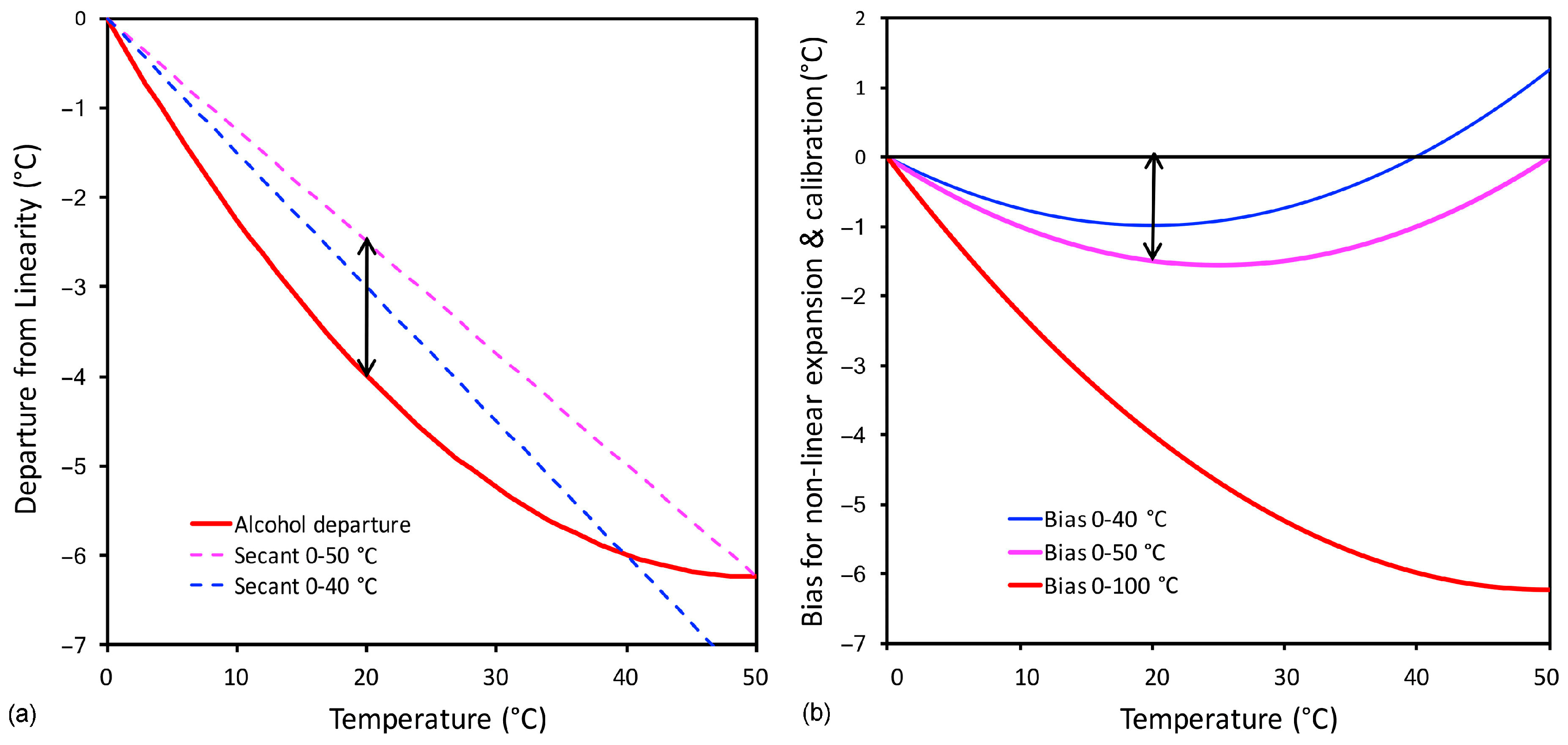
5.4. Deviations from Linearity, the ‘True’ and the ‘False’ Réaumur Scale

A serious difficulty was that, after calibration, wine-spirit thermometers had non-comparable readings [67,69,73,74,75,76,77,78,79,80]. The fact that these thermometers had the same fixed points, but different intermediate values, meant that the deviation from linearity was not always the same, because it changed with the purity of the alcohol. This posed a very serious challenge to the scientists of the 18th century. Réaumur [81,82] conceived a single calibration point, i.e., freezing water, but added some additional reference points, i.e., the cold mixture of ice and salts, the body temperature, the temperature of the cellars of the Meteorological Observatory in Paris, and boiling spirit. The initial idea of Réaumur was to build a universal thermometer, with a calibration made adding known small volumes of spirit using phials of known volume, operating at room temperature. However, in his experimental apparatus, Réaumur made some misinterpretation about the boiling point of spirit and water and which of them should be attributed to 80 °R. The result was the so-called ‘True Réaumur’ thermometer, as De Luc [75] named it, that had 80 °R (equal to 80 °C) as the boiling point of spirit and is close to the Celsius scale [71]. Thermometers with the ‘True Réaumur’ scale were built from 1730 till 1740, when Martine [69] made some serious criticisms to Réaumur.

Martine [69] wrote: the boiling point is ‘very erroneously graduated’; ‘Réaumur was in the wrong’ when he evaluated the boiling point with a confusion between spirit and water; the calibration made with phials at the same temperature disregarded the fact that glass and wine-spirit expand differently. This obliged Réaumur and Jean Antoine Nollet, his pupil and instrument maker, to change their minds [83,84]. From Nollet we know that the revised Réaumur thermometers, built after 1740, were calibrated fixing 80 °R at the boiling point of water, i.e., 100 °C. De Luc [75] named this revised generation of thermometers (i.e., 80 °R = 100 °C) ‘False Réaumur’ to distinguish them from the previous generation of ‘True Réaumur’ (i.e., 80 °R = 80 °C). The ‘False Réaumur’ is the scale of the popular Réaumur thermometers that have been used worldwide, especially in the 19th century [71,85,86], and was adopted by the Network of the Societas Meteorologica Palatina, Mannheim [87].

About the revised Réaumur scale, Nollet [84] was clear in text and illustration (Figure 6). The figure shows a pot of boiling water and a tub of crushed ice in which the thermometers were dipped. There was a large thermometer with long capillary tube, called primary, and several small thermometers that were compared to the primary one, and the level of the spirit in the tube was marked with a silk thread, well visible in the figure. On the table, a serving stand holds some glass phials for the volumetric calibration.

In general, the level of the meniscus at the calibration points was marked by knotting a silk thread on the capillary, and then dividing the length L of the capillary between the two fixed points in a selected number of equal intervals (e.g., 80 for the Réaumur scale, so that 1 °R = L/80) and extrapolating these divisions on the side of the intense cold.

The method was fine for liquids with linear expansion, e.g., mercury above 0 °C, linseed oil [88], but not for alcohol that deviates from linearity. In addition, ethyl alcohol has a deviation that increases with the proportion of water mixed to it. On hot summer days, at 40 °C, the readings were underestimated by 4–5 °C [89]. Alcohol thermometers with spirits not at the same purity level gave different readings, and even more different from mercury thermometers. The data comparability was a hard problem in the 18th century. The difference ∆(T_Hg,a) between the reading of a mercury (T_Hg) and of a well-purified (e.g., 95% ABV) alcohol thermometer (T_a) (Figure 7a) is [89]:

$$∆\left(T_{Hg,a}\right)=T_{Hg}-T_a=-0.0025T_a^2+0.2497T_a$$

(1)

The reading T_a may be converted as it was taken with a mercury thermometer (T_Hg) using the inverse formula [89]:

$$T_{Hg}=-0.0025T_a^2+1.2497T_a$$

(2)

5.5. Calibration by Comparison with a Mercury Thermometer

Things were different if the spirit thermometer was not calibrated at the fixed points 0 °C and 100 °C, but by comparison with a primary (i.e., mercury) thermometer at two points, e.g., 0 °C and 40 °C, or 0 °C and 50 °C (Figure 7a). At the calibration points, the readings are correct. For other temperatures, the bias is limited to the departure of the quadratic curve of non-linear expansion of alcohol from the secant that joins the two calibration points, e.g., 0 °C and 50 °C. The secants represent a linear interpolation between the two calibration points, which is the behaviour of a mercury thermometer. Therefore, the departure of the quadratic curve from the secant represents the bias of a spirit thermometer with calibration made by comparison, with the upper point lower than 100 °C (Figure 7b). When calibration is made by comparison with a mercury thermometer, the maximum bias is strongly reduced, and is of the order of magnitude of 1° to 1.5 °C. For the temperatures selected for the Little Florentine Thermometer, the bias was within ±0.5 °C [89].

Excellent results were obtained if the calibration of the spirit thermometer was made at a number of selected temperature levels by comparison with a mercury thermometer as suggested by Cavendish [90,91]. The two thermometers were dipped in the same bath, e.g., a pot of hot water, where the temperature was allowed to decrease very slowly. When the column of the mercury thermometer reached some selected levels, e.g., 50°, 40°, 30 °C and so on, the instrument builder knotted a silk thread on the capillary of the spirit thermometer and reported the same values on the scale. Therefore, these reference values were the same as the thermometer used for calibration, and the intervals between two consecutive benchmarks were divided linearly. However, if the interval was relatively small, e.g., 10 °C, the departure was negligible.

5.6. Calibration of the Amontons Thermometer

For the Amontons thermometer, the calibration should be made considering both the Amontons thermometer and the barometer operating simultaneously. In the 18th century, the barometric corrections for gravity and temperature were not applied. Likely, the calibration was preferably made in winter to have ice available, and the freezing point was established with both instruments kept around 0 °C. In contrast, the upper limit was established with just the bulb of the thermometer held in the hot steam of a boiling pot of water, while the barometer was left cold [91]. The combination of hot thermometer and cold barometer was unrealistic because in the real world both instruments operate in the same room and at the same temperature. This required a specific correction, by calculating the true pressure and the expected bias for this difference.

6. Transformation from the Ancient to the Modern Time Frame

6.1. The Canonical Hours of the Italian Time

In the antiquity, most of Europe followed the tradition of the Roman Empire, of starting the new day immediately after the previous died, i.e., at sunset. For most countries, this practice continued over the Middle Ages, and the hours were announced with bells from the tower clocks, i.e., the so-called ‘canonical hours’ or ‘Italian Time’ [92,93]. The political events partially changed this situation, but Italy, Poland, Bohemia, Silesia, Portugal, and some others followed the tradition of the canonical hours till the end of the 18th century.

In Padua, the change of the day starting from sunset to midnight occurred in 1789 and was repeated in 1790 with the cooperation of Toaldo [94,95,96] but was soon abandoned because it created havoc for the population. The real change occurred when it was imposed by Napoleon in 1797 [97]. The Decree was short, and established that it was mandatory for all clocks, either public or private, in the city or the countryside, to change from the Italian to the French time. An instruction was enclosed, to explain the new frame and a table with the correspondence, hour by hour, between the two timeframes [98]. This instruction was presented in anonymous form, but the author was Toaldo. The reference was the solar culmination on the local meridian. Every city had an own decree signed by both the provisional municipality and the French military commander. These transitions occurred in the years 1796 and 1797.

Theoretically, for every site, the new day started at twilight, when everyone fell into darkness. This was the most popular tradition. However, the time of darkness was not well defined because on clear days, twilight gained some 30–40 min of pale light, depending on the season, but in case of rain, cloud cover, or fog, darkness occurred earlier, e.g., an hour or even more. In addition, in the 18th century, wall sundials responded to the actual position of the Sun and mechanical clocks were adjusted every day at noon with the upper culmination of the Sun (i.e., the Sun passing through the local meridian); the sundials and clocks of cultured people responded to the actual Solar position, which could be related to the sunset (governed by precise astronomical laws), not dusk or twilight (governed by astronomy and uncertain weather factors).

The definition of when the day began was unclear. Some people preferred twilight because darkness was evident to everyone. Astronomers preferred the sunset, because it was objectively defined, but the people did not agree, because in the cities there was no a free horizon, and it was difficult to establish the precise moment at which Sun crossed it. However, given the imprecision of 18th century clocks, this did not make much difference. Toaldo [94,95,96,98] was clear on that issue, and published instructions and detailed tables with numerical values valid for the local meridian, to pass from the canonical hours of the Italian Time (day starting from the local sunset) to the French Time (day starting from the local midnight). Most EIR in Italy are based on this reference, and the ancient time must be transformed in modern time units. Astronomers were used to referring the position of the stars to the lower Solar culmination (i.e., local midnight when the Sun crosses the meridian from the opposite side of the Earth) and a minority of records follow this style.

EIR recovery requires a series of adjustments for time, which changed day by day, i.e., for the running day j of the calendar year, it is necessary to apply a number of astronomical corrections to transform the temporal frame based on the actual Sun motions, represented in spherical coordinates, to the Universal Coordinated Time (UTC) of the Italian Time Zone (UTC + 1) referred to the Greenwich Meridian. This requires calculating the solar declination over the year and combine it with the local latitude; the consequent change of the daylight time, characterized by the effective instant of sunset and the time elapsed to reach the local midnight; the combined effects of the eccentricity and obliquity that make the Sun’s motions appear slower or faster (i.e., the so-called equation-of-time to adjust these departures), and the correction for the difference of longitude between the local site and the time zone reference, as described in the following sections.

6.2. Solar Declination

The solar declination ${\delta }_{\odot ,j}$ of the running day j of the year is an astronomical variable necessary for calculating the exact time of sunset. To make calculations, an adjustment should be made because the civil year starts on the 1st of January, while the solar cycle starts with the winter solstice, on the 21st of December. This requires adding D = 10 days to j. When the precision of seconds is not relevant, the simplified equation is used:

$${\delta }_{\odot ,j}=-23.45cos\frac{2\pi \left(j+D\right)}{365}$$

(3)

The range of ${\delta }_{\odot }$ is ±23.44°.

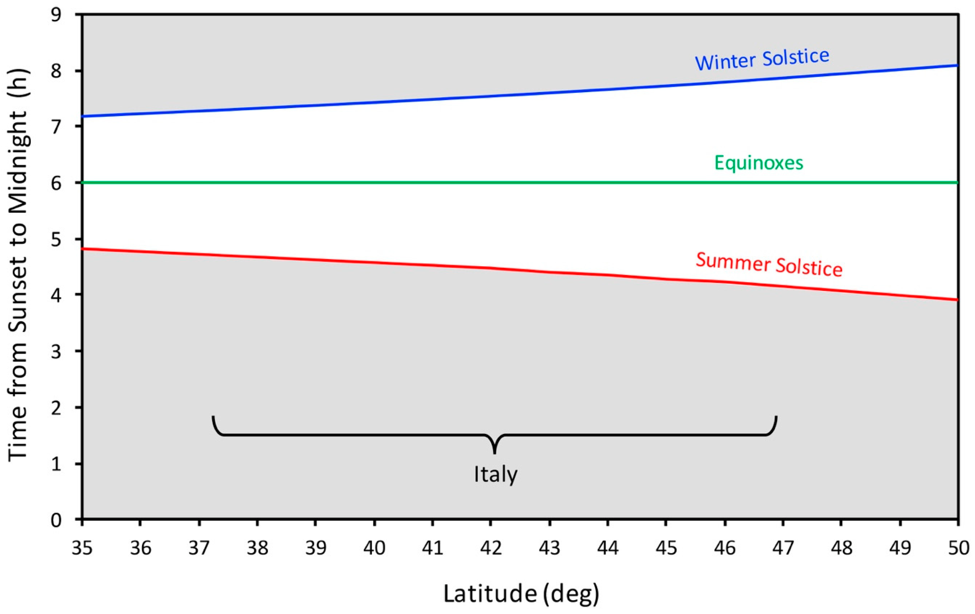
6.3. Time Elapsed from Sunset to Local Midnight

As the day started from sunset, it is necessary to subtract the time elapsed from sunset on the day j to the lower culmination of that day (i.e., the apparent local midnight). Then, the given hours are counted starting from the actual midnight, also variable with the calendar day j. Sunset may be found tabulated in astronomical or nautical almanacs with solar ephemerides, or may be calculated under the condition that the height H_⨀ of the Sun above the local horizon equals zero:

$$cos\tau =-tan{\delta }_{\odot }tan\varphi$$

(4)

where $\varphi$ is the latitude, and τ the astronomical hour angle 360°. The latter is transformed in 24 h clock time t with the equation:

$$t=\frac{12}{180}\tau$$

(5)

To make astronomical calculation easier, the t hours are considered after the upper culmination, i.e., midday assumed as t = 0; therefore, t < 0 in the morning, and t > 0 in the afternoon. After, t is transformed in accordance with the popular style 0 to 24 h, starting from midnight.

Equation (4) is represented in Figure 8. Both show, either mathematically or graphically, that the time from sunset to the lower culmination changes with the declination and latitude. It can be noted that cosτ vanishes for τ = π/2 (i.e., t = 6 h) when ${\delta }_{\odot }=0$, i.e., at the equinoxes. Extreme values are reached at the solstices. Except for equinoxes, the daytime duration (i.e., from sunrise to sunset) increases with the latitude. At the solstices, sunrises and sunsets each change by 3.522 min per degree of latitude, and the daylight duration by 7.044 min per degree of latitude. As Italy lies in the latitude belt from around 37° to 47°, the sunset in the northern borders occurs some 35 min later than in the southern ones, and the change in the daytime duration is twice this value, i.e., 1 h 10 min. Examples of values for 30 selected cities over Italy are reported in

Table 1. Example of 30 selected Italian cities, geographical coordinates, and time-related features.

City	Latitude North (°)	Longitude East (°)	Daytime Duration Winter Solstice (h)	Daytime Duration Summer Solstice (h)	Sunset to Local Midnight. Winter Solstice		Sunset to Local Midnight. Summer Solstice		Correction for Longitude (min)
					(h)	(min)	(h)	(min)
Aosta	45.7333	7.3167	8.48	15.52	7	45.7	4	14.3	−29.3
Alessandria	44.9167	8.6167	8.58	15.42	7	42.5	4	17.5	−34.5
Ancona	44.6167	13.5167	8.75	15.25	7	37.6	4	22.4	−54.1
Bari	41.1167	16.8833	9.03	14.97	7	29.0	4	31.0	−67.5
Bologna	44.5000	11.3500	8.64	15.36	7	40.9	4	19.1	−45.4
Bolzano	46.5000	11.3333	8.37	15.63	7	48.8	4	11.2	−45.3
Catania	37.5000	15.0833	9.41	14.59	7	17.8	4	42.2	−60.3
Ferrara	44.8333	11.6333	8.59	15.41	7	42.2	4	17.8	−46.5
Firenze	43.7667	11.2500	8.73	15.27	7	38.2	4	21.8	−45.0
Foggia	41.4667	15.5500	8.99	15.01	7	30.2	4	29.8	−62.2
Genova	44.4167	8.9167	8.65	15.35	7	40.6	4	19.4	−35.7
Lecce	40.3500	18.1833	9.12	14.88	7	26.5	4	33.5	−72.7
Lucca	43.8500	10.5167	8.72	15.28	7	38.5	4	21.5	−42.1
Messina	38.1833	15.5667	9.34	14.66	7	19.8	4	40.2	−62.3
Milano	45.4667	9.1833	8.51	15.49	7	44.6	4	15.4	−36.7
Modena	44.6500	10.9167	8.62	15.38	7	41.5	4	18.5	−43.7
Napoli	40.3500	15.2500	9.12	14.88	7	26.5	4	33.5	−57.0
Padova	45.4000	11.8833	8.52	15.48	7	44.4	4	15.6	−47.5
Palermo	38.1167	13.3500	9.35	14.65	7	19.6	4	40.4	−53.4
Pisa	43.7167	10.4000	8.73	15.27	7	38.0	4	22.0	−41.6
Potenza	40.6333	15.8167	9.09	14.91	7	27.4	4	32.6	−63.3
Ravenna	44.4167	12.2000	8.65	15.35	7	40.6	4	19.4	−48.8
Roma	41.9000	12.4833	8.95	15.05	7	31.6	4	28.4	−49.9
Siracusa	37.0667	15.2833	9.45	14.55	7	16.5	4	43.5	−61.1
Taranto	40.4667	17.2333	9.10	14.90	7	26.9	4	33.1	−68.9
Torino	45.0667	7.7000	8.56	15.44	7	43.1	4	16.9	−30.8
Trento	46.0667	11.1333	8.43	15.57	7	47.0	4	13.0	−44.5
Udine	46.0667	13.2333	8.43	15.57	7	47.0	4	13.0	−52.9
Venice	45.4333	12.3500	8.52	15.48	7	44.5	4	15.5	−49.4
Verona	45.4500	11.0000	8.51	15.49	7	44.6	4	15.4	−44.0

.

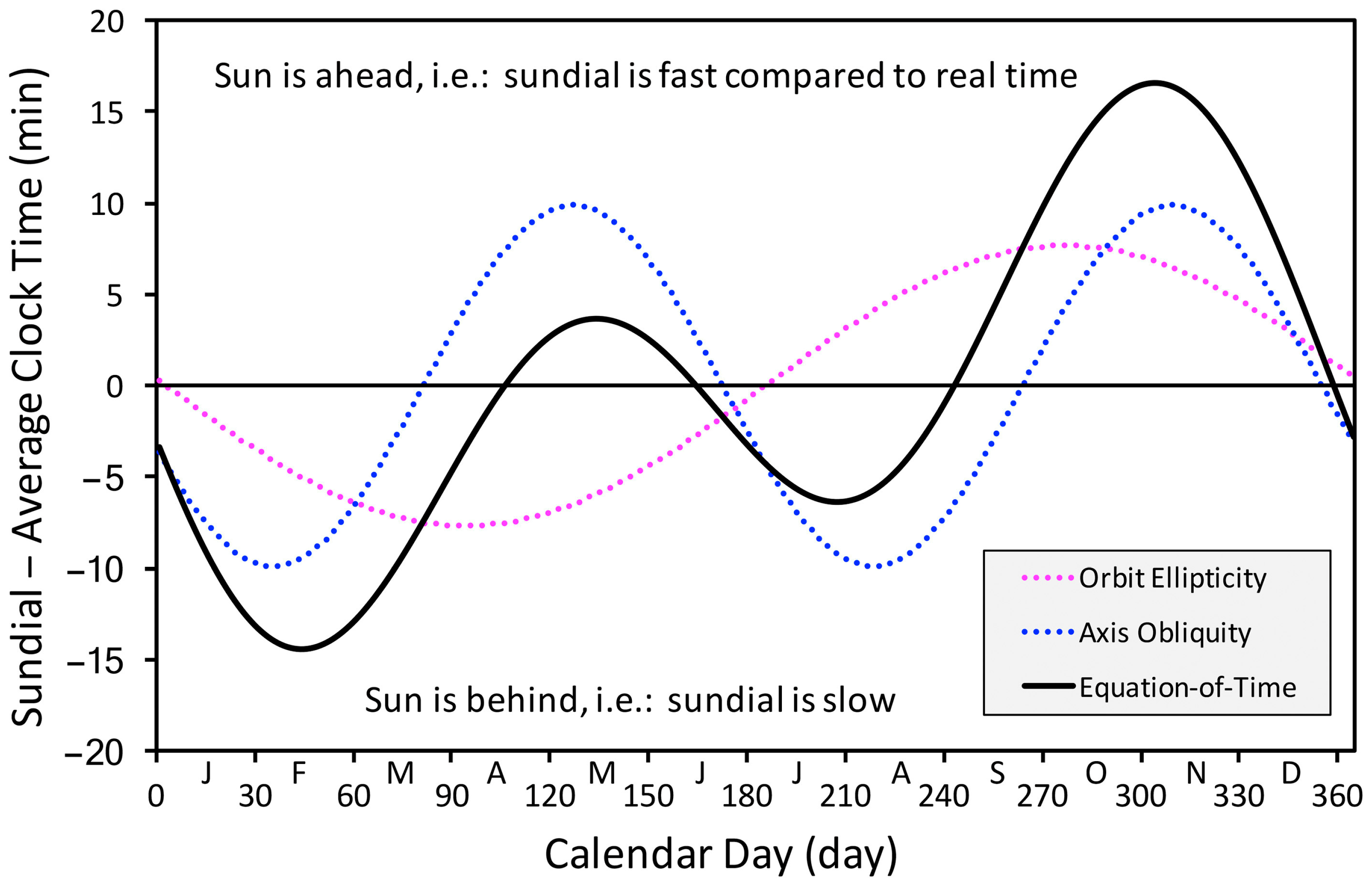
6.4. Equation-of-Time

The apparent motion of the Sun is uneven due to the combined effects of the yearly cycles of the eccentricity of the Earth’s orbit around the Sun, and the obliquity of the rotation axis of the Earth. The so-called equation-of-time (EoT) [99] represents the departure between the apparent solar motion of the running day j of the calendar year and the average solar motion over the year (Figure 9).

$$EoT=-7.66sin\frac{2\pi \left(j-P\right)}{365.25}-9.87sin\frac{4\pi \left(j+D\right)}{365.25}$$

(6)

where 365.25 days is the duration of the Julian astronomical year, and P the perihelion calendar day, i.e., 2 ≤ P ≤ 5 days (from January 2 to 5 depending on the leap or post-leap years). The departure ranges from −14 min 6 s (11th of February) to + 16 min 30 s (3rd of November). Leap years, as well as leap + 1 year, leap + 2 years, and leap + 3 years, change of the perihelion date, change of the winter solstice, Moon perturbation, and atmospheric refraction, will affect the mentioned dates a little (±2 days). The consequence on EoT values is within ±20 s, which is irrelevant for meteorological data. The secular change accounts for some 20 s per century, which is also irrelevant to our aims.

6.5. Correction for Longitude

For the rotation of the Earth, and the geographical location of the site, the local meridian is crossed earlier (longitude East) or later (longitude West) with reference to other selected meridians (i.e., local times are not simultaneous) and in particular to the reference meridian of the time zone. The departure $∆t_{\lambda }$ corresponds to the angular difference between the longitude $\lambda$ of the site and the meridian selected for the time zone (e.g., UTC + 1 makes reference to the meridian 15 degrees East of Greenwich), and the difference accounts for 4 min of time for every 1 degree of arc of longitude:

$$∆t_{\lambda }=4\lambda$$

(7)

Italy lies between the longitudes 6.6° and 18.5° East, which means $∆t_{\lambda }$ = −26.4 and −74 min, respectively, i.e., around 48 min difference between the most eastern and most western borders. The longitude corrections for 30 selected cities of Italy are reported in Table 1, last column.

6.6. From the Local Time to the Time Zone

In 1866, after Italy was unified and became a single state, all the cities adopted the mean local standard time of the Capital, i.e., Rome, with $\lambda$ = 12.452333° longitude East. On 1 November 1893, Italy adopted Central European Time (CET), i.e., Time Zone 1, or, in Coordinated Universal Time, UTC + 1. Therefore, the reference was changed to Mount Etna $\lambda$ = 15.00° longitude East that coincided with the First Meridian, 15° longitude East of Greenwich. The change of reference corresponded to −10 min; therefore, Italian readings made from 1866 to 1893 should be shifted by 10 min.

6.7. Transformation from the Italian Time to Modern UTC Time

The transformation from the ancient time t_CH in canonical hours to the present-day time t_PD is obtained by combining the previous departures:

$$t_{PD}=t_{CH}-∆t_{S-M}+EoT-∆t_{\lambda }$$

(8)

The exact transformation of time is crucial when one calculates the anomaly or investigates trends, because an incorrect transformation may cause consistent differences in the observing time and, consequently, in the related temperature [100,101]. More details about the methodology, as well as examples of specific case studies concerning selected Italian cities, Paris, and Switzerland, can be found in the literature [34,49,50,55,56,92,102,103,104,105,106].

The difference between the apparent solar time (as observed with a sundial) and the official modern UTC time (i.e., Coordinated Universal Time) of 92 selected sites over Europe, lying in the time zones UTC + 0, UTC + 1, and UTC + 2, has been calculated by Camuffo et al. [93]. Over Europe, the departures between a sundial and the related time zones range from −100 to +40 min. An example of the difference between the local time of sundials in Italy and UTC + 1 (calculated disregarding the change of 1 h in summer to save energy) is here reported for 22 Italian cities (Figure 10). The belt width is 35 min, from the eastern Lecce on the top, to the two western cities on the lower border, i.e., Aosta and Torino (overlapped). The most extreme departures are around −45 min, reached in February, and +30 min in November.

7. Reading Times

7.1. Impact on Indoor or Outdoor Measurements

The long series are affected by changes in reading times, either random or systematic. When the measurements of EIR were taken inside, in unheated rooms, people considered that the room temperature was mainly constant over the day, so that readings were taken at the observer’s convenience around a selected time, e.g., when the observer woke up in the morning, or when he returned home for lunch, or in the evening after dinner. Some observers carefully followed the established protocol; others made observations at random times.

With indoor observations, the daily cycle was smoothed by the building envelope, so that a small change of reading time caused a negligible departure. However, indoor readings are difficult to relate to the outdoor temperature. Sometimes, there is the lucky opportunity to find an outdoor series with a common sub-period. If the data over the common sub-period are represented in a scatter plot, i.e., the indoor versus the outdoor readings, by interpolating the dots with a polynomial fit, it is possible to obtain the transfer function and transform the whole period of indoor readings as if they were taken outside. For instance, Poleni observed indoors, once a day. The parallel series by Morgagni, who measured both indoors and outdoors, was of little help, because his external thermometer was biased by the thermal inertia of the thick walls. It has been necessary to find the indoor/outdoor transfer function of the Beccari house [56], which was a similar building, to transform the Poleni dataset as if it was taken outdoors [107,108].

With outdoor observations, the regularity of the reading time is highly relevant, and a key problem is how many observations were made per day. Some different cases are considered in the next section.

7.2. Readings Made at Irregular Times

Especially in EIR, it is frequent to find that an observer planned some reading times, e.g., when he woke up and after lunch, but readings were then made earlier or later. Depending on the hour of the day, and the season, the departure from the reading time may cause a consistent bias in temperature. A methodology has been adopted to correct several case studies [49,56,60,92,93,104,108]. The method consists of considering a climatically representative dataset of the site with data at hourly or sub-hourly resolution. After, a matrix with the calendar days (1–365 d) in abscissa and the hour (0–24 h) in ordinate is created that represents the combination of all the daily cycles over the year. Therefore, if in the day j a reading was made at the time t_O + ∆t instead of at the time t_O, the matrix gives the average departure in temperature ∆T that is related to a ∆t earlier or later, in that day j of the calendar year (Figure 11).

7.3. Single Observation per Day

Some EIR are composed of only one observation per day, taken at a selected time, e.g., the hour X. This shows how this particular temperature varied over time. The daily minimum, maximum, and average daily values remain unknown. However, if one considers the series at the hour X and compares it with the data at the same hour X during the 1961–1990 (or 1991–2020) reference period, one obtains the anomaly for the hour X, i.e., the climate change from the early instrumental period to the modern reference period at that specific hour.

One might consider that the anomaly is only weakly dependent on the observation time, i.e., the anomaly of a series considered at a selected hour X₁ is close to the anomaly at another selected hour X₂. Based on this assumption, it is possible to apply the method in reverse, i.e., knowing the anomaly for the specific hour X, and knowing in the modern period the hourly changes $∆$T(t) for every calendar day j, it is possible to apply the method backwards. This means that, in the reference period, one should establish, for every calendar day j, the temperature difference between the hour X and the hour of maximum temperature (T_max), and the same for the minimum temperature (T_min). Applying these values to the reconstructed series, one obtains the two series of T_max and T_min. Combining the above series (T_max + T_min)/2 over the calendar day and over the years of the record, one reconstructs the series of the average daily temperatures, starting from readings taken at the hour X. The degree of approximation may be verified by testing the method on a known, high-quality series.

7.4. Two Observations per Day

In the case of only two readings per day, since they were intended to be representative of the daily minimum and maximum temperatures, they were taken near sunrise and near noon, or a few hours after noon, e.g., Morgagni and Toaldo.

This choice is due to the fact that, in antiquity, the interest was focused on the median, not on the average. This concept was derived from Aristotle’s ‘in medio stat virtus’, i.e., the best option lies in the middle, or between the two extremes, and on this ground the secondary stations of the Medici Network observed only in the middle of winter and summer, because the local climate was defined as the value between these two extremes [34,50]. This reference (T_A,2R) was initially named ‘temperato’, i.e., temperate, literally: away from excesses or from the extremes and later average, and was computed as

$$T_{A,2R}=\frac{T_{sunrise}+T_{noon}}{2}\cong \frac{T_{min}+T_{max}}{2}$$

(9)

In reality, the average of these two extremes, was very close to the 24 h daily average (T_24h) [21,107]. An example of the degree of approximation between T_24h and (T_min + T_max)/2 is made with modern data of Padua (Figure 12) over the calendar year 2022. Over the year, the spreading is between −2° and +1 °C. The monthly averages show an excellent agreement in the warm season. The maximum departures are in autumn for the heavy rains (maximum departure −1 °C in October) and, secondarily, in January (−0.6 °C). This general agreement is important, because several early instrumental observations were taken at sunrise and one or two hours after noon. The series of Padua has been corrected for this bias. It should be noted that the use of monthly averages improves the quality of the series, especially the weekly, monthly, and yearly means, but slightly reduces the variance of individual days.

Attention must be paid to the standard procedure of carrying out the reading of the maximum and minimum temperature at 08:00 a.m. (or 09:00 a.m.) so that generally the maximum temperature occurred in the afternoon of the previous day and the minimum in the early morning of the same day. One needs to duly take into account that the average daily temperature obtained from data of different days cannot be compared with the daily average of readings of the same day. This drawback is more relevant in the analysis of the extremes than in the monthly or annual averages.

7.5. Three or More Observations per Day

During the 18th century, it was realised that the air temperature T falls from the late afternoon to sunrise, and it was noted that, slightly after sunset, there is a moment in which the plot crosses the daily average. This has been considered useful because it was possible to compute a more accurate daily average based on three readings T_A,3R:

$$T_{A,3R}=\frac{T_{sunrise}+T_{noon}+T_{evening}}{3}$$

(10)

which was more advantageous in the case of precipitation or wind change during the day that biased the normal daily cycle. On this ground, in 1783, the secretary of the Societas Meteorologica Palatina, Mannheim, suggested readings at 7.00, 14.00 and 21.00 h local solar time [87].

A century later, in 1874, the International Meteorological Congress [109] recommended selected combinations of reading times (RT), i.e., RT at two equidistant hours (8–20 h; 9–21 h; 10–22 h), or three hours (6–14–22 h; 7–14–22 h; 7–13–21 h; 7–14–21 h), as well as some combinations of four readings including the daily minimum. These methods have been calculated for Padua (Figure 13), as well as for ten European cities [93]. In general, the most convenient combination changes with geographical coordinates, season, and local climate. In Padua, the combinations RT 8–20 h and RT 9–21 h give similar results, with seasonal swings (the best period is summer) and peaks reaching −3 °C difference. A similar situation is for RT 10–22 h, but with a reduced seasonal effect that gives a smaller departure. Better results are obtained with the daily means computed from three RT. For them, the departures from the true mean T_24h generally lie within ±1 °C.

An overall view of the above methods to produce daily means with two or three readings a day is reported in Figure 14, which summarises the results of Figure 12 and Figure 13, and in addition reports the average bias (µ) and the standard deviation ($\sigma$), but loses the information about the variability over the calendar year. The best results are obtained at RT 7–14–22 h, with an average bias µ = 0.02 °C and $\sigma$ = 0.43 °C, and the worst at RT 8–20 h, with an average bias µ = −0.85 °C and $\sigma$ = 0.97 °C. In this example, every bias remains |µ| < 1 °C.

A key problem is that, over time, the National Services, as well as the International Agreements, changed the reading times. In the period of manual observations, or when data were extracted from strip charts of mechanical recorders, any change of observational protocol, like the three or four hours selected for the daily average, introduced systematic errors. The same type of bias appeared simultaneously over all stations and continued over time. This change in the observational protocol risks being interpreted as a climate signal.

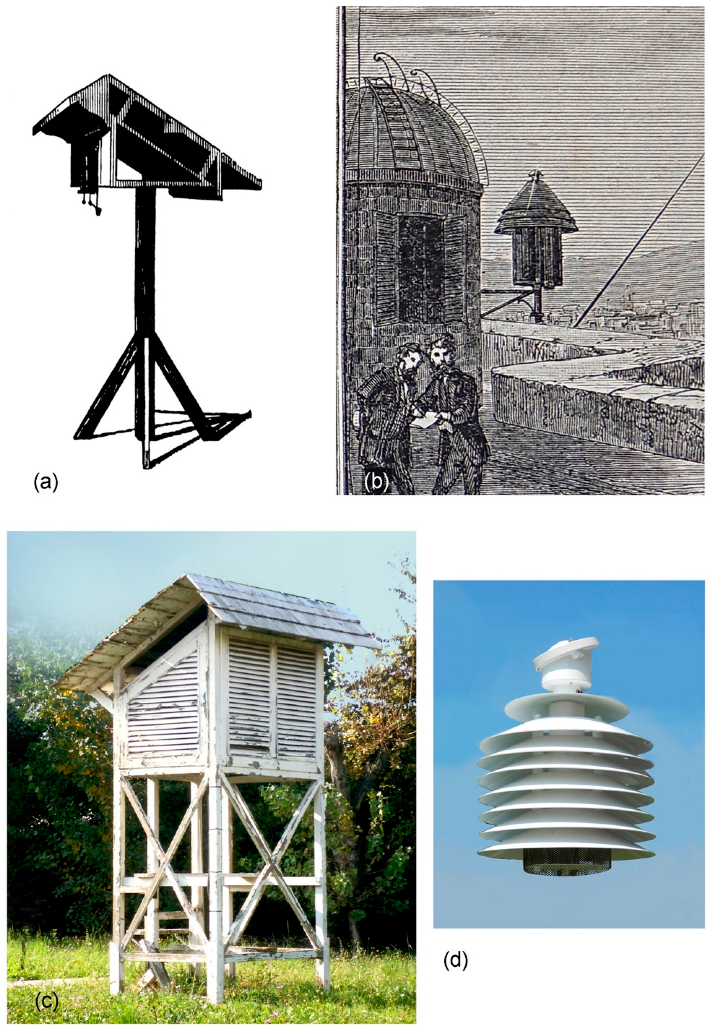
8. Exposure and Screens

8.1. Indoor or Outdoor Exposure

In the early period, thermometers were not screened from rain and radiation, except the LFTs, which were hung on the same wall, one on the northern side and one on the southern side, to investigate the impact of the southern and northern winds and the solar radiation [47,110]. Except this and some other cases, it is rare to find documentation of whether the thermometer was kept indoors or outdoors, because the exposure was considered obvious, and there was no need for specifying it. Sometimes, useful notes may be found, and the analysis of the data may clarify. Each observer, however, adopted personal solutions. For instance, from 1658 to 1670, Ismaël Boulliau adhered to the Medici Network, and the protocol required the thermometer exposed outside. However, he lived in Paris, in the city centre, at the ground floor of a building without private garden. He had the problem that, if the thermometer had been hung outside the window, it would have been stolen in no time. Therefore, his solution was to leave the house some ten minutes before the reading and keep the thermometer exposed until it reached equilibrium [49]. In the 18th century, most of the early thermometers were not weather resistant [34,50] and were used indoors, with the advantage of investigating the conditions where people lived. Thermometers were not weather resistant for two critical issues: (i) the capillary tube was fixed to the wooden tablet with an iron wire through narrow holes. Shrinkage of the wooden tablet decreased the wire tension and the capillary slipped with respect to the scale on the tablet; swelling increased the wire tension, breaking the capillary; (ii) often, scales were on a paper strip glued on the tablet, and marks and values were in ink, not resistant to humidity. Therefore, thermometers could not be exposed to rain, dew, fog, high humidity, sunshine and so on. When, in 1723, the Royal Society, London, established an international network, the thermometer was kept inside [111].

In Italy, the tradition established after Medici Network (active 1654–1670) of the thermometer being exposed outdoors was very strong. Conversely, the protocol of the Royal Society, London, required indoor measurements. In the 18th century, thermometers were not weatherproof and had to be kept indoors to be protected from rain and sunshine. This generated a series of hybrid solutions. The external thermometers were not in free positions far from buildings, but were located in niches or partially open environments, and were affected by the thermal inertia of the masonry walls. The internal thermometers were kept in well ventilated rooms, with windows open, or opened some time before each reading to obtain measurements representative of the outdoor air. For instance, Giovanni Poleni observed in Padua from 1725 to 1761 keeping the thermometer indoors, but he ventilated the room thoroughly, before each reading. Giovan Battista Morgagni also measured in Padua from 1740 to 1768, with a thermometer kept inside and another kept outside. Finally, Giuseppe Toaldo and Vincenzo Chiminello observed from 1777 to 1812 with the thermometer exposed outside of the astronomic tower [21]. The problem is to quantitatively assess to what extent an indoor or outdoor thermometer of the 18th century was representative of the actual outdoor temperature, as measured following the WMO recommendations.

The best way to recognize the building’s influence is to test how much the daily range T_max − T_min is reduced when comparing values outdoors with those indoors. However, this is only possible when two or more readings are taken per day. In the case of a single reading, or two readings taken at times that are not representative of the daily cycle, the only way is to look at the variability of the difference of temperature between two consecutive days [21].

For each of the above observers, and for the modern data of the Aeronautica Militare, the Italian Air Force (1951–1990), taken as a reference, an analysis has been made of how much the day-by-day variability was penalized by the thermal inertia of the building [21,107,112]. The method consists of calculating, over the calendar year, the difference between the mean temperature of the running day j and the previous day j − 1 and considering the variance of these departures, i.e., the larger the building influence, the smaller the variance (Figure 15). The record of the Italian Air Force, with the thermometer kept in a louvered Stevenson screen, shows the highest variance. The record by Toaldo, taken in the free air outside the tower, but close to the widow to read data from inside, has about half the variance of the Air Force data. The well-ventilated room of the indoor observations made by Poleni had similar characteristics to the outdoor ones made by Morgagni with an overly protected thermometer. For both Poleni and Morgagni’s outdoor measurements, the variance is about one tenth of that of the Air Force data. Finally, the indoor measurements by Morgagni show the most reduced variability. This poor variability is further reduced in winter, when the severe cold discouraged Morgagni from ventilating his room.

Another useful test to recognize indoor or outdoor readings consists of plotting the temperature of the snowy days (as discussed in Section 5.2 and Figure 4). If the thermometer was correctly exposed outside, the plot of the frequency of the snowy days includes negative and near zero temperatures. If the thermometer was kept inside, the peak of frequency is around a positive value (e.g., +5 °C that represents the normal indoor temperature of an unheated, manned building of northern Italy).

In the second half of the 18th century, the technology improved, and the thermometers became weather resistant. The thermometers of the network of the Societas Meteorologica Palatina, Mannheim [87] were located outside, in positions not reached by the solar radiation, and far from buildings. This was the recommendation, but the efficiency of the free ventilation and the proximity to the wall can be tested with an index representing the normalized daily range of temperature (NDRT) over the calendar year, which is the range of the daily cycle (T_max − T_min) observed in the EIR, divided by the range of the corresponding calendar day over the modern reference period. As the WMO standard procedure requires thermometers located outdoors, in a free space, NDRT = 1 when the thermometer was freely exposed outdoors, and adequately shielded form direct sunshine and precipitation. When NDRT < 1, the range is penalized (i.e., T_max lower and T_min higher) because the thermometer was kept too close to a wall (NDRT slightly less than 1), in a loggia (NDRT < 1), or indoors (NDRT << 1). Conversely, if the thermometer was not adequately shielded against solar radiation, T_max increases and NDRT > 1. An example of NDRT is shown in Figure 16, considering Beccari (observations from 1742 to 1765), and Matteucci (from 1787 to 1792) who measured at their homes in Bologna [56]. The NDRT index shows that Beccari measured correctly from April to October, and that, in the cold season, the daily cycle was penalized, being reduced to half of its normal cycle. This suggests that in winter the thermometer was kept in a semi-enclosed environment and the data variability was smoothed. NDRT suggests that Matteucci kept the thermometer in a narrow or semi-enclosed space, influenced by the building structures, which smoothed the temperature variability over the whole calendar year, but especially in winter, when the thermometer seems to have been kept indoors.

8.2. Stands and Screens

To the best of our knowledge, Toaldo was the first who realized that solar radiation caused a bias, and applied shields [21,34,112]. In 1780, he noted that, in summer, the thermometer was hit by solar radiation during the first measurement in the morning, and applied a piece of cardboard to screen it, as he wrote in the log of 30 June 1780. In 1785, Toaldo hung outside some thermometers exposed to free air, but ‘protected against harm from the sky’ [21,113], i.e., sheltered from rain and sunshine. This is the first documentation of screens in Italy.

In EIR, the situation is complex, and each observer must be considered as a separate case, because there was no standardization, and the protection adopted depended on the observer’s sensitivity. Middleton [23] suggested that screens started to be used after 1835. Böhm et al. [114] concluded that temperature records taken prior to 1860 could be affected by radiation bias. In 1874, the IMC recommended the use of screens [34,109], but it was too early to tell which was best. However, screens were normally used after 1874.

The earliest shelters [34] that were used around the half of the 19th century, were named ‘stands’ (Figure 17a) and constituted a wooden frame, where thermometers could be hung, and a small roof on the top to shield from rain, but without any lateral protection [115]. Screens against both radiation and rain became popular in the second half of the 19th century and were metal cylinders with a cap (Figure 17b), or wooden cages, and finally the louvered Stevenson screen [116] (Figure 17c). In the 20th century, Aitken developed the multi-plate radiation shield (Figure 17d), originally made of metal, and recently of plastics [34].

9. Overview of Data Recovery: From Original Readings to ‘Standardized’ Data

In the previous sections, some specific biases of temperature measurements, the related equations, and the procedure to correct them, have been presented and discussed. Since the problems encountered are numerous and rather complex, it is convenient to put them in the order in which they are to be addressed, to avoid the risk of concentrating on details and losing the logical flow of the overall methodology.

For the air thermometer (Figure 18a), the first question is whether it was a Stancari or Amontons type. If it was an Amontons, it is necessary to recover the pressure reading too, and correct them for gravity (latitude) and temperature. The correction for the level above the sea or the ground is not necessary, because both the thermometer and the barometer were kept at the same level. Then comes the correction for the different temperatures of the thermometer (e.g., 100 °C) and the barometer (e.g., 0 °C) during the upper calibration point. From here on, the corrections are the same, regardless of thermometer type, i.e., the transformation to °C; the transformation to the modern time frame in UTC + 1; the correction for indoor/outdoor readings; and the correction for irregular reading times.

For liquid-in-glass thermometers (Figure 18b), a key difference occurs between mercury and spirit. Unfortunately, the liquid is not always specified in most metadata. Mercury is the best, because it is linear. Spirit also is almost linear if the thermometer was calibrated by comparison with a mercury thermometer: although the expansion is not linear, the scale is composed of sub-intervals to reflect and compensate for the departures. Conversely, if the spirit thermometer was calibrated with ice and boiling water, it needs to be corrected for the non-linearity, and in summer, it underestimates the temperature by some 4–5 °C. If the thermometer scale does not reach 100 °C but is limited to 40 °C or 50 °C, this suggests that it was calibrated by comparison with a mercury thermometer and the bias for non-linearity is strongly reduced to within ±0.5 °C (Section 5.4).

10. Conclusions

This paper has made a fundamental distinction between data ‘rescue’ and data ‘recovery’. The former is applied when data are copied, digitized, and made available in image or electronic media, without changes or transformations. The latter is applied when early readings are rescued and deciphered; the arbitrary units of temperature are transformed in °C; and the local time, based on the apparent solar cycle, is transformed in UTC. In addition, the data are corrected for the early instruments, exposure, and observational protocol. Finally, data are homogenized and validated. At this stage, they constitute a recovered dataset ready to be used as input for climate studies.

The methodology is long, complex and requires a multidisciplinary approach, with a number of skills in various disciplines (e.g., history of science, palaeography, old languages, physics, astronomy, and climatology) rarely found in the same person, but easily combined with a team of experts. This paper aims to assist, either as a review or as a guide, to addressing these issues.

Some basic considerations of IMPROVE [21] are still relevant today, e.g., knowledge of the past is one of the keys to interpreting the present and forecasting the future. The answer is conditioned by the quality of our present information, and this gives rise to some further questions: Is our knowledge based on the best available data? Can we improve data quality? Can we learn more from the past by utilising new, unexploited data? Are we really utilising the best strategies to interpret available data? [22].

To date, a widespread international approach has been devoted to data rescue. However, the recovery of early instrumental series requires a huge and long-lasting effort for data rescue and conversion. This explains why only a limited number of early records has been so far recovered. This paper has been devoted to explaining the methodology in the hope of enticing and assisting young colleagues who want to tackle this fundamental issue, and increase the number of high-quality, early instrumental series available for climate studies.

References

1. WMO. Guidelines on Best Practices for Climate Data Rescue; WMO Publication No. 1182; World Meteorological Organization: Geneva, Switzerland, 2016; ISBN 978-92-63-11182-1. [Google Scholar]
2. Brönnimann, S.; Brugnara, Y.; Allan, R.J.; Brunet, M.; Compo, G.P.; Crouthamel, R.I.; Jones, P.D.; Jourdain, S.; Luterbacher, J.; Siegmund, P.; et al. A roadmap to climate data rescue services. Geosci. Data J. 2018, 5, 28–39. [Google Scholar] [CrossRef]
3. Slivinski, L.C.; Compo, G.P.; Whitaker, J.S.; Sardeshmukh, P.D.; Giese, B.S.; McColl, C.; Allan, R.; Yin, X.; Vose, R.; Titchner, H.; et al. Towards a more reliable historical reanalysis: Improvements for version 3 of the Twentieth Century Reanalysis system. Q. J. R. Meteorol. Soc. 2019, 145, 2876–2908. [Google Scholar] [CrossRef]
4. Slivinski, L.C.; Compo, G.P.; Sardeshmukh, P.D.; Whitaker, J.S.; McColl, C.; Allan, R.J.; Brohan, P.; Yin, X.; Smith, C.A.; Spencer, L.J.; et al. An evaluation of the performance of the 20th Century Reanalysis version 3. J. Clim. 2021, 34, 1417–1438. [Google Scholar] [CrossRef]
5. Muñoz-Sabater, J.; Dutra, E.; Agustí-Panareda, A.; Albergel, C.; Arduini, G.; Balsamo, G.; Boussetta, S.; Choulga, M.; Harrigan, S.; Hersbach, H.; et al. ERA5-Land: A state-of-the-art global reanalysis dataset for land applications. Earth Syst. Sci. Data 2021, 13, 4349–4383. [Google Scholar] [CrossRef]
6. Urban, A.; Di Napoli, C.; Cloke, H.L.; Kysely, J.; Pappenberger, F.; Sera, F.; Schneider, R.; Vicedo-Cabrera, A.M.; Acquaotta, F.; Ragettli, M.S.; et al. Evaluation of the ERA5 reanalysis-based Universal Thermal Climate Index on mortality data in Europe. Environ. Res. 2021, 8, 111227. [Google Scholar] [CrossRef] [PubMed]
7. Mistry, M.N.; Schneider, R.; Masselot, P.; Royé, D.; Armstrong, B.; Kyselý, J.; Orru, H.; Sera, F.; Tong, S.; Lavigne, É.; et al. Comparison of weather station and climate reanalysis data for modelling temperature-related mortality. Sci. Rep. 2022, 12, 5178. [Google Scholar] [CrossRef]
8. Burgdorf, A.-M.; Brönnimann, S.; Adamson, G.; Amano, T.; Aono, Y.; Barriopedro, D.; Bullon, T.; Camenisch, C.; Camuffo, D.; Daux, V.; et al. DOCU-CLIM: A global documentary climate dataset for climate reconstructions. Sci. Data 2023, 10, 402. [Google Scholar] [CrossRef]
9. Chimani, B.; Auer, I.; Prohom, M.; Nadbath, M.; Paul, A.; Rasol, D. Data rescue in selected countries in connection with the EUMETNET DARE activity. Geosci. Data J. 2022, 9, 187–200. [Google Scholar] [CrossRef]
10. Brönnimann, S.; Allan, R.; Ashcroft, L.; Baer, S.; Barriendos, M.; Brázdil, R.; Brugnara, Y.; Brunet, M.; Brunetti, M.; Chimani, B.; et al. Unlocking Pre-1850 instrumental meteorological records: A Global inventory. BAMS 2019, 100, ES389–ES413. [Google Scholar] [CrossRef]
11. Authority of the Meteorological Committee. Report of the Proceedings of the Meteorological Congress at Leipzig in 1783; Protocols and Appendices; Her Majesty’s Stationary Office: London, UK, 1873. [Google Scholar]
12. Authority of the Meteorological Committee. Report of the Proceedings of the Meteorological Congress at Vienna in 1783; Protocols and Appendices; Her Majesty’s Stationary Office: London, UK, 1874. [Google Scholar]
13. IMC. Report of the Second International Meteorological Congress at Rome, 1879; Her Majesty’s Stationary Office: London, UK, 1879. [Google Scholar]
14. IMC. Report of the International Meteorological Committee, Meeting in Berne, 1880; Her Majesty’s Stationary Office: London, UK, 1881. [Google Scholar]
15. IMC. Report of the Second Meeting of the International Meteorological Committee, Held at Copenhagen, 1882; Her Majesty’s Stationary Office: London, UK, 1883. [Google Scholar]
16. IMC. Report of the Third Meeting of the International Meteorological Committee Held at Paris, 1885; Her Majesty’s Stationary Office: London, UK, 1887. [Google Scholar]
17. IMC. Report of the Fourth Meeting of the International Meteorological Committee, Zürich, 1888; Her Majesty’s Stationary Office: London, UK, 1889. [Google Scholar]
18. IMC. Report of the International Meteorological Committee, Upsala, 1894; Appendix II: On the proposed International Meteorological Bureau. Remarks by H.H. Hildebrandsson; Her Majesty’s Stationary Office: London, UK, 1895. [Google Scholar]
19. Foken, T.; Beyrich, F.; Wulfmeyer, V. 1. Introduction to Atmospheric Measurements. In Springer Handbook of Atmospheric Measurements; Foken, T., Ed.; Springer: Cham, Switzerland, 2021; pp. 1–32. [Google Scholar]
20. Howard, D. One Hundred Years of International Cooperation in Meteorology (1873–1973): A Historical Review; WMO No. 345, IV Annexes; World Meteorological Organization: Geneva, Switzerland, 1973. [Google Scholar]
21. Camuffo, D.; Jones, P. (Eds.) Improved Understanding of Past Climatic Variability from Early Daily European Instrumental Sources; Kluwer Academic Publishers: Dordrecht, The Netherlands, 2002; p. 392. ISBN 978-94-010-0371-1. [Google Scholar] [CrossRef]
22. Camuffo, D.; Jones, P. Improved Understanding of Past Climatic Variability from Early Daily European Instrumental Sources—Guest Editorial. Clim. Chang. 2002, 53, 1–4. [Google Scholar] [CrossRef]
23. Middleton, K.W.E. A History of the Thermometer and Its Use in Meteorology; Hopkins: Baltimore, MD, USA, 1996; p. 249. [Google Scholar]
24. Borchi, E.; Macii, R. Termometri e Termoscopi; Tipografia Coppini: Florence, Italy, 1997. [Google Scholar]
25. Borchi, E.; Macii, R. Meteorologia a Firenze. Nascita ed Evoluzione; Pagnini: Florence, Italy, 2009. [Google Scholar]
26. Frisinger, H.H. The History of Meteorology: To 1800; American Meteorological Society: Boston, MA, USA, 1983. [Google Scholar]
27. Landsberg, H.E. Historic Weather Data and Early Meteorological Observations. In Paleoclimate Analysis and Modelling; Hecht, A.D., Ed.; Wiley: New York, NY, USA, 1985; pp. 27–70. [Google Scholar]
28. Kington, J. Observing and measuring the weather. In Climates of British Isles: Present Past and Future; Hulme, M., Barrow, E., Eds.; Routledge: London, UK, 1997; pp. 137–152. [Google Scholar]
29. Chang, H. Inventing Temperature. Measurement and Scientific Progress; Oxford University Press: Oxford, UK, 2004. [Google Scholar]
30. Brázdil, R.; Pfister, C.; Wanner, H.; von Storch, H.; Luterbacher, J. Historical climatology in Europe—The state-of-the-art. Clim. Chang. 2005, 70, 363–430. [Google Scholar] [CrossRef]
31. Brázdil, R.; Bělínová, M.; Dobrovolný, P.; Mikšovský, J.; Pišoft, P.; Řeznícková, L.; Štěpánek, P.; Valášek, H.; Zahradnícek, P. History of Weather and Climate in the Czech Lands, Vol. IX. Temperature and Precipitation Fluctuations in the Czech Lands during the Instrumental Period; Masarykova Univerzita: Brno, Czech Republic, 2012; p. 236. [Google Scholar]
32. Przybylak, R.; Majorowicz, J.; Brázdil, R.; Kejan, M. (Eds.) The Polish Climate in the European Context: An Historical Overview; Springer: Dordrecht, The Netherlands, 2010; p. 535. [Google Scholar] [CrossRef]
33. Benincasa, F.; De Vincenzi, M.; Fasano, G. Storia della Strumentazione Meteorologica, nella Cultura Occidentale; CNR-IBIMET: Florence, Italy, 2019; ISBN 978 88 8080 326 3. [Google Scholar]
34. Camuffo, D. Microclimate for Cultural Heritage—Measurement, Risk Assessment, Conservation, Restoration and Maintenance of Indoor and Outdoor Monuments, 3rd ed.; Elsevier: Amsterdam, The Netherlands; New York, NY, USA, 2019; p. 582. ISBN 978-0-444-64106-9. [Google Scholar] [CrossRef]
35. Philo of Byzantium. De Ingeniis Spiritualibus; Codex Latinus Monacensis 534 (Codex of the 14th Century); Bayerische Staatsbibliothek: Munich, Germany, 2nd or 3rd Century BC. [Google Scholar]
36. Heron of Alexandria. Spiritalia; Harleian Collection No. 5605; British Museum: London, UK, c.10–70 AD. [Google Scholar]
37. Commandino, F. Heronis Alexandrini Spiritalium Liber; A Federigo Commandino Urbinate, ex Graeco, Nuper in Latinum Conversus; Frisolini: Urbino, Italy, 1575. [Google Scholar]
38. Aleotti, G.B. Artifitiosi et Curiosi Moti Spiritali di Herrone; Baldini: Ferrara, Italy, 1589. [Google Scholar]
39. Giorgi, A. Spiritali di Herone Alessandrino Ridotti in Lingua Volgare da Alessandro Giorgi da Urbino; Ragusi: Urbino, Italy, 1592. [Google Scholar]
40. Della Porta, G.B. Magiae Naturalis Sive de Miraculis Rerum Naturalium Libri Viginti; Hempelius: Frankfurt, Germany, 1607. [Google Scholar]
41. Sanctorius, S. Commentaria in Artem Medicam; Pars 3, Coll. 229; Somasco: Venice, Italy, 1612. [Google Scholar]
42. Sanctorius, S. Commentaria in Primam fen Primi Libri Canonis Avicennae; Sarcina: Venice, Italy, 1625. [Google Scholar]
43. Fludd, R. Tractatus Secundus, de Naturae Simia seu Technica Macrocosmi Historia; Roetelii: Frankfurt, Germany, 1624. [Google Scholar]
44. Fludd, R. Philosophia Sacra & Vere Christiana seu Meteorologia Cosmica; Bryan: Frankfurt, Germany, 1626. [Google Scholar]
45. Fludd, R. Philosophia Moysaica in qua Sapientia et Scientia Creationis Explicantur; Ramazzeni: Gouda, The Netherlands, 1638. [Google Scholar]
46. Magalotti, L. Saggi di Naturali Esperienze Fatte nell’Accademia del Cimento; Cocchini: Florence, Italy, 1666. [Google Scholar]
47. Targioni Tozzetti, G. Notizie Degli Aggrandimenti delle Scienze Fisiche Accaduti in Toscana nel Corso di Anni LX del Secolo XVII; Tomo, I., Ed.; Bouchard: Florence, Italy, 1780. [Google Scholar]
48. Antinori, V. Notizie Istoriche Relative all’Accademia del Cimento; Tipografia Galileiana: Florence, Italy, 1841. [Google Scholar]
49. Camuffo, D.; della Valle, A.; Becherini, F.; Rousseau, D. The earliest temperature record in Paris, 1658–1660, by Ismaël Boulliau, and a comparison with the contemporary series of the Medici Network (1654–1670) in Florence. Clim. Chang. 2020, 162, 903–922. [Google Scholar] [CrossRef]
50. Camuffo, D.; Bertolin, C. The earliest temperature observations in the World: The Medici Network (1654–1670). Clim. Chang. 2012, 111, 335–363. [Google Scholar] [CrossRef]
51. Camuffo, D.; Bertolin, C. The earliest spirit-in-glass thermometer and a comparison between the earliest period of the Central England Temperature series and the instrumental observations of two Italian stations of the Medici Network, active 1654–1670. Weather 2012, 67, 206–209. [Google Scholar] [CrossRef]
52. Amontons, G. Discours sur Quelques Propriétés de l’Air & le Moyen d’en Connoître la Température Dans tous les Climats de la Terre; Mémoires de Mathématique et de Physique; Martin Coignard & Guerin: Paris, France, 1702; pp. 155–174. [Google Scholar]
53. Poleni, G. Johannis Poleni Miscellanea hoc Est: I Dissertatio de Barometris et Thermometris; Aloysium Pavinum: Venice, Italy, 1709. [Google Scholar]
54. Stancari, V.F. De Thermometro ab Amontonio Recens Inventis 1708; Letter to G.F. Maraldi, Dated 1708, Printed Posthumous in Schedae Mathematicae; Barbiroli Archigymnasium: Bologna, Italy, 1713; pp. 53–55. [Google Scholar]
55. Camuffo, D.; della Valle, A.; Bertolin, C.; Santorelli, E. The Stancari Air Thermometer and the 1715–1737 record in Bologna, Italy. Clim. Chang. 2016, 139, 623–636. [Google Scholar] [CrossRef]
56. Camuffo, D.; della Valle, A.; Bertolin, C.; Santorelli, E. Temperature observations in Bologna, Italy, from 1715 to 1815; a comparison with other contemporary series and an overview of three centuries of changing climate. Clim. Chang. 2017, 142, 7–22. [Google Scholar] [CrossRef]
57. Matsuo, T.; Sasyo, Y. Non-melting phenomena of snowflakes observed in subsaturated air below freezing level. J. Meteorol. Soc. Jpn. Ser. II 1981, 59, 26–32. [Google Scholar] [CrossRef]
58. Masih, I. Understanding Hydrological Variability for Improved Water Management in the Semiarid Karkheh Basin, Iran; CRC Press/Balkema: Leiden, The Netherlands, 2011. [Google Scholar]
59. O’Gorman, P.A. Contrasting responses of mean and extreme snowfall to climate change. Nature 2014, 512, 416–418. [Google Scholar] [CrossRef]
60. Camuffo, D.; Becherini, F.; della Valle, A. Daily temperature observations in Florence at the mid-eighteenth century: The Martini series (1756–1775). Clim. Chang. 2021, 164, 42. [Google Scholar] [CrossRef]
61. Huygens, C. Letter to Robert Moray, Dated 2 January 1665 in Oeuvres Complètes de Christiaan Huygens; Société Hollandaise des Sciences: The Hague, The Netherlands, 1893. [Google Scholar]
62. Renaldini, C. Philosophia Rationalis, Naturalis Atque Moralis; Frambotti: Padua, Italy, 1681. [Google Scholar]
63. Dalencé, J. Traittez des Barométre Thermométres et Notiométres ou Hygrométres; Wetstein: Amsterdam, The Netherlands, 1688. [Google Scholar]
64. Newton, I. Scala graduum caloris. Philos. Trans. 1701, 22, 824–829. [Google Scholar]
65. de La Hire, P. Journal des Observations de M. de la Hire pour l’année 1717. Observations météorologiques faites à l’Observatoire Royal pendant l’année 1715. Mem. Acad. R. Sci. Paris 1718, 1–4. [Google Scholar]
66. Fahrenheit, D.G. Experimenta et observationes de congelatione acquae in vacuo factae. Philos. Trans. 1724, 33, 78–84. [Google Scholar]
67. du Crest Martine, J.B. Description de la Méthode d’un Thermomètre Universel; Valleyre: Paris, France, 1741. [Google Scholar]
68. Celsius, A. Observationer om twänne beständiga grader på en thermometer (Observations on two persistent degrees on a thermometer), Kungliga Svenska Vetenskaps Akademiens Handlingar. Ann. R. Swed. Acad. Sci. 1742, 4, 197–205. [Google Scholar]
69. Martine, G. Essays Medical and Philosophical; Millar: London, UK, 1740. [Google Scholar]
70. Cotte, L. Traité de Météorologie: Contenant 1. l’histoire des Observations Météorologiques, 2. un Traité des Météores, 3. l’histoire & la Description du Baromètre, du Thermomètre & des Autres Instruments Météorologiques, 4. les Tables des Observations Météorologiques & Botanico-Météorologiques, 5. les Résultats des Tables & des Observations, 6. la Méthode Pour Faire les Observations Météorologiques; Imprimérie Royale: Paris, France, 1774; p. 635. [Google Scholar]
71. Camuffo, D. Key problems in early wine-spirit thermometers and the ‘True Réaumur’ thermometer. Clim. Chang. 2020, 163, 1083–1102. [Google Scholar] [CrossRef]
72. Toaldo, G. Emendazione de’ Barometri e de’ Termometri; Giornale d’Italia Spettante alla Scienza Naturale, e Principalmente all’agricoltura, alle Arti, ed al Commercio; Milocco: Venice, Italy, 1776. [Google Scholar]
73. Derham, W. Tables of barometrical altitudes at Zurich in Switzerland in the year 1708 observed by Dr JJ. Scheuchzer. Philos. Trans. 1709, 26, 342–366. [Google Scholar]
74. du Crest Martine, J.B. Kleine Schriften von den Thermometern und Barometern; Klett: Augsburg, Germany, 1765. [Google Scholar]
75. De Luc, J.A. Recherches sur les Modifications de l’atmosphère: Contenant l’histoire Critique du Baromètre et du Thermomètre, Tome I; Self-Published: Geneva, Switzerland, 1772. [Google Scholar]
76. van Swinden, J.H. Dissertation sur la Comparaison des Thermomètres; Rey: Amsterdam, The Netherlands, 1778. [Google Scholar]
77. Lambert, J.H. Pyrometrie, Oder vom Maaße des Feuers und der Wärme; Haude and Spener: Berlin/Heidelberg, Germany, 1779. [Google Scholar]
78. Gaussen, M. Dissertation sur le Thermomètre de Réaumur; Fuzier: Béziers, France, 1789. [Google Scholar]
79. Goubert, P. Recherches sur les Différences qui Existent Entre les Thermomètres de Mercure et ceux d’esprit-de-vin, et sur les Moyens d’y Remédier; Merigot: Paris, France, 1798. [Google Scholar]
80. Wildt, J.C.D. Neue Vergleichung des Quecksilber und Weingeist Thermometers, nach Beobachtungen und Berechnungen. Arch. Naturl. 1825, 6, 299–301. [Google Scholar]
81. De Reaumur, R.A.F. Règles pour construire des thermomètres dont les degrés soient comparables et qui donnent des idées d’un chaud et d’un froid qui puissent être rapportés à des mesures connues. Mem. Acad. R. Sci. Paris 1730, 452–457. [Google Scholar]
82. De Reaumur, R.A.F. Second mémoire sur la construction des thermomètres dont les degrés soient compatibles. Mem. Acad. R. Sci. Paris 1731, 250–296. [Google Scholar]
83. Nollet, J.A. Leçons de Physique Expérimentale; Guerin: Paris, France, 1748; Volume 4. [Google Scholar]
84. Nollet, J.A. L’Art des Experiences; Durand: Paris, France, 1770; Volume 3. [Google Scholar]
85. Talas, S. Thermometers in the eighteenth century: J.B. Micheli du Crest’s works and the cooperation with G.F. Brander. Nuncius 2002, 17, 475–496. [Google Scholar] [CrossRef]
86. Gauvin, J.F. The instrument that never was: Inventing, manufacturing, and branding Réaumur’s thermometer during the enlightenment. Ann. Sci. 2012, 69, 515–549. [Google Scholar] [CrossRef]
87. Hemmer, J.J. Descriptio instrumentorum meteorologicorum, tam eorum, quam Societas distribuit, quam quibus praeter haec Manheimii utitur. Tomus 1. In Ephemerides Societatis Meteorologicae Palatinae; Officina Novae Societatis Typographicae: Mannheim, Germany, 1781; pp. 59–90. [Google Scholar]
88. Camuffo, D.; della Valle, A. The Newton linseed oil thermometer: An evaluation of its departure from linearity. Weather 2017, 72, 84–85. [Google Scholar] [CrossRef]
89. Camuffo, D.; della Valle, A. A summer temperature bias in early alcohol thermometers. Clim. Chang. 2016, 138, 633–640. [Google Scholar] [CrossRef]
90. Cavendish, H.; Heberden, W.; Aubert, A.; Deluc, J.A.; Maskelyne, N.; Horsley, S.; Planta, J. The report of the Committee of the Royal Society to consider of the Best Method of Adjusting the Fixed Points of Thermometers; and the Precautions Necessary to be Used in Making Experiments with these Instruments. Philos. Trans. 1777, 67, 816–857. [Google Scholar]
91. Camuffo, D. Calibration and instrumental errors in early measurements of air temperature. Clim. Chang. 2002, 53, 297–330. [Google Scholar] [CrossRef]
92. Camuffo, D. Errors in early temperature series arising from changes in style of measuring time, sampling schedule and number of observations. Clim. Chang. 2002, 53, 331–354. [Google Scholar] [CrossRef]
93. Camuffo, D.; della Valle, A.; Becherini, F. From time frames to temperature bias in long temperature series. Clim. Chang. 2021, 165, 38. [Google Scholar] [CrossRef]
94. Toaldo, G. Tavola del Levare e Tramontare del sole a ore Oltramontane—Dichiarazione per l’orologio Oltramontano detto Anche alla Francese; Penada: Padua, Italy, 1789. [Google Scholar]
95. Toaldo, G. Delle Ore Oltramontane. In Giornale Astro Meteorologico; Storti: Venice, Italy, 1789; pp. 3–15. [Google Scholar]
96. Toaldo, G. Metodo Facile per Descrivere gli Orologi Solari; Storti: Venice, Italy, 1790. [Google Scholar]
97. Decree of the French Republic/Municipality of Padua. Tutti gli Orologi Sieno Regolati Secondo l’Orario Francese; Decree Dated 10 Pratile Year V of the French Republic, i.e., 29 May 1797. Annali della Libertà Padovana, Ossia Raccolta Completa di Tutte le Carte Pubblicate in Padova dal Giorno della sua Libertà; Brandolese: Padua, Italy, 1797; Volume 2, pp. 129–130. [Google Scholar]
98. Toaldo, G. Istruzione Popolare sull’Orologio Oltramontano, Ossia Francese. Tipografia del Seminario a Spese di P; Brandolese: Padua, Italy, 1797. [Google Scholar]
99. Müller, M. Equation of time-problem in astronomy. Acta Phys. Pol. A 1995, 88 (Suppl. S49), 1–18. [Google Scholar]
100. Menne, M.J.; Williams, C.N., Jr.; Vose, R.S. The US historical climatology network monthly temperature data, version 2. Bull. Am. Meteorol. Soc. 2009, 90, 993–1007. [Google Scholar] [CrossRef]
101. Rischard, M.; McKinnon, K.A.; Pillai, N. Bias correction in daily maximum and minimum temperature measurements through Gaussian process modelling. arXiv 2019, arXiv:1805.10214v2. [Google Scholar] [CrossRef]
102. Andrighetti, M.; Zardi, D.; de Franceschi, M. History and analysis of the temperature series of Verona (1769–2006). Meteorog. Atmos. Phys. 2009, 103, 267–277. [Google Scholar] [CrossRef]
103. Winkler, P. Revision and necessary correction of the long-term temperature series of Hohenpeissenberg, 1781–2006. Theor. Appl. Climatol. 2009, 98, 259–268. [Google Scholar] [CrossRef]
104. Camuffo, D.; Becherini, F.; della Valle, A. Temperature observations in Florence, Italy, after the end of the Medici Network (1654–1670): The Grifoni record (1751–1766). Clim. Chang. 2020, 162, 943–963. [Google Scholar] [CrossRef]
105. Brugnara, Y.; Pfister, L.; Villiger, L.; Rohr, C.; Isotta, F.A.; Brönnimann, S. Early instrumental meteorological observations in Switzerland: 1708–1873. Earth Syst. Sci. Data 2020, 12, 1179–1190. [Google Scholar] [CrossRef]
106. Brugnara, Y.; Flückiger, J.; Brönnimann, S. Instruments, procedures, processing, and analyses. In Swiss Early Instrumental Meteorological Series; Brönnimann, S., Ed.; Geographica Bernensia G96: Bern, Switzerland, 2020; pp. 17–32. [Google Scholar] [CrossRef]
107. Cocheo, C.; Camuffo, D. Corrections of systematic errors and data homogenisation in the Padova series (1725-today). Clim. Chang. 2002, 53, 77–100. [Google Scholar] [CrossRef]
108. Camuffo, D.; Bertolin, C. Recovery of the Early Period of Long Instrumental Time Series of Air Temperature in Padua, Italy (1716–2007). Phys. Chem. Earth 2012, 40–41, 23–31. [Google Scholar] [CrossRef]
109. Hann, M. Hours of observation. In Report of the Proceedings of the Meteorological Congress at Vienna; Stanford: London, UK, 1874; pp. 52–53. [Google Scholar]
110. Antinori, V. Archivio Meteorologico Centrale Italiano; Società Tipografica sulle Logge del Grano: Florence, Italy, 1858. [Google Scholar]
111. Jurin, J. Invitatio ad observationes Meteorologicas communi consilio instituendas a Jacobo Jurin M. D. Soc. Reg. Secr. et Colleg. Med. Lond. Socio. Philos. Trans. 1723, 379, 422–427. [Google Scholar]
112. Camuffo, D. History of the long series of the air temperature in Padova (1725-today). Clim. Chang. 2002, 53, 7–76. [Google Scholar] [CrossRef]
113. Toaldo, G. Delle qualità fisiche delle Plaghe. In Saggi Scientifici e Letterari dell’Accademia di Padova; Accademia: Padua, Italy, 1789; Voluem 2, pp. 121–143. [Google Scholar]
114. Böhm, R.; Jones, P.D.; Hiebl, J.; Brunetti, M.; Frank, D.; Maugeri, M. The early instrumental warm-bias: A solution for long Central European temperatures series 1760–2007. Clim. Chang. 2010, 101, 41–67. [Google Scholar] [CrossRef]
115. Negretti, E.; Zambra, J.W. Meteorological Instruments: Explanatory of Their Scientific Principles, Method of Construction, and Practical Utility; William and Strahams: London, UK, 1864. [Google Scholar]
116. Stevenson, T. New description of box for holding thermometers. J. Scott. Meteorol. Soc. 1864, 1, 122. [Google Scholar]
117. Flammarion, C. L’Atmosphère. Description des Grands Phenomènes de la Nature; Hachette: Paris, France, 1872. [Google Scholar]
Figure 1. Flow of the steps (and skills) required for: (a) data rescue, (b) data recovery. Recovery concerns early readings, written in obscure form and units, and transform them in a dataset satisfying all requirements for climate data. Symbols § 3 to § 7 indicate the next Section 3, Section 4, Section 5, Section 6 and Section 7 where these topics are discussed. The recovered dataset constitutes the input for climate studies. This paper is concerned with data recovery, i.e., the yellow box in (b), and stops at the cyan box of climate studies.
Climate 11 00178 g001
Figure 2. An example of turning points from the register by Morgagni, Padua, in January 1741. Column headings are day of the month (d); hour (h); barometer (B); Thermometer outside (Tout); Another (thermometer) inside (Tin); weather notes. Note on day 16; readings time 15 h from sunset (=10 h 15 min a.m.) Tout = 1 ¾ °R sotto (encircled blue, which means below). All subsequent values of that column should be intended negative, till day 19, readings time 21 h from sunset (=16 h 15 min) Tout = ¼ °R di sopra (encircled red, which means above). All subsequent values are positive.
Climate 11 00178 g002
Figure 3. Air thermometers. (a) Amontons [52]: the top of the capillary tube is open. The temperature was obtained by summing the reading of the mercury column of the thermometer with the mercury column of the barometer. (b) Expansion of the air pocket. Changes in temperature or pressure displaced a certain volume of mercury (Hg) that passed from the spherical bulb to the column. The changeable free surface area of Hg in the bulb determined different rises in the column. H: level of the Hg column above the free Hg surface in the spherical bulb. (c) Poleni [53]: cylindrical bulb. (d) Stancari [54]: the top of the capillary tube is sealed. (Sources: (a) Amontons [52]; (b) our drawing; (c) Poleni [53]; (d) Stancari [54]).
Climate 11 00178 g003
Figure 4. Number of times the log reports that it snowed, versus the temperature of the day, classified by temperature bins of 0.5 °C. (a) The plot of Petronio Matteucci (observations 1782–1792) is peaked around 0 °C, and confirms that the thermometer was kept outdoors. (b) The plot of Poleni (observations 1725–1761), who kept the thermometer indoors, is peaked around +5 °C.
Climate 11 00178 g004
Figure 5. Some of the most popular thermometric scales in use in the first half of the 18th century. The Latin numbers I to XV and the names of the thermometers have been rewritten at the bottom of the figure, to make them more easily readable. (From Martine [69]).
Climate 11 00178 g005
Figure 6. Calibration of Réaumur thermometers. Note: a pot of boiling water [E] and a wooden tub [d] of crushed ice; a large thermometer [F] dipped in the crushed ice together with a small one [C]; the capillary tubes of these thermometers and those on the box on the floor have some levels marked with silk threads; the long tube in the centre of the box is marked every 10° up to 80 °R. On the table, a serving stand holds some glass phials (one of them [A] is lying on the table) used for volumetric calibration (from Nollet [84]. Some figures not related to calibration have been removed. Courtesy of Gallica.bnf.fr/Bibliothèque nationale de France).
Climate 11 00178 g006
Figure 7. Bias of the alcohol thermometers. (a): Departure of ethyl alcohol form linearity, i.e., the difference between readings made with an alcohol thermometer calibrated at 0 °C and 100 °C and a mercury thermometer (red line). The secants joining 0 °C to 40 °C and 0 °C to 55 °C are reported. (b): Bias combining the non-linearity of alcohol and a two-point calibration. Red line: the calibration of the alcohol thermometer is made at 0 °C and 100 °C; magenta: the calibration is made by comparison with a mercury thermometer at 0 °C and 50 °C; blue: idem but at 0 °C and 40 °C. The black arrow in (a) is an example at 20 °C of how much the departure from linearity departs from the secant, which represents the bias for that specific calibration (b).
Climate 11 00178 g007
Figure 8. Time elapsed from sunset to the lower culmination of the Sun (i.e., local midnight). Calculations are reported for the winter and summer solstices, and the equinoxes. Italy lies in the latitude belt from around 37° to 47° North (curly bracket).
Climate 11 00178 g008
Figure 9. The equation-of-time (continuous black line) with the two components highlighted, i.e., the effect due to the ellipticity of the orbit (magenta dotted line) and the inclination of the Earth’s axis (blue dotted line).
Climate 11 00178 g009
Figure 10. Departure of the local solar time (i.e., sundials) from the modern official time UTC + 1 calculated for 22 Italian cities. The change of 1 h in summer for energy saving has not been considered. This causes 1 h additional shift. Note that some curves overlap each other, e.g. Florence, Bologna and Bolzano; Foggia and Messina; Aosta and Torino.
Climate 11 00178 g010
Figure 11. Difference of temperature from an hour and the next one in Florence, Italy, represented as a matrix with the calendar days in abscissa and the hours in ordinate (CET = UTC + 1). From Camuffo et al. [93], by courtesy of Springer Nature.
Climate 11 00178 g011
Figure 12. Departure between the average daily temperature calculated as the mean of all the readings over 24 h and the ancient use based on (Tmax + Tmin)/2. Example made with modern data of Padua. Dots: real daily averages (T24h) over the calendar year; blue histogram: average difference by months; bars: minimum and maximum departure in the month.
Climate 11 00178 g012
Figure 13. Departure from the 24 h average of daily means calculated over the calendar year from two or three reading times (RT), as indicated in each graph.
Climate 11 00178 g013
Figure 14. Distribution of the departures from the 24 h average when the mean is obtained from two or three readings. Each box reports the selected RT, the value of the related mean (µ), and the standard deviation ( σ ).
Climate 11 00178 g014
Figure 15. Variance of the difference between the mean temperature of consecutive days over the calendar year. Air Force: the reference series of the Aeronautica Militare. Toaldo: observations with the thermometer kept outside. Poleni: thermometer kept in a well-ventilated room. Morgagni out: thermometer kept outdoors but greatly influenced by the building masonry. Morgagni in: thermometer kept indoors, in a poorly ventilated room.
Climate 11 00178 g015
Figure 16. Normalized daily range of temperature (NDRT) for the temperature observations by Beccari and Matteucci in Bologna during the 18th century.
Climate 11 00178 g016
Figure 17. (a) Stand for thermometers, produced by Negretti and Zambra [115]. (b) Cylindrical metal shield topped with three metal cones hung in the free air to the turret of the Observatory, Paris [117]. (c) Stevenson screen with louvered wood walls. (d) Aitken multiplate radiation screen.
Climate 11 00178 g017
Figure 18. (a) Flow diagram of the methodology to recover EIR from air thermometers. (Air thermometer from Cotte [70]). (b) Flow diagram of the methodology to recover EIR from liquid-in-glass thermometers. (Spirit thermometer from Cotte [70]).
Climate 11 00178 g018