Trends in Extreme Precipitation Indices in Northwest Ethiopia: Comparative Analysis Using the Mann–Kendall and Innovative Trend Analysis Methods

Abstract

This study analyzed long-term extreme precipitation indices using 4 × 4 km gridded data obtained from the National Meteorological Agency of Ethiopia between 1981 and 2018. The study examined trends in extreme precipitation over three districts (Lay Gayint, Tach Gayint, and Simada) in the northwestern highlands of Ethiopia. Innovative Trend Analysis (ITA) and Mann–Kendall (MK) trend tests were used to study extreme precipitation trends. Based on the ITA result, the calculated values of nine indices (90% of the analyzed indices) showed significant increasing trends (p < 0.01) in Lay Gayint. In Tach Gayint, 70% (seven indices) showed significantly increasing trends at p < 0.01. On the other hand, 60% of the extreme indices showed significant downward trends (p < 0.01) in Simada. The MK test revealed that 30% of the extreme indices had significantly increasing trends (p < 0.01) in Lay Gayint. In Tach Gayint, 30% of the extreme indices showed significant increasing trends at p < 0.05, while 10% of the extreme indices exhibited significant increasing trends at p < 0.01. In Simada, 20% of the extreme indices showed significant increasing trends at p < 0.05. Overall, the results showed that the ITA method can identify a variety of significant trends that the MK test misses.

1. Introduction

Climate change has altered the circulation and distribution of water resources while increasing the likelihood of extreme disasters [1,2,3,4]. Precipitation is an important variable in local climate characteristics and a critical element of the global water cycle [5]. The recurrence of extreme precipitation events, such as droughts and floods, has a significant impact on human livelihoods and socioeconomic development [6,7,8]. Average global mean temperature has been rising since the pre-industrial period, with 2015–2019 being the warmest period since records began in 1850 [9]. Every 1 °C temperature rise increases the moisture holding capacity of the air by 7% [10]. An increase in humidity leads to heavier precipitation and increases the risk of flooding. Recent studies on global precipitation trends show an increase in the frequency of extreme events [11,12]. Climate-related events cause more than 70% of reported natural disasters worldwide, with most of these disasters being caused by extreme precipitation events of floods and droughts [13]. According to the World Meteorological Organization (WMO) [9], the weather in Africa in 2019 was characterized by steadily rising temperatures, and the negative effects of weather and climate extreme events were large. East Africa in particular is prone to severe climate extremes such as droughts and floods [7]. The climate of the Horn of Africa had changed abruptly from drought conditions in 2018 to floods and landslides in late 2019 [9].

Ethiopia is one of the East African countries facing climate-related risks, such as floods and droughts, caused by climate change and variability [14]. Several studies confirmed that Ethiopia’s economy and food security, which are largely based on rain-fed agriculture, are very sensitive to fluctuations in rainfall and extreme events [7,15]. According to Bezu [16], Ethiopia has experienced at least two catastrophic droughts per decade. This has had an impact on the country’s environment and natural resources. The tropical currents of the Pacific Ocean are the primary global climatic drivers for such severe events (i.e., floods and droughts) in Ethiopia [17]. In addition, changes in precipitation extremes in the country are influenced by local-scale climate controls [18,19].

The current study districts (Lay Gayint, Tach Gayint, and Simada) in the northwestern part of the country are among the drought-prone and food-insecure districts of the Amhara Region [20,21] These districts are classified as chronically food insecure because of their reliance on regularly receiving food aid [22,23]. The food insecurity of the area is mainly caused by rainfall variability and associated drought episodes.

Investigating daily precipitation extreme indices within the context of climate change and variability holds significant importance for multiple reasons. The knowledge gained from this study can prove valuable for policymakers in their efforts to manage floods, control runoff, and understand hydrological processes. This understanding can also help assess the risk of altered rainfall patterns, particularly those that arise from extreme rainfall events resulting from climate change [24,25,26] highlight the need for a more comprehensive comprehension of extreme rainfall variability to aid in water resource management, drought monitoring, and flood control. Additionally, Obada et al. [27] emphasize the critical role that scientific analysis of extreme rainfall and its evolution plays in implementing effective operational management and mitigating flood risks. Overall, studying daily precipitation extreme indices is a substantial contribution to our understanding of climate change and its environmental impacts.

There are many studies on rainfall patterns and trends in Ethiopia. For instance, Berhan et al. [28] performed a trend analysis for observed trends in climatic extremes at Choke Mountain and reported a significant decrease in total precipitation along with a decrease in wet extremes. A significant decrease in extreme climate indices was found in the semi-arid areas of western Tigray [28]. Most precipitation extreme indices considered in their study in the southern and southwestern parts of Ethiopia showed increasing trends [29]. According to Damtew et al. [30], most extreme climate indices decreased in the Awash River basin. The disparity in the findings of extreme precipitation trends in Ethiopia might be attributed to extremely variable topography features, data analysis methodologies utilized, time series data length, number of meteorological stations, data quality, and spatial coverage of the studied area.

In South-eastern Ethiopia, Degefu et al. [31] found a significant downward trend in the extreme precipitation indices for annual and seasonal timescales. Dendir and Birhanu [32] identified inconsistencies in the trend of extreme climate events in the Gurage Zone in Central Ethiopia. Esayas et al. [33] reported that very wet days showed a positive trend in the midlands and highlands of Southern Ethiopia. Gedefaw et al. [34] found significantly increasing trends in seasonal and annual precipitation in the Amhara Region. Geremew et al. [15] discovered that extreme rainfall trends in Enebsie Sar Midir district, central Ethiopian highlands, did not show a systematic pattern. Worku et al. [35] found decreasing trends in annual precipitation extremes in the southern parts of the Blue Nile basin. Terefe et al. [19] found clearly decreasing trends for most extreme precipitation indices in the Meki watershed of the central rift valley basin. In addition, Terefe et al. [19] found significant decreasing trends for most extreme precipitation indices in the same watershed (the Meki watershed of the central Rift Valley basin).

The Mann–Kendall (MK) test [36,37] is widely used to detect monotonic trends. It is well-known that the MK and MMK methods rely on several assumptions. Therefore, the validity of utilizing these methods and the results they generate is contingent upon adhering to these assumptions [38].

The MK trend test offers several advantages over parametric tests [24,25,26]. Firstly, it is a non-parametric test and does not make any assumptions about the distribution of the data, making it useful for analyzing data that may not follow a normal distribution. Secondly, the MK trend test is a robust test and is less sensitive to outliers and missing values than other trend tests, making it more reliable when analyzing data that may contain extreme values or noise. Lastly, the MK trend test can handle ties in the data, which are multiple data points having the same value, making it useful for analyzing data with repeated values. Although the MK test is widely used in hydrological trend analysis, studies have shown that the presence of autocorrelation could affect trend identification using the MK and Sen’s slope methods [39,40]. Some studies have used pre-whitening technique to remove autocorrelation from datasets [39,40]. However, several studies have shown that pre-whitening can remove some of the true trends and may be ineffective when serial correlation persists beyond the first-order autoregressive process and the sample size is large [41,42]. To address this problem, Sen [43] proposed the Innovative Trend Analysis (ITA) approach, which can solve the challenge of trend detection in autocorrelated time series data. Studies around the world have confirmed the reliability of the ITA method [2,44,45,46,47].

This paper is novel in its application and comparison of Sen’s innovative trend test with the Mann–Kendall test, despite the widespread use of ITA trend analysis in various regions worldwide. However, to our knowledge, only a few studies in Ethiopia have utilized ITA trend analysis, including one in the Amhara regional state [34], another in the Meki watershed of the central rift valley basin of Ethiopia [19], and a third in Addis Ababa [48]. In contrast, most studies that analyze hydro-climatological data for trend analysis in Ethiopia have used the MK test, t-test, and linear regression test. The paper highlights the potential benefits of using Sen’s innovative trend test, particularly in countries like Ethiopia where there may be limited research on the use of ITA trend analysis. Overall, comparing these trend analysis methods can provide valuable insights into the strengths and limitations of each approach, helping researchers choose the most appropriate method for their specific research context.

The aim of this study is to analyze trends of extreme precipitation events in Northwestern Ethiopia and covering the three food-insecure districts of Lay Gayint, Tach Gayint, and Simada. The specific objectives are: (i) to examine trends in extreme precipitation using the ITA and MK methods; and (2) to compare the results of the ITA method with the MK test.

2. Materials and Methods

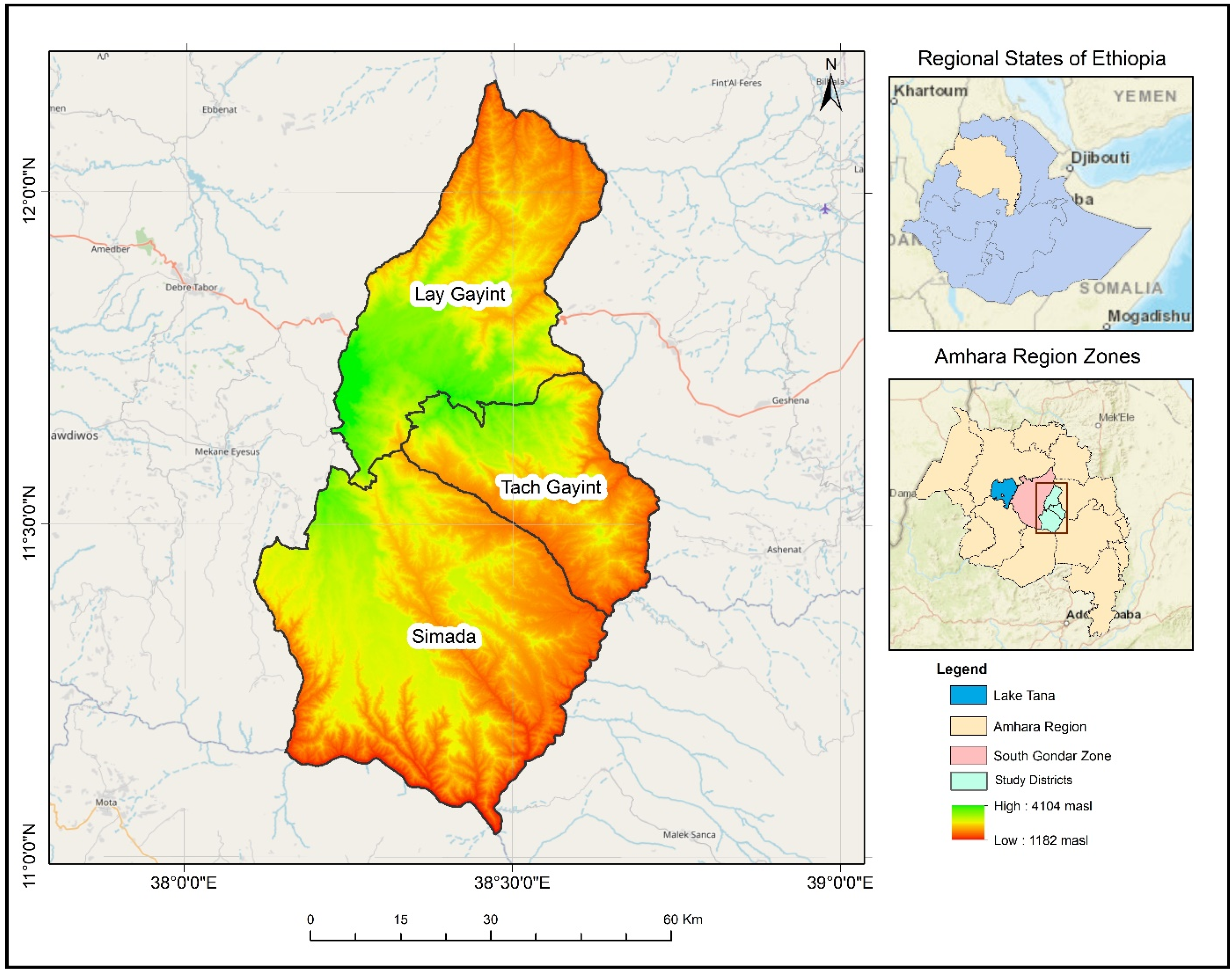
2.1. Study Area Description

The study area covers Tach Gayint, Lay Gayint, and Simada districts (Woredas in Amharic) in the South Gondar Administrative Zone of the Amhara National Regional State of Ethiopia (Figure 1). Lay Gayint is located in the High Dega agroecological zone (3200–3700 m a.s.l.), while Tach Gayint and Simada are located in Dega (2300–3200 m a.s.l.) and Woyna Dega (1500–2300 m a.s.l.), respectively [49]. Average annual rainfall ranges from 788 mm in Simada to 1096 mm in Lay Gayint, while the average annual temperature ranges from 14.4 °C in Lay Gayint to 18.2 °C in Simada. The main rainy season (Kiremt) lasts from June to mid-September, and the small rainy season (Belg) lasts from March to May [20]. The bimodal precipitation system allows for two harvest seasons (peak and off-season, known locally as Meher and Belg, respectively). However, the Belg harvest is hampered by the short, highly variable, and often insufficient rainy season [20]. The study area is generally food insecure due to a delayed start, early finish, and low Belg outputs. Most households struggle to produce enough food and rely heavily on the Productive Safety Nets Program (PSNP). The PSNP is a national program implemented in almost all areas that are vulnerable to persistent food insecurity, with support from development partners, to help the poor build assets, improve their living standards, and eventually become self-sufficient in terms of nutrition and resilience to shocks and stresses. According to information from the South Gondar Zone Administration Office, five districts, including the study area, benefit from the PSNP (Simada, Libokemkem, Lay Gayint, Ebnat, and Tach Gayint). Due to limited access to infrastructure, inadequate and inefficient agricultural marketing system, and limited access to institutional support services, non-agricultural livelihood activities are not well established in the study area.

2.2. Data Sources and Quality Control

The National Meteorological Agency (NMA) of Ethiopia provided the precipitation data used for the study, which covered the period from 1981 to 2018. It is a gridded dataset (4 × 4 km grid) obtained by merging station records with remote sensing-based estimates [50]. The satellite-based estimates are used to bridge temporal and spatial gaps in station records. The gridded dataset is particularly useful in data-sparse regions [51]. The dataset has been evaluated extensively and has demonstrated strong performance when evaluated at station locations across Ethiopia [51,52]. It also provides a homogeneous dataset [53] and is therefore recommended for climate analysis. The gridded dataset with a 4 × 4 km grid was chosen for analysis due to three reasons: (1) weather stations over the study area are scarce and do not cover all the study sites [51], (2) station datasets have many missing values [54], and (3) most stations are recently established and lack sufficient data records to support trend analysis [51,52,54].

Homogeneity testing of climate data is crucial in climatological research, particularly when evaluating climate change [55]. When weather stations record long-term series climate data, non-climatic factors of the data are inevitably influenced due to changes in instruments, observers, site locations, or surrounding environments [56]. In this study, the homogeneity of precipitation data was examined using the RHtests_dlyPrcp software, a tool developed in the R programming language for testing the homogeneity of daily precipitation data. The software is designed to identify and adjust for artificial shifts in climate data series caused by various factors unrelated to climate change. The tool utilizes statistical tests to detect the presence of inhomogeneities in the data. If significant inhomogeneities are detected, the tool can then adjust the data by eliminating the effects of non-climatic factors, allowing for a more precise analysis of climate trends. The RHtests_dlyPrcp package is commonly used in climatological research and has been documented in the literature [57]. In this study, the RHtests_dlyPrcp software indicated no significant inhomogeneities that necessitated mean adjustments. Hence, the original data series was used for further analysis.

2.3. Data Analysis

Extreme precipitation indices were calculated with the specially developed software RClimDex (version 1.0) [58] running under the programming environment R (http://www.rproject.org/ (accessed on 23 February 2023)). There are many extreme precipitation indices compiled by the Expert Team on Climate Change Detection and Indices (ETCCDI) [59]. Climate indices are easy to understand and are also statistically reliable quantitative indicators for climate extremes [60]. Based on the ETCCDI, 10 precipitation extreme indices were selected for the present study.

Table 1. Definition of the extreme precipitation indices used in the study.

Index	Indicator Name	Definition of the Index	Units
SDII	Simple daily intensity index	Annual total precipitation divided by the number of wet days	mm/day
Rx1day	Max 1-day precipitation amount	Monthly maximum 1-day precipitation	mm
Rx5day	Max 5-day precipitation amount	Monthly maximum consecutive 5-day precipitation	mm
R10mm	Number of heavy precipitation days	Annual count of days when PRCP ≥ 10 mm	Days
R20mm	Number of very heavy precipitation days	Annual count of days when PRCP ≥ 20 mm	Days
CDD	Consecutive dry days	Maximum number of consecutive days with RR < 1 mm	Days
CWD	Consecutive wet days	Maximum number of consecutive days with RR ≥ 1 mm	Days
R95p	Very wet days	Annual total PRCP when RR > 95th percentile	mm
R99p	Extremely wet days	Annual total PRCP when RR > 99th percentile	mm
PRCPTOT	Annual total wet-day precipitation	Annual total PRCP in wet days (RR ≥ 1 mm)	mm

presents the selected indices with their descriptions and units. The Mann–Kendall (MK), Modified Mann–Kendall (MMK), Sen’s slope (SS), and ITA (both the statistical and graphical techniques) were used to detect trends and magnitudes in precipitation extreme indices. The “trend change” package in RStudio version 4.2.1 was applied for the test statistics.

2.3.1. Mann–Kendall/Modified Mann–Kendall and Sen’s Slope Estimator

The Mann–Kendall (MK) Test

The Mann–Kendall (MK) test [36,37] was used to detect significant trends in time-series data [61,62]. The presence of serial autocorrelation often affects the detection of trends in time series data [63]. Hence, the lag-1 autocorrelation coefficient in the data series was| calculated and assessed at a 5% confidence level.

Equation (1) is used to compare the ordered x_i and x_j datasets in this test. The test involves sorting a x_i dataset up to i = 1…, n − 1 and a x_j dataset up to j = i + 1…, n before conducting the comparison.

$$\mathrm{sgn}\left(x_j-x_i\right)=\left\{\begin{array}{ccc}+1& \mathrm{if} & \left(x_j-x_i\right)>0\\ 0& \mathrm{if} & \left(x_j-x_i\right)=0\\ -1& \mathrm{if} & \left(x_j-x_i\right)<0\end{array}\right\}$$

(1)

Secondly, the MK test statistic S is calculated through Equation (2) below.

$$S=\sum _{i=1}^{n-1} \sum _{j=i+1}^n \mathrm{sgn}\left(x_j-x_i\right)$$

(2)

Equation (2) represents the assumed value of n, which corresponds to the total data for the basic period being analyzed (e.g., a month or a year). Moving on to Equation (3), it provides the vs. variance value for the S test statistic, considering a normal probability distribution with a mean of zero. Lastly, Equation (4) outlines the calculation process for the Z statistic.

$$V_S=\frac{n(n-1)(2n+5)}{18}$$

(3)

$$Z=\left\{\begin{array}{ccc}\frac{S-1}{V_S}\hfill & \mathrm{for}& S>0\\ 0\hfill & \mathrm{for}& S=0\\ \frac{S+1}{V_S}\hfill & \mathrm{for}& S<0\end{array}\right\}$$

(4)

When comparing the calculated Z value to the normal distribution value corresponding to the selected significance level, two possible outcomes emerge. Firstly, if the calculated Z value is below this normal distribution value, the null hypothesis holds true, indicating no trend in the analyzed time series. Conversely, if the calculated value exceeds this absolute value, a trend is present, and the direction of the trend can be determined. Specifically, a negative Z value indicates a decreasing trend, while a positive Z value indicates an increasing trend.

The Modified Mann–Kendall (MMK) Test

The modified Mann–Kendall (MMK) test was used for serially correlated data with a significant lag-1 autocorrelation coefficient using the variance correction method of [40]. The negative and positive values of the MK and MMK test statistics show decreasing and increasing trends, respectively [21]. This test calculates the corrected z value and adjusts the variance of the original MK test. In this method, the variance value in Equation (4) for the MK test should be calculated according to Equations (5) and (6) below.

$$V_S^{*}=V_S\frac{n}{n^{*}}$$

(5)

$$\frac{n}{n^{*}}=1+\frac{2}{n\left(n-1\right)\left(n-2\right)}\sum _{x=1}^{n-1} \left(n-x\right)\left(n-x-1\right)\left(n-x-n\right){\theta }_{x }$$

(6)

In the context of the MMK test, the autocorrelation function between sequence numbers of data, denoted as ${\theta }_{x }$, plays a crucial role as it influences the effective data number, n^∗, causing autocorrelation within the time series. Meanwhile, n represents the overall data number in the series. To determine the Z value of the MMK test, the variance value in Equation (4) is replaced with Vs^∗. Subsequently, trends are identified by comparing this newly calculated Z value with the standard Z value, following a similar approach to the MK method. The comparison is based on α significance levels.

The Sen’s slope (SS) estimator is used to estimate the magnitude of the trend [64,65]. Negative and positive values of SS indicate decreasing and increasing trends, respectively. The test statistic is determined using Equations (5) and (6):

$$SS=\mathrm{median}\left(\frac{Q_j-Q_i}{j-i}\right)i<j$$

(7)

$$S{S}_{\mathrm{medium} }=\left\{\begin{array}{c}S{S}_{\left(\frac{N+1}{2}\right)}; \mathrm{i}\mathrm{f} N \mathrm{i}\mathrm{s} \mathrm{o}\mathrm{d}\mathrm{d}\\ \frac{1}{2}\left[S{S}_{\left(\frac{N}{2}\right)}+S{S}_{\left(\frac{N+2}{2}\right)}\right]; \mathrm{i}\mathrm{f} N \mathrm{i}\mathrm{s} \mathrm{e}\mathrm{v}\mathrm{e}\mathrm{n}\end{array}\right.$$

(8)

where Q_j and Q_i are consecutive data series, and SS is the magnitude of the trend. When SS has a positive or negative value, it shows that the trend’s magnitude is increasing or decreasing.

2.3.2. Innovative Trend Analysis (ITA)

The ITA technique proposed by Sen [43] was also applied to detect trends in the precipitation time series. The ITA method is free from the assumptions of serial autocorrelation, normality, and record length.

Graphical Innovative Trend Assessment (G-ITA)

The G-ITA method is essential for identifying (1) non-monotonic trends, (2) monotonic trends, and (3) distributional changes in climate parameter values between the first and second halves of a time series [66].

In this method, the initial phase involves dividing time-series data into two equal parts and arranging each sub-series independently in ascending order. For instance, in the present study, there were 38 precipitation observations (1981–2018) in the time series. In the subsequent phase, the first half of the sub-series is placed on the X axis, and the second half is placed on the Y axis, as shown in Figure 2. If the data points are 1:1 above or below the bisecting line, there is an upward or downward trend in the time series Sen [43]. The presence of no trend is indicated when the data under study is collected on the 1:1 line. If the data points scatter on both sides of the 1:1 line, this indicates a non-monotonic trend [43,66].

Statistical Innovative Trend Assessment (S-ITA)

In the S-ITA method, the time series is divided into two equal halves and ordered in ascending order. According to Sen [67], the slope, S_m, can be determined using the arithmetic mean of the ordered two-parts as follows:

$$S_m=\frac{x_2-x_1}{(n/2)}$$

(9)

In this Equation, n stands for the number of observations, $x_2$ and $x_1$, respectively, represent the mean values of the second and first half. Here, $(n/2)$ is the time difference between the two halves. The trend direction, i.e., positive or negative, is derived based on the slope sign (+ or −). The probability density function (PDF) of the slope fits the normal distribution and the standard deviation of the slope can be represented as:

$${\sigma }_s=\frac{\sqrt[2]{2}}{\sqrt[n]{n}}\sigma \sqrt{1-}\rho {\overline{x}}_1{\overline{x}}_2$$

(10)

where $\left(\rho {\overline{x}}_1{\overline{x}}_2\right)$ is the cross-correlation between the arithmetic means of the two halves in ascending order. S_cri is the confidence limit of a standard normal PDF at α percent significance level, and Şen [67], suggested finding the (1 − α) percent confidence limits for the trend slope as follows:

$${\mathrm{C}\mathrm{L}}_{1-\alpha }=0\pm S_{cri}\times {\sigma }_S$$

(11)

where ${\sigma }_S$ is the calculated standard deviation of the slope, $S_m$, from Equation (1). The null hypothesis, ${\mathrm{H}}_0$ (there is no significant trend), is accepted if the calculated slope is within the upper and lower CL limits (Equation (11)), or an alternative hypothesis, ${\mathrm{H}}_{\mathrm{a}}$ (there is a significant trend) is concluded. Moreover, this study includes a flow chart outlining the methodologies employed (Figure 3).

3. Results

3.1. Trends in Precipitation Extremes

3.1.1. Simple Daily Intensity Index (SDII), Consecutive Dry Days (CDD), Consecutive Wet Days (CWD), and Annual Total Wet-Day Precipitation (PRCPTOT)

The trend in precipitation extremes from 1981 to 2018 as recorded by the MK/MMK test is summarized in

Table 2. The Mann–Kendall/Modified-Mann–Kendall trend test and Sen Slope values of the extreme indices (1981–2018).

Indices	Lay Gayint		Tach Gayint		Simada
	MK/MMK	SS	MK/MMK	SS	MK/MMK	SS
Rx1day	1.10	0.12	−0.55	−0.05	−1.53	−0.15
Rx5day	1.70	0.45	−0.12	−0.03	−1.25	−0.22
R10mm	2.96	0.46 **	2.33	0.31 *	1.10	0.12
R20mm	1.98	0.14 *	0.49	0.02	−0.75	−0.01
CDD	−0.74	−0.13	1.70	0.26	1.88	0.26 *
CWD	3.57	0.86 **	2.86	0.85 **	3.34	0.79 **
R95p	1.50	2.06	0.27	0.53	−1.00	−1.08
R99p	1.50	0.72	−0.59	−0.29	−1.23	−0.58
PRCPTOT	2.91	9.16 **	2.46	5.42*	0.65	1.70
SDII	2.47	0.04 *	2.35	0.03*	1.32	0.01

* and ** significant at α 0.05 and 0.01 level, respectively. Bold values indicate MMK test values (series with significant autocorrelation).

. The trend of the SDII showed a significantly increasing trend at a rate of 0.04 mm/day for Lay Gayint (p < 0.05). The rate of change in Tach Gayint was 0.03 mm/day (p < 0.05). CDD showed a significantly increasing trend (p < 0.05) at a rate of 0.26 days/year in Simada. The result suggests that a drier condition was observed in both Simada and Tach Gayint compared to Lay Gayint. In all districts, CWD showed a statistically significant increasing trend (p < 0.01). The rate of change was 0.86 mm/day for Lay Gayint, 0.85 mm/day for Tach Gayint, and 0.79 mm/day for Simada. In Lay Gayint, PRCPTOT showed a statistically significant upward trend (p < 0.01) at a rate of 9.16 mm/year. The rate of change in Tach Gayint was 5.42 mm/year at p < 0.05.

The trend of precipitation extremes using the ITA method is given in

Table 3. The innovative trend analysis results in precipitation extreme indices in Lay Gayint (1981–2018).

Indices	SITA	SSD	Correlation $\left(\mathit{\rho }{\overline{\mathit{x}}}_1{\overline{\mathit{x}}}_2\right)$	UCL/LCL Sig. (p < 0.05)	UCL/LCL Sig. (p < 0.01)
Rx1day	0.10 **	0.01	0.97	±0.03	±0.03
Rx5day	0.38 **	0.04	0.97	±0.07	±0.09
R10mm	0.44 **	0.04	0.92	±0.07	±0.09
R20mm	0.15 **	0.01	0.98	±0.02	±0.02
CDD	−0.21 **	0.03	0.98	±0.05	±0.07
CWD	0.72 **	0.04	0.97	±0.07	±0.09
R95p	2.21 **	0.15	0.99	±0.28	±0.37
R99p	0.78 **	0.08	0.97	±0.15	±0.20
PRCPTOT	7.70 **	0.72	0.92	±1.41	±1.85
SDII	0.05 **	0.00	0.95	±0.01	±0.01

** significant at α 0.05 level. UCL/LCL represent upper and lower confidence limits.

,

Table 4. The innovative trend analysis results in precipitation extreme indices in Tach Gayint (1981–2018).

Indices	SITA	SSD	Correlation $\left(\mathit{\rho }{\overline{\mathit{x}}}_1{\overline{\mathit{x}}}_2\right)$	UCL/LCL Sig. (p < 0.05)	UCL/LCL Sig. (p < 0.01)
Rx1day	−0.11 **	0.02	0.94	±0.04	±0.05
Rx5day	−0.01	0.05	0.92	±0.09	±0.12
R10mm	0.29 **	0.03	0.93	±0.05	±0.07
R20mm	0.04 **	0.01	0.97	±0.01	±0.01
CDD	0.33 **	0.02	0.98	±0.04	±0.05
CWD	0.59 **	0.06	0.94	±0.11	±0.15
R95p	0.97 **	0.17	0.96	±0.33	±0.44
R99p	−0.44 **	0.05	0.98	±0.11	±0.14
PRCPTOT	3.93 **	0.40	0.95	±0.79	±1.04
SDII	0.04 **	0.00	0.96	±0.00	±0.01

** significant at α 0.05 level. UCL/LCL represent upper and lower confidence limits.

and

Table 5. The innovative trend analysis results in precipitation extreme indices in Simada (1981–2018).

Indices	SITA	SSD	Correlation $\left(\mathit{\rho }{\overline{\mathit{x}}}_1{\overline{\mathit{x}}}_2\right)$	UCL/LCL Sig. (p < 0.05)	UCL/LCL Sig. (p < 0.01)
Rx1day	−0.17 **	0.01	0.98	±0.01	±0.02
Rx5day	−0.29 **	0.02	0.97	±0.04	±0.06
R10mm	−0.08 **	0.01	0.97	±0.02	±0.03
R20mm	−0.03 **	0.00	0.98	±0.01	±0.01
CDD	0.18 **	0.02	0.97	±0.05	±0.06
CWD	0.42 **	0.04	0.94	±0.09	±0.12
R95p	−1.29 **	0.13	0.97	±0.26	±0.34
R99p	−0.79 **	0.05	0.98	±0.09	±0.12
PRCPTOT	0.27	0.16	0.99	±0.31	±0.41
SDII	0.01	0.00	0.96	±0.01	±0.02

** significant at α 0.05 level. UCL/LCL represent upper and lower confidence limits.

. Results showed a statistically significant increasing SDII trend in Lay Gayint (0.05 mm/day) and Tach Gayint (0.04 mm/day) at p < 0.01. In Lay Gayint, CDD increased at a statistically significant rate of 0.33 days/year (p < 0.01). The corresponding value for Simada was 0.18 days/year (p < 0.01). On the other hand, CDD showed a statistically significant decreasing trend (p < 0.01) in Lay Gayint at a rate of 0.21 days/year. CWD showed a statistically significant decreasing trend at a rate of 0.72 days/year in Lay Gayint (p < 0.01).

The corresponding values for Tach Gayint and Simada were 0.59 days/year and 0.42 days/year, respectively (p < 0.01). A statistically significant increasing PRCPTOT trend was observed in Lay Gayint (7.70 mm/year) and Tach Gayint (3.93 mm/year) at p < 0.01. The result showed that some significant increasing trends masked by the MK/MMK test are detected with the ITA method; indicating the ITA’s ability to identify trends in time series. The increasing trend towards the extremes mentioned above can also be clearly seen from the scattered points that lie above the 1:1 line in the cartesian coordinate system (Figure 4, Figure 5 and Figure 6).

3.1.2. Number of Heavy (R10mm) and Very Heavy (R20mm) Precipitation Days

Based on analysis of the MK/MMK test, R10mm showed a statistically significant increasing trend in Lay Gayint (0.46 days/year) at p < 0.01 and Tach Gayint (0.31 days/year) at p < 0.05. Regarding the trend of R20mm, Lay Gayint showed a statistically significant increasing trend (p < 0.01) at a rate of 0.14 days/year (Table 2). According to ITA analysis, the trends of R10mm and R20mm showed statistically significant decreasing trends in Simada at a rate of 0.08 days/year and 0.03 days/year, respectively, at p < 0.01. On the other hand, the trend of R10mm showed a significantly increasing trend (p < 0.01) with rates of 0.44 days/year and 0.29 days/year in Lay Gayint and Tach Gayint, respectively. R20mm showed a significantly increasing trend (p < 0.01) at rates of 0.15 days/year in Lay Gayint and 0.04 days/year in Tach Gayint. The increase in R10mm and R20mm indicates potential risks related to soil erosion and flooding (Table 3, Table 4 and Table 5). As shown in Figure 4, Figure 5 and Figure 6, the scatter points for R10mm and R20mm values in Tach Gayint and Lay Gayint districts are above the 1:1 line. The trends in Simada are unclear.

3.1.3. Maximum 1-Day (Rx1day) and 5-Day (Rx5day) Precipitation

As indicated in Table 2, the results of the MK/MMK test analysis showed that the trends of Rx1day and Rx5day in Lay Gayint increased at rates of 0.12 mm/year and 0.45 mm/year, respectively, but the trends were not statistically significant. On the other hand, the values in Tach Gayint increased by 0.05 mm/year (Rx1day) and 0.03 mm/year (Rx5days) and in Tach Gayint by 0.15 mm/year (Rx1day) and 0.22 mm/year (Rx5days). In Simada, the trends were not statistically significant over the study period. ITA analysis showed that a statistically significant increasing trend of Rx5day was recorded in Lay Gayint (0.38 mm/year) at p < 0.01. Tach Gayint, on the other hand, showed a statistically significant decreasing trend in Rx1day at p < 0.01. In addition, the Rx1day and Rx5day values in Simada showed statistically significant decreasing trends at rates of 0.17 mm/year and 0.29 mm/year, respectively, at p < 0.01 (Table 3, Table 4 and Table 5). Further examination of the ITA graph showed inconsistent trends for Rx1day and Rx5day values. As a result, the scatter points lying above and below the 1:1 line in Lay Gayint and Simada indicate rising and falling trends, respectively. For Tach Gayint, the scatter points showed unclear trends (Figure 4, Figure 5 and Figure 6).

3.1.4. Very Wet Days (R95p) and Extremely Wet Days (R99p)

The trend of R95p using the MK/MMK test showed a tendency to increase at both Lay Gayint and Tach Gayint. The trend of R99p showed an increasing trend in Lay Gayint but a decreasing trend in both Tach Gayint and Simada over the study period. However, the observed trends were not statistically significant in either case (Table 2). In contrast, the ITA test showed that the trends of R95p (2.21 mm/year) and R99p (0.78 mm/year) had statistically significant increasing trends in Lay Gayint at p < 0.01. Statistically significant decreasing trends of R95p (1.29 mm/year) and R99p (0.79 mm/year) were observed in Simada at p < 0.01. In Tach Gayint, R95p and R99p showed statistically significant increasing and decreasing trends, respectively, at p < 0.01 (Table 3, Table 4 and Table 5). The finding supports the ability of the ITA method to identify masked trends in time-series data; several significant increasing trends that the MK/MMK test missed were detected using the ITA. As shown in Figure 4, Figure 5 and Figure 6, the scatter points in Lay Gayint and Simada fall above and below the 1:1 line, representing rising and falling trends, respectively. The scatter points in Tach Gayint district showed unclear trends.

3.2. Comparison of Trend Analysis Methods

The comparison between the trend detection results by the two methods, i.e., the MK and ITA tests, is shown in

Table 6. Comparisons of results of trend analysis of precipitation extremes by the MK and ITA methods (1981–2018).

Indices	Lay Gayint		Tach Gayint		Simada
	MK	ITA	MK	ITA	MK	ITA
Rx1day	No	Yes (++)	No	Yes (− −)	No	Yes (− −)
Rx5day	No	Yes (++)	No	No	No	Yes (− −)
R10mm	Yes (++)	Yes (++)	Yes (+)	Yes (++)	No	Yes (++)
R20mm	Yes (+)	Yes (++)	No	Yes (++)	No	Yes (− −)
CDD	No	Yes (− −)	No	Yes (++)	Yes (+)	Yes (++)
CWD	Yes (++)	Yes (++)	Yes (++)	Yes (++)	Yes (− −)	Yes (++)
R95p	No	Yes (++)	No	Yes (++)	No	Yes (− −)
R99p	No	Yes (++)	No	Yes (− −)	No	Yes (− −)
PRCPTOT	Yes (++)	Yes (++)	Yes (+)	Yes (++)	No	No
SDII	Yes (+)	Yes (++)	Yes (+)	Yes (++)	No	No

Yes (+) and Yes (−) indicate significant increasing and decreasing trends at 5% significance level (p < 0.05); Yes (++) and Yes (− −) indicate significant increasing and decreasing trends at 1% significance level (p < 0.01). No indicates non-significant result.

. It is shown that statistically significant increasing or decreasing trends are observed in 11 (37%) of the precipitation time series with the MK test. The ITA found a significantly increasing or decreasing trend in 27(90%) of the precipitation time series, indicating that a large number of significant trends are detected by the ITA method. Likewise, any statistically significant trend detected by the MK test is identified by the ITA. The ITA detects trends in 16 (53%) of the extreme rainfall index time series that the MK tests failed to do.

4. Discussions

The study investigated variations and trends in precipitation extremes. According to the ITA results, the CDD, CWD, PRCPTOT, SDII, R95p, R10mm, and R20mm exhibited statistically significant increasing trends in Tach Gayint, while the Rx1day and R99p showed statistically significant decreasing trends at p < 0.01. With the exception of CDD, all extreme precipitation indices in Lay Gayint exhibited statistically significant increasing trends at p < 0.01. In Simada, R10mm, CDD, and CWD exhibited statistically significant increasing trends, while R95p, R99p, R20mm, Rx1day, and Rx5day showed statistically significant decreasing trends. The MK test findings in Lay Gayint showed statistically significant increasing trends for R10mm, CWD, PRCPTOT, R20mm, and SDII at p < 0.05. The CWD, R10mm, PRCPTOT, and SDII in Tach Gayint showed statistically significant increasing trends at p < 0.01. On the other hand, only CDD and CWD showed statistically significant increasing trends in Simada at p < 0.05 and p < 0.01, respectively.

The significance of extreme precipitation indices in the study area can be attributed to differences in elevation. Specifically, the Lay Gayint district is situated in the High Dega agroecological zone, with an elevation ranging from 3200 to 3700 m above sea level. In contrast, the Tach Gayint and Simada districts are located in the Dega zone (2300–3200 m above sea level) and the Woyna Dega zone (1500–2300 m above sea level), respectively [49], as it is explained in the methodology section of this study. Agroecological zones are defined based on the interactions between climate, topography, and soil characteristics, and can provide a useful framework for understanding the spatial distribution of extreme precipitation events. Different agroecological zones can have different temperature and moisture regimes, which can affect the timing, intensity, and type of extreme precipitation events that occur. This indicates that variations in elevation play a significant role in the spatial distribution of precipitation extremes. Previous research studies consistently demonstrate a strong correlation between elevation in Ethiopia and the spatial variability of precipitation extremes [7,19,28,68,69]. Overall, the study highlights the importance of considering elevation and agroecological zones when studying extreme precipitation events in the study area. The differences in elevation between the districts can lead to variations in the spatial distribution of extreme precipitation indices, which can have important implications for water resource management and disaster risk reduction.

The trend results we found for some extreme precipitation indices are similar to findings reported in previous studies [19,33,35,69]. Terefe et al. [19] reported the existence of statistically significant increasing trends for R10 mm and R20 mm in the Ejersalele and Tora stations in the Meki watershed, central Ethiopia. Similarly, increasing trends of R10 mm and R20 mm were reported by Esayas et al. [33], Shawul and Chakma [69], and Worku et al. [35] in the majority of weather stations in Southern Ethiopia, in the Upper Awash basin and Jemma Sub-basin of Ethiopia, respectively. Furthermore, studies by Damtew et al. [30], Degefu et al. [31], and Geremew et al. [15] found increasing trends of CWD and CDD in the Awash River basin and Southeastern and Northwestern Ethiopia, respectively. On the other hand, our results did not agree with the findings of some other studies. For example, a study by Esayas et al. [33] found statistically significant decreasing trend in CWD in Southern Ethiopia. The trend in PRCPTOT showed a statistically non-significant decreasing trend in the Jemma Sub-Basin of the Upper Blue Nile Basin [35]. Statistically non-significant decreasing trends in the Rx1day and Rx5day precipitation were observed in most of the studied agroecologies in the Gurage Zone, Southern Ethiopia [32]. Esayas et al. [33] reported that lowland and midland agroecologies in the Wolaita Zone of Southern Ethiopia exhibited statistically non-significant increasing trends for Rx1-day and Rx5-day. In general, topography, variations in record lengths, number of stations, and method of data analysis used account for the majority of observed discrepancies [7,68,70].

Comparison of the ITA and MK trend detection methods indicates that the ITA method is superior to the MK test. The ITA method detected statistically significant increasing and decreasing trends in 27 (90%) of the precipitation time series, which indicated that a large number of significant trends that were missed by the MK test were detected using the ITA method. The ITA method detected trends in 16 (53%) of the precipitation extreme time series that the MK tests did not detect. Singh et al. [71] compared the ITA with the MK test for assessing spatiotemporal variations of precipitation extremes in India and recommended the ITA as the better option. Harka et al. [72] found the ITA approach to be more reliable than the MK test in their study on the Wabe Shebelle River Basin of Ethiopia. Similarly, in their investigation of seasonal and annual rainfall variability in the Amhara Regional State, Gedefaw et al. [34] reported that the ITA was preferable to the MK test.

Several studies also noted the ITA method and its capacity to detect trends more effectively than the MK test in different parts of the world [2,10,73,74]. The ITA approach enables more in-depth interpretations of trend identification, which is advantageous for detecting trends that are hidden from view as well as for illustrating the trend variability of extreme events in a graphical form [45,47,75]. It illustrates monotonic and non-monotonic trends [2,43].

In general, the results provided useful information for policy makers and water resource managers, given that extreme precipitation events can result in natural disasters such as flooding and landslides. These events can cause significant damage to infrastructure and pose a threat to communities, thereby warranting careful and strategic management of water resources. There are several ways in which policy makers and water resource managers can prepare for extreme precipitation events, including developing early warning systems, building and maintaining infrastructure, implementing land-use planning and zoning, promoting sustainable agriculture, educating and training communities, and investing in research. By implementing these strategies, policy makers and water resource managers can help reduce the risk and impact of extreme precipitation events and promote the safety and well-being of communities.

Although the study may have identified long-term trends in extreme precipitation indices in the study area, it may not have explored the underlying causes of these trends. Therefore, future investigations could focus on examining the meteorological, climatological, and environmental factors that contribute to changes in extreme precipitation. Additionally, while the study may have focused on three districts of Northwest Ethiopia (Lay Gayint, Tach Gayint, and Simada), expanding the analysis to other districts could help identify spatial patterns in extreme precipitation indices and vulnerable regions. Furthermore, while the study may have focused on the trends in extreme precipitation indices themselves, future investigations could examine the impacts of these events on the environment, agriculture, infrastructure, and communities in the area. Such research could help inform adaptation and mitigation strategies to reduce the negative impacts of extreme precipitation events. Finally, investigating the potential for future changes in extreme precipitation could be valuable. Although the study may have analyzed trends in extreme precipitation indices over a historical period, using climate models to project how these trends may change in the future under different scenarios of greenhouse gas emissions and climate change could help inform planning and decision-making for future climate risks and impacts in the study area.

5. Conclusions

The study conducted an analysis of the frequency and intensity of extreme precipitation events in Northwest Ethiopia using both the MK/MMK methods. The findings revealed significant changes in the patterns of extreme precipitation events in the area over the past few decades, with an increase in both frequency and intensity. It is noteworthy that trend detection studies in the literature typically rely on both the MK/MMK test and the SS investigation. While the MK/MMK test determines the existence of a trend and its direction, the trend magnitude is calculated using the SS method only if a significant trend is found according to these methodologies. Otherwise, the SS method is generally not employed. It is worth noting that the validity of the results obtained from the MK/MMK methods is subject to several assumptions. The study also compared the MK/MMK and SS methodologies with the ITA method, another popular trend detection tool. Although the different methodologies resulted in some variations in trend magnitudes, the ITA and SS methods’ trend direction results matched up in some extreme precipitation indices. The ITA method provides graphical and statistical trend analysis that objectively interprets the trends. Another significant finding of the study is that neither the SS nor the ITA methods rely on assumptions or statistical significance levels. Therefore, employing and comparing different methods such as MK/MMK, SS, and ITA for trend analysis can provide more detailed information on trend identification in the studied data. This can ultimately lead to more accurate climate analysis and better-informed decision-making. By using multiple methodologies, researchers can gain a comprehensive understanding of trends and minimize the impact of potential bias resulting from a single method.

References

1. Mukherjee, S.; Mishra, A.K. Cascading effect of meteorological forcing on extreme precipitation events: Role of atmospheric rivers in southeastern US. J. Hydrol. 2021, 601, 126641. [Google Scholar] [CrossRef]
2. Wang, Y.; Xu, Y.; Tabari, H.; Wang, J.; Wang, Q.; Song, S.; Hu, Z. Innovative trend analysis of annual and seasonal rainfall in the Yangtze River Delta, eastern China. Atmos. Res. 2020, 231, 104673. [Google Scholar] [CrossRef]
3. Yang, Y.; Gao, M.; Xie, N.; Gao, Z. Relating anomalous large-scale atmospheric circulation patterns to temperature and precipitation anomalies in the East Asian monsoon region. Atmos. Res. 2020, 232, 104679. [Google Scholar] [CrossRef]
4. Marie, M.; Yirga, F.; Haile, M.; Tquabo, F. Farmers’ choices and factors affecting adoption of climate change adaptation strategies: Evidence from northwestern Ethiopia. Heliyon 2020, 6, e03867. [Google Scholar] [CrossRef]
5. Jin, H.; Chen, X.; Wu, P.; Song, C.; Xia, W. Evaluation of spatial-temporal distribution of precipitation in mainland China by statistic and clustering methods. Atmos. Res. 2021, 262, 105772. [Google Scholar] [CrossRef]
6. Ferijal, T.; Batelaan, O.; Shanafield, M. Rainy season drought severity trend analysis of the Indonesian maritime continent. Int. J. Climatol. 2021, 41, E2194–E2210. [Google Scholar] [CrossRef]
7. Gebrechorkos, S.H.; Hülsmann, S.; Bernhofer, C. Changes in temperature and precipitation extremes in Ethiopia, Kenya, and Tanzania. Int. J. Climatol. 2019, 39, 18–30. [Google Scholar] [CrossRef] [Green Version]
8. Janizadeh, S.; Pal, S.C.; Saha, A.; Chowdhuri, I.; Ahmadi, K.; Mirzaei, S.; Mosavi, A.H.; Tiefenbacher, J.P. Mapping the spatial and temporal variability of flood hazard affected by climate and land-use changes in the future. J. Environ. Manag. 2021, 298, 113551. [Google Scholar] [CrossRef]
9. World Meteorological Organization (WMO). State of the Climate in Africa 2020; World Meteorological Organization: Geneva, Switzerland, 2021. [Google Scholar]
10. Marak, J.D.K.; Sarma, A.K.; Bhattacharjya, R.K. Innovative trend analysis of spatial and temporal rainfall variations in Umiam and Umtru watersheds in Meghalaya, India. Theor. Appl. Climatol. 2020, 142, 1397–1412. [Google Scholar] [CrossRef]
11. Myhre, G.; Alterskjær, K.; Stjern, C.W.; Hodnebrog, Ø.; Marelle, L.; Samset, B.H.; Sillmann, J.; Schaller, N.; Fischer, E.; Schulz, M.; et al. Frequency of extreme precipitation increases extensively with event rareness under global warming. Sci. Rep. 2019, 9, 16063. [Google Scholar] [CrossRef] [Green Version]
12. Papalexiou, S.M.; Montanari, A. Global and Regional Increase of Precipitation Extremes Under Global Warming. Water Resour. Res. 2019, 55, 4901–4914. [Google Scholar] [CrossRef]
13. Wang, Y.; Liu, G.; Guo, E. Spatial distribution and temporal variation of drought in Inner Mongolia during 1901–2014 using Standardized Precipitation Evapotranspiration Index. Sci. Total Environ. 2019, 654, 850–862. [Google Scholar] [CrossRef] [PubMed]
14. Gezie, M. Farmer’s response to climate change and variability in Ethiopia: A review. Cogent Food Agric. 2019, 5, 1613770. [Google Scholar] [CrossRef]
15. Geremew, G.M.; Mini, S.; Abegaz, A. Spatiotemporal variability and trends in rainfall extremes in Enebsie Sar Midir district, northwest Ethiopia. Model. Earth Syst. Environ. 2020, 6, 1177–1187. [Google Scholar] [CrossRef]
16. Bezu, A. Analyzing Impacts of Climate Variability and Changes in Ethiopia: A Review. Am. J. Mod. Energy 2020, 6, 65. [Google Scholar] [CrossRef]
17. Nicholson, S.E. Climate and climatic variability of rainfall over eastern Africa. Rev. Geophys. 2017, 55, 590–635. [Google Scholar] [CrossRef] [Green Version]
18. Gebrehiwot, B.; Gessesse, B.; Melgani, F. Characterizing the spatiotemporal distribution of meteorological drought as a response to climate variability: The case of rift valley lakes basin of Ethiopia. Weather. Clim. Extrem. 2019, 26, 100237. [Google Scholar] [CrossRef]
19. Terefe, S.; Bantider, A.; Teferi, E.; Abi, M. Spatiotemporal trends in mean and extreme climate variables over 1981–2020 in Meki watershed of central rift valley basin, Ethiopia. Heliyon 2022, 8, e11684. [Google Scholar] [CrossRef]
20. Endalew, H.A.; Sen, S. Effects of climate shocks on Ethiopian rural households: An integrated livelihood vulnerability approach. J. Environ. Plan. Manag. 2020, 64, 399–431. [Google Scholar] [CrossRef]
21. Likinaw, A.; Alemayehu, A.; Bewket, W. Local-scale climate variability and trends in a vulnerable rural landscape, northwest Ethiopia. Malays. J. Trop. Geogr. 2022, 48, 19–44. [Google Scholar]
22. Bazezew, A.; Bewket, W.; Nicolau, M. Rural households’ livelihood assets, strategies and outcomes in drought-prone areas of the Amhara Region, Ethiopia: Case Study in Lay Gaint District. Afr. J. Agric. Res. 2013, 8, 5716–5727. [Google Scholar] [CrossRef]
23. Tizazu, G.Z. Food Security Status of Rural Households in Lay Gayint Woreda of South Gondar Zone, Amhara Region, Ethiopia. Int. J. African Asian Stud. 2019, 57, 12–26. [Google Scholar] [CrossRef] [Green Version]
24. Srivastava, P.K.; Pradhan, R.K.; Petropoulos, G.P.; Pandey, V.; Gupta, M.; Yaduvanshi, A.; Jaafar, W.Z.W.; Mall, R.K.; Sahai, A.K. Long-term trend analysis of precipitation and extreme events over Kosi River Basin in India. Water 2021, 13, 1695. [Google Scholar] [CrossRef]
25. Vondou, D.A.; Guenang, G.M.; Djiotang, T.L.A.; Kamsu-Tamo, P.H. Trends and interannual variability of extreme rainfall indices over Cameroon. Sustainability 2021, 13, 6803. [Google Scholar] [CrossRef]
26. Salameh, A.A.M.; Ojeda, M.G.-V.; Esteban-Parra, M.J.; Castro-Díez, Y.; Gámiz-Fortis, S.R. Extreme rainfall indices in southern levant and related large-scale atmospheric circulation patterns: A spatial and temporal analysis. Water 2022, 14, 3799. [Google Scholar] [CrossRef]
27. Obada, E.; Alamou, E.A.; Biao, E.I.; Zandagba, E.B.J. Interannual variability and trends of extreme rainfall indices over Benin. Climate 2021, 9, 160. [Google Scholar] [CrossRef]
28. Berhane, A.; Hadgu, G.; Worku, W.; Abrha, B. Trends in extreme temperature and rainfall indices in the semi-arid areas of Western Tigray, Ethiopia. Environ. Syst. Res. 2020, 9, 1–20. [Google Scholar] [CrossRef] [Green Version]
29. Beyene, T.K.; Jain, M.K.; Yadav, B.K.; Agarwal, A. Multiscale investigation of precipitation extremes over Ethiopia and teleconnections to large-scale climate anomalies. Stoch. Environ. Res. Risk Assess. 2022, 36, 1503–1519. [Google Scholar] [CrossRef]
30. Damtew, A.; Teferi, E.; Ongoma, V.; Mumo, R.; Esayas, B. Spatiotemporal Changes in Mean and Extreme Climate: Farmers’ Perception and Its Agricultural Implications in Awash River Basin, Ethiopia. Climate 2022, 10, 89. [Google Scholar] [CrossRef]
31. Degefu, M.A.; Tadesse, Y.; Bewket, W. Observed changes in rainfall amount and extreme events in southeastern Ethiopia, 1955–2015. Theor Appl Clim. 2021, 144, 967–983. [Google Scholar] [CrossRef]
32. Dendir, Z.; Birhanu, B.S. Analysis of Observed Trends in Daily Temperature and Precipitation Extremes in Different Agroecologies of Gurage Zone, Southern Ethiopia. Adv. Meteorol. 2022, 2022. [Google Scholar] [CrossRef]
33. Esayas, B.; Simane, B.; Teferi, E.; Ongoma, V.; Tefera, N. Trends in extreme climate events over three agroecological zones of Southern Ethiopia. Adv. Meteorol. 2018, 2018, 1–17. [Google Scholar] [CrossRef]
34. Gedefaw, M.; Yan, D.; Wang, H.; Qin, T.; Girma, A.; Abiyu, A.; Batsuren, D. Innovative trend analysis of annual and seasonal rainfall variability in Amhara Regional State, Ethiopia. Atmosphere 2018, 9, 326. [Google Scholar] [CrossRef] [Green Version]
35. Worku, G.; Teferi, E.; Bantider, A.; Dile, Y.T. Observed changes in extremes of daily rainfall and temperature in Jemma Sub-Basin, Upper Blue Nile Basin, Ethiopia. Theor. Appl. Climatol. 2019, 135, 839–854. [Google Scholar] [CrossRef]
36. Kendall, M.G. Rank Correlation Methods, 4th ed.; Charles Griffin & Company Limited: London, UK, 1975. [Google Scholar]
37. Mann, H.B. Nonparametric tests against trend. Econom. J. Econom. Soc. 1945, 13, 245–259. [Google Scholar] [CrossRef]
38. Birpınar, M.E.; Kızılöz, B.; Şişman, E. Classic trend analysis methods’ paradoxical results and innovative trend analysis methodology with percentile ranges. Theor. Appl. Climatol. 2023, 153, 1–8. [Google Scholar] [CrossRef]
39. Hamed, K.H.; Ramachandra Rao, A. A modified Mann-Kendall trend test for autocorrelated data. J. Hydrol. 1998, 204, 182–196. [Google Scholar] [CrossRef]
40. Yue, S.; Pilon, P.; Phinney, B.; Cavadias, G. The influence of autocorrelation on the ability to detect trend in hydrological series. Hydrol. Process 2002, 16, 1807–1829. [Google Scholar] [CrossRef]
41. Kumar, S.; Merwade, V.; Kam, J.; Thurner, K. Streamflow trends in Indiana: Effects of long term persistence, precipitation and subsurface drains. J. Hydrol. 2009, 374, 171–183. [Google Scholar] [CrossRef]
42. Yue, S.; Wang, C.Y. The Mann-Kendall test modified by effective sample size to detect trend in serially correlated hydrological series. Water Resour. Manag. 2004, 18, 201–218. [Google Scholar] [CrossRef]
43. Şen, Z. Innovative Trend Analysis Methodology. J. Hydrol. Eng. 2012, 17, 1042–1046. [Google Scholar] [CrossRef]
44. Şïşman, E.; Kizilöz, B.; Bïrpinar, M.E. Trend slope risk charts (TSRC) for piecewise ITA method: An application in Oxford, 1771–2020. Theor. Appl. Climatol. 2022, 150, 863–879. [Google Scholar] [CrossRef]
45. Caloiero, T. Evaluation of rainfall trends in the South Island of New Zealand through the innovative trend analysis (ITA). Theor. Appl. Climatol. 2020, 139, 493–504. [Google Scholar] [CrossRef]
46. Serencam, U. Innovative trend analysis of total annual rainfall and temperature variability case study: Yesilirmak region, Turkey. Arab. J. Geosci. 2019, 12, 704. [Google Scholar] [CrossRef]
47. Wu, H.; Qian, H. Innovative trend analysis of annual and seasonal rainfall and extreme values in Shaanxi, China, since the 1950s. Int. J. Climatol. 2017, 37, 2582–2592. [Google Scholar] [CrossRef]
48. Alemu, Z.A.; Dioha, M.O. Climate change and trend analysis of temperature: The case of Addis Ababa, Ethiopia. Environ. Syst. Res. 2020, 9, 1–5. [Google Scholar] [CrossRef]
49. Hurni, H.; Berhe, W.A.; Chadhokar, P.; Daniel, D.; Gete, Z.; Grunder, M.K.G. Soil and Water Conservation in Ethiopia: Guidelines for Development Agents; Centre for Development and Environment (CDE), University of Bern: Bern, Switzerland, 2016; Volume 1. [Google Scholar]
50. Dinku, T.; Thomson, M.C.; Cousin, R.; del Corral, J.; Ceccato, P.; Hansen, J.; Connor, S.J. Enhancing National Climate Services (ENACTS) for development in Africa. Clim. Dev. 2018, 10, 664–672. [Google Scholar] [CrossRef]
51. Alemayehu, A.; Bewket, W. Local spatiotemporal variability and trends in rainfall and temperature in the central highlands of Ethiopia. Geogr. Ann. Ser. A Phys. Geogr. 2017, 99, 85–101. [Google Scholar] [CrossRef]
52. Dinku, T.; Cousin, J.; del Corral, R.; Ceccato, P. The Enacts Approach; The International Research Institute for Climate and Society (IRI): Palisades, NY, USA, 2016. [Google Scholar]
53. Dinku, T. Challenges with Availability and Quality of Climate Data in Africa; Elsevier Inc.: Amsterdam, The Netherlands, 2019. [Google Scholar] [CrossRef]
54. Asfaw, A.; Simane, B.; Hassen, A.; Bantider, A. Variability and time series trend analysis of rainfall and temperature in northcentral Ethiopia: A case study in Woleka sub-basin. Weather Clim. Extrem. 2018, 19, 29–41. [Google Scholar] [CrossRef]
55. Wu, C.; Huang, G.; Yu, H.; Chen, Z.; Ma, J. Spatial and temporal distributions of trends in climate extremes of the Feilaixia catchment in the upstream area of the Beijiang River Basin, South China. Int. J. Clim. 2013, 34, 3161–3178. [Google Scholar] [CrossRef]
56. Wang, X.L.; Wen, Q.H.; Wu, Y. Penalized Maximal t Test for Detecting Undocumented Mean Change in Climate Data Series. J. Appl. Meteorol. Clim. 2007, 46, 916–931. [Google Scholar] [CrossRef]
57. Wang, X.L.; Feng, Y. RHtestsV3 User Manual. Atmos Sci. Technol. Dir. Sci. Technol. Branch Env. Can. Tor. 2010, 2010, 1–27. [Google Scholar]
58. Zhang, X.; Yang, F.; Canada, E. RClimDex (1.0); Climate Research Division, Environment Canada: Toronto, ON, Canada, 2004; pp. 1–23. [Google Scholar]
59. Tank, A.; Zwiers, F.; Zhang, X. Guidelines on Analysis of Extremes in a Changing Climate; World Meteorological Organization: Geneva, Switzerland, 2009. [Google Scholar]
60. Gebremichael, H.B.; Raba, G.A.; Beketie, K.T.; Feyisa, G.L.; Siyoum, T. Changes in daily rainfall and temperature extremes of upper Awash Basin, Ethiopia. Sci. Afr. 2022, 16, e01173. [Google Scholar] [CrossRef]
61. Gajbhiye, S.; Meshram, C.; Mirabbasi, R.; Sharma, S.K. Trend analysis of rainfall time series for Sindh river basin in India. Theor. Appl. Climatol. 2016, 125, 593–608. [Google Scholar] [CrossRef]
62. Kumar, S.; Machiwal, D.; Dayal, D. Spatial modelling of rainfall trends using satellite datasets and geographic information system. Hydrol. Sci. J. 2017, 62, 1636–1653. [Google Scholar] [CrossRef]
63. Novotny, E.V.; Stefan, H.G. Stream flow in Minnesota: Indicator of climate change. J. Hydrol. 2007, 334, 319–333. [Google Scholar] [CrossRef]
64. Sen, P.K. Estimates of the Regression Coefficient Based on Kendall’s Tau. J. Am. Stat. Assoc. 1968, 63, 1379–1389. [Google Scholar] [CrossRef]
65. Theil, H. A rank-invariant method of linear and polynomial regression analysis, Part I. Proc. Natl. Acad. Sci. USA 1950, 53, 386–392. [Google Scholar]
66. Datta, P.; Behera, B. What caused smallholders to change farming practices in the era of climate change? Empirical evidence from Sub-Himalayan West Bengal, India. GeoJournal 2022, 87, 3621–3637. [Google Scholar] [CrossRef]
67. Şen, Z. Innovative trend significance test and applications. Theor. Appl. Climatol. 2017, 127, 939–947. [Google Scholar] [CrossRef]
68. Gummadi, S.; Rao, K.P.C.; Seid, J.; Legesse, G.; Kadiyala, M.D.M.; Takele, R.; Amede, T.; Whitbread, A. Spatio-temporal variability and trends of precipitation and extreme rainfall events in Ethiopia in 1980–2010. Theor. Appl. Climatol. 2018, 134, 1315–1328. [Google Scholar] [CrossRef] [Green Version]
69. Shawul, A.A.; Chakma, S. Trend of extreme precipitation indices and analysis of long-term climate variability in the Upper Awash basin, Ethiopia. Theor. Appl. Climatol. 2020, 140, 635–652. [Google Scholar] [CrossRef]
70. Dawit, M.; Halefom, A.; Teshome, A.; Sisay, E.; Shewayirga, B.; Dananto, M. Changes and variability of precipitation and temperature in the Guna Tana watershed, Upper Blue Nile Basin, Ethiopia. Model. Earth Syst. Environ. 2019, 5, 1395–1404. [Google Scholar] [CrossRef]
71. Singh, R.; Sah, S.; Das, B.; Potekar, S.; Chaudhary, A.; Pathak, H. Innovative trend analysis of spatio-temporal variations of rainfall in India during 1901–2019. Theor. Appl. Climatol. 2021, 145, 821–838. [Google Scholar] [CrossRef]
72. Harka, A.E.; Jilo, N.B.; Behulu, F. Spatial-temporal rainfall trend and variability assessment in the Upper Wabe Shebelle River Basin, Ethiopia: Application of innovative trend analysis method. J. Hydrol. Reg. Stud. 2021, 37, 100915. [Google Scholar] [CrossRef]
73. Caloiero, T.; Coscarelli, R.; Ferrari, E. Application of the Innovative Trend Analysis Method for the Trend Analysis of Rainfall Anomalies in Southern Italy. Water Resour. Manag. 2018, 32, 4971–4983. [Google Scholar] [CrossRef]
74. Kişi, Ö.; Santos, C.A.G.; da Silva, R.M.; Zounemat-Kermani, M. Trend analysis of monthly streamflows using Şen’s innovative trend method. Geofizika 2018, 35, 53–68. [Google Scholar] [CrossRef]
75. Alifujiang, Y.; Abuduwaili, J.; Maihemuti, B.; Emin, B.; Groll, M. Innovative trend analysis of precipitation in the Lake Issyk-Kul Basin, Kyrgyzstan. Atmosphere 2020, 11, 332. [Google Scholar] [CrossRef] [Green Version]
Figure 1. Location map of the study area.
Climate 11 00164 g001
Figure 2. Illustration of the G–ITA method [43]. The central black solid line shows the 1:1 line (untrended). Points below the 1:1 line indicate a downward trend, while points above the 1:1 line indicate an upward trend. The presence of no trend is indicated when the data points fall on the 1:1 line.
Climate 11 00164 g002
Figure 3. Methodological flowchart of the study.
Climate 11 00164 g003
Figure 4. Trend of precipitation extremes in Lay Gayint using G–ITA method from 1981 to 2018.
Climate 11 00164 g004
Figure 5. Trend of precipitation extremes in Tach Gayint using G–ITA method from 1981 to 2018.
Climate 11 00164 g005
Figure 6. Trend of precipitation extremes in Simada using G–ITA method from 1981 to 2018.
Climate 11 00164 g006