
Interannual Variability in the Coastal Zones of the Gulf of California

 ,
,  , ,
, ,
Abstract
:1. Introduction
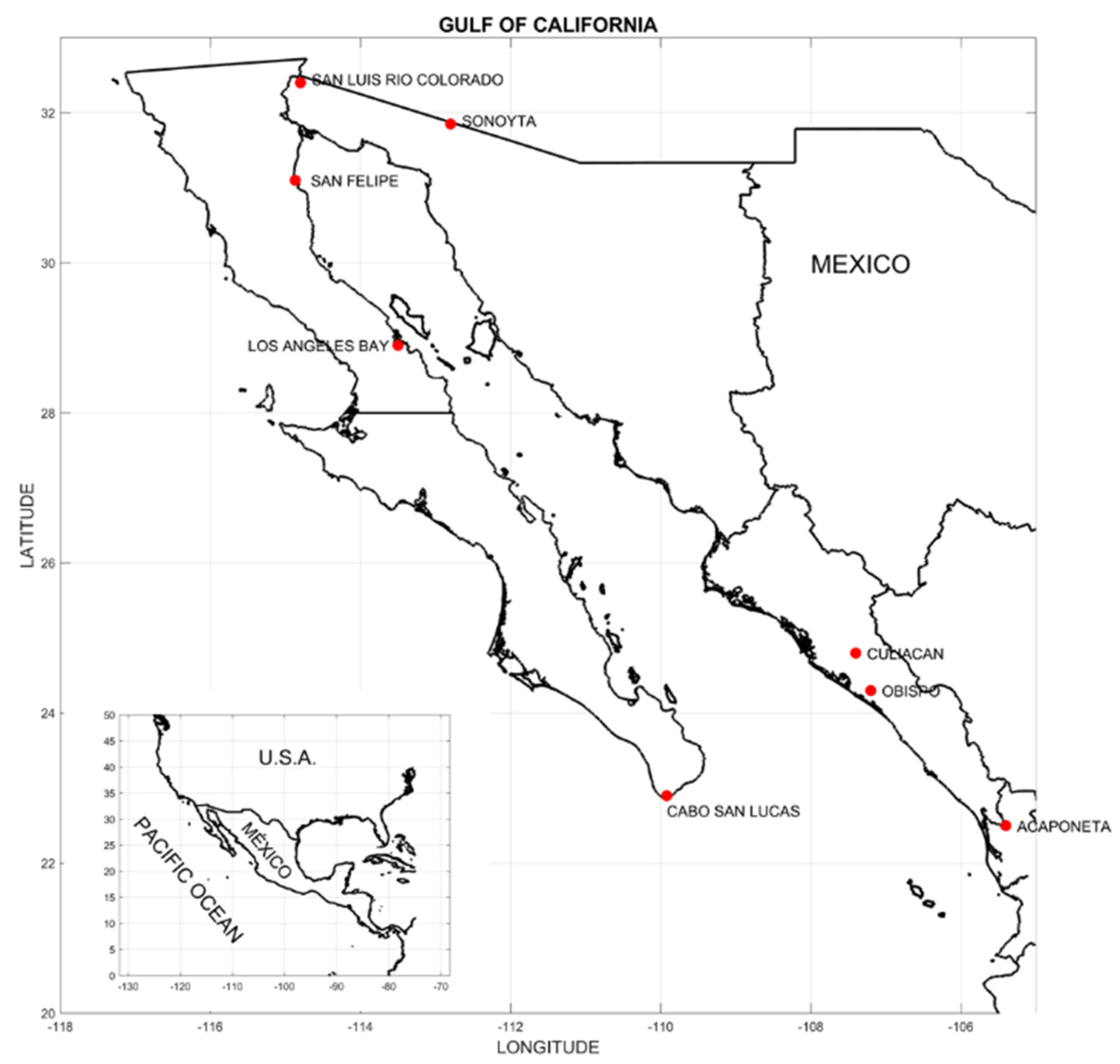
The Gulf of California

2. Data Processing and Methods
2.1. Data
2.2. Harmonic Analysis
2.3. Empirical Orthogonal Functions
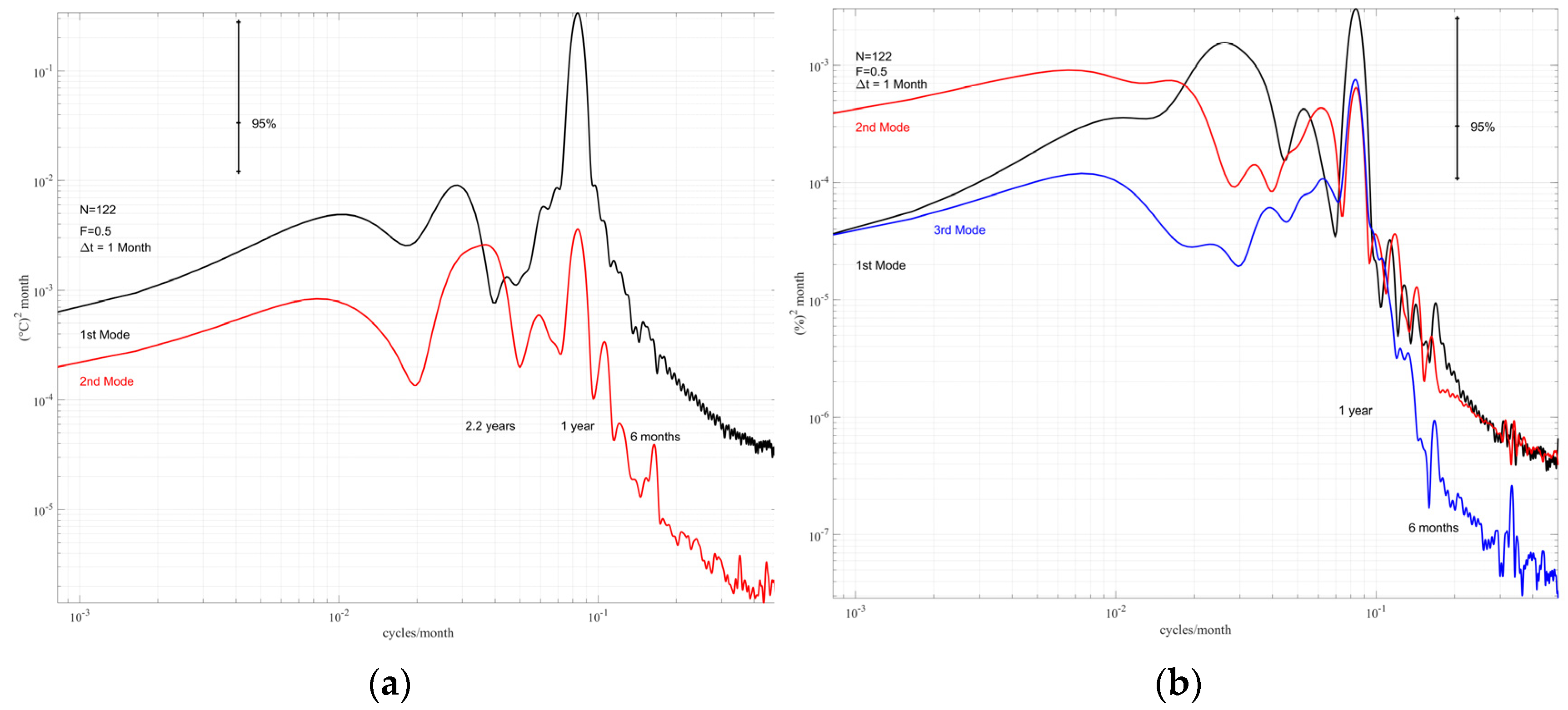
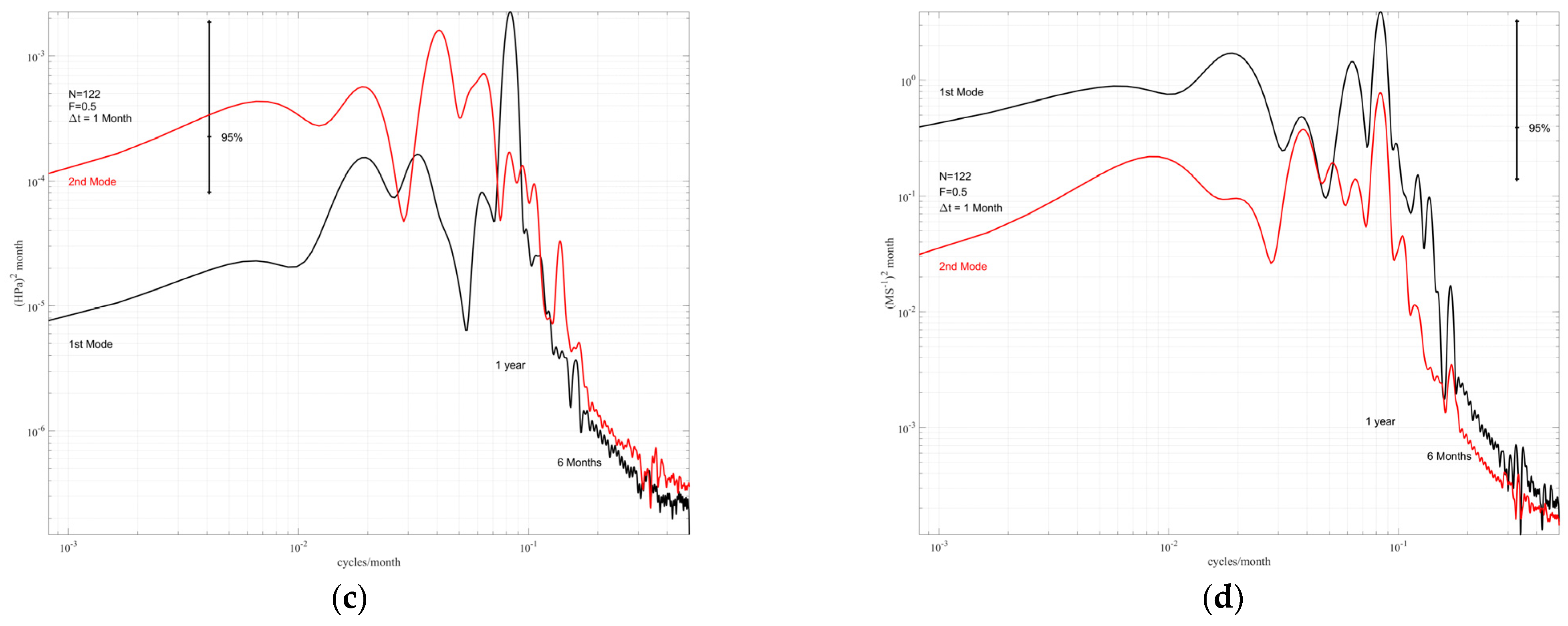
2.4. Spectral Analysis
2.5. Interpolation
2.6. Correlation Coefficient
3. Results
3.1. Harmonic Analysis
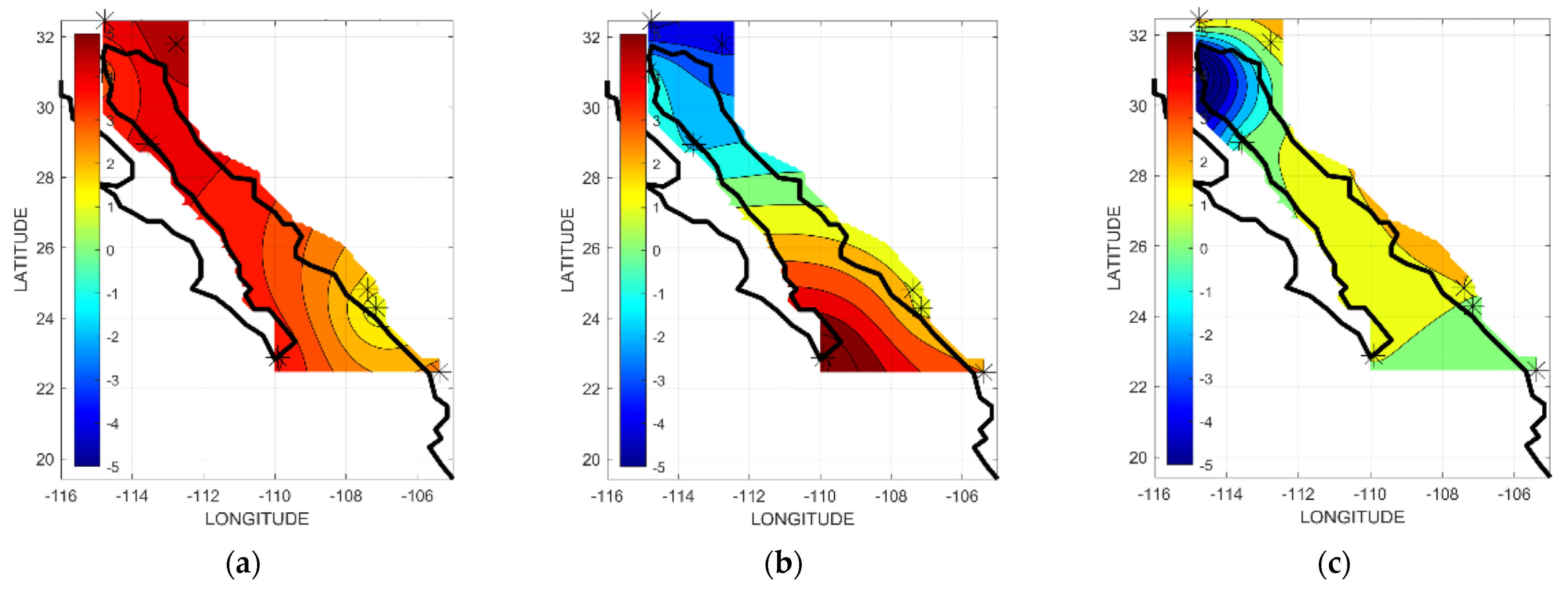
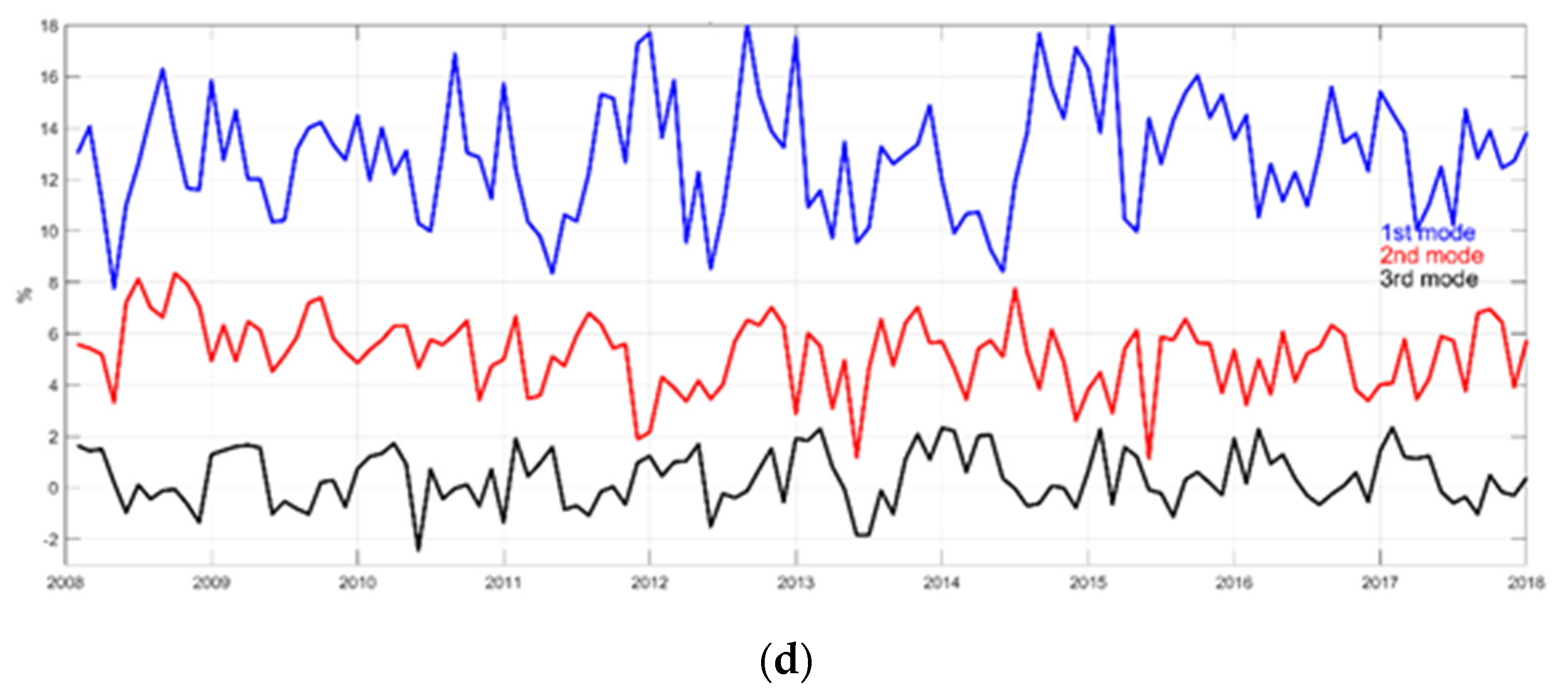
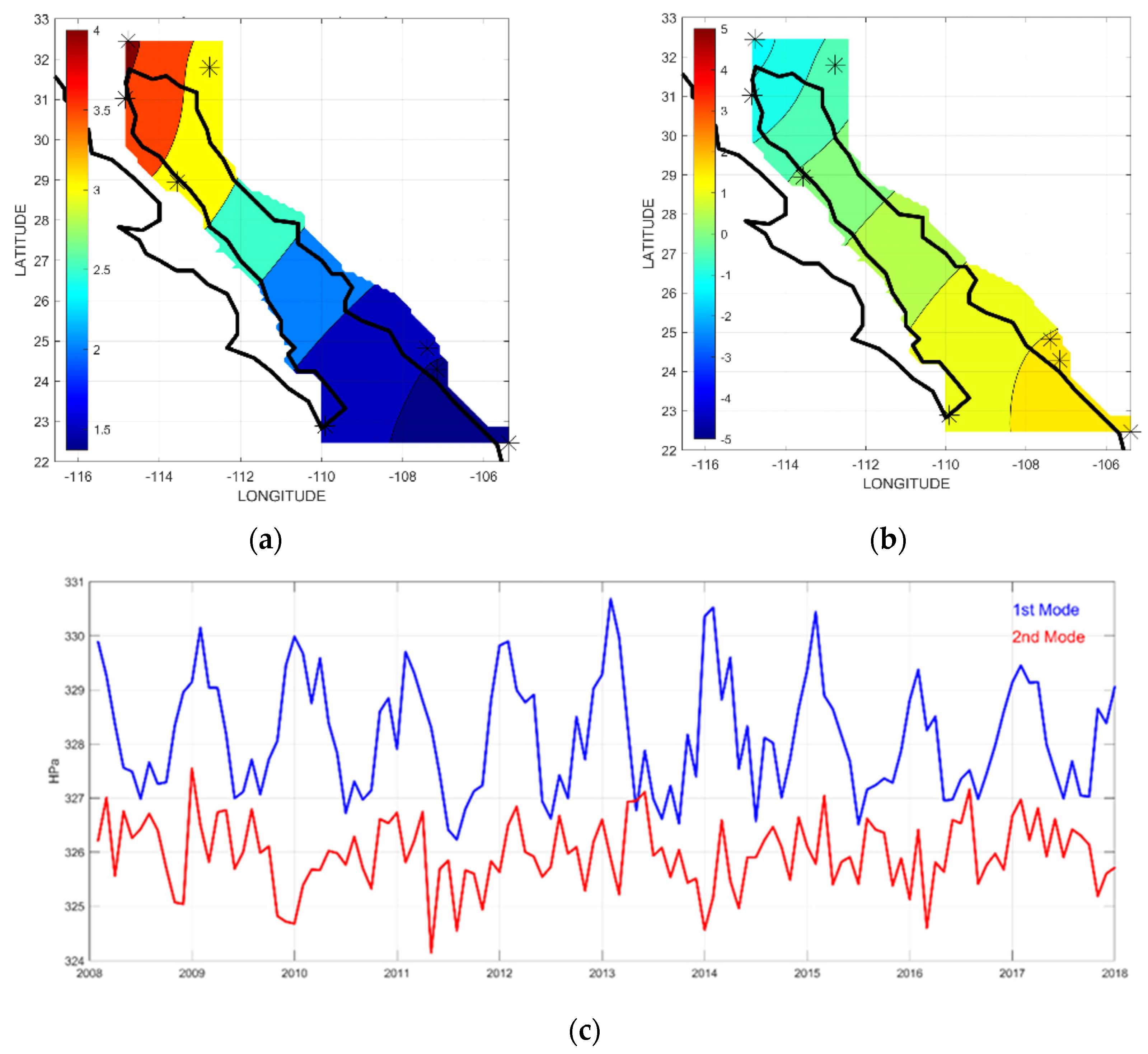
3.2. Empirical Orthogonal Functions (EOFs)
4. Discussion
4.1. Seasonal Variation
4.1.1. Air Temperature
4.1.2. Relative Humidity
4.1.3. Atmospheric Pressure
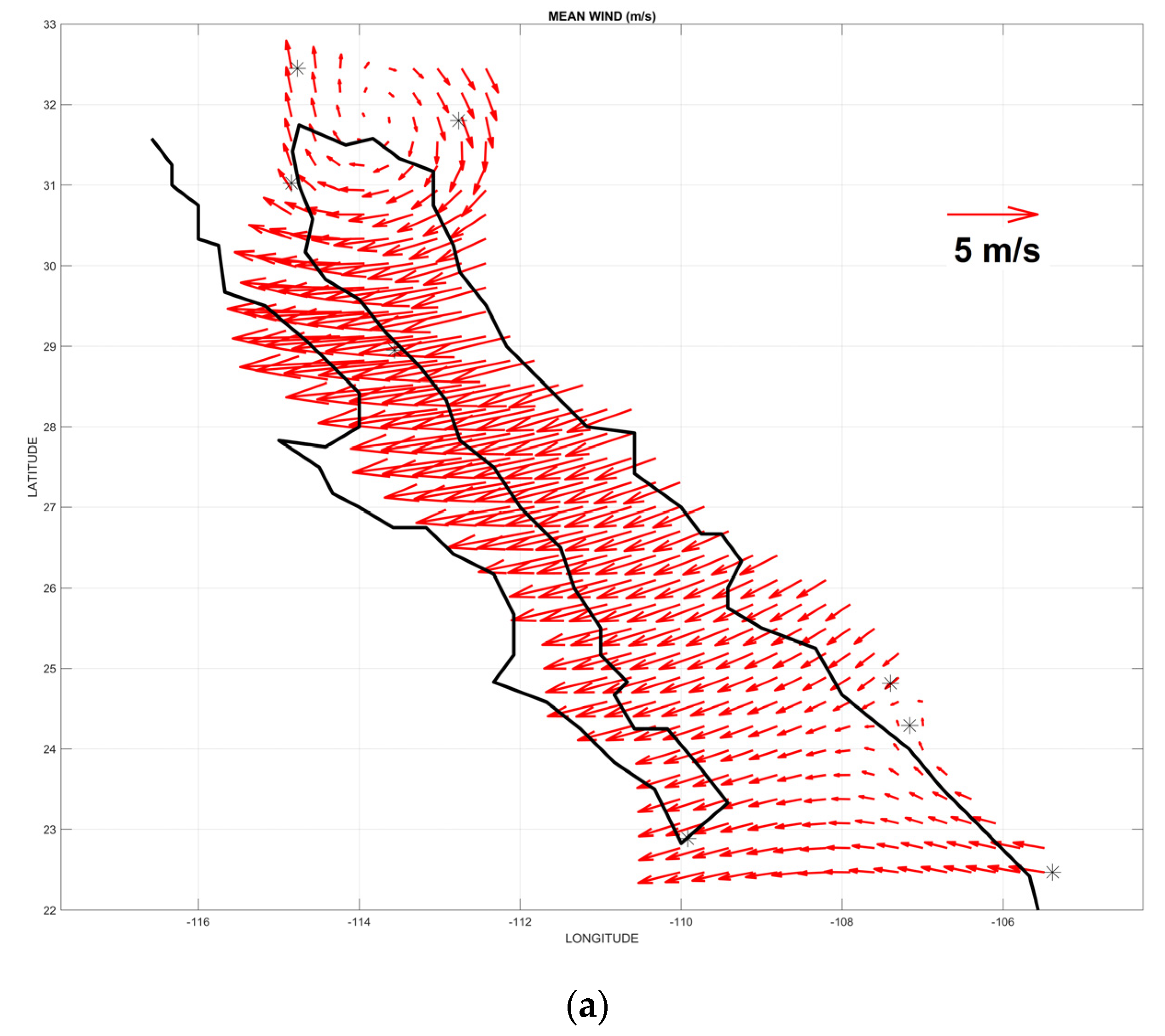
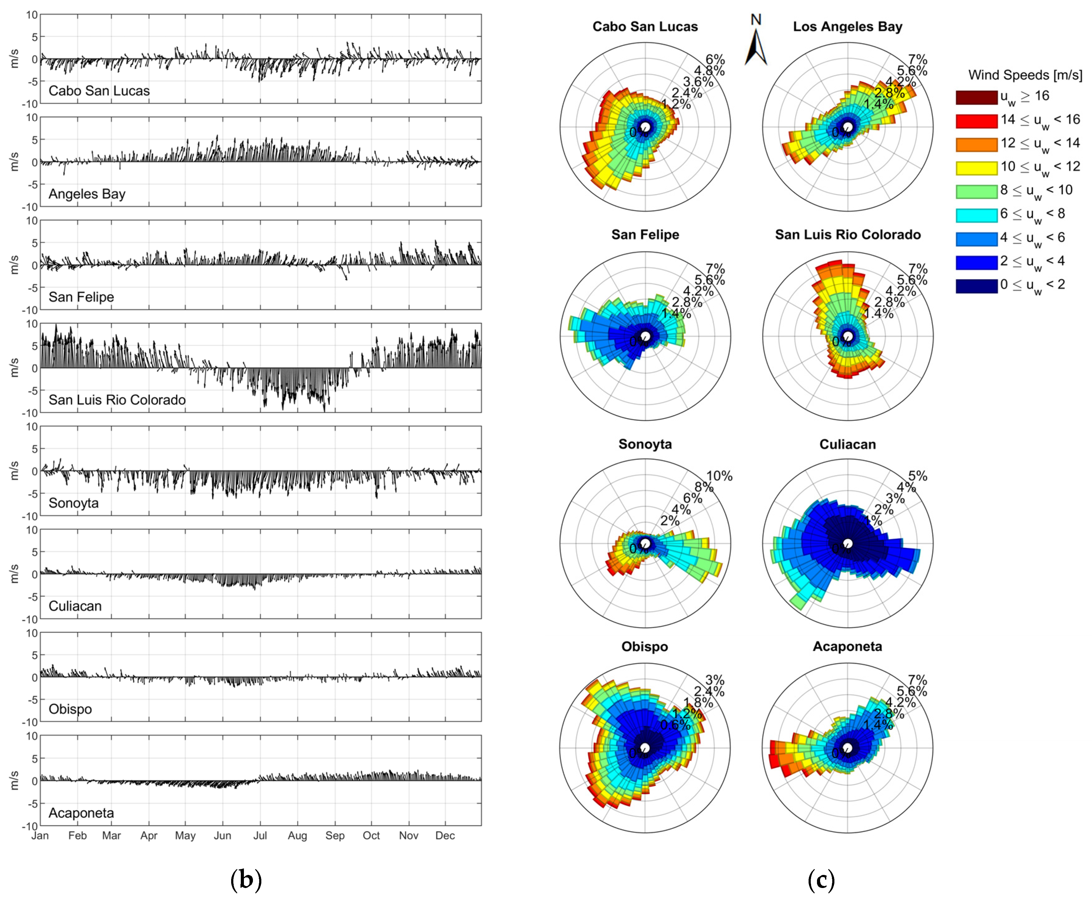
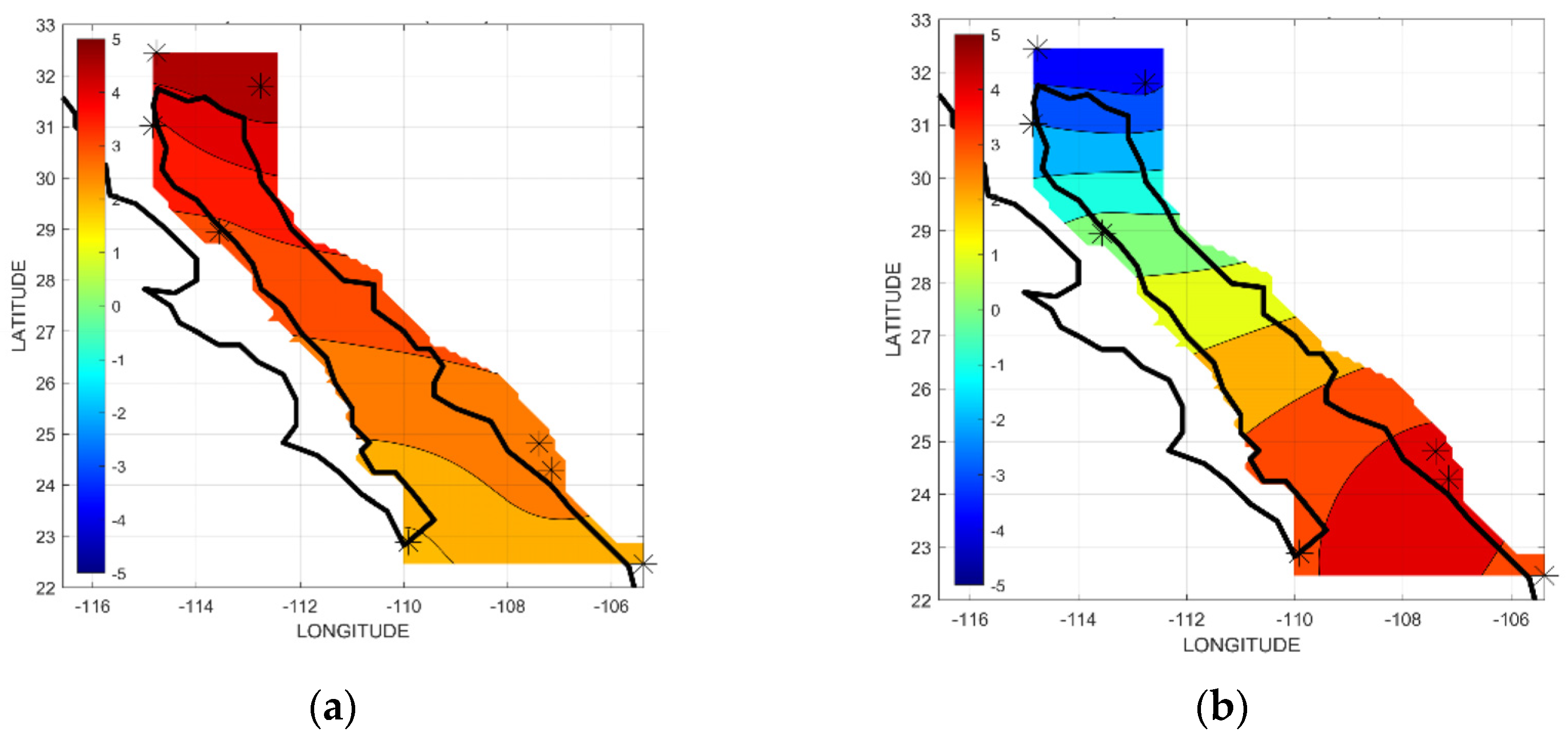
4.1.4. Wind
4.2. Seasonal Synoptic Patterns
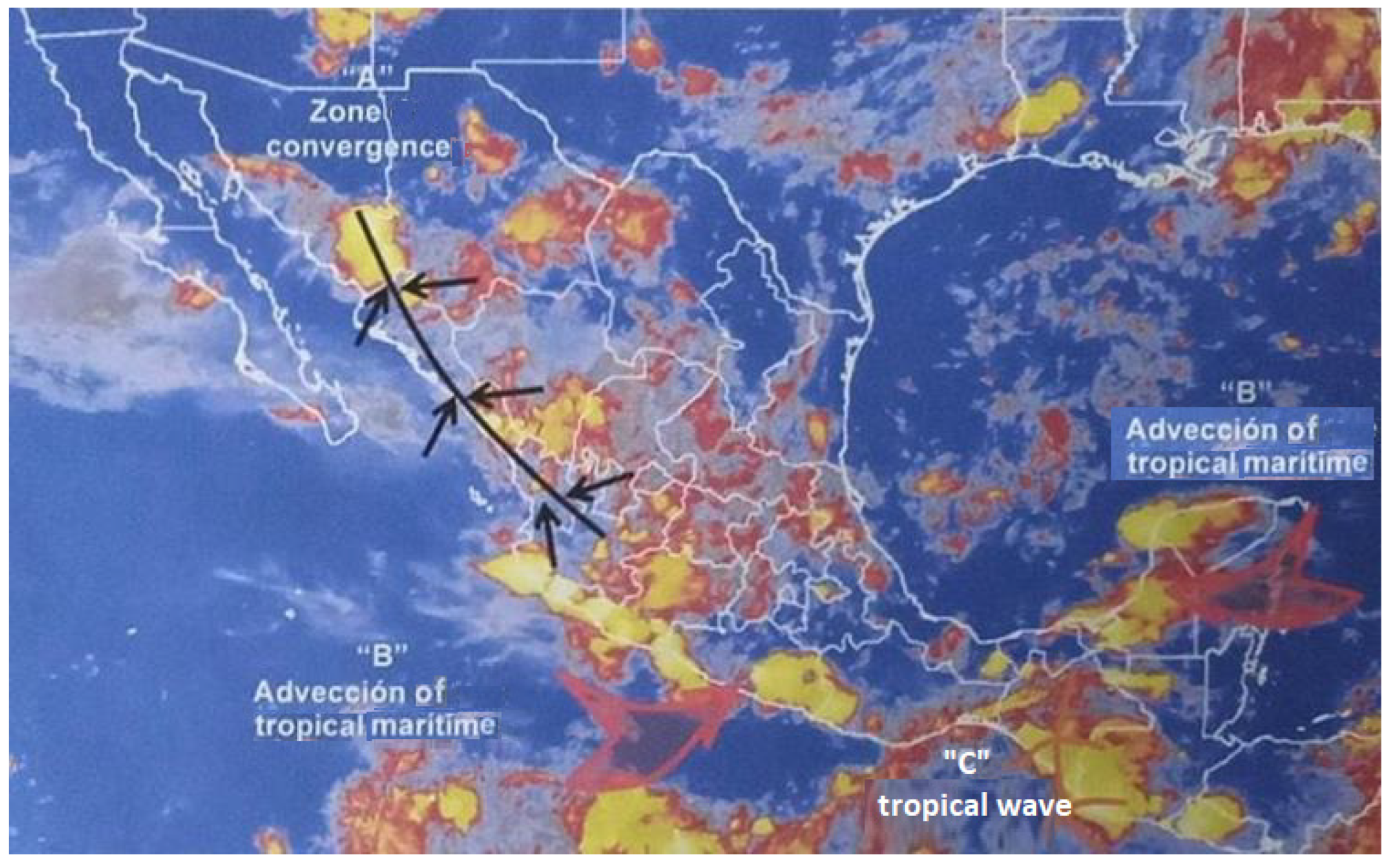
4.2.1. Summer
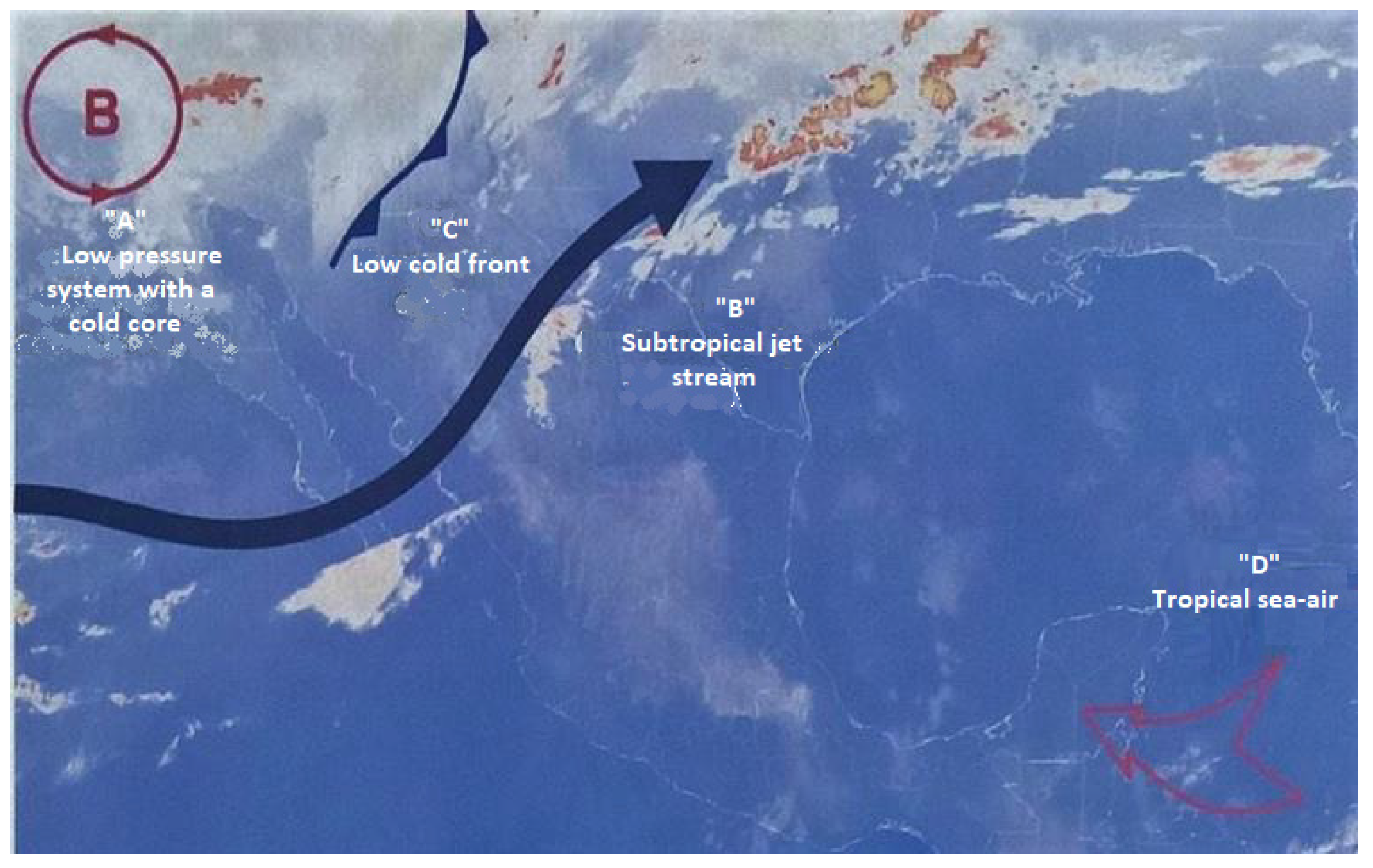
4.2.2. Winter
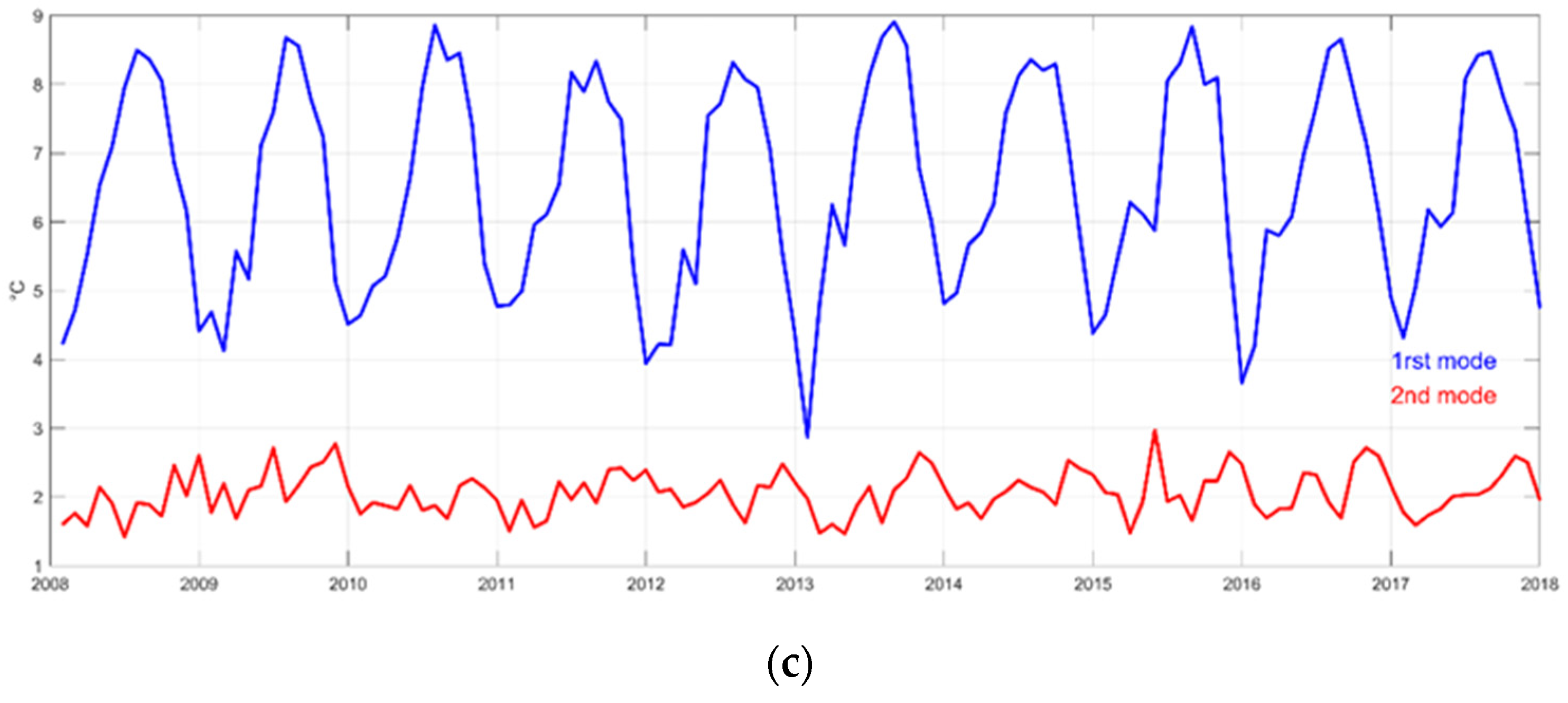
4.3. Interannual Variation
5. Conclusions
Author Contributions
Funding
Data Availability Statement
Acknowledgments
Conflicts of Interest
Appendix A

References
- Farfán, L.M.; Barrett, B.S.; Raga, G.B.; Delgado, J.J. Characteristics of mesoscale convection over northwestern Mexico, the Gulf of California, and Baja California Peninsula. Int. J. Climatol. 2021, 41, E1062–E1084. [Google Scholar] [CrossRef]
- Gochis, D.J.; Watts, C.J.; Garatuza-Payan, J.; Cesar-Rodriguez, J. Spatial and Temporal Patterns of Precipitation Intensity as Observed by the NAME Event Rain Gauge Network from 2002 to 2004. J. Clim. 2007, 20, 1734–1750. [Google Scholar] [CrossRef] [Green Version]
- Nesbitt, S.W.; Gochis, D.J.; Lang, T.J. The Diurnal Cycle of Clouds and Precipitation along the Sierra Madre Occidental Observed during NAME-2004: Implications for Warm Season Precipitation Estimation in Complex Terrain. J. Hydrometeorol. 2008, 9, 728–743. [Google Scholar] [CrossRef] [Green Version]
- Rowe, A.K.; Rutledge, S.A.; Lang, T.J.; Ciesielski, P.E.; Saleeby, S.M. Elevation-Dependent Trends in Precipitation Observed during NAME. Mon. Weather Rev. 2008, 136, 4962–4979. [Google Scholar] [CrossRef]
- Arriaga-Ramírez, S.; Cavazos, T. Regional trends of daily precipitation indices in northwest Mexico and southwest United States. J. Geophys. Res. Atmos. 2010, 115, D14111. [Google Scholar] [CrossRef]
- Brito-Castillo, L.; Díaz-Castro, S.; Salinas-Zavala, C.A.; Douglas, A.V. Reconstruction of long-term winter streamflow in the Gulf of California continental watershed. J. Hydrol. 2003, 278, 39–50. [Google Scholar] [CrossRef]
- Castillo, M.; Muñoz-Salinas, E.; Sanderson, D.C.W.; Cresswell, A. Landscape evolution of Punta Arena sand spit (SE Baja California Peninsula, NW Mexico): Implications of ENSO on landscape erosion rates. Catena 2020, 193, 104601. [Google Scholar] [CrossRef]
- Cavazos, T.; Luna-Niño, R.; Cerezo-Mota, R.; Fuentes-Franco, R.; Méndez, M.; Pineda Martínez, L.F.; Valenzuela, E. Climatic trends and regional climate models intercomparison over the CORDEX-CAM (Central America, Caribbean, and Mexico) domain. Int. J. Climatol. 2020, 40, 1396–1420. [Google Scholar] [CrossRef]
- Conde Alvarez, A.C. Cambio y Variabilidad Climáticos. Dos Estudios de Caso en México. Ph.D. Thesis, Universidad Nacional Autónoma de México, Distrito Federal, Mexico, 2003. [Google Scholar]
- Del-Toro-Guerrero, F.J.; Kretzschmar, T. Precipitation-temperature variability and drought episodes in northwest Baja California, México. J. Hydrol. Reg. Stud. 2020, 27, 100653. [Google Scholar] [CrossRef]
- Diaz, S.C.; Salinas-Zavala, C.A.; Arriaga, L. An interannual climatological aridity series for the Sierra de La Laguna, B.C.S. Mexico. Mt. Res. Dev. 1994, 14, 137–146. [Google Scholar] [CrossRef]
- Dominguez, C.; Jaramillo, A.; Cuéllar, P. Are the socioeconomic impacts associated with tropical cyclones in Mexico exacerbated by local vulnerability and ENSO conditions? Int. J. Climatol. 2021, 41, E3307–E3324. [Google Scholar] [CrossRef]
- Morales-Acuña, E.; Torres, C.; Delgadillo-Hinojosa, F.; Linero-Cueto, J.; Santamaría-Del-Ángel, E.; Castro, R. The Baja California Peninsula, a Significant Source of Dust in Northwest Mexico. Atmosphere 2019, 10, 582. [Google Scholar] [CrossRef] [Green Version]
- Pavia, E.G.; Graef, F.; Reyes, J. PDO–ENSO Effects in the Climate of Mexico. J. Clim. 2006, 19, 6433–6438. [Google Scholar] [CrossRef]
- Brito-Castillo, L.; Douglas, A.V.; Leyva-Contreras, A.; Lluch-Belda, D. The effect of large-scale circulation on precipitation and streamflow in the Gulf of California continental watershed. Int. J. Climatol. 2003, 23, 751–768. [Google Scholar] [CrossRef]
- Higgins, R.W.; Silva, V.B.S.; Shi, W.; Larson, J. Relationships between climate variability and fluctuations in daily precipitation over the United States. J. Clim. 2007, 20, 3561–3579. [Google Scholar] [CrossRef]
- Mantua, N.J.; Hare, S.R. The Pacific Decadal Oscillation. J. Oceanogr. 2002, 58, 35–44. [Google Scholar] [CrossRef]
- Torres, V.M.; Thorncroft, C.D. Interdecadal Variability of Easterly Waves Over the Tropical Northeastern Pacific. Geophys. Res. Lett. 2022, 49, e2022GL099090. [Google Scholar] [CrossRef]
- Wright, K.T.; Johnson, K.R.; Bhattacharya, T.; Marks, G.S.; McGee, D.; Elsbury, D.; Peings, Y.; Lacaille-Muzquiz, J.-L.; Lum, G.; Beramendi-Orosco, L.; et al. Precipitation in Northeast Mexico Primarily Controlled by the Relative Warming of Atlantic SSTs. Geophys. Res. Lett. 2022, 49, e2022GL098186. [Google Scholar] [CrossRef]
- Brito-Castillo, L.; Alcocer-Vázquez, M.D.; Félix-Domínguez, J.E. Características de los vientos superficiales en Sonora: Información relevante para el aprovechamiento del recurso y prevención de desastres. Quehacer Científico En Chiapas 2019, 14, 33–45. [Google Scholar]
- Bordoni, S.; Ciesielski, P.E.; Johnson, R.H.; McNoldy, B.D.; Stevens, B. The low-level circulation of the North American Monsoon as revealed by QuikSCAT. Geophys. Res. Lett. 2004, 31, L10109. [Google Scholar] [CrossRef] [Green Version]
- Bordoni, S.; Stevens, B. Principal Component Analysis of the Summertime Winds over the Gulf of California: A Gulf Surge Index. Mon. Weather Rev. 2006, 134, 3395–3414. [Google Scholar] [CrossRef] [Green Version]
- Douglas, M.W. The Summertime Low-Level Jet over the Gulf of California. Mon. Weather Rev. 1995, 123, 2334–2347. [Google Scholar] [CrossRef]
- Stensrud, D.J.; Gall, R.L.; Nordquist, M.K. Surges over the Gulf of California during the Mexican Monsoon. Mon. Weather Rev. 1997, 125, 417–437. [Google Scholar] [CrossRef]
- Douglas, M.W.; Valdez-Manzanilla, A.; Garcia Cueto, R. Diurnal Variation and Horizontal Extent of the Low-Level Jet over the Northern Gulf of California. Mon. Weather Rev. 1998, 126, 2017–2025. [Google Scholar] [CrossRef]
- Ciesielski, P.E.; Johnson, R.H. Diurnal Cycle of Surface Flows during 2004 NAME and Comparison to Model Reanalysis. J. Clim. 2008, 21, 3890–3913. [Google Scholar] [CrossRef]
- IPCC. Climate Change 2021: The Physical Science Basis; Masson-Delmotte, V., Zhai, P., Pirani, A., Connors, S.L., Péan, C., Berger, S., Caud, N., Chen, Y., Goldfarb, L., Gomis, M., Eds.; Cambridge University Press: Cambridge, UK; New York, NY, USA, 2021; Volume 2, p. 2391. [Google Scholar]
- Ripple, W.J.; Wolf, C.; Gregg, J.W.; Levin, K.; Rockström, J.; Newsome, T.M.; Betts, M.G.; Huq, S.; Law, B.E.; Kemp, L.; et al. World Scientists’ Warning of a Climate Emergency 2022. BioScience 2022, 72, 1149–1155. [Google Scholar] [CrossRef]
- Wang, S.; Toumi, R. Recent tropical cyclone changes inferred from ocean surface temperature cold wakes. Sci. Rep. 2021, 11, 22269. [Google Scholar] [CrossRef]
- Magaña Rueda, V.O. Los Impactos de el Niño en México; Universidad Nacional Autónoma de México: Mexico City, Mexico, 2001. [Google Scholar]
- García, E. Modificaciones al Sistema de Clasificación Climática de Koppen; (Para Adaptarlo a las Condiciones de la República Mexicana); Universidad Nacional Autónoma de México: Mexico City, Mexico, 1987. [Google Scholar]
- Douglas, M.W.; Maddox, R.A.; Howard, K.; Reyes, S. The Mexican Monsoon. J. Clim. 1993, 6, 1665–1677. [Google Scholar] [CrossRef]
- Barlow, M.; Nigam, S.; Berbery, E.H. Evolution of the North American Monsoon System. J. Clim. 1998, 11, 2238–2257. [Google Scholar] [CrossRef]
- Gochis, D.J.; Brito-Castillo, L.; Shuttleworth, W.J. Hydroclimatology of the North American Monsoon region in northwest Mexico. J. Hydrol. 2006, 316, 53–70. [Google Scholar] [CrossRef]
- Verduzco, V.S.; Garatuza-Payán, J.; Yépez, E.A.; Watts, C.J.; Rodríguez, J.C.; Robles-Morua, A.; Vivoni, E.R. Variations of net ecosystem production due to seasonal precipitation differences in a tropical dry forest of northwest Mexico. J. Geophys. Res. Biogeosci. 2015, 120, 2081–2094. [Google Scholar] [CrossRef]
- Brito-Castillo, L.; Farfán, L.M.; Antemate-Velasco, G.J. Effect of the Trans-Volcanic Axis on meridional propagation of summer precipitation in western Mexico. Int. J. Climatol. 2022, 42, 9304–9318. [Google Scholar] [CrossRef]
- Wang, C.; Fiedler, P.C. ENSO variability and the eastern tropical Pacific: A review. Prog. Oceanogr. 2006, 69, 239–266. [Google Scholar] [CrossRef]
- Bernal, G.; Ripa, P.; Herguera, J.C. Oceanographic and climatic variability in the lower Gulf of California: Links with the tropics and North Pacific. Cienc. Mar. 2001, 27, 595–617. [Google Scholar] [CrossRef] [Green Version]
- Dunkerley, D. The Ecohydrology of Desert Environments: What Makes it Distinctive? In Encyclopedia of the World’s Biomes; Goldstein, M.I., DellaSala, D.A., Eds.; Elsevier: Oxford, UK, 2020; pp. 23–35. [Google Scholar]
- Schmidt, R.H. The arid zones of Mexico: Climatic extremes and conceptualization of the Sonoran Desert. J. Arid Environ. 1989, 16, 241–256. [Google Scholar] [CrossRef]
- Reyes, S.; Douglas, M.W.; Maddox, R.A. El monzón del suroeste de Norteamérica (TRAVASON/SWAMP). Atmósfera 1994, 7, 117–137. [Google Scholar]
- Ripa, P. Least squares data fitting. Cienc. Mar. 2002, 28, 79–105. [Google Scholar] [CrossRef] [Green Version]
- Cepeda-Morales, J.; Gaxiola-Castro, G.; Beier, E.; Godínez, V.M. The mechanisms involved in defining the northern boundary of the shallow oxygen minimum zone in the eastern tropical Pacific Ocean off Mexico. Deep Sea Res. Part I Oceanogr. Res. Pap. 2013, 76, 1–12. [Google Scholar] [CrossRef]
- Olascoaga, M.J.; Beron-Vera, F.J.; Miron, P.; Triñanes, J.; Putman, N.F.; Lumpkin, R.; Goni, G.J. Observation and quantification of inertial effects on the drift of floating objects at the ocean surface. Phys. Fluids 2020, 32, 026601. [Google Scholar] [CrossRef]
- Oliver, M.A.; Webster, R. Kriging: A method of interpolation for geographical information systems. Int. J. Geogr. Inf. Syst. 1990, 4, 313–332. [Google Scholar] [CrossRef]
- Amador, J.A.; Alfaro, E.J.; Lizano, O.G.; Magaña, V.O. Atmospheric forcing of the eastern tropical Pacific: A review. Prog. Oceanogr. 2006, 69, 101–142. [Google Scholar] [CrossRef]
- Neiburger, M.; Edinger, J.G.; Bonner, W.D. Understanding Our Atmospheric Environment; W.H. Freeman: New York, NY, USA, 1973. [Google Scholar]
- Wu, M.-L.C.; Schubert, S.D.; Suarez, M.J.; Huang, N.E. An Analysis of Moisture Fluxes into the Gulf of California. J. Clim. 2009, 22, 2216–2239. [Google Scholar] [CrossRef]
- Hales, J.E. Surges of Maritime Tropical Air Northward Over the Gulf of California. Mon. Weather Rev. 1972, 100, 298–306. [Google Scholar] [CrossRef]
- Brenner, I.S. A Surge of Maritime Tropical Air—Gulf of California to the Southwestern United States. Mon. Weather Rev. 1974, 102, 375–389. [Google Scholar] [CrossRef]
- Amador, J.A.; Arce-Fernández, D. WWLLN Hot and Cold-Spots of Lightning Activity and Their Relation to Climate in an Extended Central America Region 2012–2020. Atmosphere 2022, 13, 76. [Google Scholar] [CrossRef]
- Willeit, M.; Ganopolski, A.; Robinson, A.; Edwards, N.R. The Earth system model CLIMBER-X v1.0—Part 1: Climate model description and validation. Geosci. Model Dev. 2022, 15, 5905–5948. [Google Scholar] [CrossRef]
- Lin, J.; Qian, T.; Bechtold, P.; Grell, G.; Zhang, G.J.; Zhu, P.; Freitas, S.R.; Barnes, H.; Han, J. Atmospheric Convection. Atmosphere-Ocean 2022, 60, 422–476. [Google Scholar] [CrossRef]
- Ramos-Pérez, O.; Adams, D.K.; Ochoa-Moya, C.A.; Quintanar, A.I. A Climatology of Mesoscale Convective Systems in Northwest Mexico during the North American Monsoon. Atmosphere 2022, 13, 665. [Google Scholar] [CrossRef]
- Clapp, C.E.; Smith, J.B.; Bedka, K.M.; Anderson, J.G. Identifying Outflow Regions of North American Monsoon Anticyclone-Mediated Meridional Transport of Convectively Influenced Air Masses in the Lower Stratosphere. J. Geophys. Res. Atmos. 2021, 126, e2021JD034644. [Google Scholar] [CrossRef]
- Colorado-Ruiz, G.; Cavazos, T. Trends of daily extreme and non-extreme rainfall indices and intercomparison with different gridded data sets over Mexico and the southern United States. Int. J. Climatol. 2021, 41, 5406–5430. [Google Scholar] [CrossRef]
- Cortés-Ramos, J.; Farfán, L.M.; Brito-Castillo, L. Extreme freezing in the Sonoran Desert, Mexico: Intense and short-duration events. Int. J. Climatol. 2021, 41, 4339–4358. [Google Scholar] [CrossRef]
- Jáuregui, E.; Cruz Navarro, F. Algunos aspectos del clima de Sonora y Baja California: Equipatas y surgencias de humedad. Investig. Geográficas 1980, 143–180. [Google Scholar] [CrossRef]
- Gaxiola-Morales, M.G.; Brito-Castillo, L. Análisis de los factores de radiación-evapotranspiración en el Desierto Sonorense. Biotecnia 2019, 21, 137–144. [Google Scholar] [CrossRef]
- NOAA. Multivariate ENSO Index Version 2 (MEI.v2). Available online: https://psl.noaa.gov/enso/mei/ (accessed on 23 February 2022).
- NOAA. Southern Oscillation Index (SOI). Available online: https://www.ncdc.noaa.gov/teleconnections/enso/indicators/soi/ (accessed on 23 February 2022).
- Quiroz, M. Anexo del Informe Técnico: Elaboración de un Boletín con Información Hidroclimática de los Mares de México; INAPESCA: Ciudad de México, Mexico, 2011; p. 27. [Google Scholar]
- Zolotokrylin, A.N.; Titkova, T.B.; Brito-Castillo, L. Wet and dry patterns associated with ENSO events in the Sonoran Desert from, 2000–2015. J. Arid Environ. 2016, 134, 21–32. [Google Scholar] [CrossRef]
- Vega-Camarena, J.P.; Brito-Castillo, L.; Pineda-Martínez, L.F.; Farfán, L.M. ENSO Impact on Summer Precipitation and Moisture Fluxes over the Mexican Altiplano. J. Mar. Sci. Eng. 2023, 11, 1083. [Google Scholar] [CrossRef]
- Vega-Camarena, J.P.; Brito-Castillo, L.; Farfán, L.M.; Gochis, D.J.; Pineda-Martínez, L.F.; Díaz, S.C. Ocean–atmosphere conditions related to severe and persistent droughts in the Mexican Altiplano. Int. J. Climatol. 2018, 38, 853–866. [Google Scholar] [CrossRef]
- Rasmusson, E.M.; Wallace, J.M. Meteorological Aspects of the El Niño/Southern Oscillation. Science 1983, 222, 1195–1202. [Google Scholar] [CrossRef]
- Castro, L.C.; McKee, T.B.; Pielke, R.A. The Relationship of the North American Monsoon to Tropical and North Pacific Sea Surface Temperatures as Revealed by Observational Analyses. J. Clim. 2001, 14, 4449–4473. [Google Scholar] [CrossRef]
- Reyes, S.; Mejía-Trejo, A. Tropical perturbations in the Eastern Pacific and the Precipitation field over North-Western Mexico in relation to the enso phenomenon. Int. J. Climatol. 1991, 11, 515–528. [Google Scholar] [CrossRef]
- Seager, R.; Kushnir, Y.; Herweijer, C.; Naik, N.; Velez, J. Modeling of Tropical Forcing of Persistent Droughts and Pluvials over Western North America: 1856–2000. J. Clim. 2005, 18, 4065–4088. [Google Scholar] [CrossRef]
- Martinez-Sanchez, J.N.; Cavazos, T. Eastern Tropical Pacific hurricane variability and landfalls on Mexican coasts. Clim. Res. 2014, 58, 221–234. [Google Scholar] [CrossRef]
- Johnson, B.O.; Delworth, T.L. The Role of the Gulf of California in the North American Monsoon. J. Clim. 2023, 36, 1541–1559. [Google Scholar] [CrossRef]


| Number-Station | Label | Altitude (m) | Latitude (N)/ Longitude (W) |
|---|---|---|---|
| CLS | 35 | 22°54′00.52″/ |
| 109°55′00.12″ | |||
| BLA | 4 | 28°57′07.68″/ 113°33′44.83″ |
| SFL | 15 | 31°01′34.50″/ 114°50′29.37″ |
| SRC | 42 | 32°27′08.89″/ 114°46′17.88″ |
| SNY | 389 | 31°56′48.20″/ 112°45′55.77″ |
| CLC | 60 | 24°48′54.73″/ 107°23′51.94″ |
| OBP | 37 | 24°17′32.84″/ 107°09′31.93″ |
| ACP | 24 | 22°28′04.59″/ 105°23′02.72″ |
| Variable | CSL | BLA | SFL | SRC | SNY | CLC | OBP | ACP | |
|---|---|---|---|---|---|---|---|---|---|
| TEMP. (°C) | 24.5 | 24.3 | 24.5 | 24.3 | 23.0 | 25.0 | 24.1 | 25.3 | |
| A. P. (HPa) | 1013.4 | 1010.4 | 1009.3 | 1009.9 | 1009.2 | 1009.8 | 1010.1 | 1009.4 | |
| Mean | R. H. (%) | 58.5 | 42.4 | 40.5 | 40.0 | 37.7 | 66.8 | 75.5 | 71.4 |
| U (m/s) | −2.19 | −7.45 | −0.52 | −0.27 | 0.63 | −0.80 | 0.08 | −2.02 | |
| V (m/s) | −0.69 | −0.60 | 1.17 | 1.53 | −1.65 | −0.68 | 0.50 | 0.28 | |
| TEMP. (°C) | 3.69 7.7 | 6.86 7.6 | 7.66 7.4 | 9.69 7.1 | 9.94 7.0 | 5.93 7.5 | 6.32 7.8 | 4.47 7.4 | |
| A. P. (HPa) | 2.06 0.9 | 4.39 1.1 | 5.30 0.8 | 5.56 0.9 | 4.02 0.8 | 2.12 1.2 | 1.87 1.3 | 1.79 1.4 | |
| / | R. H. (%) | 10.57 9.3 | 5.78 10.0 | 10.87 8.5 | 7.67 11.7 | 10.75 10.8 | 3.21 10.2 | 2.0 9.5 | 8.57 9.5 |
| U (m/s) | 1.10 6.0 | 0.95 0.3 | 2.00 6.7 | 1.06 10.0 | 2.66 0.4 | 0.25 11.7 | 0.40 0.0 | 2.03 10.4 | |
| V (m/s) | 0.56 0.0 | 3.64 1.3 | 0.63 1.3 | 5.43 1.0 | 2.56 0.3 | 1.54 11.7 | 0.29 0.0 | 1.24 10.4 | |
| TEMP. (°C) | 0.65 3.5 | 1.29 2.5 | 1.85 2.6 | 2.29 2.4 | 2.19 2.5 | 0.88 3.8 | 0.82 3.9 | 0.82 4.4 | |
| A. P. (HPa) | 0.60 1.2 | 0.73 1.0 | 0.91 0.7 | 0.55 1.0 | 1.09 1.2 | 0.91 1.0 | 0.65 1.2 | 0.67 1.3 | |
| / | R. H. (%) | 4.82 1.6 | 6.65 1.9 | 3.80 0.3 | 4.44 1.4 | 2.74 1.0 | 5.89 2.0 | 3.94 2.3 | 4.61 1.9 |
| U (m/s) | 0.82 4.4 | 4.15 2.2 | 0.62 1.9 | 0.59 0.6 | 0.22 4.1 | 0.30 2.9 | 0.22 3.1 | 0.50 1.5 | |
| V (m/s) | 1.04 4.9 | 2.03 1.9 | 0.53 5.2 | 2.09 4.1 | 0.78 2.1 | 0.10 1.3 | 0.03 5.4 | 0.28 3.1 | |
| TEMP. (°C) | 0.63 2.3 | 0.85 2.4 | 0.56 2.6 | 1.08 2.4 | 0.95 2.2 | 0.95 2.1 | 1.0 2.2 | 1.02 1.8 | |
| A. P. (HPa) | 0.33 3.4 | 0.42 0.0 | 0.21 3.9 | 0.36 3.5 | 0.27 0.1 | 0.22 3.9 | 0.25 3.9 | 0.36 3.6 | |
| / | R. H. (%) | 2.65 0.3 | 1.69 0.3 | 1.61 3.4 | 2.52 3.8 | 4.84 3.8 | 0.48 0.5 | 0.63 3.7 | 1.27 0.5 |
| U (m/s) | 0.49 0.7 | 2.15 3.4 | 0.27 3.5 | 0.27 1.9 | 0.72 2.2 | 0.06 3.1 | 0.12 1.9 | 0.59 3.7 | |
| V (m/s) | 0.20 1.8 | 1.19 0.2 | 0.01 2.0 | 1.42 1.1 | 1.11 2.3 | 0.38 0.1 | 0.19 0.3 | 0.28 3.4 | |
| TEMP. (°C) | 0.37 2.0 | 0.40 0.2 | 0.19 0.5 | 0.27 2.9 | 0.38 0.0 | 0.18 2.3 | 0.35 2.6 | 0.26 2.4 | |
| A. P. (HPa) | 0.24 1.0 | 0.62 1.0 | 0.60 1.1 | 0.58 1.2 | 0.60 1.0 | 0.19 1.2 | 0.14 1.1 | 0.10 1.7 | |
| / | R. H. (%) | 1.71 0.3 | 3.90 2.1 | 5.71 2.1 | 2.14 2.1 | 2.88 2.2 | 1.25 2.9 | 1.19 2.4 | 2.98 0.7 |
| U (m/s) | 0.77 2.2 | 1.21 2.3 | 0.32 2.8 | 0.44 2.2 | 0.67 2.7 | 0.24 2.6 | 0.07 0.4 | 0.08 1.3 | |
| V (m/s) | 0.84 2.8 | 1.50 1.0 | 0.34 0.6 | 0.85 0.4 | 1.08 1.1 | 0.32 1.5 | 0.09 2.5 | 0.18 1.3 | |
| TEMP. | 62.2 | 87.7 | 85.8 | 88.1 | 90.5 | 92.3 | 93.9 | 92.4 | |
| A. P. | 55.2 | 75.5 | 75.9 | 77.3 | 70.8 | 64.5 | 53.3 | 56.2 | |
| EV (%) | R. H. | 35.8 | 30.2 | 58.1 | 31.2 | 43.0 | 40.7 | 23.8 | 54.3 |
| U | 47.5 | 26.7 | 53.3 | 28.8 | 60.7 | 20.3 | 93.7 | 48.0 | |
| V | 53.6 | 29.8 | 17.8 | 51.3 | 56.1 | 68.4 | 83.7 | 25.3 |
| Years | SOI | MEI | ONI | |
|---|---|---|---|---|
| June 2008 | June 2009 | −0.47 | 0.46 | 0.36 |
| February 2008 | June 2009 | −0.49 | 0.49 | 0.39 |
| March 2008 | June 2009 | −0.51 | 0.51 | 0.41 |
| April 2008 | June 2009 | −0.52 | 0.53 | 0.43 |
| May 2008 | June 2009 | −0.52 | 0.54 | 0.44 |
| June 2008 | June 2009 | −0.52 | 0.54 | 0.44 |
| July 2008 | June 2009 | −0.51 | 0.53 | 0.43 |
Disclaimer/Publisher’s Note: The statements, opinions and data contained in all publications are solely those of the individual author(s) and contributor(s) and not of MDPI and/or the editor(s). MDPI and/or the editor(s) disclaim responsibility for any injury to people or property resulting from any ideas, methods, instructions or products referred to in the content. |
© 2023 by the authors. Licensee MDPI, Basel, Switzerland. This article is an open access article distributed under the terms and conditions of the Creative Commons Attribution (CC BY) license (https://creativecommons.org/licenses/by/4.0/).
Share and Cite
Palacios-Hernández, E.; Montes-Aréchiga, J.M.; Brito-Castillo, L.; Carrillo, L.; Julián-Caballero, S.; Avalos-Cueva, D. Interannual Variability in the Coastal Zones of the Gulf of California. Climate 2023, 11, 132. https://doi.org/10.3390/cli11060132
Palacios-Hernández E, Montes-Aréchiga JM, Brito-Castillo L, Carrillo L, Julián-Caballero S, Avalos-Cueva D. Interannual Variability in the Coastal Zones of the Gulf of California. Climate. 2023; 11(6):132. https://doi.org/10.3390/cli11060132
Chicago/Turabian StylePalacios-Hernández, Emilio, Jorge Manuel Montes-Aréchiga, Luis Brito-Castillo, Laura Carrillo, Sergio Julián-Caballero, and David Avalos-Cueva. 2023. "Interannual Variability in the Coastal Zones of the Gulf of California" Climate 11, no. 6: 132. https://doi.org/10.3390/cli11060132