
Characterizing Northeast Africa Drought and Its Drivers

1
Geography Department, University of Zululand, KwaDlangezwa 3886, South Africa
2
Physics Department, University of Puerto Rico Mayagüez, Mayaguez, PR 00681, USA
Climate 2023, 11(6), 130; https://doi.org/10.3390/cli11060130
Submission received: 20 May 2023
/
Revised: 5 June 2023
/
Accepted: 8 June 2023
/
Published: 10 June 2023
(This article belongs to the Special Issue Climate System Modelling and Observations)
Abstract
:This study explores the drivers of drought over northeast (NE) Africa as represented by monthly ERA5 potential evaporation during 1970–2022. The comparisons with surface heat flux and A-pan measurements suggest that potential evaporation quantifies moisture deficits that lead to drought. A principal component (PC) analysis of potential evaporation has the following leading modes: PC-1 in the Nile Basin and PC-2 in the Rift Valley. Time scores were filtered and regressed onto fields of SST, netOLR, and 500 hPa zonal wind to find teleconnections, and drought composites were analyzed for anomalous structure. The results identify that cold-phase Indian Ocean Dipole (IOD) couples with the overlying zonal Walker circulation. Deep easterly winds subside at −0.1 m/s over the west Indian Ocean and NE Africa, causing desiccation that spreads westward from the Rift Valley via diurnal heat fluxes. Insights are gained on IOD modulation based on the Pacific ENSO, but long-range forecasts remain elusive.
1. Introduction
Large swings in northeast (NE) African climate in recent years have stimulated scientific efforts to understand the causes. Brief wet spells followed by prolonged dry spells put stress on food and water resources beyond what adaptive strategies can mitigate [1]. Seasonal climate forecasting has seen advances in development and application, but NE Africa lies at the crossroads of global and regional teleconnections. Spheres of influence for the Pacific El Niño Southern Oscillation (ENSO), the Indian Ocean Dipole (IOD), the Atlantic Meridional Mode, and the Congo and Indian Monsoons can shift and de-couple unpredictably [2,3].
NE Africa’s varied climate depends on elevation and seasonally alternating airflows from arid subtropical to humid equatorial zones. Geographically, the White Nile River forms the western edge, the central highlands attract rainfall to Ethiopia and Kenya, while arid coastal plains border the Red Sea and Indian Ocean (Figure 1a). Past research has linked NE African drought to negative-phase ENSO and IOD [4,5], a stronger Turkana Jet [6,7], and global warming trends [8,9]. West Pacific warming accelerates the Walker Cell over the Indian Ocean [10,11], drawing surface winds toward the Maritime Continent. The Indian Ocean thermocline tilts eastward and upwelling inhibits moist convection over the western basin [12,13]. The ENSO–IOD coupling grows in October–December season and diminishes in March–May [14].
Given that socio-economic impacts are compounded by multi-season crop failures and livestock losses [15], the focus of this study is on the continuous drivers of NE African drought in order to expand scientific understanding and to guide adaptive measures. The research questions include the following: (i) how should drought be represented? (ii) what is the pattern and timing of drought in NE Africa? (iii) what atmosphere–ocean coupling processes induce drought? (iv) is NE African drought predictable at seasonal lead time? and, (v) does the Rift Valley amplify and re-transmit drought to the surrounding highlands? In Section 2, the data and methods are presented, while Section 3 covers the statistical results at the local and hemispheric scale, leading to inferences on multi-season drivers and predictability of drought.
2. Data and Methods
2.1. Data
The NE African climate was described using European Reanalysis v5 (ERA5) [16] at 25 km resolution in the period 1970–2022. Monthly field data included surface temperature, dewpoint temperature (Td), latent heat flux, rainfall, temperature, specific humidity, wind velocity, and vertical motion, [11]. Drought was quantified based on ERA5 potential evaporation (PE) [17,18]; A-pan measurements were obtained from the Ethiopian Institute for Agriculture Research (Melkasa: 8.42 N, 39.35 E, and 1550 m); sensible heat flux (SHF) was estimated using the Coupled Forecast System v2 reanalysis (CFS2) [19]; and soil moisture was determined using the Global Land Data Assimilation System v3 (GLDAS3) [20]. Regional climate forcing and impacts (40 S–45 N, 35 W–110 E) were analyzed using monthly field data of the NOAA satellite sea surface temperature (SST), net outgoing longwave radiation (OLR), and vegetation color fraction (1980–2022).
2.2. Methods of Analysis
The mean annual cycle of PE was calculated, and monthly time series were cross-correlated with ERA5 latent heat flux and rainfall. A principal component (PC) analysis was conducted in the domain 4 S–19 N, 30–45 E, and the first two modes were evaluated: PC-1 (56% variance) in the Nile Basin, and PC-2 (13%) across the Rift Valley. PE time scores were normalized and filtered to retain variability of ≥6 months. The PC-1 trend was calculated, but given its ‘downstream’ location, the focus turned to PC-2 and its temporal character from the wavelet spectral analysis.
The filtered PC-2 time scores were regressed onto a variety of ERA5 reanalysis and NOAA satellite fields to understand the inter-annual drivers of NE African drought. Significant results emerged within the domain 40 S–45 N and 35 W–110 E (Pacific signals were weak). When searching for predictability, the point-to-field regressions were repeated at 6-month lead time, and three variables emerged: the Indian Ocean Dipole represented by PC analysis of 0-100 m depth-averaged sea temperature [23] (Figure A1), satellite net outgoing longwave radiation (OLR) from 15 S–5 N and 15–50 E; and zonal wind at 500 hPa (U500) from 10 S–10 N and 20 W–35 E. Mesoscale structure was studied via regression of the PC-2 PE time scores onto high-resolution fields of Meteosat net incoming shortwave radiation [24].
Temporal 12-month lead/lag correlations were calculated between PC-2 Rift Valley PE and the three variables. Running 5-year correlations were analyzed for stability of association, adding filtered Pacific Niño3 SST to represent ENSO. The 6-month filtered records of 1970–2022 required a Pearson’s coefficient >|0.40| with ~16 degrees of freedom. Unfiltered time series had ~52 degrees of freedom and required R > |0.23| for 90% confidence intervals. To examine the structure of NE African drought by composite, the filtered PC-2 PE time scores were ranked and values above 1.6 σ were identified. The 28 dry months listed in Table 1 were used to calculate the composite total and anomaly maps (40 S–45 N, 35 W–110 E) and vertical sections (equatorial and Rift Valley) for vegetation fraction, temperature, specific humidity, wind velocity, and vertical motion, similar to [11]. Upwelling off NE Africa was analyzed via composite ocean reanalysis [25] of currents and sea temperature anomalies at the 1–600 m depth section from 39–50 E.
Intra-seasonal variability was characterized using ERA5 daily Rift Valley dewpoint temperatures (Td). Temporal oscillations were evaluated using wavelet spectra and two dry spells: 23–27 November 1998 and 17–21 February 2000 were identified when monthly drivers exceeded |1 σ|. Hysplit back trajectories [26] to the central Rift Valley (6 N, 37.25 E, and 2400 m) were calculated for the two cases, and satellite SST anomalies and ERA5 maximum temperature and vertical motion were mapped to understand thermodynamic features and entrainment. To quantify diurnal forcing, hourly CFS2 SHF time series were plotted for the two dry spells (November 1998 and February 2000).
2.3. Study Area
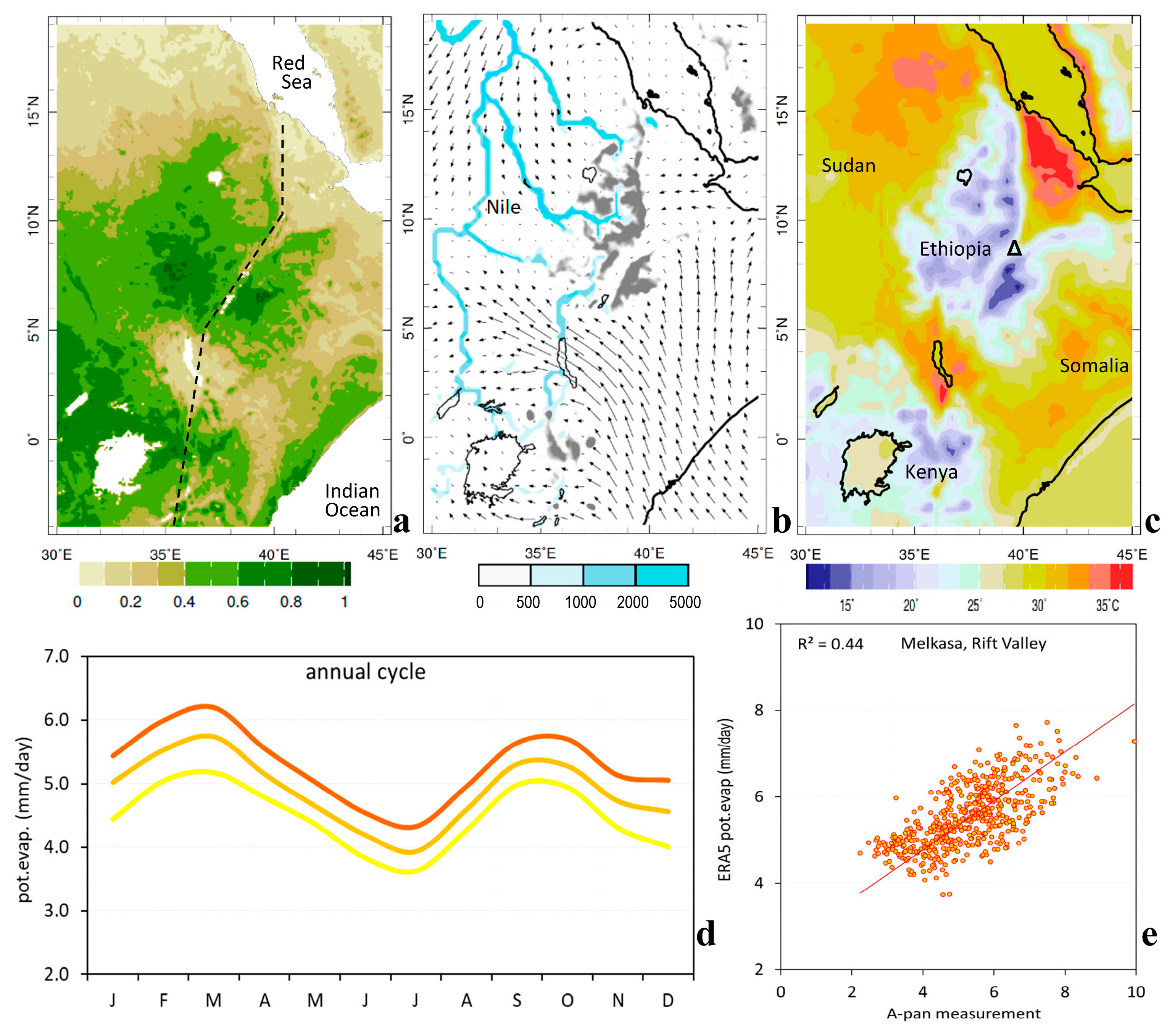
The study area includes the productive Kenya and Ethiopia highlands of NE Africa, incised by the SW–NE Rift Valley and Turkana Channel (Figure 1a–c, 4 S–19 N and 30–45 E). NE Africa is surrounded by the Sahara Desert to the northwest, the equatorial Congo forests to the southwest, and the Indian Ocean to the east. Numerous rivers (e.g., Nile) flow out of these highlands, and many large lakes sustain local resources for a growing population of ~100 M.
3. Results
3.1. Climatology and PC Modes
The 30-year climatologies for vegetation fraction, 850 hPa wind and river discharge, and surface air temperature are presented in Figure 1a–c. The maps show cool green highlands encircled by warm arid lowlands. Equatorial winds from southeast squeeze into the Turkana Channel, while subtropical winds from northeast penetrate the upper Nile confluence. The highlands naturally slow and split low-level winds, while monsoon reversals average out the longshore airflow on the coast.
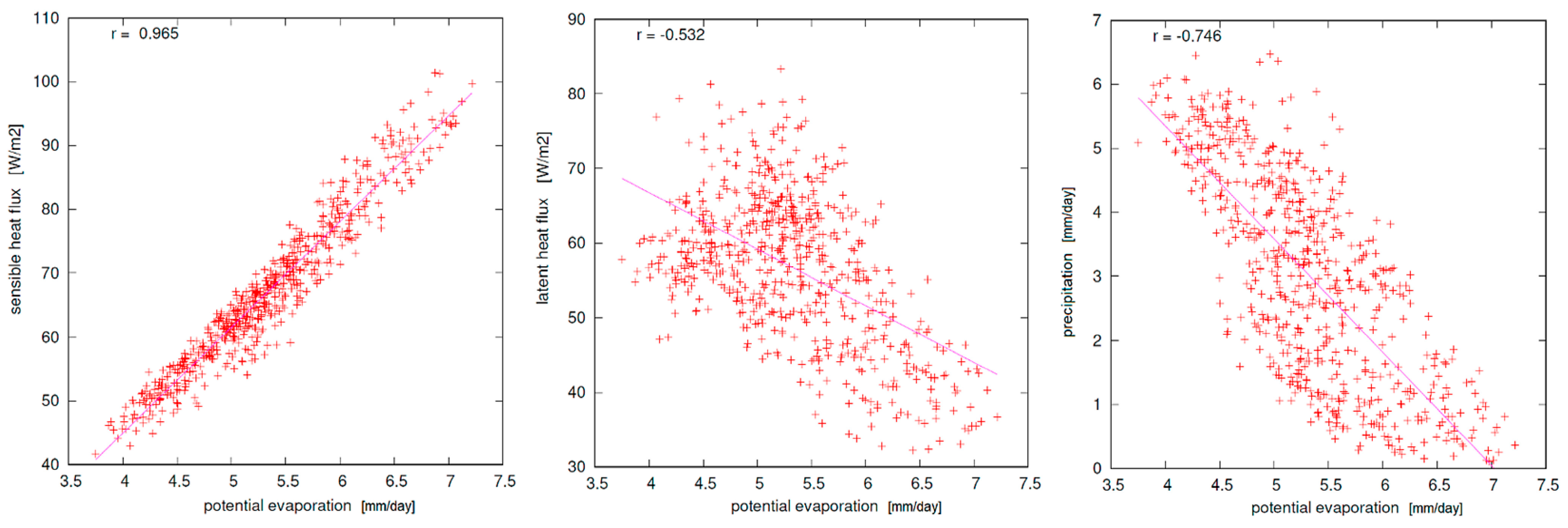
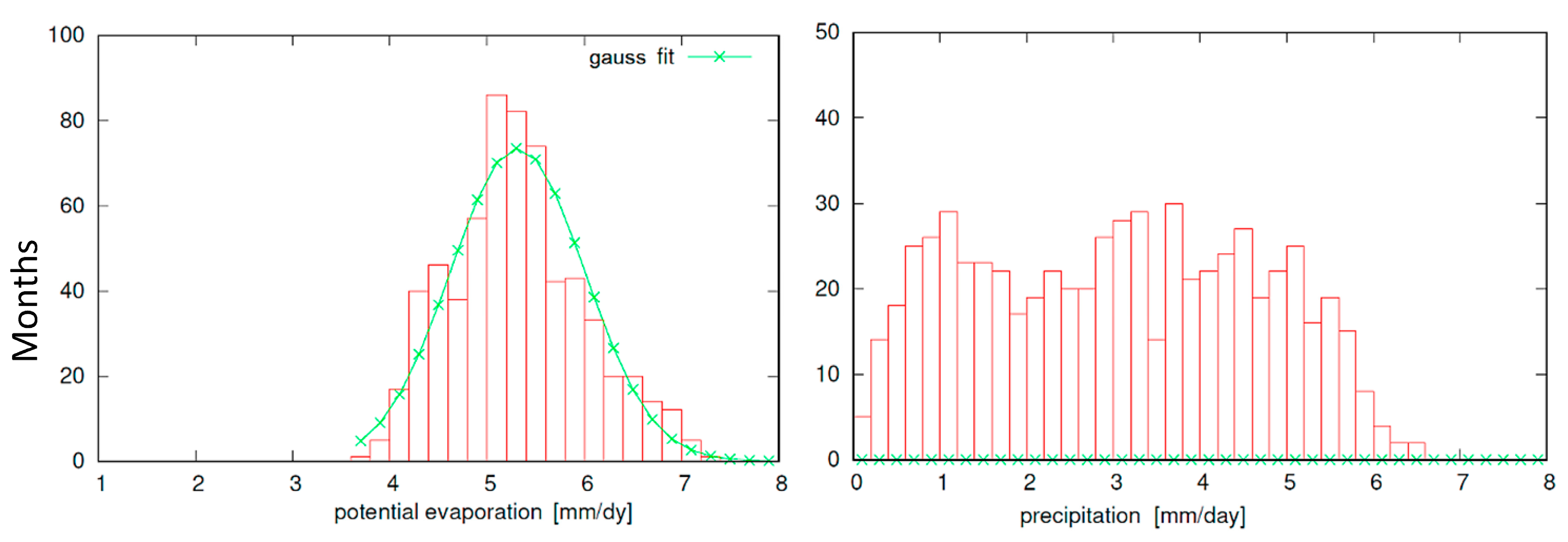
The mean annual cycle of PE in the Rift Valley (Figure 1d) exhibits a bi-modal character >5 mm/day in February–March and September–October, preceding the wet seasons. Total and anomaly cross-correlations (Rt Ra) with unfiltered PE time series for 1970–2022 are as follows: Rt + 0.97 Ra + 0.91 with SHF, Rt − 0.53 Ra − 0.78 with latent heat flux, and Rt − 0.75 Ra − 0.88 with precipitation in the Rift Valley (cf. Figure A2). The probability distribution of unfiltered PE has a Gaussian fit unlike that of rainfall (cf. Figure A3). The ~1:1 fit of ERA5 PE and SHF informs how the model derives this critical variable. The in situ measurements of A-pan potential evaporation at Melkasa (8.42 N, 39.35 E, and 1550 m) are compared with co-located monthly unfiltered ERA5 PE in Figure 1e. The scatterplot regression fit is R2 0.44, which is significant above the 99% confidence intervals, despite the comparison of grid estimate vs. point observation. Some model bias is detected below 4 mm/day (wet spells), but match-ups are good above 6 mm/day (dry spells).
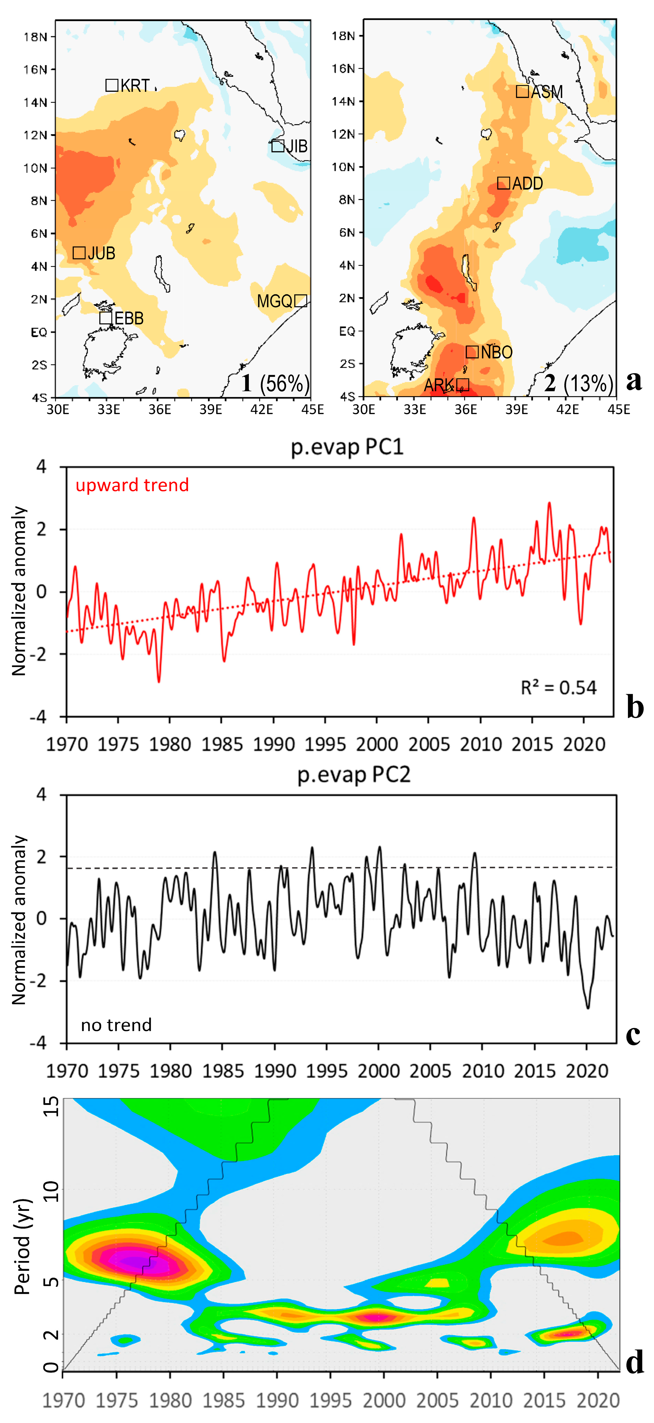
The loading patterns for ERA5 PE are presented in Figure 2a. PC-1 covers the downstream Nile Basin of Sudan; its filtered time scores (Figure 2b) show a linear rise (R2 0.54) that is attributed to global warming (Lyon 2014). PC-2 follows the Rift Valley from Tanzania (4 S) to the Red Sea (15 N), extending across the bimodal/unimodal climate regimes [3]. The filtered PC-2 time scores exhibit no obvious trend (Figure 2c,d), but the wavelet spectra have persistent oscillations at the 3.3 yr interval of 1980–2010 and the 6.3 yr interval before 1980/after 2010. Such rhythms correspond with coupled Rossby waves that propagate slowly westward in the tropical Indian Ocean [27].
3.2. Composite Drought
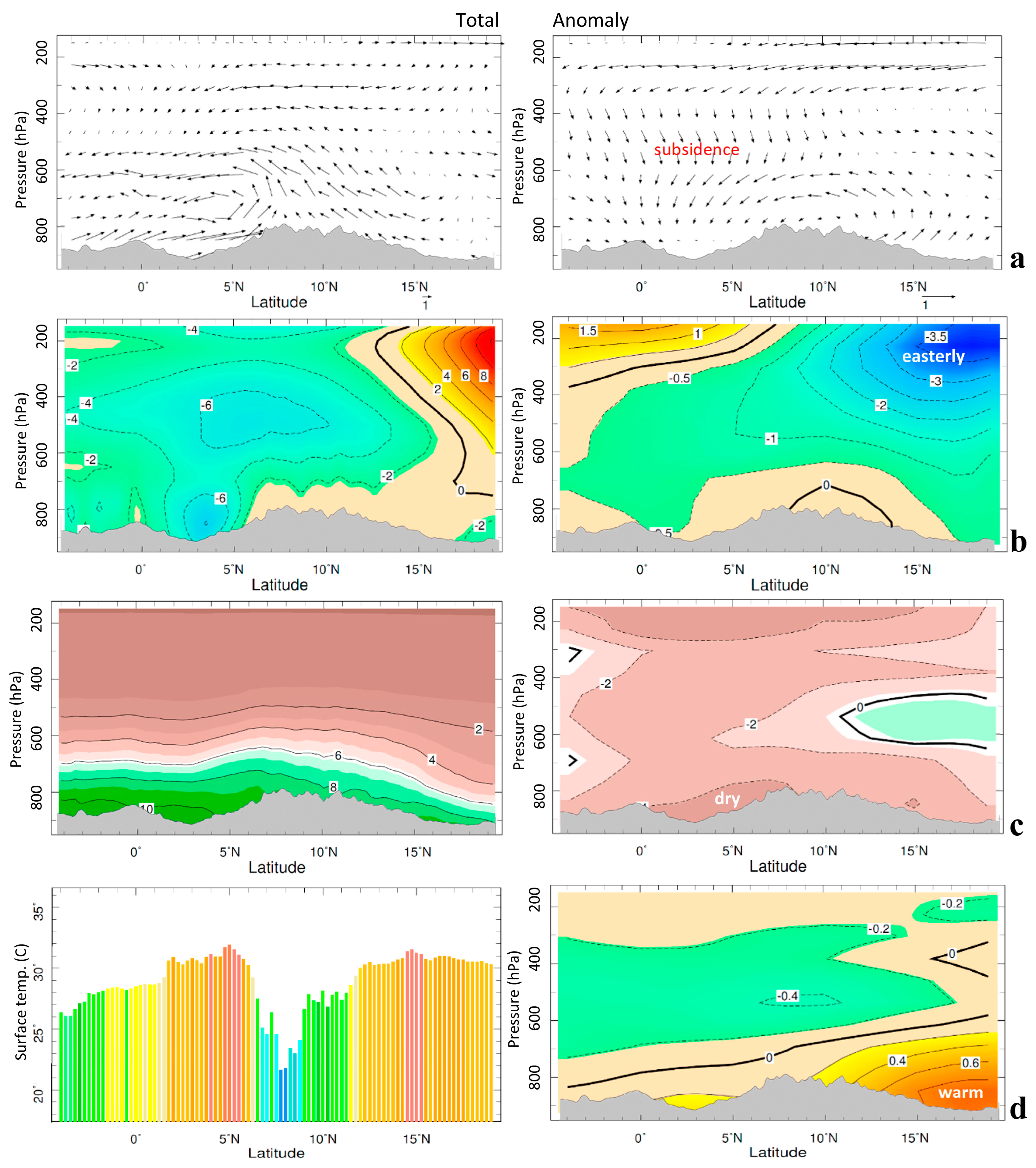
NE African drought composites were calculated for 28 dry months (Table 1) based on PC-2 PE departures > 1.6σ. Figure 3a–d illustrates the N–S sections over the Rift Valley for total and anomalous atmospheric circulation and thermodynamic condition. Starting with totals, the meridional circulation shows a marked uplift toward the Ethiopian highlands from the rotary cells on either side. The Turkana cell (4 N) is shallow and exhibits inflow/outflow at 850/600 hPa. The zonal circulation is westward, particularly in the Turkana Channel and in the mid-levels from 4 to 10 N, so humidity from the Congo Basin does not reach the Rift Valley [28]. Total air temperatures in the composite drought exceed 30 °C at 5 N and 15 N. Considering the anomalous patterns, the meridional circulation is southward and subsident in the layer 300–600 hPa, embedded within westward airflow that is prominent at 15 N 200 hPa (Figure 3a,b). Near-surface air temperatures are warmer than usual at 15 N, suggesting airmass intrusion from the arid subtropics (Figure 3c,d).
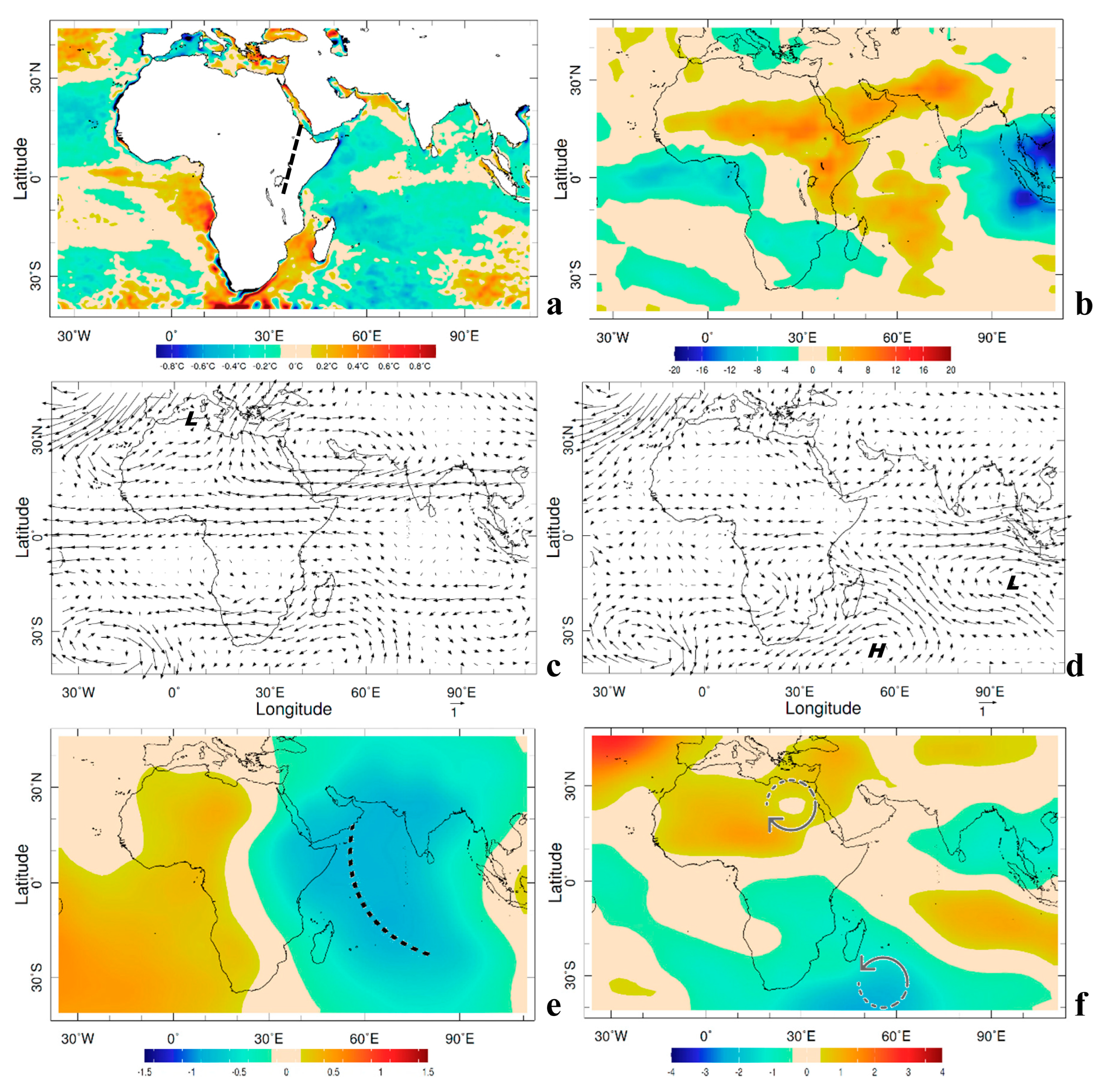
The regional composite maps offer a wider perspective in Figure 4a–f. Sea temperatures over the west Indian Ocean are below normal, signifying a thermocline tilted up west/down east, while SSTs around southern Africa are above normal. The OLR composite reveals a dry climate over the west Indian Ocean and northern subtropics; the two axes intersect at the Rift Valley. Mid-level wind anomalies are westward across NE and SE Africa. Low-level winds in the composite drought are from the southeast between the High and Low cells over the Indian Ocean. The patterns of velocity potential and stream function describe a divergent circulation that feeds from the Mascarene Islands to the Turkana Channel. Composite 500 hPa wind anomalies also reflect a trough over the Mediterranean Sea.
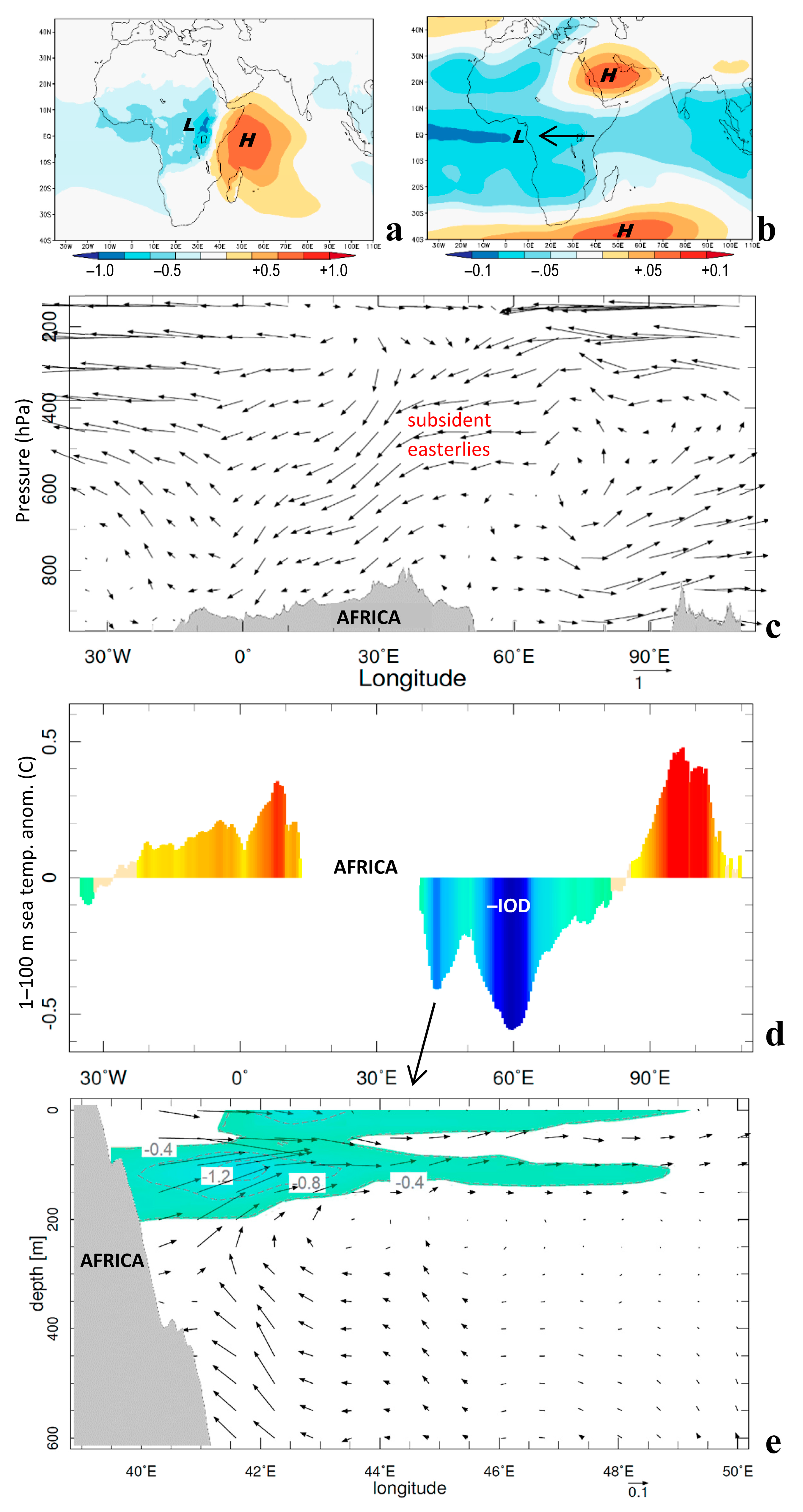
The zonal circulations are illustrated in Figure 5a–c. The regression of the PC-2 time scores onto surface air pressure and 500 hPa geopotential height reveals an E–W dipole inducing westward airflow along the equator. The height section illustrates a zonal overturning Walker Cell, similar to [12] with deep rotary motion above the central Indian Ocean. Surface winds are drawn toward the Maritime Continent and tilt the thermocline downward to the east. Upper-level airflow sinks from 250 hPa at 60 E to 600 hPa at 30 E, entraining dry air over NE Africa. Composite equatorial subsurface sea temperatures (Figure 5d) reveal a warm/cool/warm pattern at 0 E/60 E/100 E, representing negative-phase Indian Ocean Dipole (cf. Figure A1). The composite depth section of subsurface zonal circulation and sea temperature anomalies (Figure 5e) provides evidence of upwelling. During NE African drought, composite currents form a ‘conveyor’: moving coastward at depth, then rising 41–43 E, and moving seaward at the surface, thus cooling the west Indian Ocean by −1 °C.
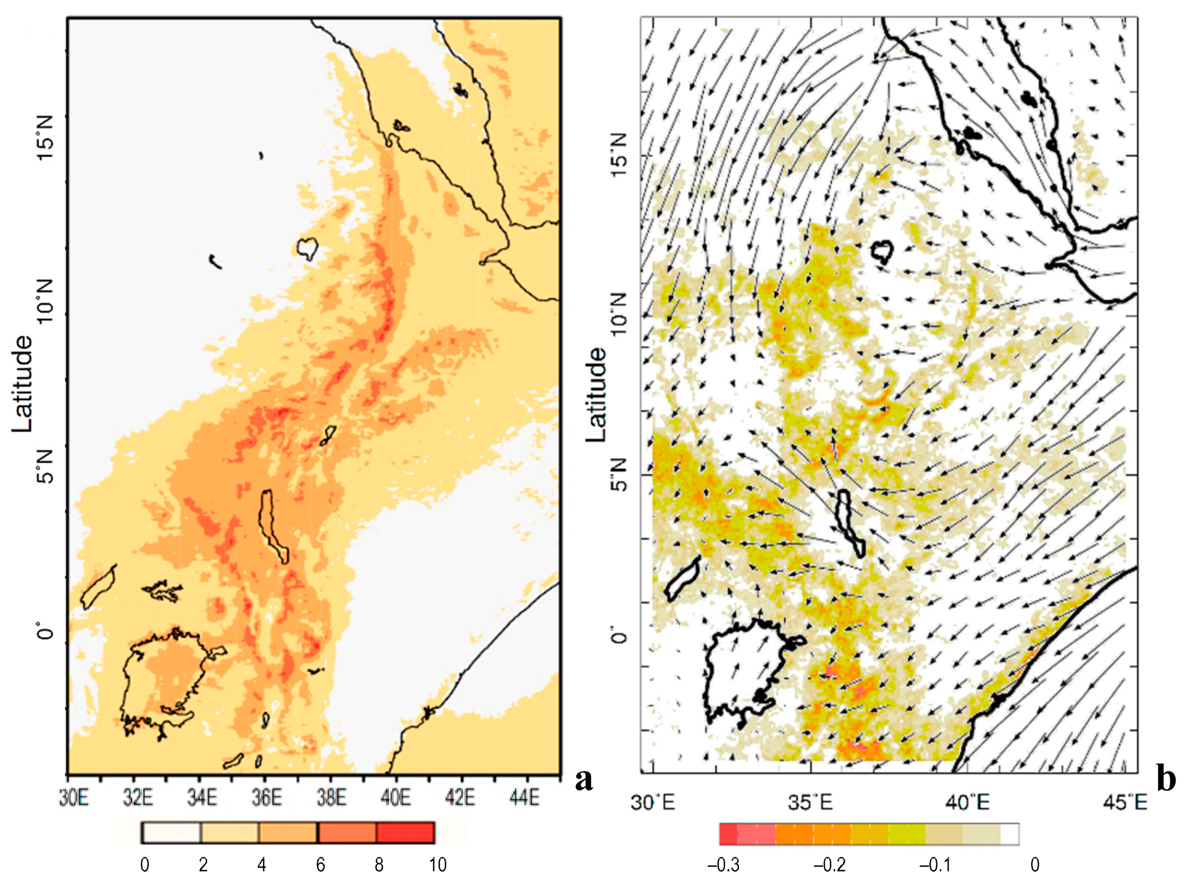
Local drought impacts (Figure 6a,b) emerge in the regression of PC-2 onto net solar radiation and in composite vegetation and wind anomalies. Increased insolation (10 W m−2/σ) follows the Rift Valley, and vegetation color fraction declines 20% under dry northeasterly airflow. The conditions on the escarpment herald negative impacts across NE Africa.
3.3. Processes and Predictability
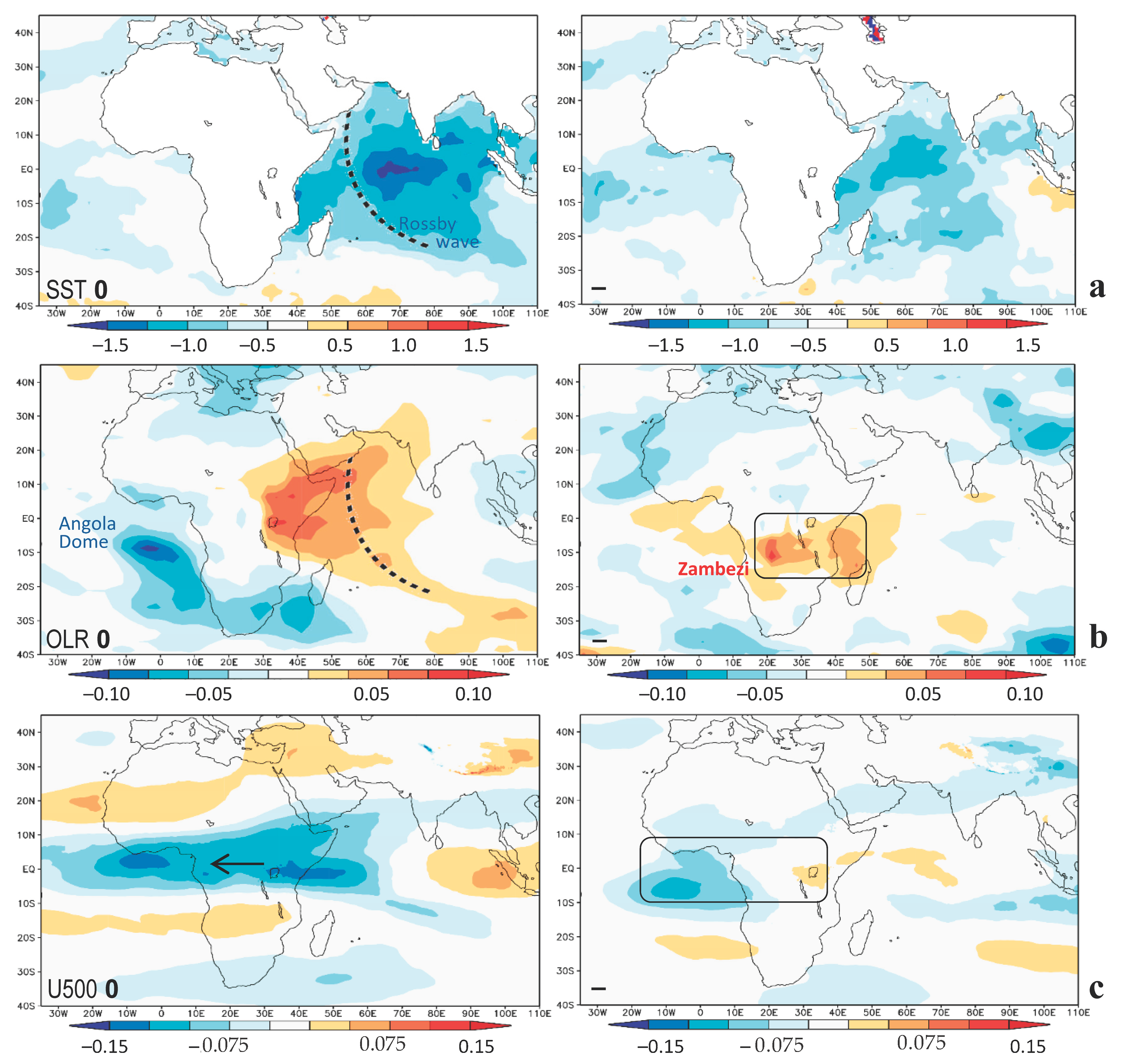
The processes and predictability underpinning NE African drought emerge from the point-to-field regression analysis (Figure 7a–c). In contrast with the composites involving 28 dry months, this method employs the entire PC-2 PE time scores (cf. Figure 2c) and reflects symmetrical and linear opposing teleconnections. The satellite SST fields show negative values representing cool conditions in the central and west Indian Ocean at 0- and 6-month lead. The <-pattern identifies an oceanic Rossby wave [29] associated with a tilted thermocline coupled with the Walker Cell. The satellite OLR regression maps indicate a 10–20° westward shift of dry weather from the zone of cool SST. During drought, atmospheric convection is active over southern Africa (−OLR). At the 6-month lead, the sign changes, and dry weather (+OLR) shifts to the Zambezi Valley/northern Madagascar (a potential predictor). The U 500 regression map shows westward airflow over the equatorial zone at the 0 lag. At the 6-month lead, this signal diminishes and shifts westward to the tropical Atlantic, offering another predictor of NE African drought.
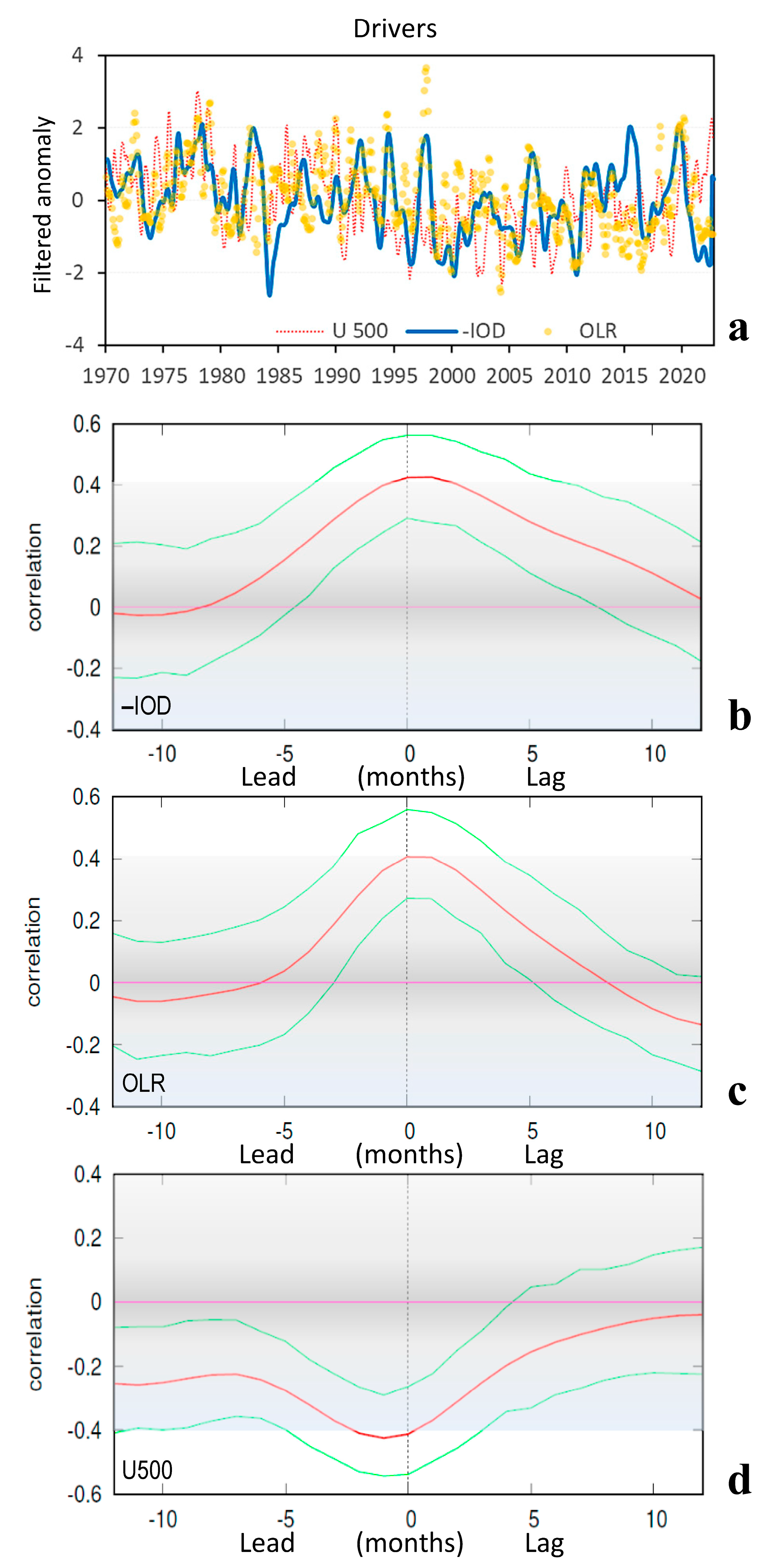
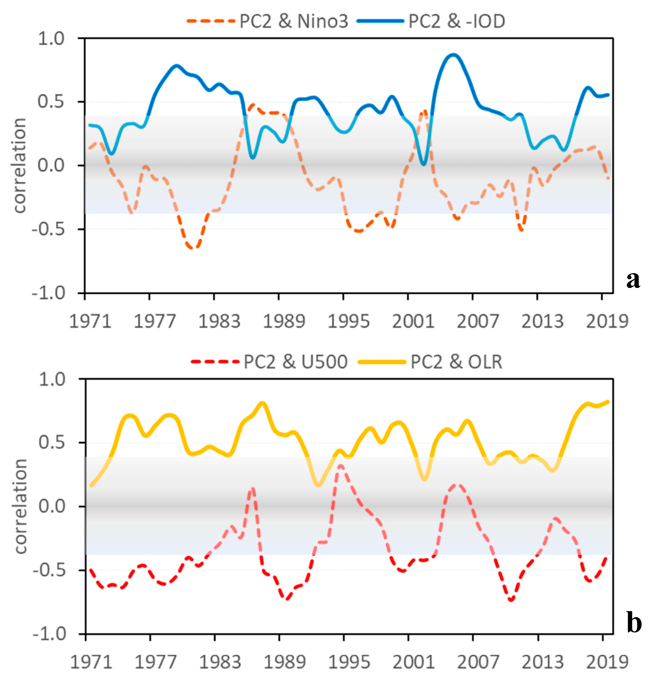
The time series of the leading drivers are plotted in Figure 8a, and lead–lag correlations are analyzed in Figure 8b–d. The OLR and U500 tend to follow −IOD, but with respect to NE African drought (PC-2), the results are statistically weak, with the lagging values barely reaching |0.4|. The multivariate regression further emphasizes the loss of predictability, covering R2 0.29 at 0 lag but only 0.07 at the 6-month lead. Figure 9a,b show the results of the investigation on why this is so, using 5-year running correlations. There are periods when the −IOD associates with the Rift Valley PE, but there are also extended spells of near-zero correlation coinciding with positive Pacific Niño3 influence. Similarly, the OLR and U500 indices sustain moderate correlation with PC-2 but decouple over three spells from 1970 to 2022. U500 winds even switch sign (like Niño3), indicating unsteady links between the Walker Cell, Pacific ENSO, and IOD.
3.4. Intra-Seasonal Variability
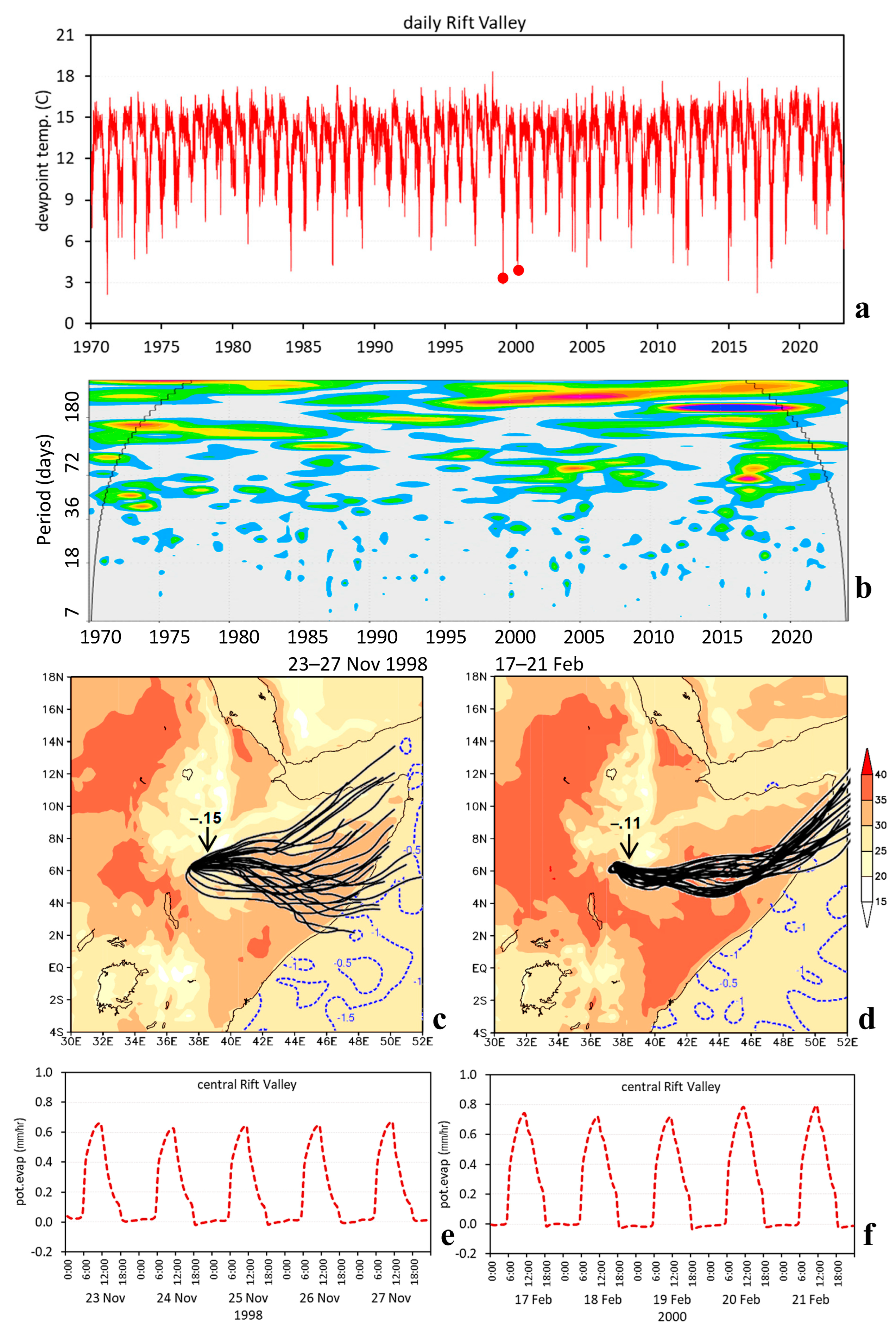
Considering intra-seasonal fluctuations, the Rift Valley daily dewpoint temperatures (Td) are plotted in Figure 10a,b. Although the values hover around 14 °C in the wet season, single digits characterize the dry season when the equatorial trough lies southward. The wavelet spectral analysis shows weak amplitudes below 36 days. There are lengthy spells of Madden Julian Oscillation influence (36–48 days), as reported by [30], and significant periods above 100 days that are indicative of prolonged climate anomalies needing mitigation. Many spells of Td < 6°C emerge, two of which occurred when the inter-annual drivers exceeded |1 σ| value during 23–27 November 1998 and 17–21 February 2000. These were analyzed for back trajectories and hourly PE, and the results are shown in Figure 10c–f. The airflow reaching the central Rift Valley during dry spells comes from Somalia, where offshore SSTs are −1°C below normal and the maximum air temperatures exceed 36°C. Subsidence is particularly strong (−0.1 m/s) as the airflow accelerates into the Turkana Channel. The hourly time series indicate arid weather conditions: diurnal PE peaks > 0.7 mm/h with SHF > 400 W/m2. The root-zone soil moisture in the Rift Valley and surrounding escarpment is depleted 50 kg/m3 during prolonged dry spells, according to the GLDAS3 estimates, yielding ~15% water content that is untenable for most crops. The lag correlations of filtered Rift Valley PE with soil moisture are significant from −1 to +3 months (Figure A4).
4. Conclusions
This study revealed new characteristics of the NE African climate via monthly ERA5 potential evaporation during 1970–2022. The methodology and results are novel because rainfall is not used to indicate drought. The outcomes based on the spatio-temporal structure were obtained from PC analysis, which leading mode in the Nile Basin exhibited an upward trend (R2 0.54), suggesting a water-stressed future. The PC-2 loading pattern followed the Rift Valley at 4 S–15 N (cf. Figure 6a) and exhibited a bimodal character, with PE showing crests before the two rainy seasons. The inter-annual fluctuations of potential evaporation correlated positively with SHF (+0.91) and negatively with rainfall and latent heat flux (−0.88, −0.79). The filtered PC-2 Rift Valley time scores contained significant spectral periods at 3.3 yr and 6.3 yr, owing to zonal oscillations of the tropical ocean thermocline [31,32].
This research tested whether NE African drought could be represented by PE in comparison with SHF and A-pan measurements. The results gave a statistically significant fit, which supported using the PC-2 time scores as a basis for exploration, thus being distinct from past research that segregated bimodal/unimodal zones and early/late summer rainfall [33]. Another unique feature was the use of subsurface sea temperatures to represent IOD (cf. Figure A1), which correlations with the Rift Valley PE were 26% better than traditional DMI SST.
The research question regarding atmosphere–ocean coupling was addressed using point-to-field regressions and composite analysis, which linked cold-phase Indian Ocean Dipole (–IOD) with zonal overturning circulation. A tilted thermocline and upwelling near the coast cooled the SST by −1 °C and thereby limited convection over NE Africa. Easterly winds subsided at −0.1 m/s, reducing dewpoint temperatures < 10 °C and desiccating vegetation. The zonal circulation exported humidity from the Congo to the Atlantic, where SST and convection were above normal.
Although this work expanded our scientific understanding, predictability remained elusive. Of the three drivers, only –IOD sustains a 6-month-lead multivariate regression, generating a paltry Rr2 of 0.07 (cf. Table 2). The teleconnections between IOD and Rift Valley PE are suppressed during spells of positive ENSO influence, pointing to unsteady coupling with the Walker Cell. Although these limit the confidence in long-range forecasts, the trends of PE over the Rift Valley have flattened since 2000, suggesting that adaptative strategies could offer benefits [34].
These results suggest that subsurface sea temperature can be used to represent IOD and PE can be used to represent drought, benefiting from its Gaussian distribution (cf. Figure A3). The outcomes further suggest that the Rift Valley amplifies diurnal heat fluxes and re-transmits drought across NE Africa. It is recommended that new weather station deployments include fast sonic anemometers with temperature to infer potential evaporation using w′T′ eddy covariance [35] for comparison with A-pan measurements.
Funding
This research received no external funding.
Data Availability Statement
A spreadsheet is available on email request.
Acknowledgments
A-pan data were derived from the Ethiopia Institute for Agriculture Research at Melkasa via A. Alaminie of Bahir Dar University. The websites used for data extraction and analysis include APDRC Univ Hawaii, IRI Climate Library, KNMI Climate Explorer, NASA–Giovanni, and NOAA Ready–ARL. The author thanks T.T. Minda of Arba Minch University for stimulating the research.
Conflicts of Interest
The author declares no conflict of interest.
Appendix A
Figure A1.
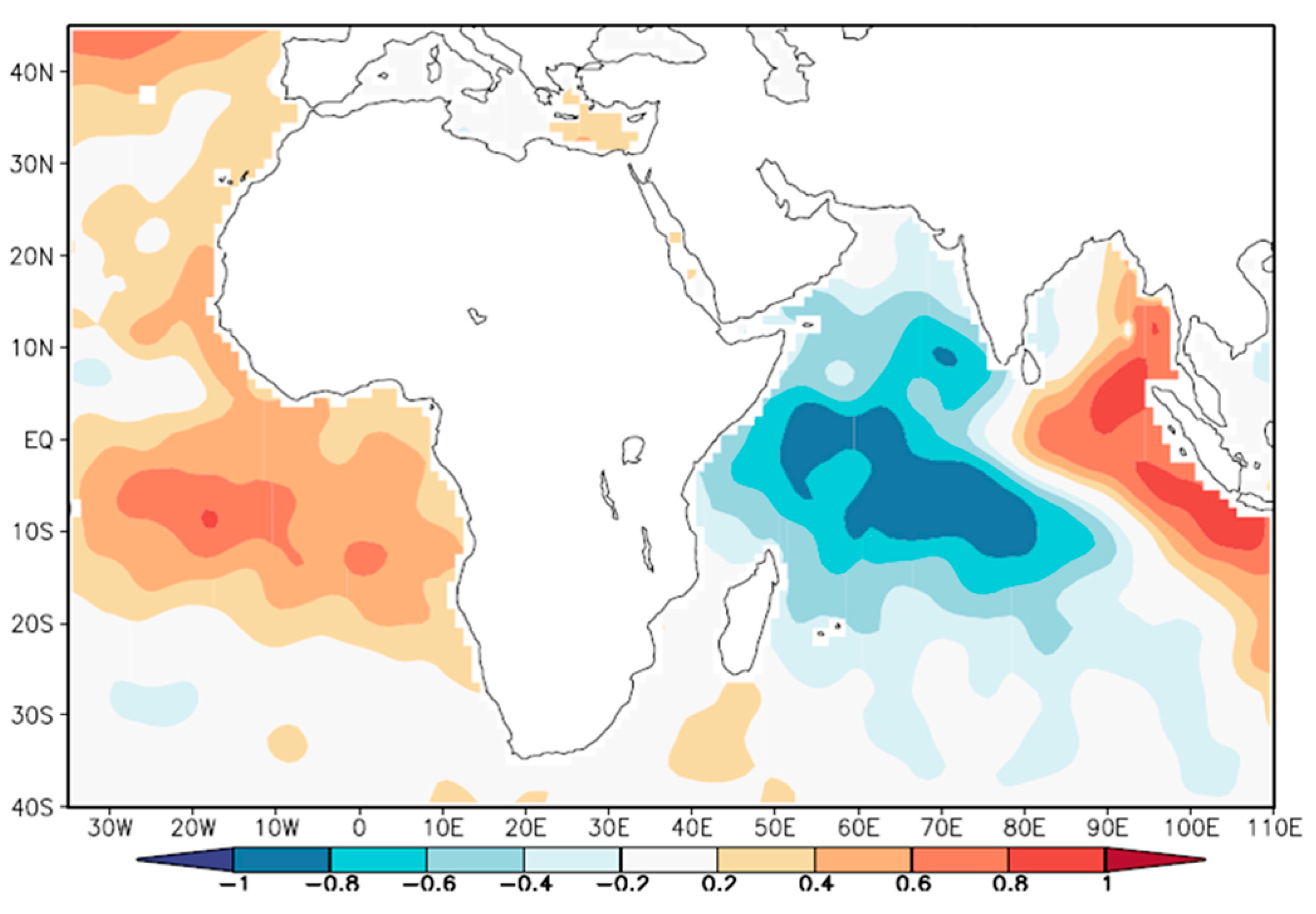
PC loading pattern of 1–100 m sea temperature representing the IOD in negative phase (associated with time scores in Figure 7a). Subsurface sea temperatures better characterize IOD: PE time score correlation with DMI of −0.16 vs. –IOD of + 0.42.
Figure A1.
PC loading pattern of 1–100 m sea temperature representing the IOD in negative phase (associated with time scores in Figure 7a). Subsurface sea temperatures better characterize IOD: PE time score correlation with DMI of −0.16 vs. –IOD of + 0.42.

Figure A2.
Scatterplots of Rift Valley unfiltered PE vs. SHF, latent heat flux, and rainfall (left to right).
Figure A2.
Scatterplots of Rift Valley unfiltered PE vs. SHF, latent heat flux, and rainfall (left to right).

Figure A3.
(left) Histogram of Rift Valley unfiltered PE, with Gaussian fit having 0.35 skewness. (right) Same histogram of Rift Valley unfiltered precipitation. N = 636 months.
Figure A3.
(left) Histogram of Rift Valley unfiltered PE, with Gaussian fit having 0.35 skewness. (right) Same histogram of Rift Valley unfiltered precipitation. N = 636 months.

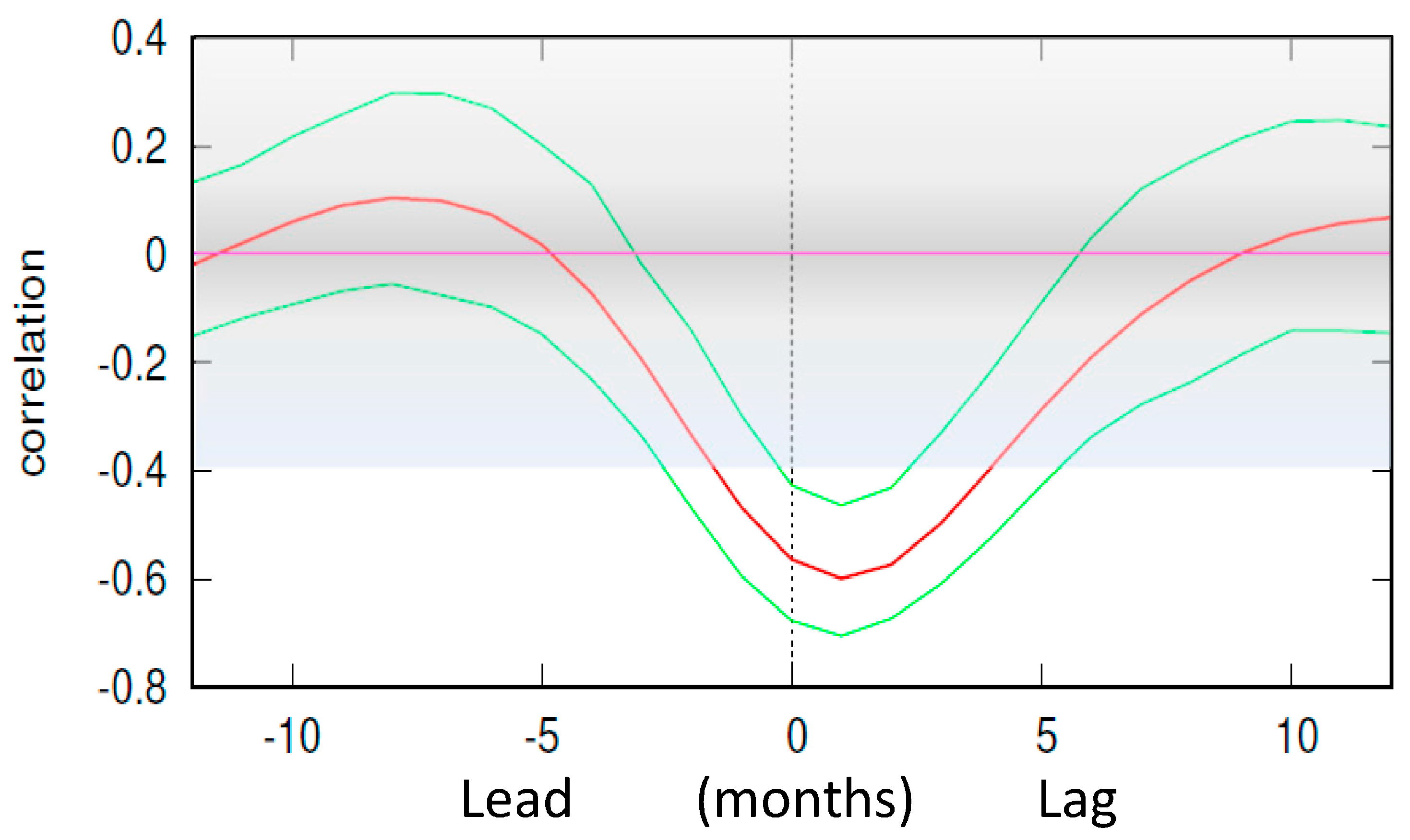
Figure A4.
Lag correlation of filtered PC-2 time scores onto Rift Valley soil moisture. A positive value refers to ERA5 PE leading GLDAS3 soil moisture, and the shading area covers R coefficients < |0.4|, as in Figure 8.
Figure A4.
Lag correlation of filtered PC-2 time scores onto Rift Valley soil moisture. A positive value refers to ERA5 PE leading GLDAS3 soil moisture, and the shading area covers R coefficients < |0.4|, as in Figure 8.

References
- Jimma, T.B.; Demissie, T.; Diro, G.T.; Ture, K.; Terefe, T.; Solomon, D. Spatiotemporal variability of soil moisture over Ethiopia and its teleconnections with remote and local drivers. Theor. Appl. Climatol. 2023, 151, 1911–1929. [Google Scholar] [CrossRef]
- Camberlin, P.; Fontaine, B.; Louvet, S.; Oettli, P.; Valimba, P. Climate adjustments over Africa accompanying the Indian Monsoon onset. J. Clim. 2010, 23, 2047–2064. [Google Scholar] [CrossRef]
- Nicholson, S.E. Climate and climatic variability of rainfall over eastern Africa. Rev. Geophys. 2017, 55, 590–635. [Google Scholar] [CrossRef]
- Owiti, Z.; Ogallo, L.; Mutemi, J. Linkages between the Indian Ocean Dipole and East African rainfall anomalies. J. Kenya Meteo. Soc. 2008, 2, 3–17. [Google Scholar]
- Molla, M. Teleconnections between ocean-atmosphere coupled phenomenon and droughts in northern Ethiopia. Am. J. Clim. Chang. 2020, 9, 274–296. [Google Scholar] [CrossRef]
- Vizy, E.K.; Cook, K.H. Observed relationship between the Turkana low-level jet and boreal summer convection. Clim. Dyn. 2019, 53, 4037–4058. [Google Scholar] [CrossRef]
- Jury, M.R.; Minda, T.T. Turkana low-level jet influence on southwest Ethiopia climate. J. Hydrometeorol. 2023, 24, 585–599. [Google Scholar] [CrossRef]
- Lyon, B. Seasonal drought in the greater Horn of Africa and its recent increase during the March–May long rains. J. Clim. 2014, 27, 7953–7975. [Google Scholar] [CrossRef]
- Rowell, D.P.; Booth, B.B.; Nicholson, S.E.; Good, P. Reconciling past and future rainfall trends over East Africa. J. Clim. 2015, 28, 9768–9788. [Google Scholar] [CrossRef]
- Funk, C.; Hoell, A.; Shukla, S.; Blade, I.; Liebmann, B.; Roberts, J.B.; Husak, G. Predicting East African spring droughts using Pacific and Indian Ocean sea surface temperature indices. Hydrol. Earth Syst. Sci. 2014, 18, 4965–4978. [Google Scholar] [CrossRef]
- Funk, C.; Harrison, L.; Shukla, S.; Pomposi, C.; Galu, G.; Korecha, D.; Husak, G.; Magadzire, T.; Davenport, F.; Hillbruner, C.; et al. Examining the role of unusually warm Indo-Pacific sea-surface temperatures in recent African droughts. Q. J. R. Meteorol. Soc. 2018, 144, 360–383. [Google Scholar] [CrossRef]
- Liebmann, B.; Bladé, I.; Funk, C.; Allured, D.; Quan, X.-W.; Hoerling, M.; Hoell, A.; Peterson, P.; Thiaw, W.M. Climatology and interannual variability of boreal spring wet season precipitation in the eastern Horn of Africa and implications for its recent decline. J. Clim. 2017, 30, 3867–3886. [Google Scholar] [CrossRef]
- Jury, M.R. South Indian Ocean Rossby waves. Atmos. Ocean. 2018, 56, 322–331. [Google Scholar] [CrossRef]
- Hastenrath, S. Zonal circulations over the equatorial Indian Ocean. J. Clim. 2000, 13, 2746–2756. [Google Scholar] [CrossRef]
- Hoell, A.; Funk, C. Indo-Pacific sea surface temperature influences on failed consecutive rainy seasons over eastern Africa. Clim. Dyn. 2014, 43, 1645–1660. [Google Scholar] [CrossRef]
- Hersbach, H.; Bell, B.; Berrisford, P.; Hirahara, S.; Horányi, A.; Muñoz-Sabater, J.; Thépaut, J.N. The ERA5 global reanalysis. Q. J. R. Meteorol. Soc. 2020, 146, 1999–2049. [Google Scholar] [CrossRef]
- Adem, A.; Aynalem, D.; Tilahun, S.; Steenhuis, T. Predicting reference evaporation for the Ethiopian Highlands. J. Water Res. Prot. 2017, 9, 1244–1269. [Google Scholar] [CrossRef]
- Singer, M.B.; Asfaw, D.T.; Rosolem, R.; Cuthbert, M.O.; Miralles, D.G.; MacLeod, D.; Quichimbo, E.A.; Michaelides, K. Hourly potential evapotranspiration at 0.1° resolution for the global land surface from 1981-present. Sci. Data 2021, 8, 224. [Google Scholar] [CrossRef] [PubMed]
- Saha, S.; Moorthi, S.; Wu, X.; Wang, J.; Nadiga, S.; Tripp, P.; Behringer, D.; Hou, Y.-T.; Chuang, H.-Y.; Iredell, M.; et al. The NCEP climate forecast system version 2. J. Clim. 2014, 27, 2185–2208. [Google Scholar] [CrossRef]
- Rodell, M.; Houser, P.R.; Jambor, J.U. The Global Land Data Assimilation System. Bull. Amer. Meteor. Soc. 2004, 85, 381–394. [Google Scholar] [CrossRef]
- Um, M.-J.; Kim, Y.; Park, D.; Jung, K.; Wang, Z.; Kim, M.M.; Shin, H. Impacts of potential evapotranspiration on drought phenomena in different regions and climate zones. Sci. Total Environ. 2020, 703, 135590. [Google Scholar] [CrossRef] [PubMed]
- Wang, Y.; Wang, S.; Zhao, W.; Liu, Y. The increasing contribution of potential evapo-transpiration to severe droughts in the Yellow River basin. J. Hydrol. 2022, 605, 127310. [Google Scholar] [CrossRef]
- Jury, M.R. Representing the Indian Ocean Dipole. Phys. Oceanogr. 2022, 29, 417–432. [Google Scholar]
- Mueller, R.; Matsoukas, C.; Gratzki, A.; Behr, H.; Hollmann, R. The CM-SAF operational scheme for the satellite based retrieval of solar surface irradiance. Remote Sens. Environ. 2009, 113, 1012–1024. [Google Scholar] [CrossRef]
- Carton, J.A.; Chepurin, G.A.; Chen, L. SODA-3 a new ocean climate reanalysis. J. Clim. 2018, 31, 6967–6983. [Google Scholar] [CrossRef]
- Stein, A.F.; Draxler, R.R.; Rolph, G.D.; Stunder, B.J.B.; Cohen, M.D.; Ngan, F. NOAA’s HYSPLIT atmospheric transport and dispersion modeling system. Bull. Am. Meteorol. Soc. 2015, 96, 2059–2077. [Google Scholar] [CrossRef]
- Yamagata, T.; Behera, S.K.; Luo, J.-J.; Masson, S.; Jury, M.R.; Rao, S.A. Coupled Ocean–Atmosphere Variability in the Tropical Indian Ocean. In Earth Climate: Ocean–Atmosphere Interaction; Wang, C., Xie, P.P., Carton, J.A., Eds.; American Geophysical Union: USA, 2003; pp. 189–212. Available online: https://ftp.cpc.ncep.noaa.gov/hwang/OLD/Yamagata_2004_GR.pdf (accessed on 1 June 2022).
- Viste, E.; Sorteberg, A. Moisture transport into the Ethiopian highlands. Int. J. Climatol. 2013, 33, 249–263. [Google Scholar] [CrossRef]
- Jury, M.R.; Huang, B. The Rossby wave as a key mechanism of Indian Ocean climate variability. Deep. Sea Res. Part I Oceanogr. Res. Pap. 2004, 51, 2123–2136. [Google Scholar] [CrossRef]
- Vellinga, M.; Milton, S.F. Drivers of interannual variability of the East African long rains. Q. J. R. Meteorol. Soc. 2018, 144, 861–876. [Google Scholar]
- Yeshanew, A.; Jury, M.R. North African climate variability, part 1: Tropical thermocline–coupling. Theor. Appl. Climatol. 2007, 89, 25–36. [Google Scholar] [CrossRef]
- Yeshanew, A.; Jury, M.R. North African climate variability, part 2: Tropical circulation systems. Theor. Appl. Climatol. 2007, 89, 37–49. [Google Scholar] [CrossRef]
- Palmer, P.I.; Wainwright, C.M.; Dong, B.; Maidment, R.I.; Wheeler, K.G.; Gedney, N.; Hickman, J.E.; Madani, N.; Folwell, S.S.; Abdo, G.; et al. Drivers and impacts of Eastern African rainfall variability. Nat. Rev. Earth Environ. 2023, 4, 254–270. [Google Scholar] [CrossRef]
- Wainwright, C.M.; Marsham, J.H.; Keane, R.J.; Rowell, D.P.; Finney, D.L.; Black, E.; Allan, R.P. Eastern African paradox, rainfall decline due to shorter not less intense long rains. Clim. Atmos. Sci. 2019, 2, 34. [Google Scholar] [CrossRef]
- Mauder, M.; Jegede, O.O.; Okogbue, E.C.; Wimmer, F.; Foken, T. Surface energy balance measurements at a tropical site in West Africa during the transition from dry to wet season. Theor. Appl. Climatol. 2007, 89, 171–183. [Google Scholar] [CrossRef]
Figure 1.
Long-term mean maps: (a) satellite vegetation color fraction with the Rift Valley shown as a dashed line; (b) ERA5 850 hPa winds (largest 10 m/s) with grey highlands > 2000 m elevation and blue river discharge (m3/s); (c) ERA5 surface air temperature; (d) Rift Valley mean annual cycle and terciles of monthly PE; and (e) scatterplot of Melkasa (Δ in c) A-pan measurements (×0.7) vs. co-located monthly ERA5 PE and linear regression.

Figure 2.
(a) PC loading patterns (shaded blue −1 σ to red +1 σ) with labeled mode (variance) and capital cities □ with airport codes. (b) Potential evaporation PC-1 (Nile Basin) time scores with linear regression. (c) Potential evaporation PC-2 (Rift Valley) time scores, and (d) its wavelet spectrum with the 90–98% confidence intervals shaded, and period in log scale with the cone of validity; the temporal analyses have been normalized and 6-month filtered; and the dashed line in (c) is the composite threshold.

Figure 3.
N–S height sections at 35–40 E for composite drought: left—total and right—anomalies for (a) meridional circulation (m/s), (b) zonal wind (m/s), (c) specific humidity (g/kg), and (d) temperature (°C), with topographic profile overlain on top, using the months listed in Table 1. Total temperature (lower left) illustrates surface values along the Rift Valley.

Figure 4.
Regional maps of composite drought anomalies for (a) SST (°C), (b) OLR (W/m2), (c) 500 hPa wind (vector m/s), (d) 850 hPa wind (vector m/s), (e) 500 hPa velocity potential (106 m2/s), and (f) 850 hPa streamfunction (106 m2/s), using the months listed in Table 1. The Rift Valley is shown by dashed line in (a), the curved dashed line represents the axis of divergent circulation in (e) and rotational airflow is given by icon in (f).

Figure 5.
Regression of filtered PC-2 (PE) time scores onto fields of (a) surface air pressure (/hPa) and (b) 500 hPa geopotential height (/m) with icons. Equatorial 10 N–10 S sections of composite drought: (c) zonal atmospheric circulation anomaly (Walker Cell), (d) equatorial 1–100 m sea temperature anomalies along 35 W–110 E, and (e) depth section of zonal circulation and temperature anomalies in the coastal sector with shelf profile.

Figure 6.
(a) Regression of PC-2 time scores onto EC satellite net solar radiation (W m–2/σ). (b) Composite drought satellite vegetation anomaly (shaded < 0) and surface wind (largest vector of 2 m/s), using the months listed in Table 1.
Figure 6.
(a) Regression of PC-2 time scores onto EC satellite net solar radiation (W m–2/σ). (b) Composite drought satellite vegetation anomaly (shaded < 0) and surface wind (largest vector of 2 m/s), using the months listed in Table 1.

Figure 7.
Regression of filtered PC-2 (PE) time scores onto fields at 0- and 6-month lead (right): (a) SST (/°C), (b) OLR (/W m−2), and (c) U500 hPa wind (/m s−1) with arrow highlighting airflow. Oceanic Rossby wave is shown as a dashed line on the left in (a,b), and index areas are outlined on the right in (b,c).

Figure 8.
(a) Time series of leading drivers. Lag correlation of PC-2 time scores onto the following variables: (a) –IOD index, (b) OLR index, and (c) U 500 wind index. A negative value refers to a driver leading the PC-2 PE time scores, with all scores being normalized and 6-month filtered, and the shading area covers R coefficients < |0.4|. The loading pattern for the –IOD index is illustrated in Figure A1.

Figure 9.
Simultaneous 5-year running correlation of PC-2 PE time scores with (a) Niño3 SST and –IOD index, and (b) OLR and U500 indices, with all scores being 6-month filtered. The shading area covers R coefficients < |0.4|.
Figure 9.
Simultaneous 5-year running correlation of PC-2 PE time scores with (a) Niño3 SST and –IOD index, and (b) OLR and U500 indices, with all scores being 6-month filtered. The shading area covers R coefficients < |0.4|.

Figure 10.
(a) Daily time series of Rift Valley dewpoint temperatures, showing two cases (dots) when all drivers exceeded |1 σ| (cf. Table 1), and (b) the wavelet spectral analysis shaded from the 90–98% confidence intervals, in log scale with the cone of validity. Hysplit back trajectories arriving at 6 N, 37.25 E, and 1000 m in the central Rift Valley: (c) 23–27 November 1998 and (d) 17–21 February 2000. ERA5 maximum air temperature (shaded), low-level subsidence (arrow m/s), and NOAA SST anomalies < −0.5 °C (blue dashed). (e,f) Hourly PE time series in the central Rift Valley, based on CFS2 sensible heat flux.


Table 1.
Ranked dates of Rift Valley potential evaporation PC-2 time score > 1.6 σ used in composites. Successive dry groups include February–June 1984, June–October 1993, October 1998–January 1999, November 1999–April 2000, and January–May 2009. Standardized 6-month filtered variables are listed, and the two dry cases are denoted with *.
| Year | Month | PC2 | –IOD | OLR | U500 |
|---|---|---|---|---|---|
| 2000 | 2 * | 2.32 | 1.99 | 1.98 | −1.60 |
| 1993 | 8 | 2.30 | 1.10 | −0.10 | −0.22 |
| 2000 | 1 | 2.23 | 1.78 | 1.90 | −1.37 |
| 2000 | 3 | 2.18 | 2.10 | 1.60 | −1.55 |
| 1993 | 9 | 2.15 | 1.26 | 0.28 | −0.21 |
| 1984 | 4 | 2.15 | 2.50 | 0.57 | −0.55 |
| 1984 | 3 | 2.12 | 2.63 | 1.13 | −1.05 |
| 2009 | 4 | 2.12 | 0.38 | 1.07 | −0.72 |
| 1993 | 7 | 2.12 | 0.78 | −0.32 | −0.20 |
| 2009 | 3 | 2.11 | 0.47 | 1.01 | −1.27 |
| 1999 | 12 | 2.04 | 1.57 | 1.42 | −1.24 |
| 1984 | 5 | 2.01 | 2.23 | −0.09 | 0.13 |
| 1998 | 11 * | 2.00 | 1.71 | 1.53 | −1.57 |
| 2009 | 5 | 1.95 | 0.23 | 1.15 | −0.38 |
| 1998 | 10 | 1.93 | 1.67 | 1.57 | −1.13 |
| 2009 | 2 | 1.93 | 0.49 | 0.90 | −1.53 |
| 1998 | 12 | 1.84 | 1.73 | 1.26 | −1.70 |
| 1993 | 6 | 1.83 | 0.48 | −0.26 | −0.32 |
| 1984 | 2 | 1.79 | 2.55 | 0.99 | −1.13 |
| 1999 | 11 | 1.78 | 1.38 | 1.15 | −1.34 |
| 2002 | 7 | 1.76 | 0.02 | −0.25 | −1.86 |
| 2000 | 4 | 1.76 | 2.07 | 0.96 | −1.21 |
| 1984 | 6 | 1.72 | 1.94 | −0.57 | 0.29 |
| 1990 | 8 | 1.71 | 0.35 | 0.73 | −1.53 |
| 2009 | 1 | 1.68 | 0.44 | 0.67 | −1.61 |
| 2002 | 6 | 1.68 | 0.13 | 0.37 | −1.81 |
| 1993 | 10 | 1.65 | 1.32 | 0.49 | −0.05 |
| 1999 | 1 | 1.64 | 1.73 | 0.99 | −1.67 |
Table 2.
Multivariate regression of three variables onto the filtered PC-2 time scores (potential evaporation): (a) simultaneous and (b) 6-month lead, 1970–2022.
Table 2.
Multivariate regression of three variables onto the filtered PC-2 time scores (potential evaporation): (a) simultaneous and (b) 6-month lead, 1970–2022.
| Statistics (0 lead) | ||||||
|---|---|---|---|---|---|---|
| Adj. R sq. | 0.295 | |||||
| Std. Error | 0.840 | |||||
| ANOVA | ||||||
| df | SS | MS | F | Sign. F | ||
| Regression | 3 | 188.16 | 62.72 | 88.86 | 7 × 10–48 | |
| Residual | 626 | 441.84 | 0.706 | |||
| Total | 629 | 630.00 | ||||
| Coeff. | Std. Error | t Stat | p–value | −95% | +95% | |
| Intercept | 0.009 | 0.034 | 0.276 | 0.783 | −0.057 | 0.075 |
| –IOD | 0.247 | 0.039 | 6.285 | 0.000 | 0.170 | 0.324 |
| U500 | −0.291 | 0.036 | −8.133 | 0.000 | −0.361 | −0.221 |
| OLR | 0.189 | 0.040 | 4.759 | 0.000 | 0.111 | 0.267 |
| (a) | ||||||
| Statistics (6-month lead) | ||||||
| Adj. R sq. | 0.070 | |||||
| Std. Error | 0.967 | |||||
| ANOVA | ||||||
| df | SS | MS | F | Sign. F | ||
| Regression | 3 | 46.49 | 15.50 | 16.58 | 2.3 × 10⁻¹⁰ | |
| Residual | 620 | 579.53 | 0.935 | |||
| Total | 623 | 626.02 | ||||
| Coeff. | Std. Error | t Stat | p–value | −95% | +95% | |
| Intercept | 0.006 | 0.039 | 0.158 | 0.875 | −0.070 | 0.082 |
| –IOD | 0.272 | 0.046 | 5.925 | 0.000 | 0.182 | 0.362 |
| U500 | −0.063 | 0.042 | −1.501 | 0.134 | −0.145 | 0.019 |
| OLR | −0.041 | 0.046 | −0.891 | 0.373 | −0.131 | 0.049 |
| (b) | ||||||
Disclaimer/Publisher’s Note: The statements, opinions and data contained in all publications are solely those of the individual author(s) and contributor(s) and not of MDPI and/or the editor(s). MDPI and/or the editor(s) disclaim responsibility for any injury to people or property resulting from any ideas, methods, instructions or products referred to in the content. |
© 2023 by the author. Licensee MDPI, Basel, Switzerland. This article is an open access article distributed under the terms and conditions of the Creative Commons Attribution (CC BY) license (https://creativecommons.org/licenses/by/4.0/).
Share and Cite
MDPI and ACS Style
Jury, M.R. Characterizing Northeast Africa Drought and Its Drivers. Climate 2023, 11, 130. https://doi.org/10.3390/cli11060130
AMA Style
Jury MR. Characterizing Northeast Africa Drought and Its Drivers. Climate. 2023; 11(6):130. https://doi.org/10.3390/cli11060130
Chicago/Turabian StyleJury, Mark R. 2023. "Characterizing Northeast Africa Drought and Its Drivers" Climate 11, no. 6: 130. https://doi.org/10.3390/cli11060130
Note that from the first issue of 2016, this journal uses article numbers instead of page numbers. See further details here.