Study of Turbulence Associated with the Faraji Cyclone

Abstract

The formation of a cyclonic region in which nonlinear interactions generate turbulence in the form of small-scale vortices can be observed because of the different rotating air masses. Turbulence dynamics in cyclones (specifically hurricanes) has been under-researched; therefore, assessing the shear term is crucial to identify the onset of cyclonic formation within a region of the atmosphere. Earth observation techniques are able to provide relevant information on this physical process. In this article, we propose a new framework that is useful for connecting the study of the dynamics of a cyclonic system with the observations generated by geostationary satellite facilities. In particular, we applied the proper orthogonal decomposition (POD), a technique widely used in turbulent analysis to decompose a generic scalar or vector field in empirical eigenfunction, to investigate a tropical cyclone, the Faraji hurricane, from a dynamic point of view, beginning from the temporal evolution of its temperature field. The latter was obtained by elaborating on data and images collected by the SEVIRI radiometer, installed on the Meteosat Second Generation-8 (IODC) satellite. Using the POD, the energy spectra of both the spatial and temporal components of the temperature field obtained through remote sensing techniques were studied separately. Important information was then extracted and used for an in-depth characterization of the properties of the turbulence in the non-linear evolution of this phenomenon.

1. Introduction

Cyclones are extreme atmospheric conditions that have significantly contributed, over the course of time, to the evolution of climate change and its impact on the Earth’s system. It is well known [1] that cyclone events are triggered by high temperature air masses following a rotational motion developed around a low pressure center. They are driven by a strong thermal source, which continuously supplies energy in the form of latent heat, so they generate spiral motions of the atmosphere, causing rotational dynamics in the geographic region concerned. These events are mainly formed in tropical latitudes; hence, the name tropical cyclones. According to their speeds of motion, they assume particular characteristic conditions; moreover, they are cataloged in classes of strength, according to the Saffir–Simpson scale [1,2]. A hurricane is defined as a tropical cyclone that has reached the highest class, corresponding to category 5.

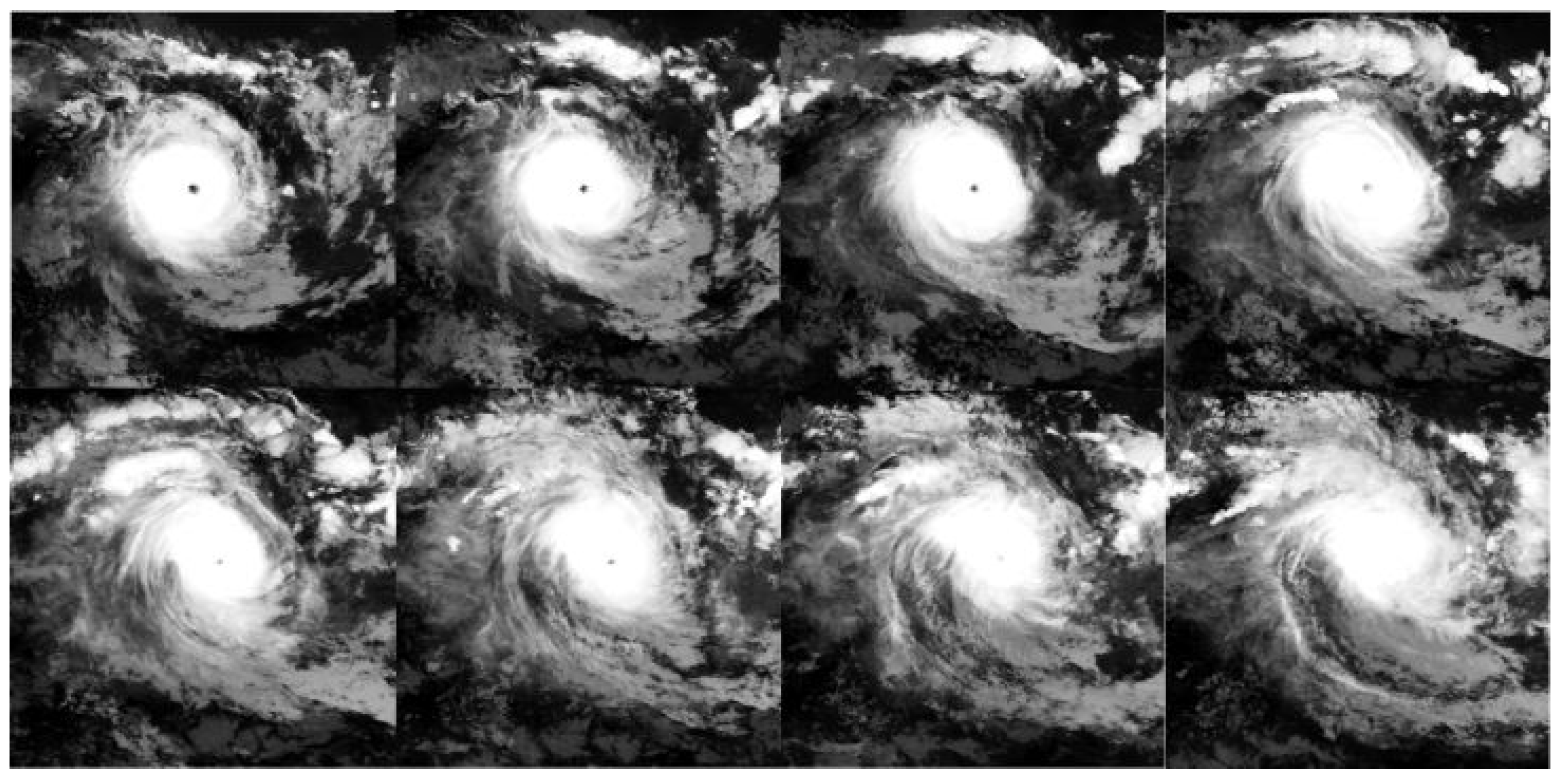
The strong pressure differences among air masses rotating around the low pressure center generates turbulence in the surrounding regions [3,4,5]. In this work, we studied the characteristic properties of turbulence at different spatiotemporal scales within the regions of hurricane Faraji, the first tropical cyclone of the 2021 season that reached category 5 on the Saffir–Simpson scale; it developed in the Indian Ocean between 4 and 13 February 2021. We would like to point out that the word “turbulence” is used hereinafter in the generic sense of “random superposition of different length scales”. The actual mechanisms that can produce this small-scale formation (turbulent cascade, local instabilities, convection, etc.) are not explored in detail in our investigation. The study uses data and imagery collected by the SEVIRI radiometer [6], installed on the Meteosat Second Generation-8 (IODC) (MSG-8), an EUMETSAT geostationary satellite. With these products, remote sensing techniques were used to obtain a series of N images, made of matrices of $N_{\mathrm{lon}}\times N_{\mathrm{lat}}$ pixels, where $N_{\mathrm{lon}}$ and $N_{\mathrm{lat}}$ are, respectively, the resolution in longitude and latitude, in a given period of acquisition. Each pixel (representing a total area of 1 Km ${}^2$ for SEVIRI) is assigned a brightness temperature value, so that the image is a matrix representing the temperature field of the cyclone observed at a given time. Starting from this scalar field, we carried out the analysis of the spatiotemporal dynamics of cyclones using the proper orthogonal decomposition (POD) technique [7,8,9,10]. Thus, the original field was decomposed on the basis of empirical eigenfunctions extracted directly from the data by diagonalizing the autocorrelation matrix of the temperature field, integrated on the whole domain (Fredholm problem of the second kind). The spatial and temporal components were factorized in the POD expansion by attributing the spatial dependency to the eigenfunctions and the temporal evolution to the coefficients of the development.

The POD technique has several advantages over other traditional techniques (such as Fourier or Wavelet analyses): (a) it does not assume any special behavior at the boundaries of the domain; (b) the empirical basis is optimal, in the sense that it captures (on average) the maximum possible energy on each mode, which means that the POD spectrum has the most rapid decrease as a function of the discrete number of the eigenfunctions; (c) the POD eigenfunctions are orthonormal and the temporal coefficients are decorrelated from each other. When studying turbulent motions, especially in the non-homogeneous case, the POD decomposition acquires a special value, as it is well known that turbulence in shear layers is characterized by the presence of “coherent structures”, namely energy-containing, velocity field structures that persist in the flow for several nonlinear turnover times. As a consequence of the property (b), the POD eigenfunctions in this framework are correlated with the turbulent coherent structures. In the case of statistically homogeneous isotropic turbulence, the coherent structures are plane waves; in fact, the POD decomposition applied to the periodic fields yields, as a result, the Fourier expansion.

However, concerning differences with expansions in which the basis is fixed a priori, as with the Fourier or Wavelet decompositions, no characteristic scale can be intrinsically associated directly with the POD eigenfunctions, in the sense that each eigenfunction does not have, in principle, a single characteristic scale, but it may be composed of many of them, all mixed together. Moreover, since the basis is extracted empirically directly from the data, the energy spectra of two different datasets cannot be easily compared directly, since the eigenfunctions themselves, and not only the coefficients, contain the information concerning the energetic budget.

Through the POD analysis, and from the analysis of the spectra, we infer that the turbulent dynamics of cyclones appear to be characterized by three different slopes of the spectra, at three different ranges of characteristic scales that we call macroscale, mesoscale, and small-scale, each one likely associated to different atmospheric properties within the cyclone and characterized by a different evolution.

The remainder of the manuscript is structured as follows. In the following section, we briefly describe the technique used for obtaining the data through a remote sensing analysis and, hence, we recall the main properties of the POD decomposition, which will be used throughout the rest of the article. Then, we present the results of the analysis carried out on the Faraji cyclone. Finally, we present our conclusions and outlooks from the present study.

2. Materials and Methods

We used satellite remote sensing techniques that allowed us to observe the evolution of the cyclone, beginning from a series of images acquired from MSG-8, using the SEVIRI radiometer. The number of images used in the current study was $N=93$: the Faraji cyclone was observed over a total period of 23 h, in steps of 15 min. Each of the 93 images represents a snapshot of the temperature field T as a matrix of pixels $\Delta R=N_{\mathrm{lon}}\times N_{\mathrm{lat}}$, in which data were inserted in digital number (DN) units.

In the case under study, $N_{\mathrm{lon}}=350$ and $N_{\mathrm{lat}}=350$ pixels, respectively, and each pixel represents an area of 1 Km ${}^2$. Some of these images of the Faraji hurricane are shown in Figure 1. In this figure, the temperature fields, obtained through remote sensing analysis techniques, are shown at different times in intervals of 21 h from 12:00 UTC on 8 February to 09.00 UTC on 9 February, 2021. The time sequence is shown in intervals of 3 h each.

2.1. Remote Sensing Analysis

The remote sensing analysis consisted of the following process: for each raw image, from the DN data we obtained the radiance recorded at sensor $L_{\lambda }$, defined as a linear function of the image DN values:

$$L_{\lambda }=f\left(DN\right)=gDN+b$$

(1)

in which the values g and b represent calibration parameters, called gain and offset, respectively, extracted from the ancillary data of the terrestrial receiving stations. The radiance is expressed in units W·m ${}^{-2}·$sr${}^{-1}·\mathsf{\mu }$m${}^{-1}$, and is integrated for each pixel on the entire wavelength bandwidth of the channel [11,12].

Using the ITT ENVI software, we applied Equation (1) to obtain N images, in which the values assigned to the pixels are in radiance units. From these new images, we used Planck’s law as a relationship that links the radiance L to brightness temperature $T_b$ [13]:

$$L_{\lambda }=\frac{2h{c}^2{\lambda }^{-5}{ϵ}_{\lambda }}{(e^{\frac{hc}{k\lambda T_b}}-1)}$$

(2)

where $\lambda$ is the wavelength, h is the Planck’s constant, c is the speed of light, ${ϵ}_{\lambda }$ is the emissivity, and k the Boltzmann constant.

Inverting (2) and setting ${ϵ}_{\lambda }=1$ (unitary emissivity), we obtain:

$$T_b=\frac{hc{\left(k\lambda \right)}^{-1}}{ln\left(\frac{2h{c}^2{\lambda }^{-5}}{L_{\lambda }}+1\right)}$$

(3)

In this expression, the brightness temperature $T_b$ is in Kelvin units (K) and the wavelength $\lambda$ represents the central one in the spectral channel bandwidth from which the information is extracted. In this analysis, we consider the thermal infrared (TIR) spectral channel, whose central wavelength is $\lambda =10.8\mathsf{\mu }$m.

2.2. Proper Orthogonal Decomposition Analysis

A homogeneous and isotropic turbulent signal, produced by the dynamics of a fluid, can be studied using a Fourier decomposition approach [7,8,9]. However, when we study a turbulent fluid that is neither homogeneous nor isotropic, the Fourier analysis in normal modes does not produce optimal results. In fact, in such cases, the most energetic structures of the flow are not “plane waves”, in the Fourier sense, but they assume the form of localized structures, which are dynamically created in time during the evolution of the flow. Such structures, often called “coherent structures” [14,15,16,17], can survive for relatively long times, interact with the surrounding medium, and are subsequently destroyed and created again. Such a continuous process of creation–evolution–destruction of energetic structures (generally identified as the process of “ejection–sweep–burst”) brings an effective energy dissipation in the flow, and is responsible, for instance, for the lack of rate flow in ducts.

In such non-homogeneous, non-isotropic situations, one can take advantage of the characteristics of the proper orthogonal decomposition (POD) technique (see, for instance, [18,19,20], and references therein). This approach, which has been widely employed in the study of the turbulent evolution of inhomogeneous flows, has been applied over time to other fields of investigation, in which the temporal evolution of a generic quantity, not necessarily “turbulent”, but with a complicated structure, was the subject of study [7,8,9,10]. In the present article, we applied the technique to study the turbulent structures obtained from the temporal evolution of the temperature field extracted through a remote sensing analysis of the satellite images of the Faraji hurricane.

We first consider a set of snapshots of a field $T_k=T(x,y,t_k)$, defined on a generic point $(x,y)\in \Omega$, where $\Omega$ is the spatial domain, at certain discrete times $t_k$. In our case, the field T represents the $2D$ discrete map of the brightness temperature of the Faraji hurricane at a particular time of observation, but in general, it can be any n-dimensional ($n=1,2,3$) scalar or vector field, depending on the space and time coordinates. We look for a decomposition of such fields into an “optimal” basis, directly extracted from the data (therefore an empirical basis) for this system, described through a denumerable set of functions $\left\{{\varphi }_j(x,y)\right\}$, such that the fields are represented in the form:

$$T(x,y,t_k)=\sum _j{a}_j\left(t_k\right){\varphi }_j(x,y)$$

(4)

where $a_j\left(t\right)$ are time-dependent modal coefficients and ${\varphi }_j(x,y)$ are basis functions that only depend on space variables. In this way, the spatial dynamics are factorized from the temporal ones and the evolution of the two can be separately evaluated.

The basis functions ${\varphi }_j(x,y)$ are obtained as the solutions of the following eigenvalue problem (Fredholm integral equation):

$${\int }_{\Omega }d{x}^{\prime }d{y}^{\prime }<T(x,y,t_k)T^{*}(x^{\prime },y^{\prime },t_k){>}_{t_k}{\varphi }_j(x^{\prime },y^{\prime })={\lambda }_j{\varphi }_j(x,y)$$

(5)

where the average $<·{>}_{t_k}$ is calculated on the ensemble of snapshots of the field at the generic time $t_k$. Therefore, the “optimal” basis is given by the eigenfunctions ${\varphi }_j$ of Equation (5), whose nucleus is associated with the averaged autocorrelation function $R(x^{\prime },y^{\prime },x,y)=<T(x^{\prime },y^{\prime },t_k)T^{*}(x,y,t_k){>}_{t_k}$. For the experimental dataset under consideration, the R operator is self-adjoint, compact, and non-negative. From this, one infers that the eigenfunctions ${\varphi }_j$ are orthogonal (each to the other) and that the eigenvalues ${\lambda }_j$, besides being real, are also “positive definite” and represent the time-averaged energy content of the j-th POD mode.

From the Fredholm Equation (5), we find an infinite number of real and positive eigenvalues ${\lambda }_j$ and the same infinite number of real eigenfunctions ${\varphi }_j$ (mutually orthogonal to each other in space). This property of orthogonality allows one to compute the partial sums on the spatiotemporal components of the field, to reconstruct it by keeping in account the contributions of a given interval of scales $[s_{\mathrm{init}},s_{\mathrm{final}}]$, only:

$$T_s(x,y,t_k)=\sum _{s_{\mathrm{init}}\le j\le s_{\mathrm{final}}}{a}_j\left(t_k\right){\varphi }_j(x,y)$$

(6)

We again emphasize the fact that, at differences, with respect to the Fourier development case, the empirical eigenfunctions ${\varphi }_j$ are, in principle, not associated with any particular spatial scale. However, we will show throughout the rest of the article that it is possible to associate characteristic spatial scales to such functions as well as characteristic time scales to the coefficients.

In this work, we applied the POD to separately analyze the spatial and temporal dynamics of the Faraji cyclone, starting from the brightness temperature field $T_b$ (hereinafter referred to as T) obtained from satellite products derived from Equation (3). In particular, it can be seen that, when the analysis is applied to a finite set of discrete times $\left\{t_k\right\}$, the generic sum over the j index appearing into Equation (4) can be truncated to the number N of independent snapshots analyzed:

$$T(x,y,t_k)=\sum _{j=1}^N{U}_j\left(t_k\right)R_j(x,y)$$

(7)

where $\left\{R_j(x,y)\right\}$ is the basis of POD eigenfunctions obtained empirically from the data, and $U_j\left(t\right)$ are the empirical coefficients that provide the temporal evolution of the field.

As described in Section 1, the temperature field T is obtained for each of the $N=93$ images, expressed as pixel matrices $\Delta R=N_{\mathrm{lon}}\times N_{\mathrm{lat}}$. The total number of pixels in both longitude and latitude is 350, so that $\Delta R=350\times 350=\mathrm{122,500}$ pixels, with each pixel representing an area $A=1$ Km${}^2$. The number N of images produced for Faraji corresponds to the number of time instants of acquisition. We obtain an observation of the dynamic evolution of the cyclone along a total period of $t=23$ h, in steps of $\Delta t=15$ min.

We previously wrote a numerical code [7,9,18] to solve the Fredholm problem given by Equation (5) and to find the eigenfunctions ${\varphi }_j$, the eigenvalues ${\lambda }_j$, and the coefficients $a_j$ of the POD development. In the present work, we applied the analysis to the temperature field, in which x and y are the coordinates associated with longitude and latitude on the surface of Earth, respectively. This produces a set of eigenfunctions $R_j(x,y)$ and a set of correspondent coefficients $U_j\left(t\right)$, associated with the sequence of eigenvalues ${\lambda }_j$ (with $j=0,1,\dots ,93$), which represent the time-average of the energy contained in the j-th POD mode, sorted in descending order. However, due to the optimality condition, not all eigenvalues are worth being considered in the analysis. A generally accepted criterion [18,19] used to select the most meaningful eigenfunctions and eigenvalues is to only consider the number of eigenvalues (ordered in decreasing order of energy content) whose sum contains at least $99\%$ of the average energy. According to this criterion, in the following, we considered only the contribution of the $M=70$ most energetic eigenvalues. The contribution of the remaining $1\%$ of the average energy is well above the estimated instrumental error ($\sim 0.1\%$) on the temperature measurements, as reported in the detailed characteristics of SEVIRI [6]. Moreover, with the temperature being a positive-definite dataset, we subtracted from each snapshot of the temperature $T(x,y,t_k)$ the time average of the field $<T(x,y,t_k){>}_{t_k}$, in such a way that the analysis was performed only on the temperature fluctuations with respect to this average.

In the last phase of the POD analysis procedure, we exploited the orthogonality property of the extracted eigenfunctions, which allowed reconstructing the temperature field inside the cyclone at different spatial scales. To do this, we used the partial sums in Equation (6).

3. Results

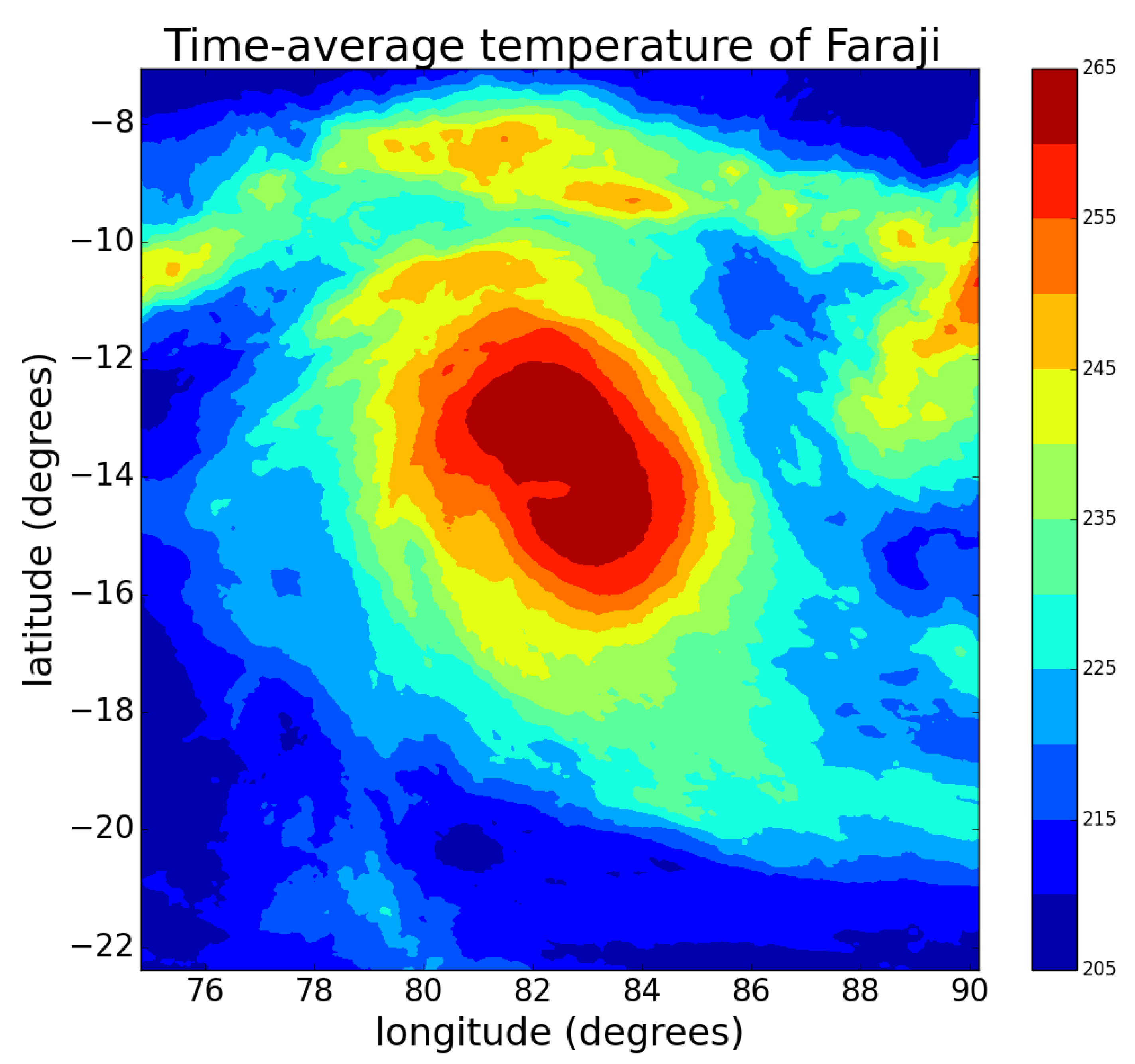
In Figure 2, we show a contour plot of the time-averaged temperature field $<T{>}_{t_k}$, as a function of the $(x,y)$ (latitude and longitude) coordinates, to have a physical representation of the average structure of hurricane Faraji. The hotter central zone coincides with the “eye” of the cyclone, surrounded by colder zones. One can notice that high-temperature spots are however present, not only in the middle of the domain, but also in the upper part of it, yielding a complicated picture of the structure of this hurricane.

To analyze the existence of a direct relationship between the order j of the POD eigenfunctions and the spatial scales—not defined a-priori because the order of the eigenfunction is connected to the energy content of the mode, not to the characteristic scales—we calculated the Fourier spectrum, shell-integrated in the wave vector space $(k_x,k_y)$, for each snapshot of the temperature field. To this aim, we computed the two-dimensional fast Fourier transform (FFT), of the temperature field. Then we divided the $(k_x,k_y)$ plane into two-dimensional concentric circular regions (shells). The i-th shell had an internal radius equal to $k^{\left(\mathrm{int}\right)}$ and an external radius equal to $k^{\left(\mathrm{ext}\right)}$. The width of all the shells was therefore equal to $\Delta k=|k^{\left(\mathrm{ext}\right)}-k^{\left(\mathrm{int}\right)}|$. Then, we attributed the i-th shell with a spectral energy equal to the sum of the energies corresponding to values of $(k_x,k_y)$, such that: $\left|k\right|=\sqrt{k_x^2+k_y^2}$, with $k^{\left(\mathrm{int}\right)}\le \left|k\right|<k^{\left(\mathrm{ext}\right)}$. Then, we computed all contributions of energy coming from different shells as a function of $\left|k\right|$. 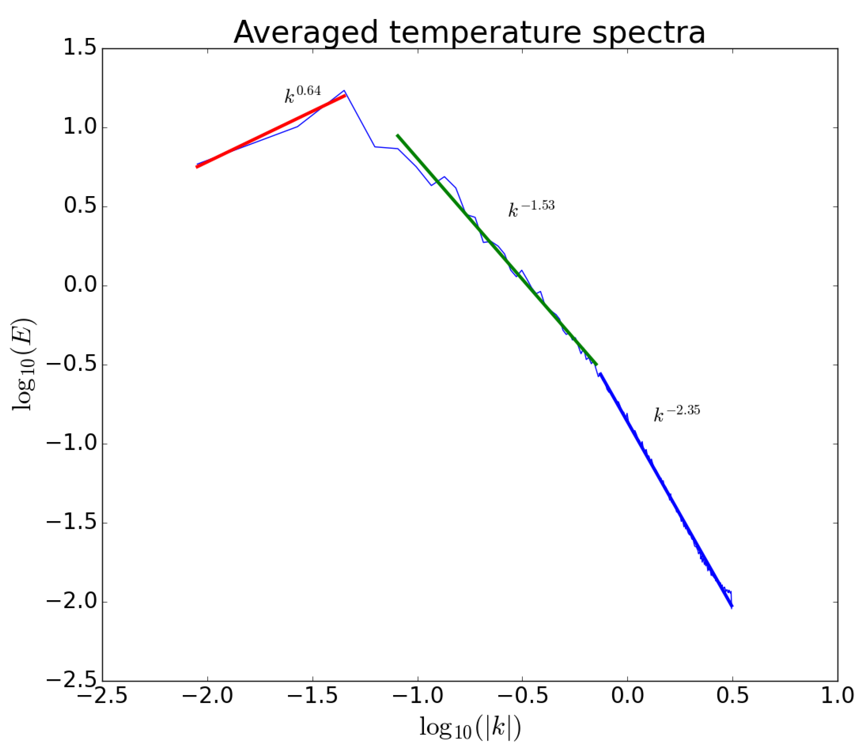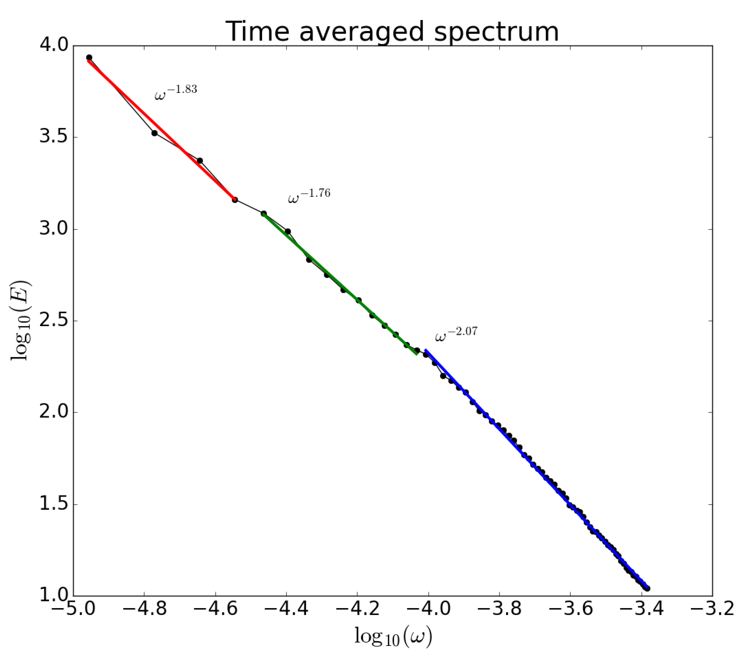Finally, the shell-integrated spectrum was averaged at the different times, to evaluate the mode energy content in the dynamics factorizing the spatial dependence. We plotted this spectrum for the Faraji cyclone in Figure 3.

From the plot in Figure 3, one can observe that the spectrum exhibits three distinct slopes; thus, allowing us to make a first classification of the spatial dependency of the eigenfunctions into three different zones, which we associate to three corresponding ranges of characteristic scales: macroscales, mesoscales, and small-scales. Such ranges of scales correspond, according to the limits of the fits, to scales larger than ∼100 km for the macroscales, between ∼22.6 and ∼100 km for the mesoscales, and smaller than ∼22.6 km for small-scales. In the plot, we highlighted the spectral indices of the fitting power law $k^{\alpha }$ for the macroscales, mesoscales, and small-scales, which go approximately as $\alpha =0.64,-1.53,-2.35$, respectively.

The slopes of the three different zones and their limits have been determined in the following way: suppose we have a spectrum of $E\left(\right|k\left|\right)$ as a function of $\left|k\right|$, which behaves as a power law in three distinct zones (let us call them Z1, Z2, and Z3). By taking the logarithms of both E and $\left|k\right|$, the spectrum in the three zones behaves like a straight line $y\left(x\right)=\alpha x+\beta$, where y represents $logE$, x is $log\left|k\right|$, $\alpha$ is the slope of the power law, and $\beta$ is a parameter depending on the energy contained at some arbitrary value of $\left|k\right|$. In order to determine the spectral slopes and the values of $log\left|k\right|$ at which the transitions among the different zones happen, we separately consider zones Z1 and Z2 first, then zones Z2 and Z3.

We fit the first two zones with a linear function $y\left(x\right)$, defined as:

$$y\left(x\right)=\left\{\begin{array}{cc}{\alpha }_{1}x+{\beta }_1\hfill & \mathrm{when}x\le \gamma \hfill \\ {\alpha }_{2}x+{\beta }_2\hfill & \mathrm{when}x>\gamma \hfill \end{array}\right.$$

where ${\alpha }_1$ and ${\alpha }_2$ are the slopes of the two different power laws in Z1 and Z2, respectively, $\gamma$ is the value where the change in the slope between the two zones takes place, and ${\beta }_1$ and ${\beta }_2$ are the constant parameters of the straight line fits. By imposing that the two linear functions are to match their values at $x=\gamma$, we can see that not all the parameters are independent. Therefore, we can express one of those parameters, for instance, ${\alpha }_2$, as a function of the remaining ones (for instance, ${\alpha }_1$, $\gamma$, and ${\beta }_{1,2}$ in this case). This can be obtained through the relation:

$${\alpha }_2={\alpha }_1-({\beta }_2-{\beta }_1)/\gamma$$

(8)

By substituting this relation in the expression of $y\left(x\right)$, the final form of the fitting function is:

$$y\left(x\right)=\left\{\begin{array}{cc}{\alpha }_{1}x+{\beta }_1\hfill & \mathrm{when}x\le \gamma \hfill \\ \left({\alpha }_1-\frac{{\beta }_2-{\beta }_1}{\gamma }\right)x+{\beta }_2\hfill & \mathrm{when}x>\gamma \hfill \end{array}\right.$$

(9)

Finally, we fit the quantities: $logE$ versus $log\left|k\right|$ in Z1 and Z2 against the function defined in Equation (9). This is a four-parameter fit, which yields the values of the slope ${\alpha }_1$, the value $x=\gamma$ where the change in the slope happens, and the parameters ${\beta }_1$ and ${\beta }_2$, as well as the value of the slope in the second zone ${\alpha }_2$ through the relation (8).

After determining the slopes and the break in the spectrum in zones Z1 and Z2, we repeat the procedure for zones Z2 and Z3, to find the slope in Z3 (the one in Z2 is of course the same obtained in the first part of the procedure) and the second spectral break. This procedure gave us the values of $\alpha$ and the point in which the separation among macro-, meso-, and small-scales takes place, described above.

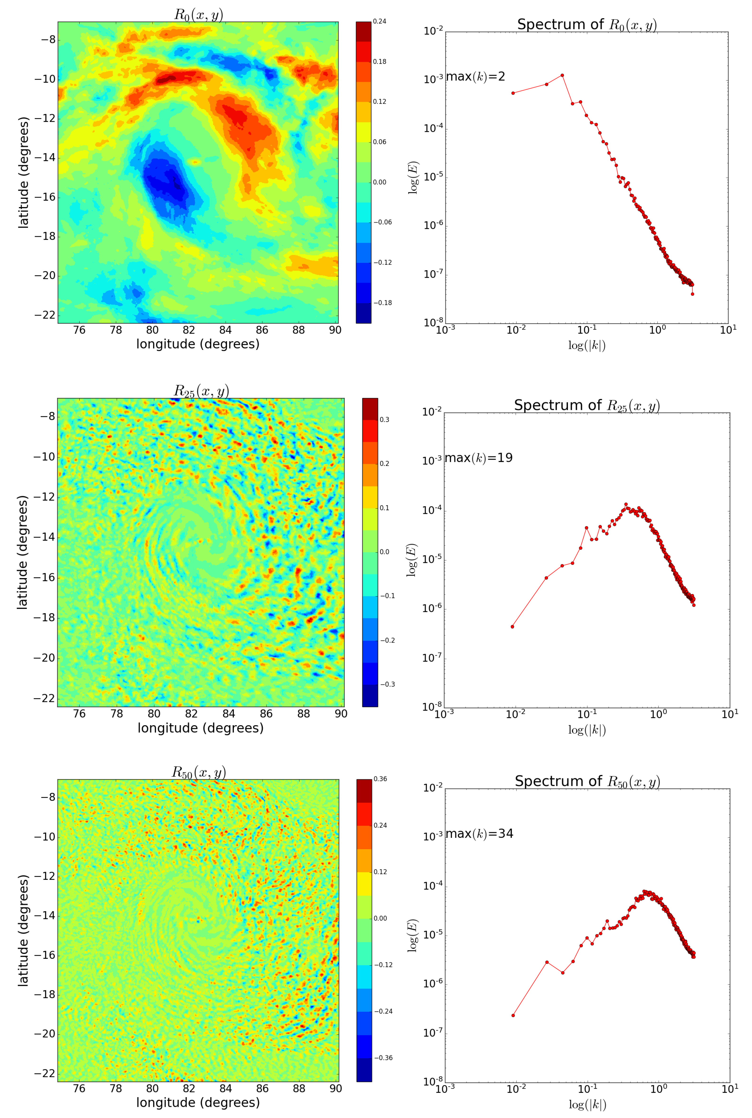
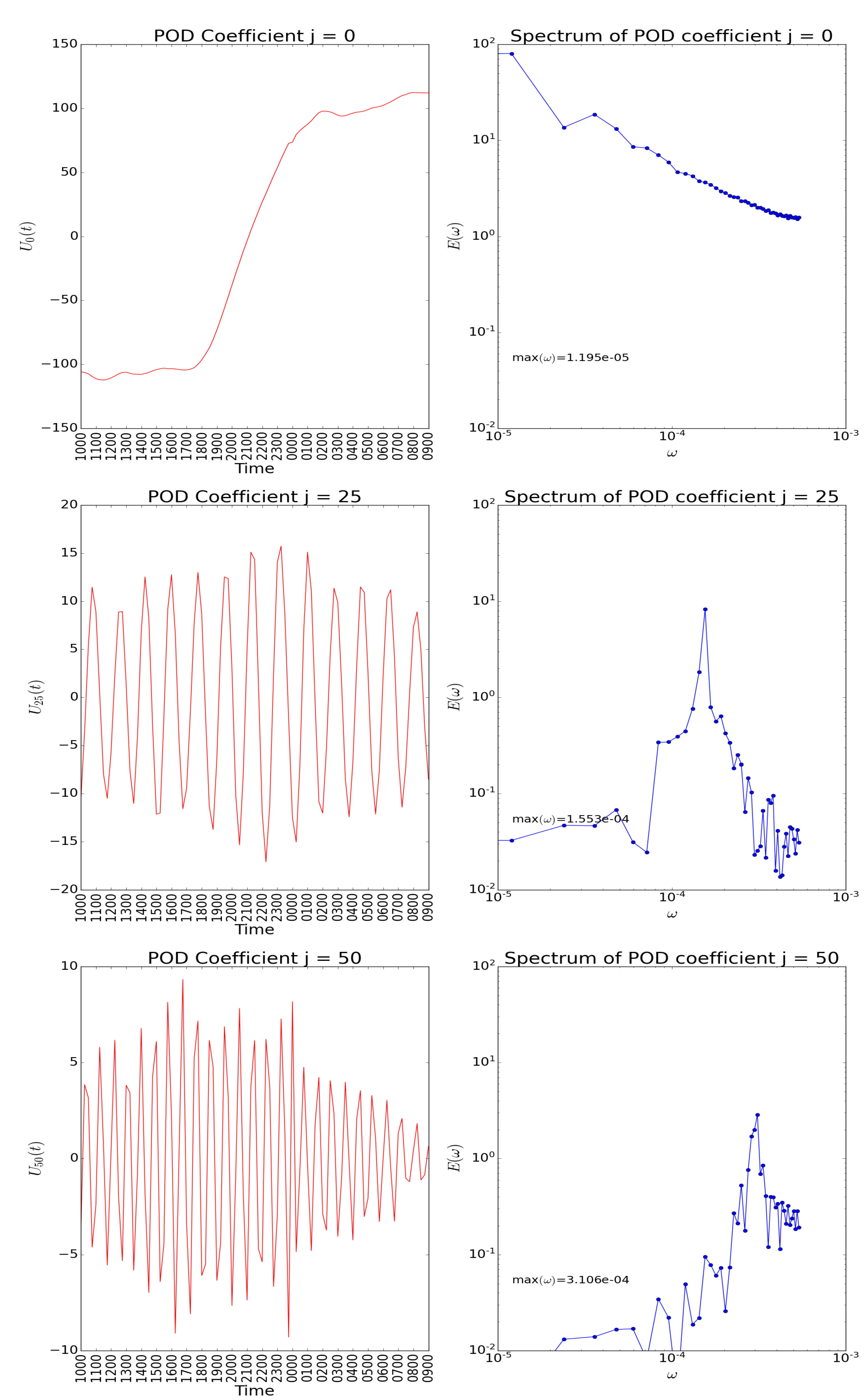
The three-scale separation hypothesis was further confirmed by constructing the spectra, shell-integrated in the Fourier space, corresponding to each of the POD eigenfunctions. In Figure 4, we show the example of three eigenfunctions, corresponding to $j=0$, $j=25$, $j=50$, which we associate to the macro-, meso- and small-scales, respectively, for the Faraji cyclone. On the left panels, we show the contour plots of the eigenfunctions as a function of longitude and latitude, while on the right panels, we show the shell-integrated spectra of the three eigenfunctions. It is clear that, with increasing j (from top to bottom), the characteristic scales become smaller. This is also visible from the spectra shown in the right panels, in which the peaks corresponding to the typical length scales are clearly visible and they shift continuously towards higher wavenumbers, that is, smaller scales, as j increases.

In Figure 4, we print the maximum value of $\left|k\right|$, namely the wave vector of the peak of the spectra, which identifies the characteristic length scale ℓ of the eigenfunction ($k=2\pi /\ell$), normalized to the total dimension of the image ${\ell }_0=N_{\mathrm{lon}}\times \sqrt{A}=N_{\mathrm{lat}}\times \sqrt{A}=350\mathrm{pixels}\times \left(1\frac{\mathrm{Km}}{\mathrm{pixels}}\right)$. Although the peaks are rather well visible in the spectra, they do not correspond to a real delta function, which is a single plane wave in Fourier space. This happens essentially for several effects: (1) the data (as, consequently, the eigenfunctions) are not periodic; therefore, some spurious energy is found at the smaller scales (higher wave vectors) due to this effect; (2) we compute a discrete Fourier transform, that is, when the energy is not exactly concentrated on a single wave vector k, which corresponds to a integer multiple of the fundamental wavelength $k_0$, the energy itself is spread over the modes close to k; (3) as it is visible in the contour plots of the eigenfunctions, the structures observed may have different characteristic scales along the longitude and latitude directions, which can produce a broadening of the peaks when the spectra are shell-integrated over the two directions. Nevertheless, we observed that the trend corresponding to a continuous shift of the peaks of the spectra towards smaller characteristic length scales is present for all values of the POD eigenfunction order j.

Afterwards, we carried out the same kind of analysis on the temporal component of the POD spectrum, namely, we computed energy spectra for the temporal evolution of the j-th POD coefficient $U_j\left(t\right)$, by Fourier-transforming in time the function $U_j\left(t\right)$ for all the values of j. As done for the spatial analysis, we plotted the time evolution of the POD coefficients $U_0\left(t\right)$, $U_{25}\left(t\right)$ and $U_{50}\left(t\right)$, along with the corresponding spectra in Figure 5.

It is clearly visible from the plots in the left panels that the number of oscillations in time increases for increasing values of j, meaning that higher js correspond to higher frequencies of the POD coefficients. This is even visible in a more clear way by looking at the spectra of the coefficients, plotted on the right panels. Again, the spectra exhibit rather well defined peaks, which move towards higher frequencies with increasing values of j. We also notice that the peak does not correspond to a delta-like function. Once again, this may depend on the fact that the time behavior of the coefficients (as visible in the left part of the figure) is not really periodic, and that the true frequencies are not necessarily integer multiples of the fundamental frequency ${\omega }_0=2\pi /P$, P being the total observation period, given by: $P=N·\Delta t=93·15$ min.

As seen in Figure 5, we found that there was a monotonic shift towards the highest frequencies in the maximum values of the temporal spectra of the POD coefficients with increasing values of their order j. We therefore identified for each value of j the peak in the frequency spectra and plotted its value against j (not shown here), and we found that there is a linear relation between the two quantities, as already found for the spatial scales in the Fourier spectra in $\left|k\right|$. Therefore, we can easily associate, through a linear best-fit procedure, a value of frequency to each POD mode with index j, in analogy with what we did for the length scales. Starting from this result, in order to better characterize how the energy of the field is distributed as a function of the frequency, we evaluated the average energy spectrum of the POD coefficients for the temperature field, inferred from the remote sensing analysis, of the Faraji cyclone, and we plotted it in Figure 6, on a double logarithmic scale, as a function of the frequency $\omega$. In the plot, we calculated the energy as the eigenvalue ${\lambda }_j$, since this quantity represents the energy on the j-th mode averaged in time. The frequency, instead, is computed from the peaks of the Fourier spectra of each POD coefficient $U_j\left(t\right)$ inferred through the best-fit procedure explained above.

From the plot, it is clearly visible that, also in this case, we can distinguish three different zones, each one approximately described by a power law with different scalings, which correspond approximately to the same POD modes observed in the spatial spectra, confirming that a linear correspondence between spatial scales, temporal scales, and POD order of the eigenvalues/eigenfunctions exists. Therefore, we can assume that, in the frequency domain, the subdivision we made for the spatial scales in macro-, meso-, and small-scales, may hold. However, in the case of the frequency spectrum, the differences among the three zones are not so evident as in the cases of the spatial scales. The slopes of the power laws of the energy E as a function of the distribution of the frequencies $\omega$ are all quite close to −2, which means that the energy content decays continuously, as $\sim \frac{1}{{\omega }^2}$ for all three characteristic scales. The characteristic time scale t corresponding to the macro-, meso-, and small-scales are, respectively: $t\gtrsim 10$ h, $10\mathrm{h}\gtrsim t\gtrsim 3\mathrm{h}$ and $t\lesssim 3$ h.

The determination of the slopes in the frequency spectrum obtained through the POD coefficients and the separation among the three zones were carried out in the same way as we already did in Figure 3 for the averaged spectrum of temperature as a function of the spatial scales.

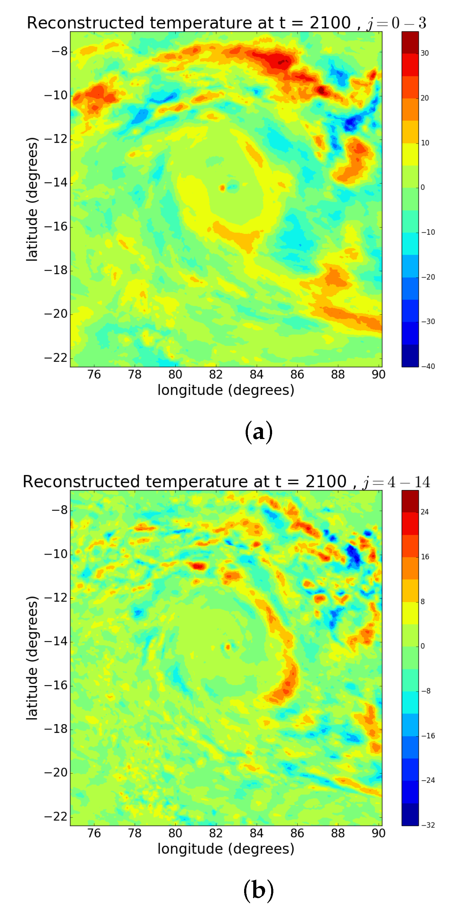
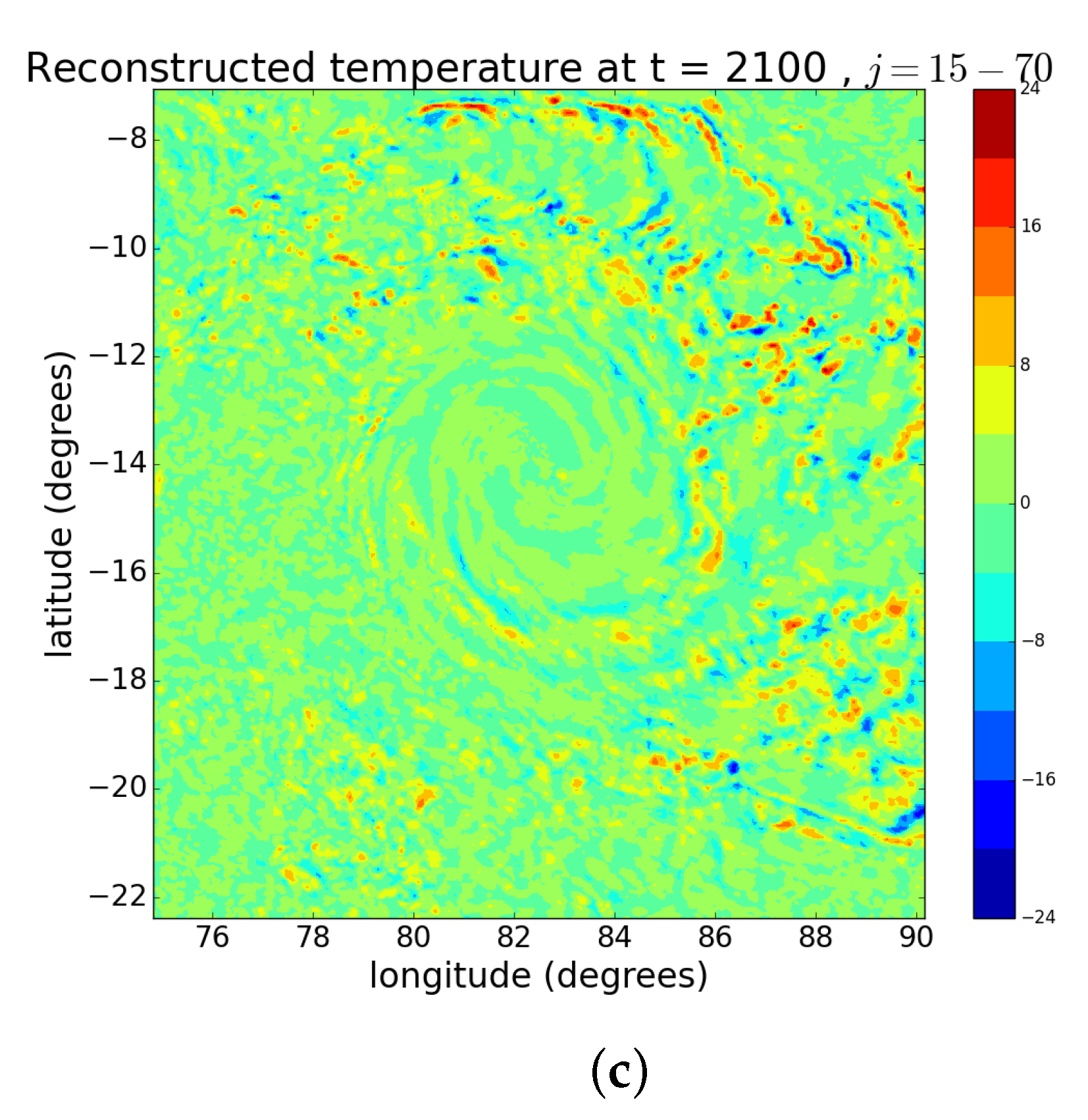
Finally, exploiting the linearity of the POD development, we can use Equation (6) to reconstruct the partial sums of the POD modes at different times for values of j in the macro-, meso-, and small-scales, to study how the turbulence evolves in the three different ranges of scales. The basic idea of this approach is that the turbulent evolution in the three zones is likely due to different mechanisms, operating at different length scales. We show examples of such reconstructions in Figure 7, which represents the spatial structures in the three different zones corresponding to the macroscales (panel a), the mesoscales (panel b), and the small-scales (panel c), for the data at 21.00 UTC on 8 February 2021.

From the reconstructions, the scale separation makes it possible to distinguish the differences in the internal structure of the cyclone and follow the evolution in time. With the large scales (panel a), we can identify the macroscale structures of the cyclone, while in the mesoscale (panel b), some filament structures remain, all rotating around the eye of the cyclone and with a tendency to expand towards the upper-right part of the cyclone. Some traces of those filament structures persist at smaller scales (panel c). However, here, the most evident phenomenon is the presence of small-scale spots, mainly spread in the zone of the cyclone external to the eye.

4. Discussion

In this work, we showed that, using data acquired from satellite missions, with the help of specific observational, acquisition, and processing procedures, it is possible to obtain significant results to understand the turbulence in extreme cyclonic phenomena. In particular, by exploiting remote sensing techniques, we captured a certain number of snapshots that were present in a given region of the globe at specific time instants, assigning temperature values to the pixels making up the reference matrix, from which it was possible to acquire a large amount of information on the physical nature of the phenomenon.

Specifically, the use of images acquired by sensors on geostationary satellites, such as SEVIRI, made it possible to apply a cyclone analysis from a purely dynamic point of view to an observational scalar field, such as the brightness temperature. We point out that, in this kind of investigation, the information along the line-of-sight is integrated, yielding a two-dimensional dataset at different sensing times. We used the POD technique, an analysis widely employed to study turbulent regimes in fluids, to extract useful information about the most energetic structures present in the evolution of the temperature field inside the Faraji hurricane, a category 5 cyclone on the Saffir–Simpson scale.

This technique makes it possible to separate the spatial and temporal behaviors in the evolution of the temperature field of the cyclone, starting from temperature variations, and to understand how these can influence the energy distributions at different scales. By extracting the POD eigenfunctions and coefficients through a suitably written numerical code, we found a correspondence between spatial scales and temporal scales in the POD modes. In particular, we found that, when increasing the order of the POD eigenfunction, both the typical length and time scales of the structures became smaller. From the differences in the slopes of the Fourier spectra in both the wave vector and frequency domains, it was possible to infer the presence of three different zones, which we called macro-, meso-, and small-scales, characterized by power laws with different spectral slopes. However, the differences in the slopes were much more evident for the spectra in the wave vector space than in the frequency domain, where, instead, the scaling of the energy was approximately proportional to ${\omega }^{-2}$.

There was another important observation concerning the reconstruction of the temperature field at the three different length scales—the macro-, meso-, and small-scales were mainly localized at different positions in the cyclone, which shows that their evolution was likely due to different dynamical mechanisms.

Different spectral slopes are commonly observed in the atmosphere. We cite, among others, the recent articles by Larsén et al. (2016) [21], Nosov et al. (2019) [22], and Shikhovtsev et al. (2019, 2021) [23,24]. However, a direct comparison of our results with the ones obtained in those papers was not easy to carry out because of the different conditions in the methods applied. In our case, we obtained the spectra of the temperature field in a hurricane, which is a highly nonstationary phenomenon, whilst those studies were related to measures of wind speed in standard atmospheric conditions. Moreover, they performed direct measurements of such quantities, whilst we obtain the temperature fields as indirect measures from the remote sensing analysis. Finally, our spectra were obtained by using the POD analysis, which is quite different from the standard Fourier analysis from which the spectra were obtained in those articles. However, a comparison of our work with the results of those articles can be very interesting and deserves a dedicated investigation.

Although this preliminary study supplies important information about the possibility of understanding, in more detail, the origin and evolution of a cyclone, drawing definitive conclusions concerning the latter point requires more extensive studies. First, the same analysis should be repeated on several different cyclones, with the aim of understanding whether the features found in the case of the Faraji hurricane are specific to this particular cyclone, or it is possible to extend this dynamical behavior to other cyclones of the same category, or of different categories, on the Saffir–Simpson scale. Moreover, it would be necessary to follow the time evolution of the structures in the three different zones of the cyclone to understand whether it is possible to understand the origins of the different dynamical behaviors that seem to characterize them. All of those studies will be the subjects of forthcoming papers.