
Compound Risk of Air Pollution and Heat Days and the Influence of Wildfire by SES across California, 2018–2020: Implications for Environmental Justice in the Context of Climate Change

Abstract
:1. Introduction
2. Data and Methods
2.1. Demographic Data
2.2. Temperature Data
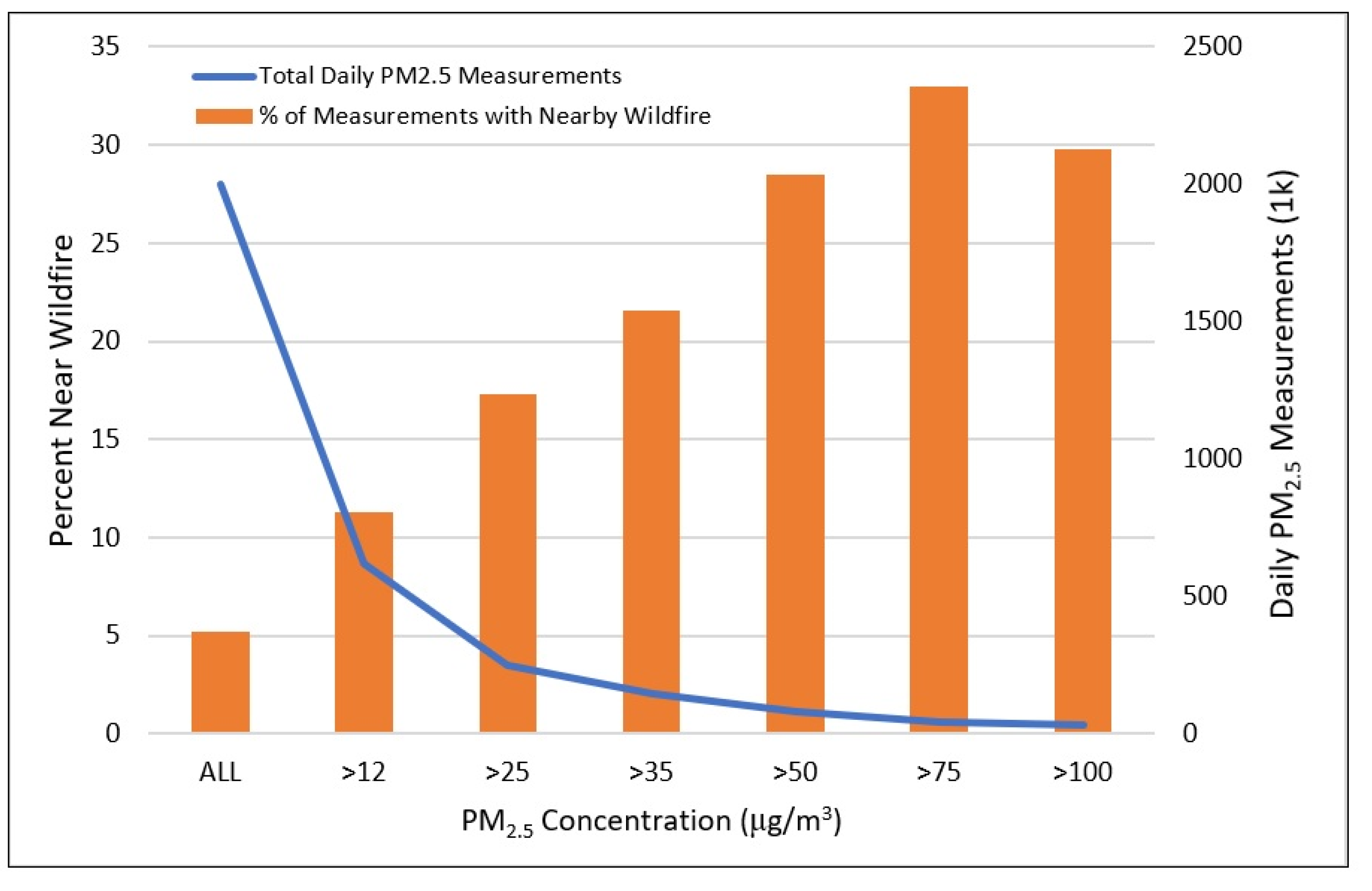
2.3. PM2.5 Data
- Remove malfunctioning sensor data based on a low frequency of change (5-day moving standard deviation of zero) in their reported measurements over time.
- Set PM2.5 outliers that exceed the sensor’s effective measurement range (daily values > 500 μg/m3) to 500 μg/m3.
- Identify periods of prolonged interruption or data loss due to power outages or data communication loss using a 75% completeness criterion (≥108 10 min measurements in a day).
- Examine the correlation from dual-channel readings for each sensor within a given month of operation based on calculated statistical anomality detection indicators as the coefficient of determination R2 > 0.8 and mean absolute error < 5.
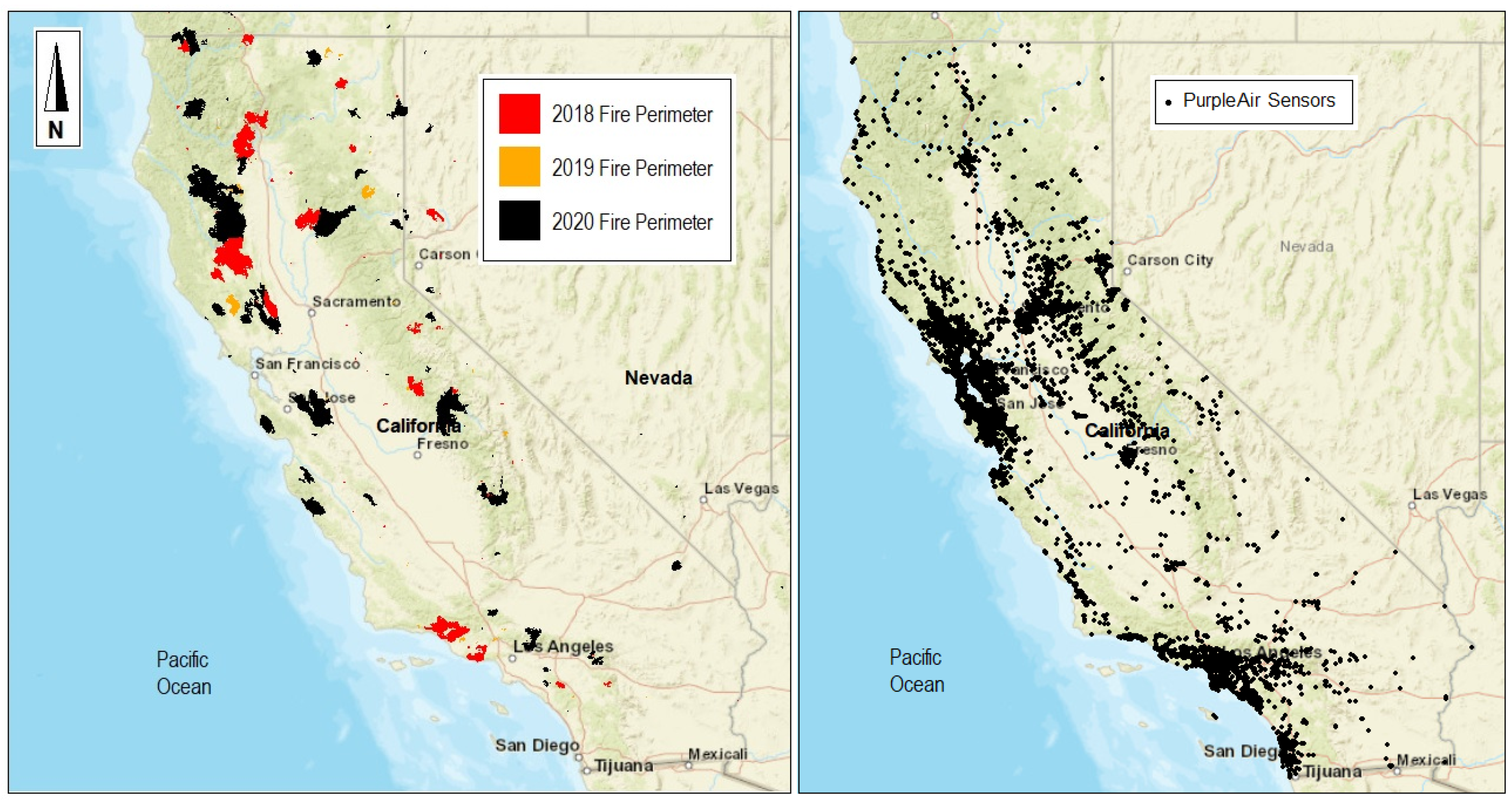
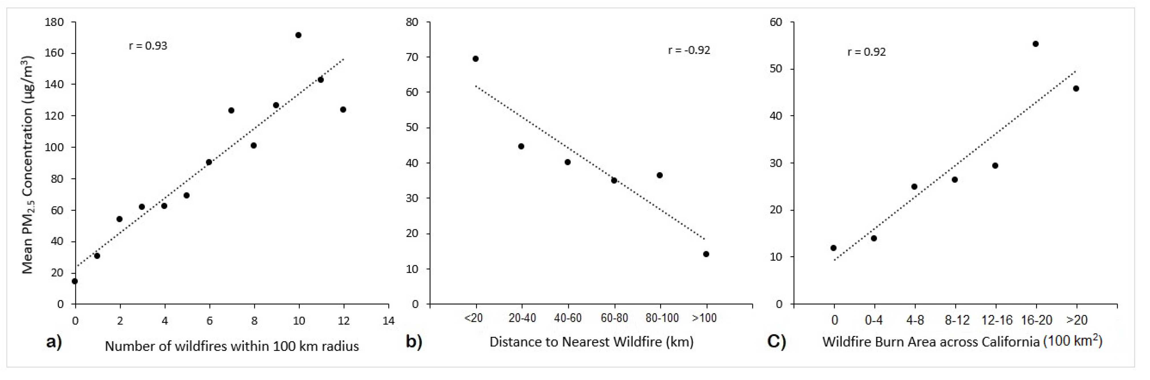
2.4. Wildfire Data
2.5. Regression Analysis
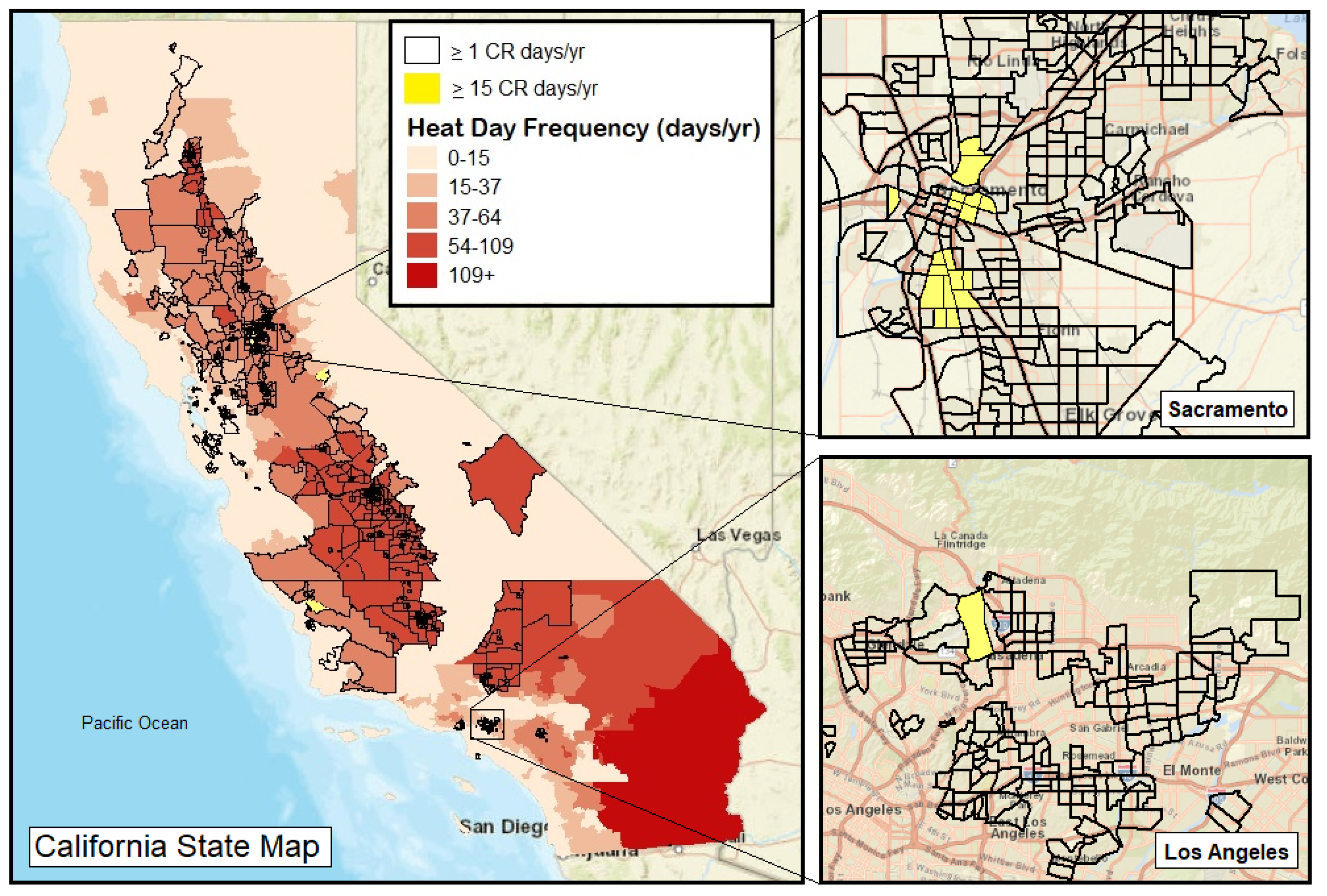
2.6. Census Tract Analysis
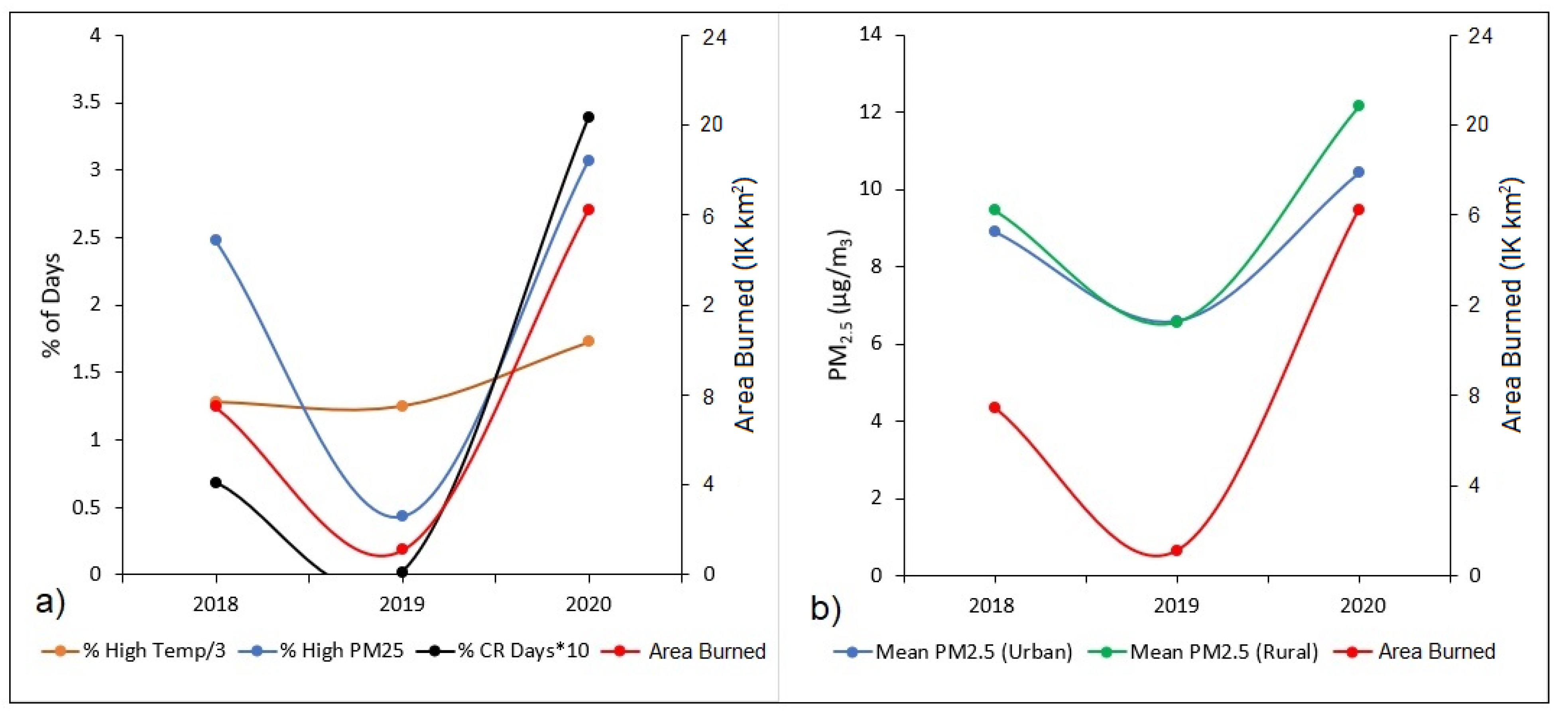
3. Results
4. Discussion
4.1. Census Tract Analysis
4.2. Strengths and Limitations
5. Conclusion
Supplementary Materials
Author Contributions
Funding
Data Availability Statement
Conflicts of Interest
References
- MassonDelmotte, V.; Zhai, A.P.; Pirani, S.L.; Connors, C.; Péan, S.; Berger, N.; Caud, Y.; Chen, L.; Goldfarb, M.I.; Gomis, M.; et al. IPCC, 2021: Summary for Policymakers. In Climate Change 2021: The Physical Science Basis. Contribution of Working Group I to the Sixth Assessment Report of the Intergovernmental Panel on Climate Change; Cambridge University Press: Cambridge, UK, 2021. [Google Scholar]
- Kent, S.T.; McClure, L.A.; Zaitchik, B.F.; Smith, T.T.; Gohlke, J.M. Heat waves and health outcomes in Alabama (USA): The importance of heat wave definition. Environ. Health Perspect. 2014, 122, 151–159. [Google Scholar] [CrossRef] [PubMed]
- Abasilim, C.; Friedman, L.S. Comparison of health outcomes from heat—related injuries by National Weather Service reported heat wave days and non—heat wave days—Illinois, 2013–2019. Int. J. Biometeorol. 2022, 66, 641–645. [Google Scholar] [CrossRef] [PubMed]
- Moghadamnia, M.T.; Ardalan, A.; Mesdaghinia, A.; Keshtkar, A.; Naddafi, K.; Yekaninejad, M.S. Ambient temperature and cardiovascular mortality: A systematic review and meta-analysis. PeerJ 2017, 2017, 3574. [Google Scholar] [CrossRef] [PubMed]
- Gasparrini, A.; Armstrong, B. The impact of heat waves on mortality. Epidemiology 2011, 22, 68–73. [Google Scholar] [CrossRef] [PubMed] [Green Version]
- Thompson, R.; Hornigold, R.; Page, L.; Waite, T. Associations between high ambient temperatures and heat waves with mental health outcomes: A systematic review. Public Health 2018, 161, 171–191. [Google Scholar] [CrossRef]
- Hansen, A.; Bi, P.; Nitschke, M.; Ryan, P.; Pisaniello, D.; Tucker, G. The effect of heat waves on mental health in a temperate Australian City. Environ. Health Perspect. 2008, 116, 1369–1375. [Google Scholar] [CrossRef] [Green Version]
- Baccini, M.; Biggeri, A.; Accetta, G.; Kosatsky, T.; Katsouyanni, K.; Analitis, A.; Anderson, H.R.; Bisanti, L.; D’Iippoliti, D.; Danova, J.; et al. Heat effects on mortality in 15 European cities. Epidemiology 2008, 19, 711–719. [Google Scholar] [CrossRef]
- Anderson, B.G.; Bell, M.L. How Heat, Cold, and Heat Waves Affect Mortality in the United States. Epidemiolog 2014, 23, 1–7. [Google Scholar] [CrossRef]
- Brooke Anderson, G.; Bell, M.L. Heat waves in the United States: Mortality risk during heat waves and effect modification by heat wave characteristics in 43 U.S. communities. Environ. Health Perspect. 2011, 119, 210–218. [Google Scholar] [CrossRef] [Green Version]
- NOAA Climate at a Glance. Available online: https://www.ncdc.noaa.gov/cag/statewide/time-series/ (accessed on 6 July 2022).
- Hulley, G.C.; Dousset, B.; Kahn, B.H. Rising Trends in Heatwave Metrics Across Southern California. Earth’s Futur. 2020, 8, e2020EF001480. [Google Scholar] [CrossRef]
- Smith, A.B. 2010–2019: A Landmark Decade of U.S. Billion-Dollar Weather and Climate Disasters. Available online: https://www.climate.gov/news-features/blogs/beyond-data/2010-2019-landmark-decade-us-billion-dollar-weather-and-climate (accessed on 6 July 2022).
- NOAA. U.S. Billion-Dollar Weather & Climate Disasters 1980–2020; Washington, DC, USA. 2020. Available online: https://www.ncei.noaa.gov/access/billions/ (accessed on 6 July 2022).
- DIttrich, R.; McCallum, S. How to measure the economic health cost of wildfires-A systematic review of the literature for northern America. Int. J. Wildl. Fire 2020, 29, 961–973. [Google Scholar] [CrossRef]
- CAL FIRE. Community Wildfire Prevention & Mitigation Report. 2019. Available online: https://bof.fire.ca.gov/media/8828/full-7-july-2019-directors-report.pdf (accessed on 6 July 2022).
- Westerling, A.L.; Hidalgo, H.G.; Cayan, D.R.; Swetnam, T.W. Warming and earlier spring increase Western U.S. forest wildfire activity. Science 2006, 313, 940–943. [Google Scholar] [CrossRef] [PubMed] [Green Version]
- California Department of Forestry and Fire Protection. Top 20 Largest California Wildfires. 2020. Available online: https://www.fire.ca.gov/media/4jandlhh/top20_acres.pdf (accessed on 6 July 2022).
- Agee, J.; Lolley, M. Thinning and prescribed fire effects on fuels and potential fire behavior in an eastern cascades forest. Fire Col. 2006, 2, 3–19. [Google Scholar] [CrossRef]
- Masri, S.; Scaduto, E.; Jin, Y.; Wu, J. Disproportionate impacts of wildfires among elderly and low-income communities in california from 2000–2020. Int. J. Environ. Res. Public Health 2021, 18, 3921. [Google Scholar] [CrossRef] [PubMed]
- McDermott, B.M.; Lee, E.M. Posttraumatic Stress Disorder and GeneralPsychopathology in Children and Adolescents Following a Wildfire Disaster. Can. J. Psychiatry 2005, 50, 137–143. [Google Scholar] [CrossRef] [PubMed] [Green Version]
- Reid, C.E.; Brauer, M.; Johnston, F.H.; Jerrett, M.; Balmes, J.R.; Elliott, C.T. Critical review of health impacts of wildfire smoke exposure. Environ. Health Perspect. 2016, 124, 1334–1343. [Google Scholar] [CrossRef] [Green Version]
- Asfaw, H.W.; McGee, T.K.; Christianson, A.C. Indigenous Elders’ Experiences, Vulnerabilities and Coping during Hazard Evacuation: The Case of the 2011 Sandy Lake First Nation Wildfire Evacuation. Soc. Nat. Resour. 2020, 33, 1273–1291. [Google Scholar] [CrossRef]
- Chen, H.; Samet, J.M.; Bromberg, P.A.; Tong, H. Cardiovascular health impacts of wildfire smoke exposure. Part. Fibre Toxicol. 2021, 18, 2. [Google Scholar] [CrossRef]
- Gan, R.W.; Liu, J.; Ford, B.; O’Dell, K.; Vaidyanathan, A.; Wilson, A.; Volckens, J.; Pfister, G.; Fischer, E.V.; Pierce, J.R.; et al. The association between wildfire smoke exposure and asthma-specific medical care utilization in Oregon during the 2013 wildfire season. J. Expo. Sci. Environ. Epidemiol. 2020, 30, 618–628. [Google Scholar] [CrossRef]
- Wu, J.; Winer, A.; Delfino, R. Exposure assessment of particulate matter air pollution before, during, and after the 2003 Southern California wildfires. Atmos. Environ. 2006, 40, 3333–3348. [Google Scholar] [CrossRef] [Green Version]
- Vedal, S.; Dutton, S.J. Wildfire air pollution and daily mortality in a large urban area. Environ. Res. 2006, 102, 29–35. [Google Scholar] [CrossRef] [PubMed]
- Aguilera, R.; Gershunov, A.; Ilango, S.D.; Morales, J.G. Santa Ana Winds of Southern California Impact PM2.5 with and without Smoke from Wildfires. GeoHealth 2019, 4, e2019GH000225. [Google Scholar] [CrossRef] [Green Version]
- Cleland, S.E.; West, J.J.; Jia, Y.; Reid, S.; Raffuse, S.; Neill, S.O.; Serre, M.L. Estimating Wildfire Smoke Concentrations during the October 2017 California Fires through BME Space/Time Data Fusion of Observed, Modeled, and Satellite-Derived PM2.5. Environ. Sci. Technol. 2020, 54, 13439–13447. [Google Scholar] [CrossRef]
- Anenberg, S.C.; Haines, S.; Wang, E.; Nassikas, N.; Kinney, P.L. Synergistic health effects of air pollution, temperature, and pollen exposure: A systematic review of epidemiological evidence. Environ. Health A Glob. Access Sci. Source 2020, 19, 130. [Google Scholar] [CrossRef] [PubMed]
- Prashant, K.; Morawska, L.; Martani, C.; Biskos, G.; Neophytou, M.; Di Sabatino, S.; Bell, M.; Norford, L.; Britter, R. The rise of low-cost sensing for managing air pollution in cities. Environ. Int. 2015, 75, 199–205. [Google Scholar]
- Bi, J.; Stowell, J.; Seto, E.Y.W.; English, P.B.; Al-Hamdan, M.Z.; Kinney, P.L.; Freedman, F.R.; Liu, Y. Contribution of low-cost sensor measurements to the prediction of PM2.5levels, A case study in Imperial County, California, USA. Environ. Res. 2020, 180, 108810. [Google Scholar] [CrossRef] [PubMed]
- Morawska, L.P.K.; Thai, X.; Liu, A.; Asumadu-Sakyi, G.; Ayoko, A.; Bartonova, A.; Bedini, F.; Chai, B.; Christensen, M.; Dunbabin, J.; et al. Applications of low-cost sensing technologies for air quality monitoring and exposure assessment: How far have they gone? Environ. Int. 2018, 116, 286–299. [Google Scholar] [CrossRef]
- Pope, F.D.; Gatari, M.; Ng’ang’a, D.; Poynter, A.; Blake, R. Airborne particulate matter monitoring in Kenya using calibrated low-cost sensors. Atmos. Chem. Phys. 2018, 18, 15403–15418. [Google Scholar] [CrossRef] [Green Version]
- Bi, J.; Wildani, A.; Chang, H.H.; Liu, Y. Incorporating Low-Cost Sensor Measurements into High-Resolution PM2.5 Modeling at a Large Spatial Scale. Environ. Sci. Technol. 2020, 54, 2152–2162. [Google Scholar] [CrossRef]
- Delp, W.W.; Singer, B.C. Wildfire Smoke Adjustment Factors for Low-Cost and Professional PM 2.5 Monitors with Optical Sensors. Sensors 2020, 20, 3683. [Google Scholar] [CrossRef]
- Finlayson-Pitts, B.J.; James, N.; Pitts, J. Chemistry of the Upper and Lower Atmosphere: Theory, Experiments, and Applications; Academic Press: London, UK, 2000. [Google Scholar]
- Agyapong, V.I.O.; Ritchie, A.; Brown, M.R.G.; Noble, S.; Mankowsi, M.; Denga, E.; Nwaka, B.; Akinjise, I.; Corbett, S.E.; Moosavi, S.; et al. Long-Term Mental Health Effects of a Devastating Wild fire Are Amplified by Socio-Demographic and Clinical Antecedents in Elementary and High School Staff. Front. Psychiatry 2020, 11, 448. [Google Scholar] [CrossRef] [PubMed]
- Mikati, I.; Benson, A.F.; Luben, T.J.; Sacks, J.D.; Richmond-Bryant, J. Disparities in distribution of particulate matter emission sources by race and poverty status. Am. J. Public Health 2018, 108, 480–485. [Google Scholar] [CrossRef] [PubMed]
- Morello-Frosch, R.; Pastor, M.; Porras, C.; Sadd, J. Environmental justice and regional inequality in Southern California: Implications for furture research. Environ. Health Perspect. 2002, 110, 149–154. [Google Scholar] [CrossRef] [PubMed] [Green Version]
- Chakraborty, J.; Zandbergen, P.A. Children at risk: Measuring racial/ethnic disparities in potential exposure to air pollution at school and home. J. Epidemiol. Community Health 2007, 61, 1074–1079. [Google Scholar] [CrossRef] [Green Version]
- Gaffron, P.; Niemeier, D. School locations and traffic Emissions—Environmental (In)justice findings using a new screening method. Int. J. Environ. Res. Public Health 2015, 12, 2009–2025. [Google Scholar] [CrossRef] [Green Version]
- Mirabelli, M.C.; Wing, S.; Marshall, S.W.; Wilcosky, T.C. Race, poverty, and potential exposure of middle-school students to air emissions from confined swine feeding operations. Environ. Health Perspect. 2006, 114, 591–596. [Google Scholar] [CrossRef] [Green Version]
- Pastor, M.; Sadd, J.L.; Morello-Frosch, R. Who’s minding the kids? Pollution, public schools, and environmental justice in Los Angeles. Soc. Sci. Q. 2002, 83, 263–280. [Google Scholar] [CrossRef]
- United Church of Christ Commission for Racial Justice Toxic Waste and Race in he United States: A National Report on the Racial and Socio-Economic Characterist!cs of Communities with Hazardous Waste Sites; United Church of Christ: New York, NY, USA, 1987.
- Xu, R.; Zhao, Q.; Coelho, M.S.Z.S.; Salvida, P.H.N.; Abramson, M.J.; Li, S.; Guo, Y. Socioeconomic inequality in vulnerability to all-cause and cause-specific hospitalisation associated with temperature variability: A time-series study in 1814 Brazilian cities. Lancet 2020, 4, 566–676. [Google Scholar] [CrossRef]
- Son, J.-Y.; Choi, H.M.; Miranda, M.L.; Bell, M.L. Exposure to heat during pregnancy and preterm birth in North Carolina_ Main effect and disparities by residential greenness, urbanicity, and socioeconomic status. Environ. Res. 2021, 204, 112315. [Google Scholar] [CrossRef]
- University of California Merced The Climatology Lab. Available online: https://www.climatologylab.org/ (accessed on 12 June 2021).
- Abatzoglou, J.T. Development of gridded surface meteorological data for ecological applications and modelling. Int. J. Climatol. 2013, 33, 121–131. [Google Scholar] [CrossRef]
- PurpleAir Inc. PurpleAir. Available online: https://www2.purpleair.com/ (accessed on 10 December 2021).
- Ardon-Dryer, K.; Dryer, Y.; Williams, J.N.; Moghimi, N. Measurements of PM2.5 with PurpleAir under atmospheric conditions. Atmos. Meas. Tech. 2020, 13, 5441–5458. [Google Scholar] [CrossRef]
- Mousavi, A.; Wu, J. Indoor-Generated PM2.5 during COVID-19 Shutdowns across California: Application of the PurpleAir Indoor-Outdoor Low-Cost Sensor Network. Environ. Sci. Technol. 2021, 55, 5648–5656. [Google Scholar] [CrossRef] [PubMed]
- Lu, Y.; Giuliano, G.; Habre, R. Estimating hourly PM2.5 concentrations at the neighborhood scale using a low-cost air sensor network: A Los Angeles case study. Environ. Res. 2021, 195, 110653. [Google Scholar] [CrossRef]
- USDA. National Infrared Operations/NIROPS Hi-Tech Heat-Seekers. 2017. Available online: https://fsapps.nwcg.gov/nirops/pages/about (accessed on 6 July 2022).
- SAS Institute Inc. SAS® 9.4 Statements: Reference, 3rd ed.; SAS Institute Inc.: Cary, NC, USA, 2014. [Google Scholar]
- Belsley, D.A.; Kuh, E.; Welsch, R.E. Regression Diagnostics: Identifying Influential Data and Sources of Collinearity; John Wiley & Sons: New York, NY, USA, 1980. [Google Scholar]
- SAS Institute Inc. The Reg Procedure. Collinearity Diagnostics. Available online: https://documentation.sas.com/doc/en/statcdc/14.2/statug/statug_reg_details24.htm (accessed on 6 July 2022).
- Tan, J.; Zheng, Y.; Tang, X.; Guo, C.; Li, L.; Song, G.; Zhen, X.; Yuan, D.; Kalkstein, A.J.; Li, F.; et al. The urban heat island and its impact on heat waves and human health in Shanghai. Int. J. Biometeorol. 2010, 54, 75–84. [Google Scholar] [CrossRef]
- USEPA. The National Ambient Air Quality Standards for Particle Matter: Revised Air Quality Standards for Particle Pollution and Updates to the Air Quality Index (AQI); Washington, DC, USA. 2012. Available online: https://www.epa.gov/sites/default/files/2016-04/documents/2012_aqi_factsheet.pdf (accessed on 6 July 2022).
- Dewees, S.; Marks, B. Twice invisible: Understanding Rural Native America. First Nations Dev. Inst. 2017, 1–10. Available online: https://www.usetinc.org/wp-content/uploads/bvenuti/WWS/2017/May%202017/May%208/Twice%20Invisible%20-%20Research%20Note.pdf (accessed on 6 July 2022).
- Rodríguez, H.; Quarantelli, E.L.; Dynes, R.R. Handbook of Disaster Research; 2007; ISBN 9783319632537. Available online: https://link.springer.com/book/10.1007/978-0-387-32353-4 (accessed on 6 July 2022).
- American Lung Association Children and Air Pollution. Available online: https://www.lung.org/clean-air/outdoors/who-is-at-risk/children-and-air-pollution (accessed on 2 July 2022).
- Liu, J.C.; Mickley, L.J.; Sulprizio, M.P.; Dominici, F.; Yue, X.; Ebisu, K.; Anderson, G.B.; Khan, R.F.A.; Bravo, M.A.; Bell, M.L. Particulate air pollution from wildfires in the Western US under climate change. Clim. Change 2016, 138, 655–666. [Google Scholar] [CrossRef] [PubMed] [Green Version]
- Enayati Ahangar, F.; Pakbin, P.; Hasheminassab, S.; Epstein, S.A.; Li, X.; Polidori, A.; Low, J. Long-term trends of PM2.5 and its carbon content in the South Coast Air Basin: A focus on the impact of wildfires. Atmos. Environ. 2021, 255, 118431. [Google Scholar] [CrossRef]
- McClure, C.D.; Jaffe, D.A. US particulate matter air quality improves except in wildfire-prone areas. Proc. Natl. Acad. Sci. USA 2018, 115, 7901–7906. [Google Scholar] [CrossRef] [PubMed] [Green Version]
- O’Dell, K.; Ford, B.; Fischer, E.V.; Pierce, J.R. Contribution of Wildland-Fire Smoke to US PM 2.5 and Its Influence on Recent Trends. Environ. Sci. Technol. 2019, 53, 1797–1804. [Google Scholar] [CrossRef]
- Brown, K.; Mijic, A. Integrating green and blue spaces into our cities: Making it happen. Grantham Inst. 2020, 30, 1–10. [Google Scholar]
- Aram, F.; Garcia, E.H.; Solgi, E.; Mansournia, S. Urban green space cooling effect in cities. Heliyon 2019, 5, e01339. [Google Scholar] [CrossRef] [PubMed] [Green Version]
- Liu, W.; Zhao, H.; Sun, S.; Xu, X.; Huang, T.; Zhu, J. Green Space Cooling Effect and Contribution to Mitigate Heat Island Effect of Surrounding Communities in Beijing Metropolitan Area. Front. Public Health 2022, 10, 870403. [Google Scholar] [CrossRef] [PubMed]
- Sun, Y.; Mousavi, A.; Masri, S.; Wu, J. Socioeconomic Disparities of Low-Cost Air Quality Sensors in California, 2017–2020. Am. J. Public Health 2022, 112, 434–442. [Google Scholar] [CrossRef] [PubMed]


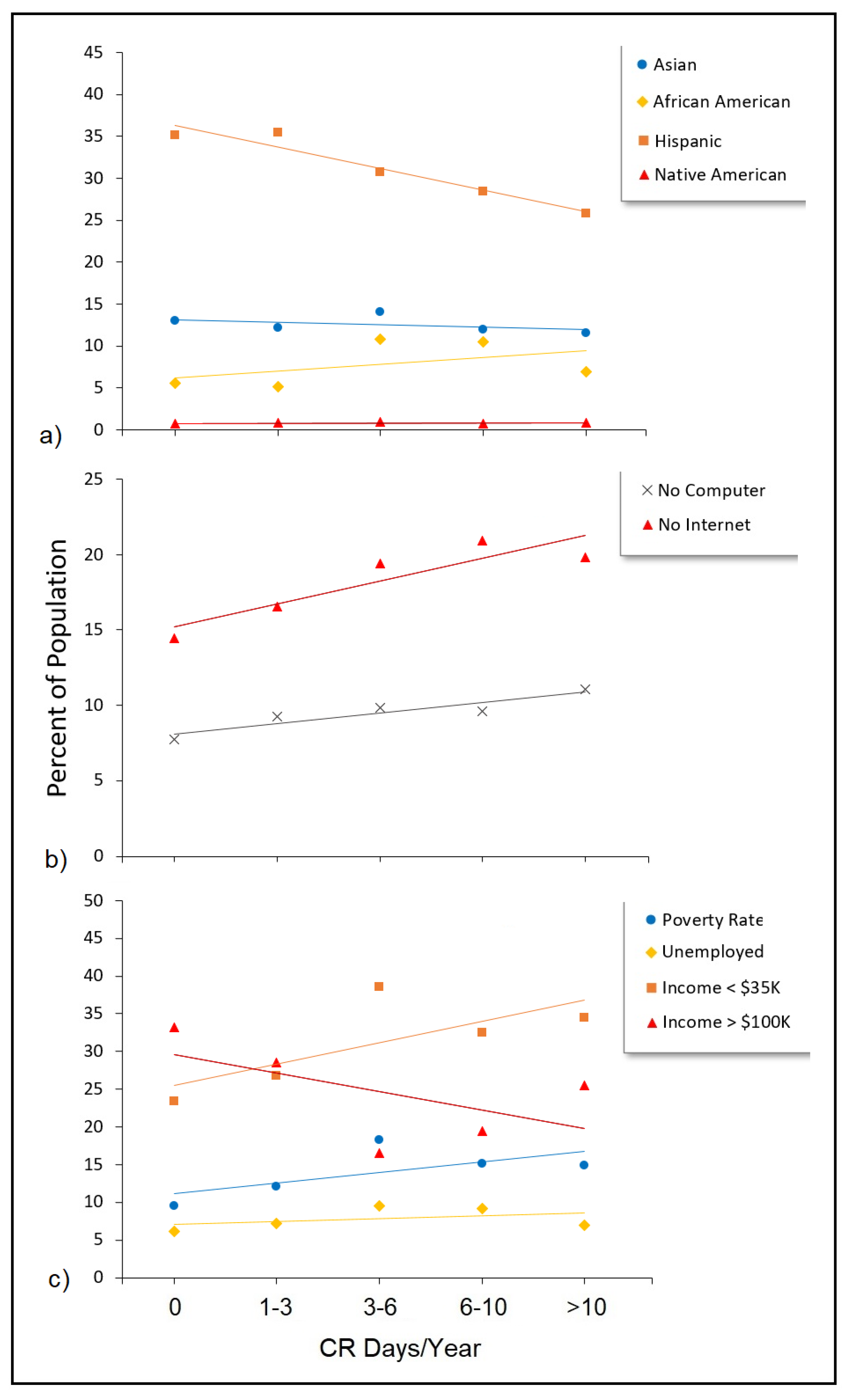
| Effect Estimate | p-Value | |
|---|---|---|
| Asian Residents (%) | −0.00474 | 0.0011 |
| African American Residents (%) | 0.00188 | 0.4584 |
| Hispanic Residents (%) | 0.00086 | 0.3099 |
| Native American Residents (%) | 0.02302 | 0.0147 |
| Households without Computer (%) | 0.03320 | <0.0001 |
| Households without Internet (%) | 0.02240 | <0.0001 |
| Poverty Rate (%) | 0.03108 | <0.0001 |
| Unemployed (%) | 0.05774 | <0.0001 |
| Income < $35K (%) | 0.02134 | <0.0001 |
| Income > $100K (%) | −0.01508 | <0.0001 |
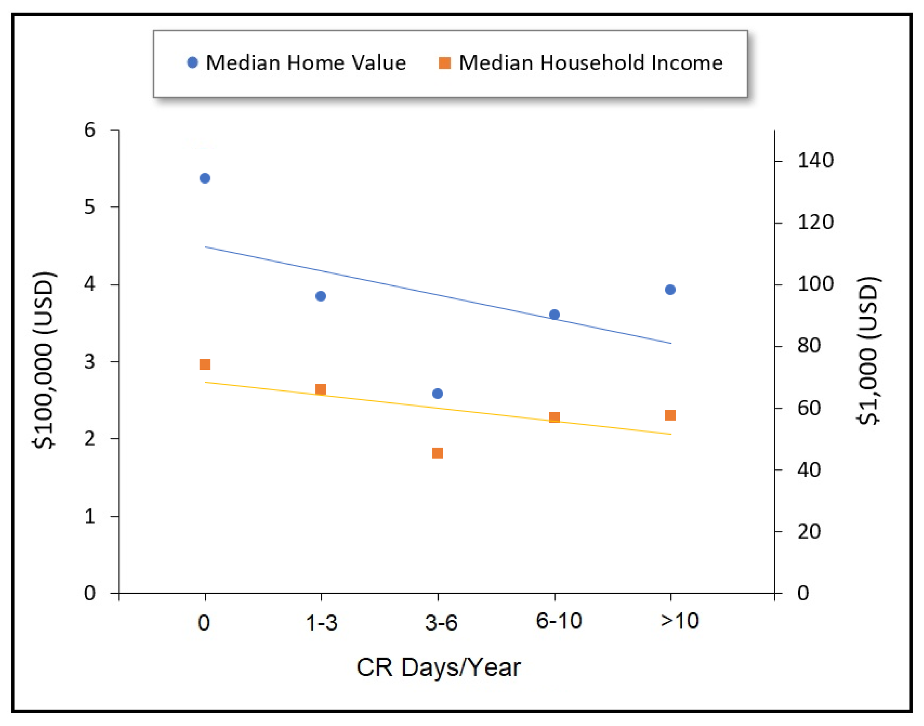
| Median Home Value ($100K) | −0.13890 | <0.0001 |
| Median Household Income ($10K) | −0.07261 | <0.0001 |
| Residents without College Degree (%) | 0.01157 | <0.0001 |
| Residents < Age 5 (%) | 0.00067 | <0.0001 |
| Residents > Age 65 (%) | −0.000091 | 0.1094 |
| Effect Estimate | p-Value | |
|---|---|---|
| Intercept | 0.45298 | <0.0001 |
| Hispanic Residents (%) | −0.01257 | <0.0001 |
| African American Residents (%) | -0.01265 | <0.0001 |
| Households without a Computer (%) | 0.02272 | <0.0005 |
| Unemployment Rate (%) | 0.03616 | <0.0001 |
| Poverty Rate (%) | 0.03265 | <0.0001 |
| Residents < Age 5 (%) | 0.00069 | <0.0001 |
| EE | p-Value | |
|---|---|---|
| Intercept | 49.49 | <0.001 |
| Distance to nearest wildfire (10 km) | −1.66 | <0.001 |
| Area of nearest wildfire (10 km2) | 0.14 | <0.001 |
| Area of all wildfires in California (10 km2) | 0.17 | <0.001 |
Publisher’s Note: MDPI stays neutral with regard to jurisdictional claims in published maps and institutional affiliations. |
© 2022 by the authors. Licensee MDPI, Basel, Switzerland. This article is an open access article distributed under the terms and conditions of the Creative Commons Attribution (CC BY) license (https://creativecommons.org/licenses/by/4.0/).
Share and Cite
Masri, S.; Jin, Y.; Wu, J. Compound Risk of Air Pollution and Heat Days and the Influence of Wildfire by SES across California, 2018–2020: Implications for Environmental Justice in the Context of Climate Change. Climate 2022, 10, 145. https://doi.org/10.3390/cli10100145
Masri S, Jin Y, Wu J. Compound Risk of Air Pollution and Heat Days and the Influence of Wildfire by SES across California, 2018–2020: Implications for Environmental Justice in the Context of Climate Change. Climate. 2022; 10(10):145. https://doi.org/10.3390/cli10100145
Chicago/Turabian StyleMasri, Shahir, Yufang Jin, and Jun Wu. 2022. "Compound Risk of Air Pollution and Heat Days and the Influence of Wildfire by SES across California, 2018–2020: Implications for Environmental Justice in the Context of Climate Change" Climate 10, no. 10: 145. https://doi.org/10.3390/cli10100145