On the Bayesian Mixture of Generalized Linear Models with Gamma-Distributed Responses

Abstract

This paper proposes enhanced studies on a model consisting of a finite mixture framework of generalized linear models (GLMs) with gamma-distributed responses estimated using the Bayesian approach coupled with the Markov Chain Monte Carlo (MCMC) method. The log-link function, which relates the mean and linear predictors of the model, is implemented to ensure non-negative values of the predicted gamma-distributed responses. The simulation-based inferential processes related to the Bayesian-MCMC method is carried out using the Gibbs sampler algorithm. The performance of proposed model is conducted through two real data applications on the gross domestic product per capita at purchasing power parity and the annual household income per capita. Graphical posterior predictive checks are carried out to verify the adequacy of the fitted model for the observed data. The predictive accuracy of this model is compared with other Bayesian models using the widely applicable information criterion (WAIC). We find that the Bayesian mixture of GLMs with gamma-distributed responses performs properly when the appropriate prior distributions are applied and has better predictive accuracy than the Bayesian mixture of linear regression model and the Bayesian gamma regression model.

1. Introduction

The finite mixture model, as a class of model-based clustering methods, provides a flexible model for capturing heterogeneous data in a data-driven manner. The finite mixture of statistical distribution, commonly called the finite mixture distribution, is the most basic type of finite mixture model. Due to its flexibility for modeling heterogeneous data, the finite mixture model with its various developments has been widely studied in the research. The finite mixture model of the exponential family of distributions is one of the models included in that study. Wiper et al. (2001) determined a mixture of gamma distribution for estimating some quantities for a M/G/1 queue. Lopera et al. (2011) introduced a Bayesian analysis for the mixture of normal-exponential distributions including joint modeling of the mean and variance. Garrido and Cepeda (2012) proposed the mixtures of normal and gamma distributions belonging to the biparametric exponential family. The simulated studies and applications of heteroscedastic Weibull-Normal mixture models with the Bayesian approach were discussed in Garrido and Cuervo (2014).

Further advanced models have been established by including generalized linear models (GLMs) in each mixture component. The finite mixture of GLMs allows the construction of different parameters in each mixture component, hence, it can accommodate different heterogeneous cases that occur in the data. Wedel and Kamakura (2000) defined this model as the Generalized Mixture Regression Models (GLIMMIX), whereas Grün and Leisch (2008) called it the Finite Mixtures of Generalized Linear Regression Models.

Inferential methods, through frequentist or Bayesian approaches, can be implemented to estimate the finite mixture of GLMs. The Bayesian framework, which performs an estimating procedure concerning the posterior distribution of parameters, has some advantages when used to determine the parameter of the finite mixture model. One of the advantages of the Bayesian approach is that when regularity conditions are not fulfilled, i.e., when sample size and mixture component proportions are small, the Bayesian parameter estimation still delivers a valid inference and does not need asymptotic normality (Frühwirth-Schnatter 2006). Since the joint posterior distribution incorporates all possible sample observations into the maximum number of mixture components, its determining process through the Bayesian framework is most difficult to solve analytically. A numerical approach, the well-known Markov Chain Monte Carlo (MCMC) method, needs to be implemented to deal with that problem. The Gibbs sampler algorithm carried out by augmenting the data is one of the algorithms in MCMC that is commonly applied to generate iteratively random samples from the posterior distribution of parameters. The iterative computing procedure conducted within the MCMC makes a structured simulation-based inference when the Bayesian framework is coupled with the MCMC.

Many papers studied the finite mixture of GLMs estimated by the Bayesian-MCMC approach. Lenk and DeSarbo (2000) introduced the finite mixture of GLMs with random effects and implemented the Gibbs sampler algorithm to fit the regression coefficients formed as a finite mixture of normal distributions. Hurn et al. (2003) developed a mixture of the Poisson and the logistic regression models, which were estimated through the Gibbs sampler and the Metropolis-Hastings algorithms. The application of a finite mixture of negative binomial regression for modeling heterogeneity in accident data was analyzed by Park and Lord (2009). Meanwhile, the mixture of Bernoulli regression was proposed by Iriawan et al. (2018) to determine the admission conditions of the Bidikmisi scholarship for students wanting to enroll in universities.

The purpose of this study is to examine more extensively a finite mixture of GLMs with gamma-distributed responses with a known number of mixture components estimated by using the Bayesian-MCMC approach. GLMs with gamma-distributed responses are commonly applied to model non-negative, continuous, and positive-skewed data, which are characteristics of economic distribution data. The study focuses on the application side rather than the theoretical side to find out the advantages of the proposed model. We consider appropriate descriptions of how Bayesian-MCMC is used to estimate the proposed model; then, we demonstrate the particular performances of the proposed model using two real applications with distinct response distributions. In the first real case, i.e., modeling the gross domestic product at purchasing power parity per capita, we study the responses that have a gamma distribution. In contrast, in the second real case, i.e., modeling the household income clustered in different sub-populations, we examine the responses that do not fit the gamma distribution but satisfy the essential characteristics required for developing the proposed model. Furthermore, specific extreme responses are detected in each mixture component in this second real case. Those two case studies are expected to strengthen the proposed model’s application. The performance of the proposed model in prediction accuracy is compared with the Bayesian mixture of linear regression and the Bayesian gamma regression model through the WAIC. The Bayesian-MCMC computations are performed using the BUGS language through MultiBUGS, a software that supports the parallel computation of MCMC chains (Goudie et al. 2020). The convergence diagnostic of MCMC chains is verified through a CODA package which was developed by Plummer et al. (2006).

This paper is arranged in the following steps: in Section 2, the flowchart diagram of the research methodology is described. In Section 3, the Bayesian framework for inferencing the finite mixture of GLMs with gamma-distributed responses is provided with the required computation schemes for the MCMC method. In addition to describe the WAIC, we also present the Gelman-Rubin method, which is considered to be a suitable method for assessing the convergent condition of MCMC chains. The real data applications are presented in Section 4; Section 5 provides some discussions; and the main conclusions are given in Section 6.

2. Materials and Methods

The workflow of the research methodology that is applied in this paper is presented in Figure 1.

3. Bayesian Approach for the Finite Mixture of GLMs

In a generalized linear model, a framework is constructed through a relationship between random samples $y_i$ as a response and a vector of predictors $x_i=(1,x_{i1},\dots ,x_{ip}{)}^t$ with $x_{ij}$ as a j-th predictor on the i-th observation, $j=1,2,\dots ,p$, and $i=1,2,\dots ,n$. The responses are considered to be generated from a family of exponential distributions. The structure of the GLMs is formulated as (1).

$${\eta }_i=g({\mu }_i)=g(E(y_i|x_i))=x_i^t\mathit{\beta }={\beta }_0+{\displaystyle \sum _{j=1}^p}{\beta }_j{x}_{ij}$$

(1)

where ${\eta }_i$ is a linear predictor; $g(.)$ is a link function; ${\mu }_i$ is an expected value of the response $y_i$; and $\mathit{\beta }$ is a vector of unknown coefficients; $\mathit{\beta }=({\beta }_0,{\beta }_1,\dots ,{\beta }_p{)}^t$. The vector $\mathit{\beta }$ can represent the unknown parameters that describe the relationship between predictor variables and the response.

Grün and Leisch (2008) developed a finite mixture of a generalized linear regression model by inserting the generalized linear model (1) into mixture components. A finite mixture of GLMs with K known mixture components is defined by (2):

$$h(y_i|x_i,\mathit{\vartheta })={\displaystyle \sum _{k=1}^K}{w}_k{f}_k(y_i|x_i,{\mathit{\theta }}_{\mathrm{k}})$$

(2)

where $\mathit{\vartheta }$ denotes a vector of all parameters included in the model; $f_k(y_i|x_i,{\mathit{\theta }}_{\mathrm{k}})$ represents the density function which is assumed to be a family of exponential distributions having a particular vector of parameter ${\mathit{\theta }}_{\mathrm{k}}$; and $w_k$ is a mixing parameter that satisfies ${\displaystyle {\sum }_{k=1}^K}{w}_k=1$ and $w_k>0$, $\forall k$, $k=1,2,\dots ,K$. Thus, the mean on the k-th mixture component is provided by (3):

$${\mu }_{ik}=g^{-1}(x_i^t{\mathit{\beta }}_k)$$

(3)

where ${\mathit{\beta }}_k=({\beta }_{0k},{\beta }_{1k},\dots {\beta }_{pk}{)}^t$ is a vector of unknown coefficients $\mathit{\beta }$ on the k-th mixture component. The extension of the model can be taken based on the mixing parameter $w_k$, the specific density function $f_k(y_i|x_i,{\mathit{\theta }}_{\mathrm{k}})$, and the link function $g(.)$. The mixing parameter can be formed as a function that depends on a set of predictors recognized as concomitant variables (Grün and Leisch 2008):

$$h(y_i|x_i,\mathit{\vartheta })={\displaystyle \sum _{k=1}^K}{w}_k(x_i)f_k(y_i|x_i,{\mathit{\theta }}_{\mathrm{k}})$$

It is commonly considered that all mixture components have the same link functions and the same statistical distribution family. In this paper, we limit our study based on model (2), where the mixing parameter is not a function of the predictors.

The finite mixture of GLMs with gamma-distributed response is defined by supposing the response Y be a random variable distributed as a gamma distribution. It has a probability density function (pdf) specified as follows:

$$f(y|\alpha ,\lambda )=\frac{{\lambda }^{\alpha }}{\Gamma (\alpha )}{y}^{\alpha -1}{e}^{-\lambda y}{I}_{(0,\infty )}(y)$$

(4)

where $\Gamma (.)$ denotes the gamma function; $\alpha$ is a shape parameter; $\lambda$ is an inverse scale parameter; $\alpha ,\lambda >0$; and $I(.)$ is the indicator function (Corrales and Cepeda-Cuervo 2019). The mean and variance of Y are given by $E(Y)=\mu =\alpha /\lambda$ and $Var(Y)=\alpha /{\lambda }^2$. As proposed by Wiper et al. (2001), who considered that $\lambda =\alpha /\mu$, Equation (4) can be re-parameterized as a function of shape $\alpha$ and parameter $\mu$; then, the pdf for the gamma distribution can be rewritten as follows:

$$f(y|\alpha ,\lambda )=G(y|\alpha ,\alpha /\mu )=\frac{{(\alpha /\mu )}^{\alpha }}{\Gamma (\alpha )}{y}^{\alpha -1}{e}^{-\left(\alpha /\mu \right)y}{I}_{(0,\infty )}(y)$$

(5)

Let $y_1,y_2,\dots ,y_n$ be positive independent random samples that follow a gamma distribution as defined by mean ${\mu }_i$ and shape parameter $\alpha$:

$$y_i\sim Gamma(\alpha ,\alpha /{\mu }_i)$$

with two appropriated link functions: $g({\mu }_i)=1/{\mu }_i$, as the canonical link or the inverse-link function and $g({\mu }_i)=log({\mu }_i)$ as the log-link function. Model (2) can be reformed by the following equation:

$$h\left(y_i|x_i,\mathit{\vartheta }\right)={\displaystyle \sum _{k=1}^K}{w}_k{G}_k(y_i|{\alpha }_k,{\alpha }_k/{\mu }_{ik})$$

(6)

where $\mathit{\vartheta }=(\mathit{\alpha },{\mathit{\beta }}_1,{\mathit{\beta }}_2,\dots ,{\mathit{\beta }}_K,w{)}^t$; and $\mathit{\alpha }=({\alpha }_1,{\alpha }_2,\dots ,{\alpha }_K{)}^t$ is a vector of shape parameters for the pdf of gamma distribution on k-th mixture component $G_k(y_i|{\alpha }_k,{\alpha }_k/{\mu }_{ik})$, ${\mathit{\beta }}_k=({\beta }_{0k},{\beta }_{1k},\dots ,{\beta }_{pk}{)}^t$, $k=1,2,\dots ,K$ for ${\mu }_{ik}$ defined in (3), and $w=(w_1,w_2,\dots ,w_K{)}^t$ is a vector of mixing parameters. When the inverse-link function and the log-link function are implemented, the mean ${\mu }_{ik}$ is reformulated, respectively, as (7) and (8):

$${\mu }_{ik(inv)}=\frac{1}{{\beta }_{0k}+{\displaystyle \sum _{j=1}^p}{\beta }_{jk}{x}_{ijk}}$$

(7)

for the inverse-link function and

$${\mu }_{ik(log)}=exp\left({\beta }_{0k}+{\displaystyle \sum _{j=1}^p}{\beta }_{jk}{x}_{ijk}\right)$$

(8)

for the log-link function. ${\beta }_{jk}$ and $x_{ijk}$ are the coefficients of regression and the predictor of the k-th mixture component, respectively, where $i=1,2,\dots ,n$, and $j=1,2,\dots ,p$.

In spite of the fact that the inverse-link function is a canonical link function for gamma distribution, its implementation can produce a negative value for the predictive mean. Therefore, it does not assure a positive value of the mean as required by a response that has a gamma distribution. Unlike the inverse-link function, the use of the log-link function ensures the positivity of the predictive mean (Myers et al. 2012). Based on our implementation studies, we find computationally that the inverse-link function can not fulfill required results related to an appropriate positive mean. Hence, this paper focuses only on the finite mixture of GLMs with gamma-distributed responses and the log-link function, which is formulated as follows:

$$h_{log}\left(y_i|x_i,\mathit{\vartheta }\right)={\displaystyle \sum _{k=1}^K}{w}_k{G}_k\left(y_i|{\alpha }_k,{\alpha }_k/{\mu }_{ik(log)}\right)$$

(9)

with

$$G_k\left(y_i|{\alpha }_k,{\alpha }_k/{\mu }_{ik(\log )}\right)=\frac{{\left({\alpha }_k/{\mu }_{ik(\log )}\right)}^{{\alpha }_k}}{\Gamma ({\alpha }_k)}{y}_i{}^{{\alpha }_k-1}{e}^{-\left({\alpha }_k/{\mu }_{ik(\log )}\right)y_i}{I}_{(0,\infty )}(y)$$

where ${\mu }_{ik(log)}$ is defined by Equation (8). We assume that the number of mixture components K is known and the same predictors are implemented in each mixture component. It can have a different number of observations. In the next section, we shorten the term of model (9) as a finite mixture of the log-link gamma GLMs.

3.1. Bayesian Framework for Inference

Concerning the Bayesian approach for estimating unknown parameters of model (9), unknown parameters are regarded as random variables that should be estimated through the posterior distribution of parameters. The joint posterior distribution for $\mathit{\vartheta }$, $\pi \left(\mathit{\vartheta }|y,x\right)$, can be formed mathematically in proportional form:

$$\pi \left(\mathit{\vartheta }|y,x\right)\propto p\left(\mathit{\vartheta }\right)p\left(y|\mathit{\vartheta },x\right)$$

(10)

where $p(\mathit{\vartheta })$ is the joint prior distribution of $\mathit{\vartheta }$, and $p\left(y|\mathit{\vartheta },x\right)$ is the likelihood, which is defined by

$$p\left(y|x,\mathit{\vartheta }\right)={\displaystyle \prod _{i=1}^n}{h}_{log}\left(y_i|x_i,\mathit{\vartheta }\right)$$

(11)

thus, the joint posterior distribution with a log-link function is given by

$$\pi \left(\mathit{\vartheta }|y,x\right)\propto p\left(\mathit{\vartheta }\right){\displaystyle \prod _{i=1}^n}\left({\displaystyle \sum _{k=1}^K}{w}_k{G}_k\left(y_i|{\alpha }_k,{\alpha }_k/{\mu }_{ik(log)}\right)\right)$$

(12)

where ${\mu }_{ik(log)}$ is defined by Equation (8).

Since $\mathit{\vartheta }=(\mathit{\alpha },{\mathit{\beta }}_1,{\mathit{\beta }}_2,\dots ,{\mathit{\beta }}_K,w{)}^t$ by assuming an independent relationship between mixing parameter $w$ and component parameters, as stated by Frühwirth-Schnatter (2006), then the joint posterior distribution (12) can be reconstructed as follows:

$$\begin{array}{ll}\pi \left(\mathit{\alpha },{\mathit{\beta }}_1,\dots ,{\mathit{\beta }}_K,w|y,x\right)\propto \hfill & p\left(\mathit{\alpha }\right)p\left({\mathit{\beta }}_1\right)\dots p\left({\mathit{\beta }}_K\right)p\left(w\right)\hfill \\ \hfill & \times {\displaystyle \prod _{i=1}^n}\left({\displaystyle \sum _{k=1}^K}{w}_k{G}_k\left(y_i|{\alpha }_k,{\alpha }_k/{\mu }_{ik(log)}\right)\right),\hfill \end{array}$$

(13)

where $p\left(\mathit{\alpha }\right)$ is a prior distribution for $\mathit{\alpha }$; $p\left({\mathit{\beta }}_1\right),\dots ,p\left({\mathit{\beta }}_K\right)$ are the prior distributions for ${\mathit{\beta }}_1,\dots ,{\mathit{\beta }}_K$; and $p\left(w\right)$ is a prior distribution for $w$.

In the finite mixture modeling, not all observations are allocated in only one mixture component. It needs a random variable called “a latent random variable” to act as an indicator for the allocation of the observation in the mixture components. This latent random variable denoted as $z_i$ is supposed to represent missing or incomplete data. It causes the computation of the likelihood function to be performed based on an incomplete data scheme.

Diebolt and Robert (1994) proposed the Bayesian-MCMC approach to estimate the unknown parameters of a finite mixture model. Considering the vector of a latent random variable $z_i=(z_{i1},z_{i2},\dots ,z_{iK}{)}^t$, it should be used to indicate in which mixture component the observation $y_i$ belongs. The value $z_{ik}\in \left\{\mathrm{0,1}\right\}$ and ${\displaystyle {\sum }_{k=1}^K}{z}_{ik}=1$ with $z_{ik}=1$ if the observation $y_i$ is drawn from the k-th mixture component, but otherwise $z_{ik}=0$. Hence, the complete-data likelihood function for the finite mixture of the log-link gamma GLMs can be expanded from (11) to be rewritten as:

$$p\left(z,y|x,\mathit{\vartheta }\right)={\displaystyle \prod _{i=1}^n}{\displaystyle \prod _{k=1}^K}{\left[w_k{G}_k\left(y_i|{\alpha }_k,{\alpha }_k/{\mu }_{ik(log)}\right)\right]}^{z_{ik}}$$

(14)

By using (14), the joint posterior distribution (13) can be reformulated as:

$$\begin{array}{lll}\pi \left(z,\mathit{\alpha },{\mathit{\beta }}_1,{\mathit{\beta }}_2,\dots ,{\mathit{\beta }}_K,w|y,x\right)\hfill & \propto \hfill & p\left(\mathit{\alpha }\right)p\left({\mathit{\beta }}_1\right)p\left({\mathit{\beta }}_2\right)\dots p\left({\mathit{\beta }}_K\right)p\left(w\right)\hfill \\ \hfill & \hfill & \times {\displaystyle \prod _{i=1}^n}{\displaystyle \prod _{k=1}^K}{\left[w_k{G}_k\left(y_i|{\alpha }_k,{\alpha }_k/{\mu }_{ik(log)}\right)\right]}^{z_{ik}}\hfill \\ \hfill & \propto \hfill & p\left(\mathit{\alpha }\right)p\left({\mathit{\beta }}_1\right)p\left({\mathit{\beta }}_2\right)\dots p\left({\mathit{\beta }}_K\right)p\left(w\right)\hfill \\ \hfill & \hfill & \times \left({\displaystyle \prod _{i=1}^n}{\displaystyle \prod _{k=1}^K}{\left[G_k\left(y_i|{\alpha }_k,{\alpha }_k/{\mu }_{ik(log)}\right)\right]}^{z_{ik}}\right)\hfill \\ \hfill & \hfill & \times {\displaystyle \prod _{k=1}^K}{\left[w_k\right]}^{n_k},\hfill \end{array}$$

(15)

where $z=(z_1,z_2,\dots ,z_n)$ and $n_k={\displaystyle {\sum }_{i=1}^n}{z}_{ik}$ represents the number of observations included in the k-th mixture component.

3.2. Bayesian-MCMC Approach

The process of MCMC computation needs a suitable choice for the prior distribution: a subjective probability distribution containing the experimenter’s subjective belief relating to the true value of parameters that apparently occur. We propose some possibilities to choose reasonable priors for $\mathit{\alpha },{\mathit{\beta }}_1,{\mathit{\beta }}_2,\dots ,{\mathit{\beta }}_K$, and $w$. Wesner et al. (2020) who performed a Bayesian GLMs with gamma-distributed responses and a log-link function implemented the gamma distribution as a prior distribution for the shape parameter $\alpha$. We adopt that prior in each mixture component; which can be stated as

$${\alpha }_k\sim Gamma(\upsilon ,\nu )$$

(16)

for $k=1,2,\dots ,K$. The parameters of gamma distribution, $\upsilon$ and $\nu$, can be chosen informatively regarding the distributional pattern of data. However, the selection of parameters in the gamma distribution as the prior distribution of shape parameters needs to be done attentively because it can affect the inference process of the posterior parameters.

Concerning the coefficients ${\mathit{\beta }}_k$, we take the prior distribution which is suitable for generalized linear modeling. Gelman et al. (2008) suggested a weakly informative prior for the coefficient $\beta$ in the GLMs. That prior can provide a stable condition on the model selection process through a posterior predictive (Gelman et al. 2017). Lemoine (2019) proposed several weakly informative priors based on a normal distribution with zero mean as

$${\beta }_{0k},{\beta }_{jk}\sim N(0,{\sigma }^2)$$

(17)

where $j=1,2,\dots ,p$, and $k=1,2,\dots ,K$. While the mixing parameter $w$ that belongs to a simplex, i.e., $(w_1,\dots ,w_K)$: ${\displaystyle {\sum }_{k=1}^K}{w}_k=1$, $w_k>0$, $\forall k$, $k=1,2,\dots ,K$ has the Dirichlet distribution, Dir($e_1,e_2,\dots ,e_K$), as a conjugate prior distribution. The Dirichlet distribution is a widely used distribution for modeling compositional data described as a measurement of proportions. The prior parameters $e_1,e_2,\dots ,e_K$ are supposed to be the same in each mixture (i.e., $e_k=e_0$), after which the conjugate prior for $w$ becomes an equation:

$$p(w)=Dir(e_0,e_0,\dots ,e_0)\propto {\displaystyle \prod _{k=1}^K}{w}_k^{e_0-1}$$

(18)

According to the explanations above, we apply the gamma, normal, and Dirichlet distributions as recommended by prior distributions for $\mathit{\alpha },{\mathit{\beta }}_1,{\mathit{\beta }}_2,\dots ,{\mathit{\beta }}_K$, and $w$ respectively.

The Gibbs sampler algorithm is carried out to evoke random samples from the full-conditional posterior distribution of the parameter, which implies that the distribution of each parameter is given conditionally by the data and the other remaining parameters (Gelman et al. 2013). Since $z_{ik}\in \left\{\mathrm{0,1}\right\}$ and ${\displaystyle {\sum }_{k=1}^K}{z}_{ik}=1$, the full-conditional posterior distribution of $z$ has a multinomial distribution:

$$\pi \left(z|\mathit{\alpha },w,{\mathit{\beta }}_k,y,x\right)=\frac{1!}{z_{i1}!.z_{i2}!\cdots z_{iK}!}{\displaystyle \prod _{k=1}^K}{\left[Pr\left(z_{ik}|\mathit{\alpha },w,{\mathit{\beta }}_k,y_i,x_i\right)\right]}^{z_{ik}}$$

(19)

or

$$z|\mathit{\alpha },w,{\mathit{\beta }}_k,y,x\sim Mult\left(1,Pr\left(z_{i1}|\mathit{\alpha },w,{\mathit{\beta }}_1,y_i,x_i\right),\dots ,Pr\left(z_{iK}|\mathit{\alpha },w,{\mathit{\beta }}_K,y_i,x_i\right)\right)$$

where $Pr\left(z_{ik}|\mathit{\alpha },w,{\mathit{\beta }}_k,y_i,x_i\right)$, which stands as the probability of each element $z_{ik}$ determined by

$$Pr\left(z_{ik}|\mathit{\alpha },w,{\mathit{\beta }}_k,y_i,x_i\right)\propto w_k{G}_k\left(y_i|{\alpha }_k,{\alpha }_k/{\mu }_{ik(\log )}\right)$$

for $k=1,2,\dots ,K$. The full-conditional posterior distribution of the shape parameter $\mathit{\alpha }$ is formed by

$$\pi \left(\mathit{\alpha }|z,y,x\right)\propto p\left(\mathit{\alpha }\right){\displaystyle \prod _{i=1}^n}{\displaystyle \prod _{k=1}^K}{\left(w_k{G}_k\left(y_i|{\alpha }_k,{\alpha }_k/{\mu }_{ik(\log )}\right)\right)}^{z_{ik}}$$

(20)

where the prior distribution $p\left(\mathit{\alpha }\right)$ is given by (16). Referring to (15) and (18), the full conditional posterior distribution for the parameter $w$ is given by:

$$\pi \left(w|z\right)=Dir(e_0+n_1,e_0+n_2,\dots ,e_0+n_K)\propto {\displaystyle \prod _{k=1}^K}{w}_k^{e_0+n_k-1}$$

(21)

The full conditional posterior distributions of unknown coefficients, ${\mathit{\beta }}_k$ are obtained as follows:

$$\pi \left({\mathit{\beta }}_k|{\mathit{\beta }}_{\backslash k},z,y,x\right)\propto p\left({\mathit{\beta }}_k\right){\displaystyle \prod _{i=1}^n}{\displaystyle \prod _{k=1}^K}{\left(w_k{G}_k\left(y_i|{\alpha }_k,{\alpha }_k/{\mu }_{ik(\log )}\right)\right)}^{z_{ik}}$$

(22)

where ${\mathit{\beta }}_{\backslash k}$ denotes all $\mathit{\beta }$ except ${\mathit{\beta }}_k$ and the prior distribution $p\left({\mathit{\beta }}_k\right)$ is given by (17). Algorithm 1 provides a Gibbs sampler for estimating the unknown parameters $\mathit{\alpha },{\mathit{\beta }}_1,{\mathit{\beta }}_2,\dots ,{\mathit{\beta }}_K$, and $w$.

Algorithm 1: the Gibbs sampler for estimating the finite mixture of the log-link gamma GLMs.

A. Determining the initial values for parameters ${\mathit{\alpha }}^{(s)}$$,w^{(s)}$$,\mathrm{and}{\mathit{\beta }}_k^{(s)}$$\mathrm{on}\mathrm{iteration}s=0$.

B. Setting s = s + 1.

$z^{(s)}\sim \pi \left(z|{\mathit{\alpha }}^{(s-1)},w^{(s-1)},{\mathit{\beta }}_1^{(s-1)},{\mathit{\beta }}_2^{(s-1)},\dots ,{\mathit{\beta }}_K^{(s-1)},y,x\right)$,

where

$\begin{array}{ll}z|{\mathit{\alpha }}^{(s-1)},& w^{(s-1)},{\mathit{\beta }}_k^{(s-1)},y,x\sim \\ & Mult\left(1,Pr\left(z_{i1}|{\mathit{\alpha }}^{(s-1)},w^{(s-1)},{\mathit{\beta }}_1{}^{(s-1)},y_i,x_i\right),\dots ,Pr\left(z_{iK}|{\mathit{\alpha }}^{(s-1)},w^{(s-1)},{\mathit{\beta }}_K{}^{(s-1)},y_i,x_i\right)\right),\end{array}$

with

$Pr\left(z_{ik}|{\mathit{\alpha }}^{(s-1)},w^{(s-1)},{\mathit{\beta }}_k{}^{(s-1)},y_i,x_i\right)\propto w_k{}^{(s-1)}{G}_k\left(y_i|{\alpha }_k{}^{(s-1)},{\alpha }_k{}^{(s-1)}/{\mu }_{ik(\log )}{}^{(s-1)}\right)$,

$\mathrm{for}k=1,2,\dots ,K$.

$2.\mathrm{Sampling}{\mathit{\alpha }}^{(s)}$ through the Equation (20),

${\mathit{\alpha }}^{(s)}\sim \pi \left(\mathit{\alpha }|z^{(s)},y,x\right)$,

where

$\pi \left(\mathit{\alpha }|z^{(s)},y,x\right)\propto p\left({\mathit{\alpha }}^{(s)}\right){\displaystyle \prod _{i=1}^n}{\displaystyle \prod _{k=1}^K}{\left(w_k{G}_k\left(y_i|{\alpha }_k{}^{(s-1)},{\alpha }_k{}^{(s-1)}/{\mu }_{ik(\log )}{}^{(s-1)}\right)\right)}^{z_{ik}{}^{(s)}}$,

$\mathrm{with}\mathrm{the}\mathrm{prior}\mathrm{distribution}p\left({\mathit{\alpha }}^{(s)}\right)$ is given by (16): ${\alpha }_k{}^{(s)}\sim Gamma(\upsilon ,\nu )$ for

$k=1,2,\dots ,K$.

3. $\mathrm{Sampling}{w}^{(s)}$ from the Equation (21),

$w^{(s)}\sim \pi \left(w|z^{(s)}\right)$,

where

$\pi \left(w|z^{(s)}\right)=Dir(e_0+n_1,e_0+n_2,\dots ,e_0+n_K)\propto {\displaystyle \prod _{k=1}^K}{\left[w_k^{e_0+n_k-1}\right]}^{(s-1)}$.

4. $\mathrm{Sampling}{\mathit{\beta }}_k^{(s)}$ from the full-conditional posterior distribution (22),

${\mathit{\beta }}_1^{(s)}\sim \pi \left({\mathit{\beta }}_1|{\mathit{\beta }}_2^{(s-1)},{\mathit{\beta }}_3^{(s-1)},\dots ,{\mathit{\beta }}_K^{(s-1)},z^{(s)},y,x\right)$,

${\mathit{\beta }}_2^{(s)}\sim \pi \left({\mathit{\beta }}_2|{\mathit{\beta }}_1^{(s)},{\mathit{\beta }}_3^{(s-1)},\dots ,{\mathit{\beta }}_K^{(s-1)},z^{(s)},y,x\right)$,

${\mathit{\beta }}_3^{(s)}\sim \pi \left({\mathit{\beta }}_3|{\mathit{\beta }}_1^{(s)},{\mathit{\beta }}_2^{(s)},{\mathit{\beta }}_4^{(s-1)},\dots ,{\mathit{\beta }}_K^{(s-1)},z^{(s)},y,x\right)$,

$⋮$

${\mathit{\beta }}_K^{(s)}\sim \pi \left({\mathit{\beta }}_K|{\mathit{\beta }}_1^{(s)},{\mathit{\beta }}_2^{(s)},\dots ,{\mathit{\beta }}_{K-1}^{(s)},z^{(s)},y,x\right)$,

where

$\pi \left({\mathit{\beta }}_k|{\mathit{\beta }}_{\backslash k}{}^{(s-1)},z^{(s)},y,x\right)\propto p\left({\mathit{\beta }}_k{}^{(s)}\right){\displaystyle \prod _{i=1}^n}{\displaystyle \prod _{k=1}^K}{\left(w_k{}^{(s)}{G}_k\left(y_i|{\alpha }_k{}^{(s)},{\alpha }_k{}^{(s)}/{\mu }_{ik(\log )}{}^{(s-1)}\right)\right)}^{z_{ik}{}^{(s)}}$,

$\mathrm{with}\mathrm{the}\mathrm{prior}\mathrm{distribution}p\left({\mathit{\beta }}_k{}^{(s)}\right)$ is given by (17): ${\beta }_{0k}{}^{(s)},{\beta }_{jk}{}^{(s)}\sim N(0,{\sigma }^2)$ for

$j=1,2,\dots ,p$$\mathrm{and}k=1,2,\dots ,K$.

5. Repeating B sampling steps 1 to 4 until the convergence for all parameters is achieved.

Such an estimation process of mixture models through the latent allocation variables $z$ is applied to a finite mixture modeling with observations drawn from the whole population rather than from different sub-populations, as noted by Rufo et al. (2006). It means that the latent allocation variables $z$, represented as missing data, are practically unobserved although the $z$ variables are iteratively determined during MCMC computation as in Algorithm 1. If such variables are known, i.e., all observations already recognize their membership on each mixture component, then the Bayesian inferential procedure is implemented for each mixture component (Frühwirth-Schnatter 2006). We mention a finite mixture of GLMs with gamma-distributed responses, which has its estimation schemes developed by the Bayesian framework coupled with the MCMC method as a Bayesian mixture of GLMs with gamma-distributed responses. In a shortened designation, it can be called a Bayesian mixture of the log-link gamma GLMs.

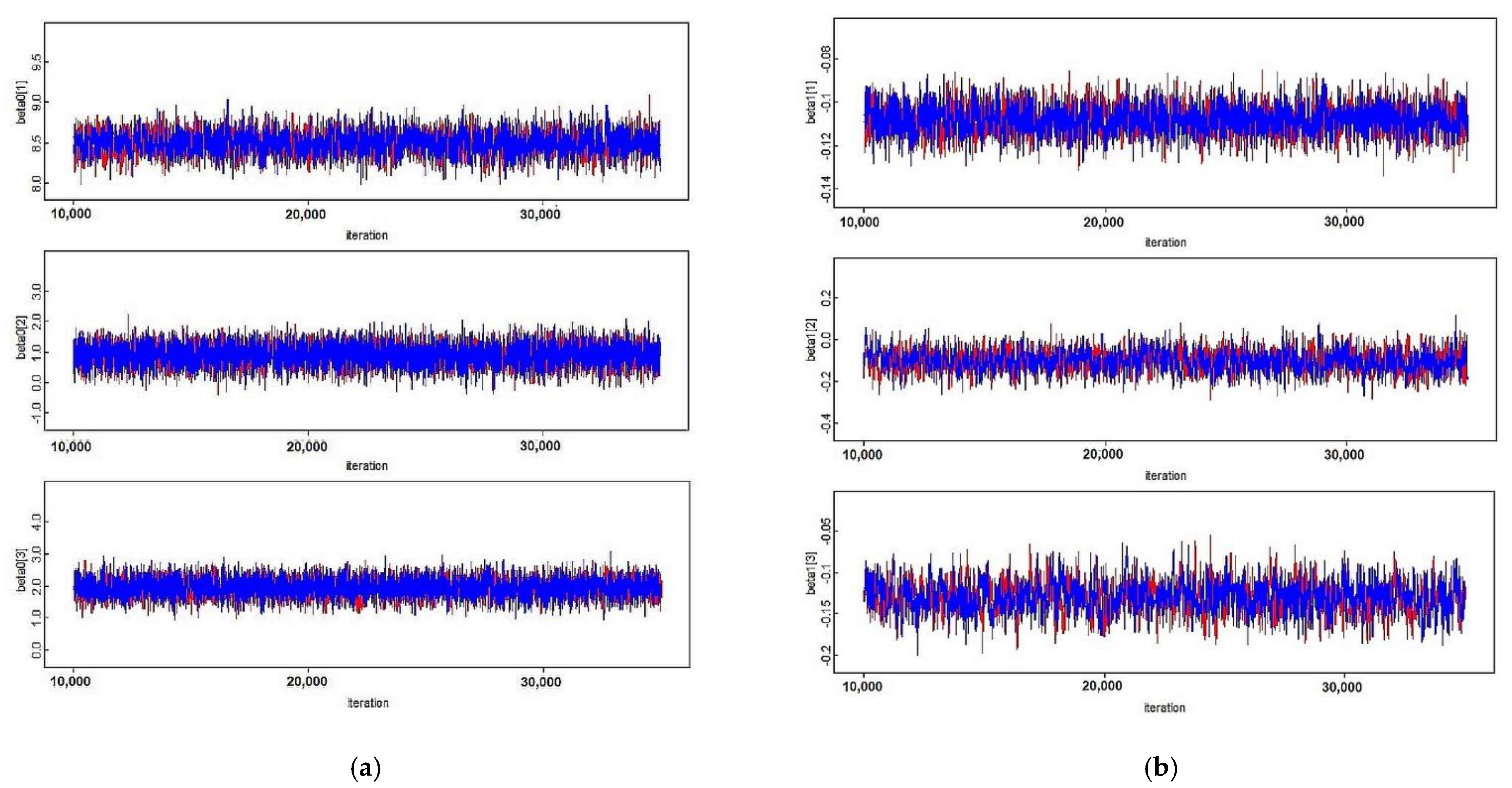
3.3. Convergence Diagnostics

In the Bayesian schemes, the convergence of MCMC simulation implies that the Markov chain attains the posterior distribution of parameters. The MCMC convergence condition can be shown graphically by the trace plot of MCMC dynamical movements. The trace plot outlines the number of iterations against the generated values of estimated parameters. If these values, which are inside a domain, do not have firm periodicities or tendencies, then it can be supposed that convergence is reached. In a practical manner, the trace plot which virtually has a “fat hairy caterpillar” like plot indicates a convergence of the Markov chain (Tatarinova and Schumitzky 2015). Other analytical methods that can be implemented to assess the convergence of MCMC are fully explained by Cowles and Carlin (1996). One of the analytical methods, the Gelman Rubin method, is recommended to be implemented during the estimation of the Bayesian model through MCMC simulation (Gelman and Shirley 2011).

The Gelman Rubin method constructs m mutually independent Markov chains, which assess its convergence by estimating the potential scale-reduction factor (PSRF). Every m Markov chains is convergent if the PSRF is less than 1.2 (Tatarinova and Schumitzky 2015). The implementation of convergence diagnostic methods for MCMC in the context of Bayesian mixture modeling is discussed in Suryaningtyas et al. (2018), Susanto et al. (2019), and Iriawan et al. (2019). All authors suggest that it should combine diagnostics methods with a graphical approach to determine the convergence condition of MCMC.

3.4. Model Selection

The Bayesian mixture models can be selected based on their out-of-sample predictive accuracy which can be estimated through information criteria approaches. Watanabe (2010) introduced the WAIC which is recommended for singular statistical models in which finite mixture models are classified into these models. The WAIC is formed by estimating the expected log pointwise predictive density (${\widehat{\mathrm{elppd}}}_{waic}$):

$${\widehat{\mathrm{elppd}}}_{waic}=\widehat{\mathrm{lppd}}-\widehat{p_{waic}}$$

(23)

where $\widehat{\mathrm{lppd}}$ is the estimation of the log pointwise predictive density, and $\widehat{p_{waic}}$ is the estimated effective number of parameters. $\widehat{\mathrm{lppd}}$ is defined by:

$$\widehat{\mathrm{lppd}}={\displaystyle \sum _{i=1}^n}\log \left(\frac{1}{s}{\displaystyle \sum _{s=1}^S}{h}_{log}\left(y_i|x_i,{\mathit{\vartheta }}^{(s)}\right)\right)$$

where S is the number of simulations performed and ${\mathit{\vartheta }}^{(s)}$ is the simulated values of parameter $\mathit{\vartheta }$ at the s-th iteration with $s=1,2,\dots ,S$. $\widehat{p_{waic}}$ is calculated based on the posterior sample variance of the log pointwise predictive density which is summed over all the data points $y_i$:

$$\widehat{p_{waic}}={\displaystyle \sum _{i=1}^n}\frac{1}{S-1}{\displaystyle \sum _{s=1}^S{\left(\log (h_{log}\left(y_i|x_i,{\mathit{\vartheta }}^{(s)}\right)-E\left[\log \left(h_{log}\left(y_i|x_i,{\mathit{\vartheta }}^{(s)}\right)\right)\right]\right)}^2}$$

(24)

Another version of $\widehat{p_{waic}}$ that can be used is constructed as a mean-based formula:

$$\widehat{p_{waic}}=2{\displaystyle \sum _{i=1}^n}\left(\log \left(\frac{1}{S}{\displaystyle \sum _{s=1}^S{h}_{log}\left(y_i|x_i,{\mathit{\vartheta }}^{(s)}\right)}\right)-\frac{1}{S}{\displaystyle \sum _{s=1}^S\log \left(h_{log}\left(y_i|x_i,{\mathit{\vartheta }}^{(s)}\right)\right)}\right)$$

(25)

The variance-based formula (24) is more appropriate for practical use than the mean-based formula (25) since the variance-based formula gives results closer to the leave-one-out cross-validation (LOO-CV) as a natural method for estimating the out-of-sample predictive accuracy. In our proposed model, the values of pointwise predictive density $h_{log}\left(y_i|x_i,{\mathit{\vartheta }}^{(s)}\right)$ are calculated for each observation from Equation (9) in which ${\mathit{\vartheta }}^{(s)}=({\mathit{\alpha }}^{(s)},{\mathit{\beta }}_1{}^{(s)},{\mathit{\beta }}_2{}^{(s)}\dots ,{\mathit{\beta }}_K{}^{(s)},w^{(s)}{)}^t$ are computed by Algorithm 1.

The WAIC can be defined as a deviance scale form by multiplying Equation (23) by −2:

$$\mathrm{WAIC}=-2{\widehat{\mathrm{elppd}}}_{waic}=-2\widehat{\mathrm{lppd}}+2\widehat{p_{waic}}$$

(26)

Equation (26) is suitable since it can be compared with other measures of deviance, e.g., AIC and DIC (Gelman et al. 2014). The WAIC value of a model cannot be interpreted without regarding the WAIC values of other models. From the viewpoint of predictive accuracy, the performance of the two models can be compared by measuring the difference in their WAIC values. If the difference is significantly large, then the model that has the lowest value of WAIC has better predictive accuracy than the others.

4. Real Data Applications

Faraway (2016) considers the GLMs with gamma-distributed responses to be appropriate in two conditions. First, if the response clearly has a gamma distribution, then the GLMs with gamma-distributed responses is certainly applicable. Second, if another condition is not sure about a statistical distribution of the response but supposes there is a relationship between the mean and the variance of the response. Thus, we use two real data applications that have a different typical distribution of response to show the specific performances of the Bayesian mixture of the log-link gamma GLMs.

In the first case, we study the modeling of the gross domestic product at purchasing power parity (GDP_PPP) per capita in 160 countries. GDP_PPP per capita as the response for the overall data as well as in each mixture component has a gamma distribution with no extreme values.

Conversely, in the second case, the household income data as the whole response are not identified as following a specific statistical distribution. Nevertheless, in each mixture component, the responses have different statistical distributions. In the first mixture component, the response has a generalized gamma distribution with four parameters, and in the other mixture components, the responses have lognormal distribution with three parameters. The data responses furthermore satisfy some essential properties such as being non-negative, continuous, positive-skewed, and the existence of linear relationships between the natural logarithm of the response and household characteristics as predictors. Such a case represented the implementation of the Bayesian mixture of the log-link gamma GLMs for modeling the responses that do not follow the gamma distribution but fulfil important characteristics that are needed to determine the model. Moreover, in this case, some extreme responses lay in each mixture component.

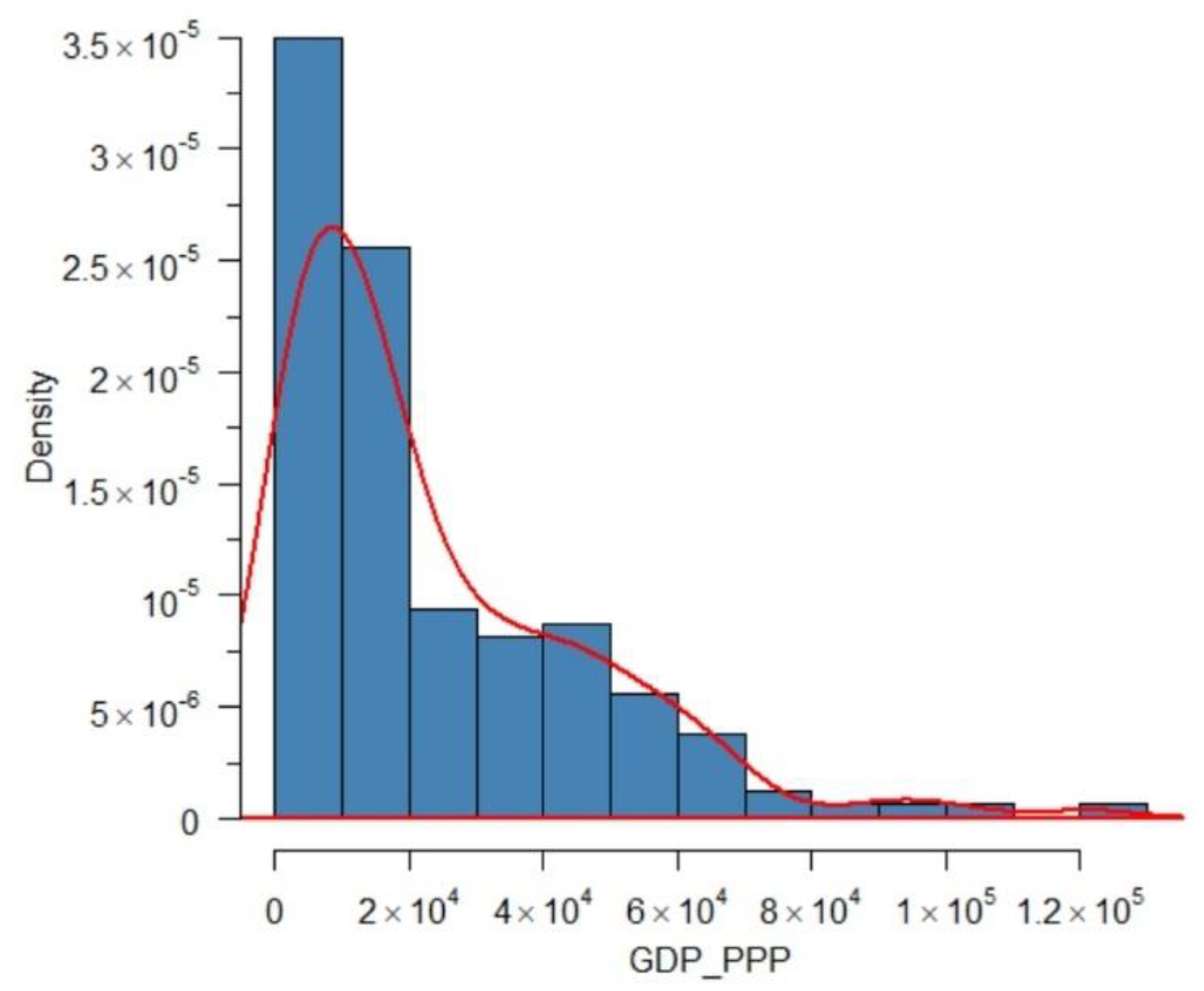
4.1. Modeling GDP_PPP

The GDP_PPP per capita gives gross domestic product per capita values in current international dollars transformed by purchasing power parity, which is a converter factor that can provide possibly determine economic comparisons between countries. For example the population weighted Gini ratio measure of income inequality based on GDP_PPP per capita can be used to assess intercountry income disparity (World Bank 2020). Other uses for purchasing power parity are recently considered by the World Bank (2021b).

We study the GDP_PPP per capita of 160 countries for 2019 as the response that is affected by the predictors of economic and social factors. There are four economic and social factors: number of populations, compulsory education years, gross domestics product (GDP), and corruption perception index (CPI). These countries are classified based on four economic groups: low, lower-middle, upper-middle, and high income (World Bank 2021a). We designate these groups as first, second, third, and fourth. Among the countries, there are 20, 42, 44, and 54 countries in the first, second, third, and fourth groups, respectively. The complete list of 160 countries can be seen in Appendix A.

4.1.1. Data Description

Data were obtained from World Development Indicators (WDI) of World Bank Open Data (2021) except for the CPI data, which were accessed from Transparency.org (2021). Before we apply our proposed model, we examine some data characteristics. Figure 2 shows the GDP_PPP per capita has a positive-skewed distribution which tends to follow a gamma distribution.

To achieve more accurate results, goodness-of-fit tests using the Kolmogorov-Smirnov and the Chi-Squared tests are conducted to verify a significant statistical distribution for the GDP_PPP per capita data. We set the null hypothesis, which state that the GDP_PPP per capita in whole data and in each group follow a gamma distribution.

Table 1. The goodness-of-fit tests.

Data	p-Value		Significant Statistical DISTRIBUTION
	Kolmogorov-Smirnov Test	Chi Squared Test
whole data	0.5419	0.1989	Gamma(1.06, 21,722)
first group	0.8673	0.8839	Gamma(7.52, 286.48)
second group	0.5166	0.8310	Gamma(3.97, 1750.3)
third group	0.9198	0.6462	Gamma(9.73, 1733.4)
fourth group	0.9507	0.7565	Gamma(5.90, 8259.4)

shows that all p-values are higher than a significance level of 0.05, which means that the null hypothesis is not rejected. It can be concluded that gamma distribution can be used to fit the GDP_PPP per capita for whole data and grouped data.

The implementation of the log-link gamma GLMs conceptually needs a linear relationship between the natural logarithm of the response and the predictors (Myers et al. 2012). The scatter plots displayed in Figure 3 represent the linear relationships between the natural logarithm of GDP_PPP per capita with the four predictors. The natural logarithm of GDP_PPP per capita has a linear relationship with the compulsory education years and the CPI. Other predictors, i.e., the number of populations and the GDP, do not have that linear relationship.

Therefore, we only assign the compulsory education years and the CPI as predictor variables in our proposed model, which has four mixture components representing the four economic groups. The model is defined by

$$h_{log}\left(y_i|x_i,\mathit{\vartheta }\right)={\displaystyle \sum _{k=1}^4}{w}_k{G}_k\left(y_i|{\alpha }_k,{\alpha }_k/{\mu }_{i_{k}k(log)}\right)$$

(27)

with $\mathit{\vartheta }=(\mathit{\alpha },{\mathit{\beta }}_1,{\mathit{\beta }}_2,{\mathit{\beta }}_3,{\mathit{\beta }}_4,w{)}^t$ and

$${\mu }_{i_{k}k(log)}=exp\left({\beta }_{0k}+{\beta }_{1k}eduyear{s}_{i_{k}k}+{\beta }_{2k}cp{i}_{i_{k}k}\right)$$

(28)

with $i_k=1,2,\dots ,n_k$ for $k$ = 1, 2, 3, 4, i.e., $n=n_1+n_2+n_3+n_4$. The predictor $eduyear{s}_{i_{k}k}$ denotes the compulsory education years in the i-th country in the k-th economics group. The predictor $cp{i}_{i_{k}k}$ denotes the CPI on the i-th country in the k-th economics group.

4.1.2. Estimated Parameters

The estimation processes perform 20,000 samples from two Markov chains that are eliminated in the first 1000 sample iterations in each chain as a burn-in stage. The prior distributions are constructed for three parameters that have to be estimated: the shape parameter $\mathit{\alpha }$, the mixing parameter $w$, and the coefficient ${\beta }_{jk}$. Regarding the pattern of distribution in Figure 1, the goodness-of-fit test in Table 1, and the proposed prior (16), we use the prior distribution for ${\alpha }_k$ by

$${\alpha }_k\sim Gamma(6,1)$$

for $k$ = 1, 2, 3, 4; ${\alpha }_k$ has a gamma distribution with a shape parameter of 6 and an inverse scale parameter of 1. Referring to the conjugate prior on (18), the mixing parameter $w$ has a Dirichlet distribution as a prior distribution with value 1 for all parameters:

$$w\sim Dir(1,1,1,1)$$

The equal value of parameters on that Dirichlet distribution, $Dir(1,1,1,1)$, implies a uniform distribution over the three-dimensional simplex. Concerning the prior distribution for ${\beta }_{jk}$, which is formed based on (17) according to our empirical studies, a large variance of ${\sigma }^2$, i.e., a noninformative prior for ${\beta }_{jk}$, can lead to no regularization on coefficient estimation. Consequently, the variance ${\sigma }^2$ needs to be relatively close to a zero mean; hence, the prior distributions for ${\beta }_{jk}$ consists of

$$\begin{gathered} {\beta }_{0k}\sim N(0,1) \\ {\beta }_{1k}\sim N(0,0.01) \\ {\beta }_{2k}\sim N(0,1) \end{gathered}$$

for $k$ = 1, 2, 3, 4. The detailed estimated results can be seen in

Table 2. The estimated parameters of the first, second, third, and fourth mixture components.

Mixture Component	Estimated Parameter	Estimated Value	95% Posterior Credible Interval		PSRF	Prior Distribution
			Lower	Upper
First	${\widehat{\alpha }}_1$	4.7110	2.3760	8.1820	1	${\alpha }_1\sim G(6,1)$
	${\widehat{w}}_1$	0.1279	0.0813	0.1830	1	$w_1\sim Dir(1,1,1,1)$
	${\widehat{\beta }}_{01}$	6.0850	4.8980	7.1260	1	${\beta }_{01}\sim N(0,1)$
	${\widehat{\beta }}_{11}$	0.1373	0.0365	0.2532	1	${\beta }_{11}\sim N(0,0.01)$
	${\widehat{\beta }}_{21}$	0.0179	−0.004	0.0455	1	${\beta }_{21}\sim N(0,1)$
Second	${\widehat{\alpha }}_2$	4.8840	3.0920	7.2460	1	${\alpha }_2\sim G(6,1)$
	${\widehat{w}}_2$	0.2621	0.1977	0.3315	1	$w_2\sim Dir(1,1,1,1)$
	${\widehat{\beta }}_{02}$	6.4750	5.5900	7.2510	1	${\beta }_{02}\sim N(0,1)$
	${\widehat{\beta }}_{12}$	0.1354	0.0811	0.1918	1	${\beta }_{12}\sim N(0,0.01)$
	${\widehat{\beta }}_{22}$	0.0314	0.0109	0.0545	1	${\beta }_{22}\sim N(0,1)$
Third	${\widehat{\alpha }}_3$	7.500	4.7750	11.030	1	${\alpha }_3\sim G(6,1)$
	${\widehat{w}}_3$	0.2742	0.2087	0.3488	1	$w_3\sim Dir(1,1,1,1)$
	${\widehat{\beta }}_{03}$	8.913	8.2900	9.4530	1	${\beta }_{03}\sim N(0,1)$
	${\widehat{\beta }}_{13}$	0.0391	0.0003	0.0787	1	${\beta }_{13}\sim N(0,0.01)$
	${\widehat{\beta }}_{23}$	0.0106	0.0005	0.0214	1	${\beta }_{23}\sim N(0,1)$
Fourth	${\widehat{\alpha }}_4$	7.4700	4.8990	10.790	1	${\alpha }_4\sim G(6,1)$
	${\widehat{w}}_4$	0.3358	0.2650	0.4103	1	$w_4\sim Dir(1,1,1,1)$
	${\widehat{\beta }}_{04}$	9.0980	8.3280	9.4530	1.01	${\beta }_{04}\sim N(0,1)$
	${\widehat{\beta }}_{14}$	0.0220	−0.029	0.0768	1	${\beta }_{14}\sim N(0,0.01)$
	${\widehat{\beta }}_{24}$	0.0221	0.0154	0.0295	1.01	${\beta }_{24}\sim N(0,1)$

.

In Table 2, the estimated values of parameters have a 95% posterior credible interval and a related diagnostic measurement of MCMC convergence, i.e., the PSRF. All PSRF values less than 1.2 ensure that the two Markov chains are convergent to achieve the posterior distribution of the parameters. Figure 4 confirms the convergence of two Markov chains for ${\widehat{\beta }}_{1k}$ and ${\widehat{\beta }}_{2k}$.

The posterior predictive check can be conducted for model checking purposes by determining the graphical posterior predictive checks. The graphical posterior predictive check that displays the observed data alongside the replicated data regenerated from the fitted model can show systematic differences between the observed and replicated data. Other methods that are useful for checking Bayesian models are discussed by Lunn et al. (2013). Figure 5 presents the distribution of observed and replicated data to show the adequacy of log-link gamma GLMs for fitting observed data.

In the Bayesian framework, a 95% posterior credible interval means that the actual probability of having true values of the estimated parameter in that interval is 0.95. Therefore, it can be applied as an assessment tool to determine the significance of the estimated parameter, which can be considered significant if the 95% posterior credible interval does not include a zero value. The 95% posterior credible intervals of two estimated parameters, ${\widehat{\beta }}_{21}$ and ${\widehat{\beta }}_{14}$, contain zero values indicating that the ${\widehat{\beta }}_{21}$ and ${\widehat{\beta }}_{14}$ are not significant for the model. The estimated ${\widehat{\beta }}_{21}$, which is not significant, means that the predictor CPI does not have an effect on the GDP_PPP per capita in the low-income country group, because the compulsory education years has a positive effect on the GDP_PPP per capita. On the other hand, among high-income countries, it is not significantly influenced by compulsory education since the estimated ${\widehat{\beta }}_{14}$ can have a zero value. The CPI, even only slightly, still has a positive influence on the GDP-PPP per capita. In the lower-middle and upper-middle country groups, the compulsory education years and the CPI have a positive influence on the GDP_PPP per capita.

Concerning comparative studies, we take two models: the Bayesian mixture of linear regression model as a simpler mixture of regression model and the Bayesian gamma regression model as a model without a finite mixture framework. The Bayesian mixture of linear regression model is given by

$$h\left(y_i|x_i,\mathit{\vartheta }\right)={\displaystyle \sum _{k=1}^4}{w}_k{N}_k\left(y_i|{\mu }_{i_{k}k},{\sigma }_k{}^2\right)$$

with $N_k(.)$ as a normal distribution in the k-th mixture component and

$${\mu }_{i_{k}k}={\beta }_{0k}+{\beta }_{1k}eduyear{s}_{i_{k}k}+{\beta }_{2k}cp{i}_{i_{k}k}$$

The prior distributions for ${\beta }_{jk}$ and the standard deviations ${\sigma }_k$ consists of

$$\begin{gathered} {\sigma }_k\sim U(0,8000) \\ {\beta }_{0k}\sim N(0,1\times {10}^6) \\ {\beta }_{1k}\sim N(0,1\times {10}^4) \\ {\beta }_{2k}\sim N(0,1000) \end{gathered}$$

where ${\sigma }_k\sim U(0,8000)$ means the standard deviations ${\sigma }_k$ are distributed uniformly between 0 and 8000, for k = 1, 2, 3, 4. The estimate procedures run 20,000 samples from two Markov chains, with the first 600 sample iterations in each chain discarded as a burn-in stage. The estimated parameters for the Bayesian mixture of linear regression model are presented on

Table 3. The estimated parameters of the Bayesian mixture of linear regression model.

Mixture Component	Estimated Parameter	Estimated Value	95% Posterior Credible Interval		PSRF	Prior Distribution
			Lower	Upper
First	${\widehat{\sigma }}_1$	1043	820.1	1347	1	${\sigma }_1\sim U(0,8000)$
	${\widehat{w}}_1$	0.2139	0.154	0.2799	1	$w_1\sim Dir(1,1,1,1)$
	${\widehat{\beta }}_{01}$	1180	40.68	2391	1	${\beta }_{01}\sim N(0,1\times {10}^6)$
	${\widehat{\beta }}_{11}$	102.2	−17.68	218.5	1	${\beta }_{11}\sim N(0,1\times {10}^4)$
	${\widehat{\beta }}_{21}$	23.82	−5.616	53.78	1	${\beta }_{21}\sim N(0,1000)$
Second	${\widehat{\sigma }}_2$	3573	2917	4403	1	${\sigma }_2\sim U(0,8000)$
	${\widehat{w}}_2$	0.3357	0.2661	0.4097	1	$w_2\sim Dir(1,1,1,1)$
	${\widehat{\beta }}_{02}$	3059	1489	4665	1	${\beta }_{02}\sim N(0,1\times {10}^6)$
	${\widehat{\beta }}_{12}$	311.9	163	458.4	1	${\beta }_{12}\sim N(0,1\times {10}^4)$
	${\widehat{\beta }}_{22}$	108.3	64.75	151.2	1	${\beta }_{22}\sim N(0,1000)$
	${\widehat{\sigma }}_3$	7644	6762	7990	1	${\sigma }_3\sim U(0,8000)$
	${\widehat{w}}_3$	0.2008	0.1429	0.2648	1	$w_3\sim Dir(1,1,1,1)$
Third	${\widehat{\beta }}_{03}$	4344	2515	6160	1	${\beta }_{03}\sim N(0,1\times {10}^6)$
	${\widehat{\beta }}_{13}$	418.1	241.2	594	1	${\beta }_{13}\sim N(0,1\times {10}^4)$
	${\widehat{\beta }}_{23}$	188.4	138	238.6	1	${\beta }_{23}\sim N(0,1000)$
	${\widehat{\sigma }}_4$	7963	7864	7999	1	${\sigma }_4\sim U(0,8000)$
	${\widehat{w}}_4$	0.2496	0.1868	0.3183	1	$w_4\sim Dir(1,1,1,1)$
Fourth	${\widehat{\beta }}_{04}$	6617	4760	8490	1	${\beta }_{04}\sim N(0,1\times {10}^6)$
	${\widehat{\beta }}_{14}$	627.4	444	809	1	${\beta }_{14}\sim N(0,1\times {10}^4)$
	${\widehat{\beta }}_{24}$	467.7	428.1	508	1	${\beta }_{24}\sim N(0,1000)$

.

Table 3 reveals that the predictors, eduyears and cpi, do not affect the response in the first mixture component. It can be observed that two estimated parameters, ${\widehat{\beta }}_{11}$ and ${\widehat{\beta }}_{21}$, have 95% posterior credible intervals that contain zero values.

The modeling of GDP_PPP per capita can be developed without regard to the four economic groups. In such a case, the Bayesian gamma regression model can be implemented without having a finite mixture framework. The gamma regression model is specified by

$$y_i\sim Gamma(\alpha ,\alpha /{\mu }_i)$$

where

$${\mu }_i=exp\left({\beta }_0+{\beta }_{1}eduyear{s}_i+{\beta }_{2}cp{i}_i\right)$$

Similar prior distributions and processes for MCMC simulation in the Bayesian mixture of the log-link gamma GLMs are implemented for inferencing the Bayesian gamma regression model. The estimated parameters of the Bayesian gamma regression model can be seen in

Table 4. The estimated parameters of the Bayesian gamma regression model.

Estimated Parameter	Estimated Value	95% Posterior Credible Interval		PSRF	Prior Distribution
		Lower	Upper
$\widehat{\alpha }$	2.2160	1.7990	2.6990	1	$\alpha \sim Gamma(6,1)$
${\widehat{\beta }}_0$	7.1270	6.6560	7.5760	1	${\beta }_0\sim N(0,1)$
${\widehat{\beta }}_1$	0.0798	0.0356	0.1251	1	${\beta }_1\sim N(0,0.01)$
${\widehat{\beta }}_2$	0.0413	0.0353	0.0471	1	${\beta }_2\sim N(0,1)$

. The signs of the coefficients ${\widehat{\beta }}_0$, ${\widehat{\beta }}_1$, and ${\widehat{\beta }}_2$ are positive, which signifies that the enhancement of the compulsory education years and the improvement of the corruption perception index will increase the GDP_PPP per capita.

We take a comparative study between the fitted Bayesian gamma regression model, the fitted Bayesian mixture of linear regression model as a simpler mixture model, and the fitted Bayesian mixture of the log-link gamma GLMs in predictive performance by computing the WAIC value.

Table 5. The WAIC values of the model for GDP_PPP case.

Fitted Model	WAIC
Bayesian mixture of the log-link gamma GLMs	3231
Bayesian mixture of linear regression	3341
Bayesian gamma regression	3411

displays the WAIC value for the fitted Bayesian mixture of the log-link gamma GLMs, which is smaller than the WAIC values of the fitted Bayesian gamma regression model and the fitted Bayesian mixture of linear regression model. Thus, in the predictive capability aspect, the fitted Bayesian mixture of the log-link gamma GLMs is better than the fitted Bayesian gamma regression model and the fitted Bayesian mixture of linear regression model.

To find out the predictive capability more comprehensively, we apply both models to predict future GDP_PPP values for 2020. The density plots of predicted results are compared graphically with the observed data of GDP_PPP in 2020 that are obtained from World Bank Open Data (2022). Figure 6 represents the density plots that can exhibit some differences between the predicted results and the observed data.

It can be seen from Figure 6 that the fitted Bayesian mixture of the log-link gamma GLMs has a better performance than the fitted Bayesian mixture of linear regression model and the fitted Bayesian gamma regression model in predicting future GDP_PPP values in 2020.

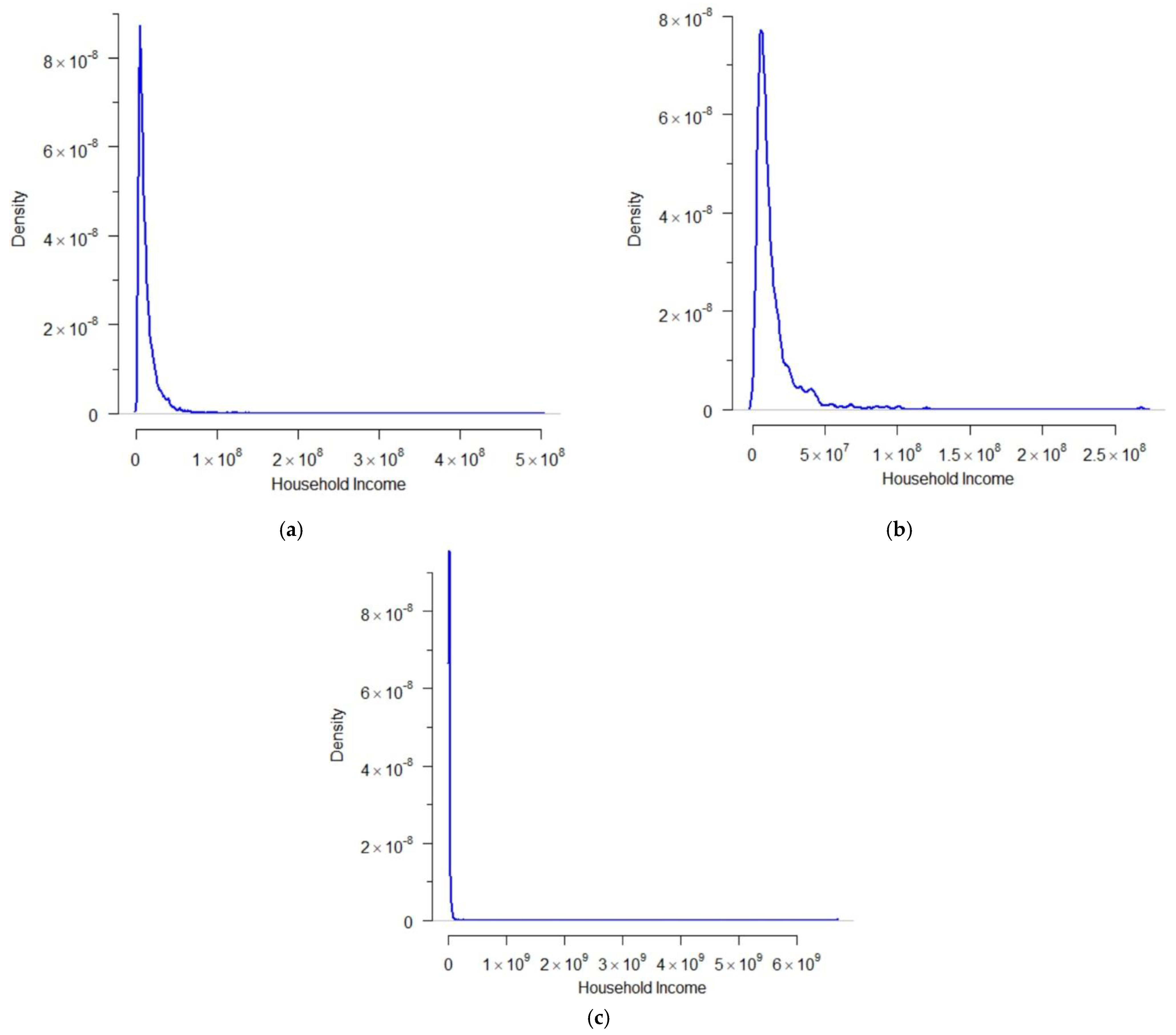
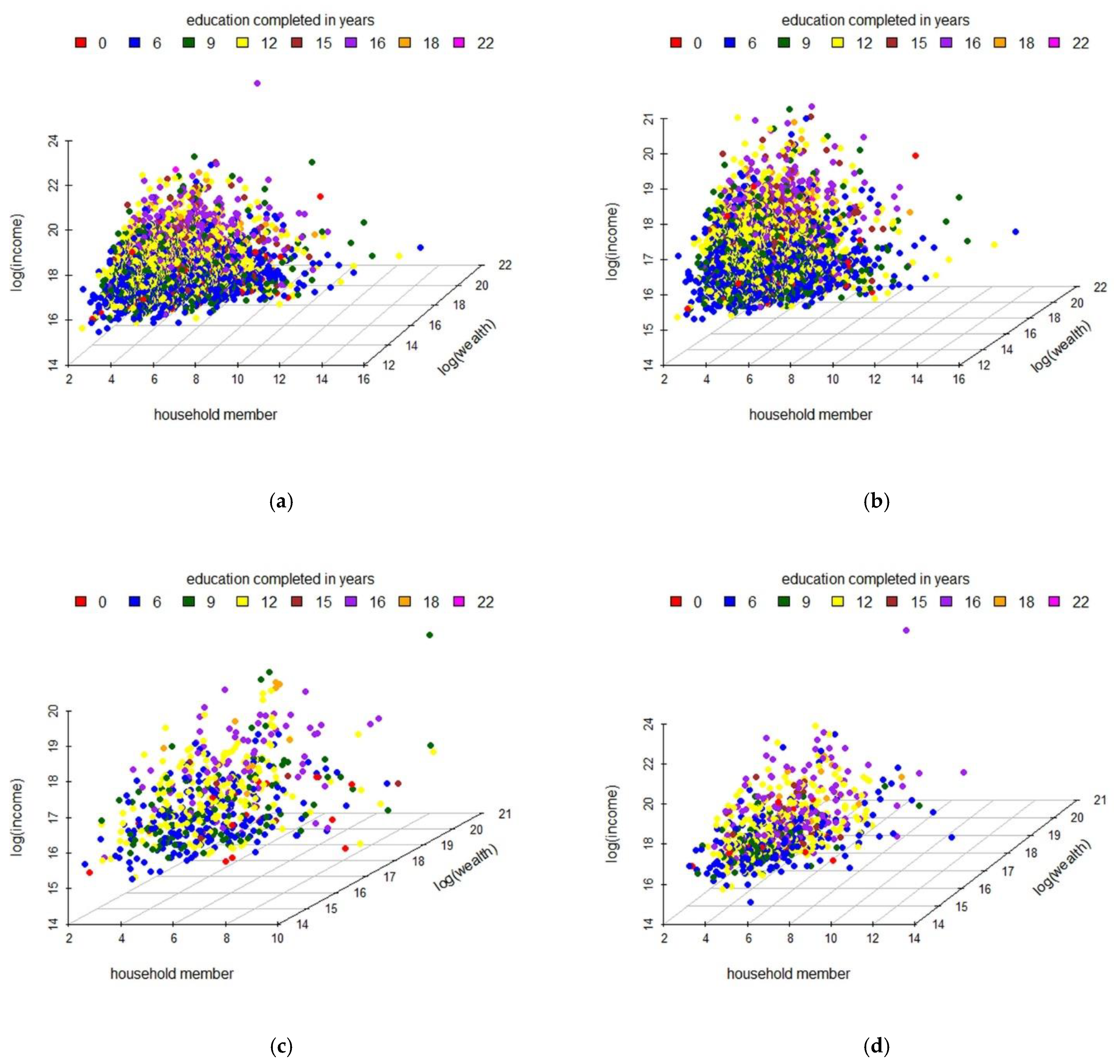
4.2. Modeling Household Income

In the field of income distribution analysis, the density function of income distribution can be used as an important approach to verify economic inequality. A functional form of the density function is determined to obtain a specific model that can exhibit the reality about income distribution, so inequality analyses can be built in terms of that specific model. Since the functional form of the density function is generally unknown, it needs to be estimated. Cowell and Flachaire (2015) remarked that the finite mixture model could be more convenient for estimating the density function of income distributions. They started to describe conceptually the implementation of the finite mixtures of linear regression for analyzing income distributions. However, the finite mixture of GLMs was not carried out in their studies.

The dynamics of household income as a fundamental element of income inequality can affect economic growth. Some researchers studied interrelated topics on household income, income inequality, and economic growth. Causa et al. (2014) found that improved growth in household income reduced income inequality. Meanwhile, Stiglitz (2015) stated that immoderate inequality could cause inadequate economic performance.

4.2.1. Data Description

We research the annual household income per capita in six economic corridors based on the Masterplan for Accelerating and Expansion of Indonesia Economic Development 2011–2025 (Coordinating Ministry for Economic Affairs 2011). The corridors consist of the six main regions of Indonesia: Sumatra, Java, Kalimantan, Sulawesi, Bali-Nusa Tenggara, and Papua-Maluku. Alisjahbana (2011) grouped corridors into three groups comprising two economic corridors in each. The first group consisted of Sumatra and Java; the second group, Kalimantan and Sulawesi, and the third, Bali-Nusa Tenggara and Papua-Maluku. In our research, we construct three mixture components representing the three groups. We develop our model from the point of view proposed by Chotikapanich et al. (2012). They constructed the income distribution of the whole region, which could be represented as a mixture model with subset regions as a member of the mixture component.

Household income data were determined from The Fifth Wave of the Indonesia Family Life Survey (IFLS-5) 2014 (Strauss et al. 2016). We sample 5545 households from 23 provinces in the six economic corridors. In more detail, 4, 267, 586, and 692 households are members of the first, second, and third groups, respectively. Our verification of the whole household income data using the Kolmogorov-Smirnov test indicates that it does not pursue a specific statistical distribution. However, once we examine the data in each mixture component, the response in the first mixture has a generalized gamma distribution with four parameters and a lognormal distribution with three parameters for responses in the other mixture components. Therefore, we need to determine an appropriate statistical distribution suitable for modeling household income data.

Some essential patterns such as non-negative, continuous, and positive-skewed are present in the household income data which are displayed in Figure 7. It shows the possibility of proposing gamma distribution as a representative statistical distribution for household income data. Figure 8 exhibits the scatter plots in four dimensions which relate the natural logarithm of household income data to all three predictors; the number of household members, the number of completed years of formal education by the head of the household, and the natural logarithm of the household’s wealth. The scatter plots indicate a linear relationship between the natural logarithm of household income data and all three predictors which exist in the overall response data in Figure 8a and in each mixture component shown in Figure 8b–d. These relationships give evidence that it can be modeled by the log-link gamma GLMs.

The performance of the gamma GLM was studied by Fu and Moncher (2004) who verified the unbiasedness and stability of the GLM for non-negative, continuous, and positive-skewed data. They found that the GLM assuming the gamma distribution gave better predictive accuracy and efficiency than the GLM assuming the normal distribution or the lognormal distribution. Thus, we consider that the gamma GLM is a reasonable model for analyzing household income data.

Previously, Wicaksono et al. (2017) showed that the natural log of annual household income per capita as a response variable had been regressive on household characteristics as predictors. Nonetheless, they worked under the assumption that the household income data followed a normal distribution, and their model did not use the finite mixture modeling framework.

4.2.2. Estimated Parameters

In the k-th mixture component, $k$ = 1, 2, 3, we consider that annual household income per capita that related to household characteristics can be modeled by a log-link gamma GLM. Referring to Equation (9), the finite mixture model used in this study is defined as

$$\begin{array}{ll}{h}_{log}\left(y_i|x_i,\mathit{\vartheta }\right)=\hfill & w_1{G}_1\left(y_{i_{1}1}|{\alpha }_1,{\alpha }_1/{\mu }_{i_{1}1(log)}\right)+w_2{G}_2\left(y_{i_{2}2}|{\alpha }_2,{\alpha }_2/{\mu }_{i_{2}2(log)}\right)\hfill \\ \hfill & +w_3{G}_3\left(y_{i_{3}3}|{\alpha }_3,{\alpha }_3/{\mu }_{i_{3}3(log)}\right),\hfill \end{array}$$

(29)

where $\mathit{\vartheta }=(\mathit{\alpha },{\mathit{\beta }}_1,{\mathit{\beta }}_2,{\mathit{\beta }}_3,w{)}^t$. The variable $y_i$ denotes annual household income per capita on the i-th household observations which are specified, namely, $y_{i_{1}1}$, $y_{i_{2}2}$, and $y_{i_{3}3}$ for the i-th household observations included in the first, second, and third mixture components, respectively. Thus, for all observations $i=1,2,\dots ,5545$, $i_k=1,2,\dots ,n_k$ with $k$ = 1, 2, 3, i.e., $n=n_1+n_2+n_3$.

The function ${\mu }_{i_{1}1(log)}$, ${\mu }_{i_{2}2(log)}$, and ${\mu }_{i_{3}3(log)}$ are defined as

$${\mu }_{i_{1}1(log)}=exp\left({\beta }_{01}+{\beta }_{11}{x}_{i_{1}11}+{\beta }_{21}{x}_{i_{2}21}+{\beta }_{31}{x}_{i_{3}31}\right)$$

(30)

$${\mu }_{i_{2}2(log)}=exp\left({\beta }_{02}+{\beta }_{12}{x}_{i_{2}12}+{\beta }_{22}{x}_{i_{2}22}+{\beta }_{32}{x}_{i_{2}32}\right)$$

(31)

and

$${\mu }_{i_{3}3(log)}=exp\left({\beta }_{03}+{\beta }_{13}{x}_{i_{3}13}+{\beta }_{23}{x}_{i_{3}23}+{\beta }_{33}{x}_{i_{3}33}\right)$$

(32)

The predictors on each mixture component of Equations (30)–(32) are defined as follows: $x_{i_{k}1k}$ is the number of household member; $x_{i_{k}2k}$ is the number of completed years of formal education by the head of the household; and $x_{i_{k}3k}$ is the natural logarithm of the household’s wealth (in Indonesian rupiah per year) with $k$ = 1, 2, 3. We take two Markov chains with 25,000 iterations on each chain that are discarded during the first 10,000 iterations as burn-in. Thus, we use 50,000 samples to estimate the parameters.

The prior distributions are set up for the shape parameter $\mathit{\alpha }$, the mixing parameter $w$, and the coefficient ${\beta }_{jk}$. Referring to the pattern of distribution in Figure 3 and the proposed prior (16), we use the prior distribution for ${\alpha }_k$:

$${\alpha }_k\sim Gamma(2,1)$$

where ${\alpha }_k$ has a gamma distribution with a shape parameter of 2 and an inverse scale parameter of 1.

The mixing parameter $w$ has a Dirichlet distribution as a prior distribution with value of 1 for all parameters,

$$w\sim Dir(1,1,1)$$

The equal value of parameters on that Dirichlet distribution, $Dir(1,1,1)$, implies a uniform distribution over the two-dimensional simplex. The prior of ${\beta }_{jk}$ is specified based on (17). Accordingly, we propose the small variance ${\sigma }_2=0.1$; thus, the prior distribution for ${\beta }_{jk}$ is

$${\beta }_{0k},{\beta }_{jk}\sim N(0,0.1)$$

for $j=1,2,3$ and $k=1,2,3.$ The implementation of the prior distribution N(0,0.1) suggests that the corresponding predictors ${\beta }_{jk}$ have fewer effects on the posterior distribution ${\beta }_{jk}$. This arrangement scheme of prior distribution allows a data-driven approach, i.e., the likelihood is more dominant than the prior distribution throughout the computation of the posterior distribution. The results are provided in

Table 6. The estimated parameters of the first, second, and third mixture components.

Estimated Parameter and Coefficient	Estimated Value	95% Posterior Credible Interval		Markov Chain Error	PSRF
		Lower	Upper
${\widehat{\alpha }}_1$	2.2740	2.1820	2.3670	0.0002	1
${\widehat{\alpha }}_2$	0.5182	0.4701	0.5688	0.0001	1
${\widehat{\alpha }}_3$	1.6270	1.4690	1.7910	0.0004	1
${\widehat{w}}_1$	0.7693	0.7581	0.7804	0.0000	1
${\widehat{w}}_2$	0.1058	0.0978	0.114	0.0000	1
${\widehat{w}}_3$	0.1249	0.1164	0.1338	0.0000	1
${\widehat{\beta }}_{01}$	8.4930	8.2150	8.7630	0.0029	1
${\widehat{\beta }}_{02}$	0.8892	0.2691	1.5140	0.0034	1
${\widehat{\beta }}_{03}$	1.9470	1.4240	2.4710	0.0032	1
${\widehat{\beta }}_{11}$	−0.1080	−0.1205	−0.0953	0.0001	1
${\widehat{\beta }}_{12}$	−0.1013	−0.1993	−0.0035	0.0012	1
${\widehat{\beta }}_{13}$	−0.1298	−0.1657	−0.0926	0.0005	1
${\widehat{\beta }}_{21}$	0.0321	0.0262	0.0379	0.0000	1
${\widehat{\beta }}_{22}$	0.1679	0.1315	0.2014	0.0004	1
${\widehat{\beta }}_{23}$	0.0172	0.0013	0.0332	0.0001	1
${\widehat{\beta }}_{31}$	0.4710	0.4539	0.4889	0.0001	1
${\widehat{\beta }}_{32}$	0.8904	0.8375	0.9452	0.0005	1
${\widehat{\beta }}_{33}$	0.8685	0.8319	0.9049	0.0003	1

.

It can be noted from Table 6 that all of the estimated parameters are significant at a 95% posterior credible interval. It can be shown that for all estimated parameters, the values of PSRF that are equal to 1 confirm that the Markov chains for all estimated parameters are convergent. Figure 9, which represents the trace plot of the Markov chains for estimated coefficients ${\widehat{\mathit{\beta }}}_0$, ${\widehat{\mathit{\beta }}}_1$, ${\widehat{\mathit{\beta }}}_2$, and ${\widehat{\mathit{\beta }}}_3$, proves the convergences.

The estimated shape parameters $\mathit{\alpha }$ (2.2740, 0.5182, and 1.6270) for the first, second and third groups, respectively, closely fit the distribution pattern of annual household income per capita in each mixture component, and the mixing parameters are 0.7693, 0.1058, and 0.1249, respectively. In this case, the mixing parameter represents the proportion of households in the groups against the sample populations. The sign of the estimated coefficients ${\widehat{\mathit{\beta }}}_0$, ${\widehat{\mathit{\beta }}}_1$, ${\widehat{\mathit{\beta }}}_2$, and ${\widehat{\mathit{\beta }}}_3$ are as expected for each of the groups. The negative sign for ${\widehat{\mathit{\beta }}}_1$ suggests that the increasing number of household members reduces the annual household income per capita. The length of education by the head of the household positively correlates with the annual household income per capita, indicating positive sign for ${\widehat{\mathit{\beta }}}_2$. It implies that knowledge may improve as the length of education by the head of household rise, thereby resulting in higher annual household income per capita. The household’s wealth also has a positive relationship to the annual household income per capita. This relation is generally reasonable since households with more wealth can generate more income using their own wealth. The results show that the Bayesian-MCMC approach gives a suitable result for estimating a finite mixture of the log-link gamma GLMs. The distribution of observed and replicated data depicting a graphical posterior predictive check in Figure 10 shows that the fitted model generally matches the observed data.

To learn the capability of predictive accuracy, the fitted Bayesian mixture of the log-link gamma GLMs is compared with the fitted Bayesian gamma regression model by calculating the WAIC. The gamma regression model is given by:

$$y_i\sim Gamma(\alpha ,\alpha /{\mu }_i)$$

with

$${\mu }_i=exp\left({\beta }_0+{\beta }_1{x}_{i1}+{\beta }_2{x}_{i2}+{\beta }_3{x}_{i3}\right)$$

The estimated parameters of the Bayesian gamma regression model shown in Table 6 are determined through the Gibbs sampler algorithm with the same prior distributions which are used to infer the fitted Bayesian mixture of the log-link gamma GLMs:

$$\alpha \sim Gamma(2,1)$$

and

$${\beta }_0,{\beta }_j\sim N(0,0.1)$$

Similar processes for MCMC simulations are also conducted with two Markov chains with 25,000 iterations discarded in the first 10,000 iterations as burn-in, so it uses 50,000 samples. Based on the PSRF values in

Table 7. The estimated parameters of the Bayesian gamma regression model.

Estimated Parameter and Coefficient	Estimated Value	95% Posterior Credible Interval		Markov Chain Error	PSRF
		Lower	Upper
$\widehat{\alpha }$	1.3920	1.3440	1.4400	0.0001	1
${\widehat{\beta }}_0$	7.6290	7.3250	7.9360	0.0030	1
${\widehat{\beta }}_1$	−0.1092	−0.1241	−0.0941	0.0001	1
${\widehat{\beta }}_2$	0.0539	0.0472	0.0608	0.0000	1
${\widehat{\beta }}_3$	0.5178	0.4976	0.5375	0.0002	1

, the estimated parameters are convergent to their posterior distributions, whereas the 95% posterior credible intervals indicate that all estimated parameters are significant.

However, the WAIC value of the Bayesian gamma regression, which has an infinite value as shown in

Table 8. The WAIC values of the model for household income case.

Fitted Model	WAIC
Bayesian mixture of the log-link gamma GLMs	192,200
Bayesian gamma regression	infinity

, indicates that the Bayesian mixture of the log-link gamma GLMs is significantly better in the predictive accuracy than the Bayesian gamma regression model.

5. Discussion

Two examples of real-data applications have a different typical distribution of response data. In the first example, the modeling of GDP_PPP per capita following the gamma distribution, the Bayesian mixture of the log-link gamma GLMs considerably outperforms the Bayesian mixture of linear regression model and the Bayesian gamma regression based on the predictive measure of WAIC. Moreover, through the finite mixture framework, we discover the factual relationship between the GDP_PPP per capita and the predictors in each group. In low-income countries, only the compulsory education years has a significant effect on the GDP_PPP per capita. Conversely, only the CPI has an important contribution to the change in GDP_PPP per capita in high-income countries. In this case, the usefulness of the Bayesian mixture of the log-link gamma GLMs can be noted.

The second case, in addition to revealing the implementation of the model on the data that does not comply with the gamma distribution, exposes the influential presence of extreme values which can be regarded as outliers that can be eliminated from data or remain preserved in the data depending on their characteristics. Nevertheless, the existence of plentiful outliers in the data distribution was natural in the heavy-tailed distribution perspective (Klebanov and Volchenkova 2019). Hence, the outliers that exist in the household income data of the IFLS-5 do not need to be removed since they present an actual condition.

Referring to Equations (24)–(26), we find out that one of the possible sources in which the WAIC can have a large value is in the extreme values in the data distribution of $y_i$ that have a heavy-tailed distribution. Klebanov and Volchenkova (2019) showed that the observations belonging to the tail in a heavy-tailed distribution, i.e., extreme values, can have an infinite variance. To verify the existence of extreme values, we examine the adjusted boxplot, which is a modification of the boxplot used to depict a robust measure of skewness (Hubert and Vandervieren 2008). The adjusted boxplots displayed in Figure 11 describe some extreme values that exist in the household income data.

While more specifically, if we divide the data following the three mixture components as our proposed model, some extreme values will also be split into each mixture component. It will cause a difference in the WAIC value which is substantively wide between the fitted Bayesian gamma regression model and the fitted Bayesian mixture of the log-link gamma GLMs.

Several improvements for further studies related to the topic of this paper can be made for future research purposes. Inferential processes discussed in this paper use the Gibbs sampler algorithm through the MultiBUGS software. Further research can be developed by using the Hamiltonian Monte Carlo algorithm (HMC) with the no-U-turn (NUTS) sampler through the Stan software. Solikhah et al. (2021) showed that HMC using NUTS sampler performed well in estimating parameters of a mixture of K-component Fisher’s z autoregressive models. In addition, the proposed model can be developed for a mixture of distributions with more general gamma regression models with mean and shape (or variance) parameters following regression structures previously studied in Corrales and Cepeda-Cuervo (2019).

6. Conclusions

In this paper, we examine more extensively a Bayesian mixture of GLMs with gamma-distributed responses that combined three main parts: the GLMs with gamma-distributed response, finite mixture modeling, and a computational procedure for inferencing through the Bayesian-MCMC approach. Two link functions which are available for GLMs with gamma-distributed responses can give different results on the predictive mean, the log-link function is more appropriate than the inverse-link function to ensure the positivity of the predictive mean. Considering the implementation of the model on two real data applications, the link function used and the chosen prior distributions give an important role for the Bayesian-MCMC approach to work appropriately throughout the simulation-based inferential processes. We note some advantages of the Bayesian mixture of the log-link gamma GLMs. The model has better predictive accuracy than the Bayesian mixture of linear regression and the Bayesian gamma regression model. It can point out real relationships between the response and the predictors. Furthermore, it handles the problems concerning extreme values, whereas the Bayesian model without finite mixture framework has difficulty overcoming extreme values. Nevertheless, our research only uses the Gibbs sampler algorithm and the mixing parameter which is not a function of the predictors. Therefore, it can be recommended for the future research.

References

1. Alisjahbana, Arminda. 2011. Masterplan Percepatan Dan Perluasan Pembangunan Ekonomi Indonesia 2011–2025. Paper presented at the Work Meeting for Acceleration and Expansion of Indonesia Economic Development, Bogor, Indonesia, February 21–22. [Google Scholar]
2. Causa, Orsetta, Sonia Araujo, Agnès Cavaciuti, Nicolas Ruiz, and Zuzana Smidova. 2014. Economic Growth from the Household Perspective: GDP and Income Distribution Developments across OECD Countries. April. Available online: https://www.oecd-ilibrary.org/economics/economic-growth-from-the-household-perspective_5jz5m89dh0nt-en (accessed on 3 March 2020).
3. Chotikapanich, Duangkamon, William E. Griffiths, D. S. Prasada Rao, and Vicar Valencia. 2012. Global Income Distributions and Inequality, 1993 and 2000: Incorporating Country-Level Inequality Modeled with Beta Distributions. The Review of Economics and Statistics 94: 52–73. [Google Scholar] [CrossRef]
4. Coordinating Ministry for Economic Affairs. 2011. Master Plan: Acceleration and Expansion of Indonesia Economic Development, 2011–2025; Jakarta: Ministry of National Development Planning/National Development Planning Agency.
5. Corrales, Marta Lucia, and Edilberto Cepeda-Cuervo. 2019. A Bayesian Approach to Mixed Gamma Regression Models. Revista Colombiana de Estadística 42: 81–99. [Google Scholar] [CrossRef]
6. Cowell, Frank A., and Emmanuel Flachaire. 2015. Chapter 6—Statistical Methods for Distributional Analysis. In Handbook of Income Distribution. Edited by Anthony B. Atkinson and François Bourguignon. Amsterdam: Elsevier, vol. 2, pp. 359–465. [Google Scholar] [CrossRef] [Green Version]
7. Cowles, Mary Kathryn, and Bradley P. Carlin. 1996. Markov Chain Monte Carlo Convergence Diagnostics: A Comparative Review. Journal of the American Statistical Association 91: 883–904. [Google Scholar] [CrossRef]
8. Diebolt, Jean, and Christian P. Robert. 1994. Estimation of Finite Mixture Distributions Through Bayesian Sampling. Journal of the Royal Statistical Society: Series B (Methodological) 56: 363–75. [Google Scholar] [CrossRef]
9. Faraway, Julian J. 2016. Extending the Linear Model with R: Generalized Linear, Mixed Effects and Nonparametric Regression Models, 2nd ed. New York: Chapman and Hall/CRC. [Google Scholar] [CrossRef]
10. Frühwirth-Schnatter, Sylvia. 2006. Finite Mixture and Markov Switching Models. New York: Springer Science & Business Media. [Google Scholar]
11. Fu, Luyang, and Richard B. Moncher. 2004. Severity Distributions for GLMs: Gamma or Lognormal? Evidence from Monte Carlo Simulations. In Casualty Actuarial Society Discussion Paper Program. Arlington: Casualty Actuarial Society, pp. 149–230. [Google Scholar]
12. Garrido, Liliana, and Edilberto Cepeda. 2012. Mixture of Distributions in the Biparametric Exponential Family: A Bayesian Approach. Communications in Statistics-Simulation and Computation 41: 355–75. [Google Scholar] [CrossRef]
13. Garrido, Liliana, and Edilberto C. Cuervo. 2014. Heteroscedastic Weibull-Normal Mixture Models: A Bayesian Approach. Communications in Statistics-Theory and Methods 43: 249–65. [Google Scholar] [CrossRef]
14. Gelman, Andrew, Aleks Jakulin, Maria Grazia Pittau, and Yu-Sung Su. 2008. A Weakly Informative Default Prior Distribution for Logistic and Other Regression Models. The Annals of Applied Statistics 2: 1360–83. [Google Scholar] [CrossRef]
15. Gelman, Andrew, and Kenneth Shirley. 2011. Inference from Simulations and Monitoring Convergence. In Handbook of Markov Chain Monte Carlo. Boca Raton: CRC Press. [Google Scholar] [CrossRef]
16. Gelman, Andrew, Daniel Simpson, and Michael Betancourt. 2017. The Prior Can Often Only Be Understood in the Context of the Likelihood. Entropy 19: 555. [Google Scholar] [CrossRef] [Green Version]
17. Gelman, Andrew, Jessica Hwang, and Aki Vehtari. 2014. Understanding Predictive Information Criteria for Bayesian Models. Statistics and Computing 24: 997–1016. [Google Scholar] [CrossRef]
18. Gelman, Andrew, John B. Carlin, Hal S. Stern, David B. Dunson, Aki Vehtari, and Donald B. Rubin. 2013. Bayesian Data Analysis, 3rd ed. New York: Chapman and Hall/CRC. [Google Scholar] [CrossRef]
19. Goudie, Robert J. B., Rebecca M. Turner, Daniela De Angelis, and Andrew Thomas. 2020. MultiBUGS: A Parallel Implementation of the BUGS Modeling Framework for Faster Bayesian Inference. Journal of Statistical Software 95: 1–20. [Google Scholar] [CrossRef]
20. Grün, Bettina, and Friedrich Leisch. 2008. Finite Mixtures of Generalized Linear Regression Models. In Recent Advances in Linear Models and Related Areas: Essays in Honour of Helge Toutenburg. Edited by Shalabh and Christian Heumann. Heidelberg: Physica-Verlag HD, pp. 205–30. [Google Scholar] [CrossRef] [Green Version]
21. Hubert, Mia, and Ellen Vandervieren. 2008. An Adjusted Boxplot for Skewed Distributions. Computational Statistics & Data Analysis 52: 5186–5201. [Google Scholar] [CrossRef]
22. Hurn, Merrilee, Ana Justel, and Christian P. Robert. 2003. Estimating Mixtures of Regressions. Journal of Computational and Graphical Statistics 12: 55–79. [Google Scholar] [CrossRef]
23. Iriawan, Nur, Kartika Fithriasari, Brodjol S. S. Ulama, Irwan Susanto, Wahyuni Suryaningtyas, and Anindya A. Pravitasari. 2019. On the Markov Chain Monte Carlo Convergence Diagnostic of Bayesian Bernoulli Mixture Regression Model for Bidikmisi Scholarship Classification. In Proceedings of the Third International Conference on Computing, Mathematics and Statistics (ICMS2017). Edited by Liew-Kee Kor, Abd-Razak Ahmad, Zanariah Idrus and Kamarul Ariffin Mansor. Singapore: Springer, pp. 397–403. [Google Scholar] [CrossRef]
24. Iriawan, Nur, Kartika Fithriasari, Brodjol S. S. Ulama, Wahyuni Suryaningtyas, Irwan Susanto, and Anindya A. Pravitasari. 2018. Bayesian Bernoulli Mixture Regression Model for Bidikmisi Scholarship Classification. Jurnal Ilmu Komputer Dan Informasi 11: 67–76. [Google Scholar] [CrossRef]
25. Klebanov, Lev B., and Irina Volchenkova. 2019. Outliers and the Ostensibly Heavy Tails. Mathematical Methods of Statistics 28: 74–81. [Google Scholar] [CrossRef]
26. Lemoine, Nathan P. 2019. Moving beyond Noninformative Priors: Why and How to Choose Weakly Informative Priors in Bayesian Analyses. Oikos 128: 912–28. [Google Scholar] [CrossRef] [Green Version]
27. Lenk, Peter J., and Wayne S. DeSarbo. 2000. Bayesian Inference for Finite Mixtures of Generalized Linear Models with Random Effects. Psychometrika 65: 93–119. [Google Scholar] [CrossRef] [Green Version]
28. Lopera, Liliana Garrido, Edilberto Cepeda-Cuervo, and Jorge Alberto Achcar. 2011. Heteroscedastic Normal–Exponential Mixture Models: Bayesian and Classical Approaches. Applied Mathematics and Computation 218: 3635–48. [Google Scholar] [CrossRef]
29. Lunn, David, Christopher Jackson, Nicky Best, Andrew Thomas, and David Spiegelhalter. 2013. The BUGS Book. In A Practical Introduction to Bayesian Analysis. London: Chapman Hall. [Google Scholar]
30. Myers, Raymond H., Douglas C. Montgomery, G. Geoffrey Vining, and Timothy J. Robinson. 2012. Generalized Linear Models: With Applications in Engineering and the Sciences. Hoboken: John Wiley & Sons, vol. 791. [Google Scholar]
31. Park, Byung-Jung, and Dominique Lord. 2009. Application of Finite Mixture Models for Vehicle Crash Data Analysis. Accident Analysis & Prevention 41: 683–91. [Google Scholar] [CrossRef] [Green Version]
32. Plummer, Martyn, Nicky Best, Kate Cowles, and Karen Vines. 2006. CODA: Convergence Diagnosis and Output Analysis for MCMC. R News 6: 7–11. [Google Scholar]
33. Rufo, Maria J., Jacinto Martín, and Carlos J. Pérez. 2006. Bayesian Analysis of Finite Mixture Models of Distributions from Exponential Families. Computational Statistics 21: 621–37. [Google Scholar] [CrossRef]
34. Solikhah, Arifatus, Heri Kuswanto, Nur Iriawan, and Kartika Fithriasari. 2021. Fisher’s z Distribution-Based Mixture Autoregressive Model. Econometrics 9: 27. [Google Scholar] [CrossRef]
35. Stiglitz, Joseph. 2015. 8. Inequality and Economic Growth. The Political Quarterly 86: 134–55. [Google Scholar] [CrossRef]
36. Strauss, John, Firman Witoelar, and Bondan Sikoki. 2016. The Fifth Wave of the Indonesia Family Life Survey: Overview and Field Report. Santa Monica: RAND. [Google Scholar]
37. Suryaningtyas, Wahyuni, Nur Iriawan, Kartika Fithriasari, Brodjol Sutija Suprih Ulama, Irwan Susanto, and Anindya Apriliyanti Pravitasari. 2018. On the Bernoulli Mixture Model for Bidikmisi Scholarship Classification with Bayesian MCMC. Journal of Physics: Conference Series 1090: 012072. [Google Scholar] [CrossRef]
38. Susanto, Irwan, Nur Iriawan, Heri Kuswanto, and Suhartono. 2019. Bayesian Inference for the Finite Gamma Mixture Model of Income Distribution. Journal of Physics: Conference Series 1217: 012077. [Google Scholar] [CrossRef]
39. Tatarinova, Tatiana, and Alan Schumitzky. 2015. Nonlinear Mixture Models: A Bayesian Approach. Singapore: World Scientific. [Google Scholar]
40. Transparency.org. 2021. 2019-CPI. Available online: https://www.transparency.org/en/cpi/2019 (accessed on 6 January 2021).
41. Watanabe, Sumio. 2010. Asymptotic Equivalence of Bayes Cross Validation and Widely Applicable Information Criterion in Singular Learning Theory. Journal of Machine Learning Research 11: 3571–94. [Google Scholar]
42. Wedel, Michel, and Wagner A. Kamakura. 2000. Market Segmentation: Conceptual and Methodological Foundations, 2nd ed. International Series in Quantitative Marketing; New York: Springer. [Google Scholar] [CrossRef]
43. Wesner, Jeff S., David L. Swanson, Mark D. Dixon, Daniel A. Soluk, Danielle J. Quist, Lisa A. Yager, Jerry W. Warmbold, Erika Oddy, and Tyler C. Seidel. 2020. Loss of Potential Aquatic-Terrestrial Subsidies Along the Missouri River Floodplain. Ecosystems 23: 111–23. [Google Scholar] [CrossRef]
44. Wicaksono, Eko, Hidayat Amir, and Anda Nugroho. 2017. The Sources of Income Inequality in Indonesia: A Regression-Based Inequality Decomposition. Tokyo: Asian Development Bank. Available online: https://www.adb.org/publications/sources-income-inequality-indonesia (accessed on 6 March 2020).
45. Wiper, Michael, David Rios Insua, and Fabrizio Ruggeri. 2001. Mixtures of Gamma Distributions with Applications. Journal of Computational and Graphical Statistics 10: 440–54. [Google Scholar] [CrossRef]
46. World Bank Open Data. 2021. World Bank Open Data|Data. Available online: https://data.worldbank.org/ (accessed on 11 January 2021).
47. World Bank Open Data. 2022. World Bank Open Data|Data. Available online: https://data.worldbank.org/indicator/NY.GDP.PCAP.PP.CD (accessed on 22 February 2022).
48. World Bank. 2020. Purchasing Power Parities and the Size of World Economies: Results from the 2017 International Comparison Program. Washington, DC: World Bank. [Google Scholar] [CrossRef]
49. World Bank. 2021a. New World Bank Country Classifications by Income Level: 2020–2021. World Bank Blogs. Available online: https://blogs.worldbank.org/opendata/new-world-bank-country-classifications-income-level-2020-2021 (accessed on 11 January 2021).
50. World Bank. 2021b. Purchasing Power Parities for Policy Making: A Visual Guide to Using Data from the International Comparison Program. Washington, DC: World Bank. Available online: https://openknowledge.worldbank.org/handle/10986/35736 (accessed on 11 November 2021).
Figure 1. The flowchart of the research methodology implemented in this study.
Econometrics 10 00032 g001
Figure 2. The density plot of the GDP_PPP.
Econometrics 10 00032 g002
Figure 3. The scatterplot of the natural logarithm of GDP_PPP versus four predictors: (a) the compulsory education years; (b) the CPI; (c) the GDP; and (d) the population.
Econometrics 10 00032 g003
Figure 4. The trace plots of two Markov chains with the first and second Markov chains that are marked in red and blue, respectively, on the log-link gamma GLMs for (a) the coefficient β ^ 1 k ; (b) the coefficient β ^ 2 k .
Econometrics 10 00032 g004
Figure 5. The graphical posterior predictive check of GDP_PPP.
Econometrics 10 00032 g005
Figure 6. The density plots of predicted results and observed data in 2020.
Econometrics 10 00032 g006
Figure 7. The distribution of annual household income per capita on (a) the first mixture component, (b) the second mixture component, and (c) the third mixture component.
Econometrics 10 00032 g007
Figure 8. The four-dimensional scatter plots represent a linear relationship between the natural logarithm of household income data with all three predictors: (a) the overall response data; (b) the first mixture component; (c) the second mixture component; (d) the third mixture component.
Econometrics 10 00032 g008
Figure 9. The trace plots of two Markov chains with the first and second Markov chains that are marked in red and blue, respectively, on each mixture components for (a) parameter β ^ 0 ; (b) parameter β ^ 1 ; (c) parameter β ^ 2 ; (d) parameter β ^ 3 .
Econometrics 10 00032 g009aEconometrics 10 00032 g009b
Figure 10. The graphical posterior predictive check of household income on (a) the first mixture component; (b) the second mixture component; (c) the third mixture component.
Econometrics 10 00032 g010aEconometrics 10 00032 g010b
Figure 11. The adjusted boxplot on: (a) the whole data; (b) the first mixture component; (c) the second mixture component; and (d) the third mixture component.
Econometrics 10 00032 g011