
Safe Data-Driven Lane Change Decision Using Machine Learning in Vehicular Networks
1
ECE Paris Research Center, 37 Quai de Grenelle, 75015 Paris, France
2
LI PARAD, Université Paris-Saclay, 78180 Saint-Quentin en Yvelines, France
J. Sens. Actuator Netw. 2023, 12(4), 59; https://doi.org/10.3390/jsan12040059
Submission received: 20 June 2023
/
Revised: 26 July 2023
/
Accepted: 27 July 2023
/
Published: 1 August 2023
(This article belongs to the Special Issue Machine-Environment Interaction, Volume II)
Abstract
:This research proposes a unique platform for lane change assistance for generating data-driven lane change (LC) decisions in vehicular networks. The goal is to reduce the frequency of emergency braking, the rate of vehicle collisions, and the amount of time spent in risky lanes. In order to analyze and mine the massive amounts of data, our platform uses effective Machine Learning (ML) techniques to forecast collisions and advise the driver to safely change lanes. From the unprocessed large data generated by the car sensors, kinematic information is retrieved, cleaned, and evaluated. Machine learning algorithms analyze this kinematic data and provide an action: either stay in lane or change lanes to the left or right. The model is trained using the ML techniques K-Nearest Neighbor, Artificial Neural Network, and Deep Reinforcement Learning based on a set of training data and focus on predicting driver actions. The proposed solution is validated via extensive simulations using a microscopic car-following mobility model, coupled with an accurate mathematical modelling. Performance analysis show that KNN yields up to best performance parameters. Finally, we draw conclusions for road safety stakeholders to adopt the safer technique to lane change maneuver.
1. Introduction
The main cause of vehicular collisions is an incorrect lane change decision. More specifically, the act of changing lanes is regarded as difficult to perform given that the driver must closely monitor the current lane-leading vehicle and the vehicles surrounding it on the target lane, and then embrace appropriate action in response to the competitive or cooperative reactions of those vehicles. As a result, individuals engaged in road active safety view lane changing as an essential functionality that should be carefully incorporated into a smart vehicle [1,2,3,4].
With the emergence of intelligent transportation systems (ITS) [5,6,7], efficient processors, storage facilities, and numerous cutting-edge onboard sensors and cameras that will be producing, gathering, storing, handling, and transmitting massive amounts of active safety data [8,9] are becoming increasingly accessible. The 5 V parameters (Volume, Variety, Value, Veracity, and Velocity) that describe the rich data portfolio will allow for the exploration of novel mechanisms for the creation of safe vehicular networks [10].
Traditional approaches, however, are not designed to handle the rich data provided by a vehicle onboard devices. Machine learning (ML) develops innovative methods that analyze data by looking for patterns and underlying structures, which can be useful for making real-time decisions [11,12,13]. Additionally, since no explicit assumptions are made regarding the distribution of the data, machine learning is considered as an efficient data-driven approach that is ideal for handling heterogeneous data [14,15,16]. This will enhance the system’s ability to make data-driven decisions and address difficult issues relating to critical safety application assistance [17,18,19].
In this context, the current paper investigates the Machine Learning tool for data processing in the purpose of safe real-time lane change. We develop some insights into the design of lane change decision module capable of providing preventive safety measures. More specifically, we bring the focus to the machine learning solutions and demonstrate how they may overcome collisions induced by faulty lane change decisions.
The rest of this paper is organized as follows: Section 2 exhibits machine learning adopted models envisioned for our research work. In Section 3 we describe our proposed lane change assistance platform. Section 4 brings the focus to the mathematical modelling of the traffic at the RSU. Section 5 presents the simulation results that validate the performance of the proposed platform. Finally, we conclude the paper in Section 6.
2. Related Work
Research on automated lane changing operations has been significantly tackled. Broadly, research works fall into two functional categories: a decision-making module and a control execution module as explained in [20]. The decision-making module is a tactical level function which issues a request for a lane change in response to a defined route plan (such as exiting the highway to travel in a particular direction) or to environmental factors (such as passing a truck). If a command to change lanes occurs, the vehicle applies operational control to handle the lateral and longitudinal movements for a secure lane change.
The lane shifting decision process in [21] involves three steps: deciding to consider a lane change, selecting a target lane, and accepting a gap. In order to capture forced lane changing behavior and courtesy yielding, a forced merging model is built because it is difficult to detect appropriate gaps in severely packed traffic. Modern techniques consider the usefulness of a possible lane change. Either the value of switching lanes is calculated [22,23], or the total utility over a time horizon is maximized by solving a partly observable Markov choices process [24,25].
The literature review identifies the Intelligent Driver Model (IDM) [26] and the Minimize Overall Braking Induced by Lane Changes (MOBIL) models [27] as two commonly used models for speed control and lane change decision timing. These two models were combined to serve as a baseline for assessing the suggested approach. However, a common issue with the majority of present systems for autonomous driving lies in the fact they concentrate on a single type of driving scenario. The methods listed above, more particularly, are intended for highway driving; however, in a different situation, such as while driving on an urban road, a different method needs to be used. The authors in [28] proposed a genetic algorithm-based strategy in an effort to expand the approach. The latter develops a general-purpose driver model that can manage many circumstances automatically. In order to adjust its rules and actions to various driving scenarios, the suggested technique still needs particular features that must be designed manually.
Some researchers adopted optimization methods in a cluster of lane-changing trajectory to avoid collisions [29]. An initial tuning factor is derived by optimizing a cubic polynomial in order to achieve this cluster. Then, by modifying the tuning factor in a stable handling envelope determined from vehicle dynamics constraints, a workable trajectory cluster is produced. A collision avoidance algorithm is also used in the feasible cluster to choose the collision-free trajectory cluster while taking the motions of nearby cars into account. The TOPSIS algorithm is used to solve a multiobjective optimization problem that is dependent on the lane change performance indices of trajectory following, comfort, lateral slip, and speed.
On the other hand, several researchers have turned their focus on the adoption of ML algorithms for lane change [30].
In this study, we used the K-Nearest Neighbor (KNN), artificial neural network (ANN), and reinforcement learning (RL) three primary algorithms. KNN is a supervised learning technique that addresses classification issues and is non-parametric and instance-based. A case is allocated to the class most frequently chosen by its K closest neighbors as determined by a distance function by a majority vote of those neighbors [31].
The foundation of deep learning is ANN which is a straightforward artificial neuron model that adopts one or more binary inputs and one binary output [32]. When more than a specific number of its inputs are active, the artificial neuron simply turns on its output. McCulloch and Pitts showed that it is possible to create an artificial neural network that can generate any logical assertion, even with such a simple model. Author in [33] created one of the most basic ANN designs, the perceptron. It is based on an artificial neuron called a linear threshold unit (LTU), which differs slightly from other artificial neurons in that it treats inputs and outputs as numbers rather than binary on/off values and assigns weights to each input connection. The LTU calculates a weigthed sum of its inputs. Then, in order to determine the outcome, ANN applies an activation function to that total.
A perceptron, on the other hand, is made up of a single layer of neurons connecting to all inputs. Multiple layers of completely linked neurons make to a multi-layer perceptron. Hebb’s rule states that anytime two neurons have the same output, their connection weights are increased. A variation of this algorithm is used to train perceptrons; it does not reinforce connections that result in incorrect output because it accounts for network errors. To be more precise, the Perceptron receives one training instance at a time and makes predictions for each instance. The connection weights from the inputs that helped make the correct prediction are strengthened for each output neuron that made a mistaken prediction.
RL provides a machine the ability to acquire a certain behavior depending on feedback obtained from its environment [34]. A RL agent precisely acts in a certain environment. Depending on what it undertakes, it might or might not get rewarded. In reality, each time the agent completes a positive action, it is rewarded. Learning how to perform certain behaviors in order to maximize the reward is the agent’s major objective. When a favorable event occurs, positive reinforcement enhances the reward, which raises the likelihood that the action will result in the positive event. Thus, it tries to maximize the performance by biasing towards actions that led to positive events. When a negative condition is halted or avoided using negative reinforcement, the reward is increased, setting a minimal level for performance.
A combination of deep learning and reinforcement learning is known as deep reinforcement learning (DRL). Deep learning uses a multilayer network of processing nodes, known as neurons, to extract knowledge from a massive input of data [35]. Neural Networks (NN) are a general term for this network of neurons. Some of the well-known NNs used in deep learning include the Convolution Neural Network (CNN), the Recurrent Neural Network (RNN), and the Graph Convolution Network (GCN) [36].
Due to its capacity to learn from a dynamic environment with a sizable action space and state space, DRL can be a good alternative for autonomous cars controllers [37]. Additionally, simulations can be used to train the DRL at a cheaper cost. They can scale easily, offer quick inference, and exceed humans in terms of quick, accurate decision-making [38]. Due to these factors, DRL has become one of solutions for autonomous cars lane change problems, particularly those involving decision making. Utilizing diverse state space and action space formulations, some research works have developed DRL-based modules for making lane change decisions [37,38,39].
Based on a policy, DQNs can be used to map a high-dimensional input space to a discrete action space [40]. This qualifies them for high-level lane-change decision making (move left, right, or stay in the same lane), which may be based on a number of inputs recorded from nearby sensors and moving cars [41]. With reward functions that take into account safety, mobility, and comfort to meet lane-shifting objectives, DQNs have been effectively applied to autonomous cars to change lanes [42,43].
Although a DQN appears to be helpful for lane change decision-making modules, there are some issues that must be resolved before it can be used successfully. The dynamic state space of the autonomous cars, which makes it possible for DQN inputs to have varying sizes, can be one of the challenges [37]. However, DQNs need inputs that of a specific size. By encoding the dynamic state space’s changeable length to a collection of parameters with a fixed length, this problem can be solved. A dynamic state space that incorporates the status of a car, the states of the nearby vehicles, and the states of the following vehicles, for instance, was encoded using three NNs by Dong et al. [37]. However, this LC module does not make use of the potential for cars collaboration. Chen et al. use Graph Convolution Networks (GCNs) to incorporate topological information about traffic to enable collaborative lane change choices between vehicles. To encode dynamic input data and topological information to a set of fixed length parameters, which are utilized as input to a DQN, the GCN is implemented in a centralized unit [38]. However, authors in [43] employed a decentralized method to encode the dynamic traffic topology as a Dynamic Coordination Graph (DCG) in order to achieve cooperative lane change decisions.
In order to perform a comparative study, we have chosen three important criterion crucial to conduct lane change: architecture, automation penetration ratio and delay evaluation. Table 1 identifies the different research studies compared according to the mentioned criterion.
- Architecture: Depending on where it is located within the vehicular network, the architecture of an LC module can be categorized as either centralized or decentralized. The LC module can be installed in a Road Side Unit (RSU) in a centrally controlled architecture. For trajectory planning and lane-changing choices, a centralized controller can combine data from Onboard Units (OBUs). Additionally, the controller may advise an OBU [38] to change lanes or recommend state changes, such as path or velocity [44]. It has been discovered that centralized controllers perform better while accomplishing cooperative objectives [45]. The difficulty of scaling the RSU, based on traffic fluctuations, is however a drawback of the centralized architecture. On the other hand, The LC module can be added to individual OBUs to execute the decentralized design. An autonomous controller can be created using the LC module, perception module, and vehicle control module. When gathering data from other vehicles for trajectory planning and lane change choices, these autonomous controllers can communicate through V2V communications or via the network infrastructure [46]. Based on traffic demands, this method can greatly enhance the module’s scalability. Nevertheless, reaching consensus among numerous vehicles in a decentralized architecture is a major difficulty [46].
- Automation penetration ratio: An environment with mixed levels of connectivity and automation is important to consider when designing a lane change module [47]. Due to the slow pace of autonomous vehicles adoption, significant market penetration is only anticipated to occur starting from 2040 [48]. Therefore, it is likely that autonomous vehicles and human driven vehicles will coexist in the near future [47], and it is important to take mixed traffic into account while designing an effective LC module. Creating a perspective of the surroundings in mixed traffic can be a challenging issue [48]. Additionally, the performance analysis of the module in mixed traffic with a varied autonomous vehicles penetration rate can offer a useful estimate of the minimal vehicles penetration needed for the module to function properly [49].
- Delay evaluation: Lane change decision is a critical real-time process that should be taken in a tight time window. Therefore, a special concern should be devoted to evaluate the performance of the lane change. Mathematical modeling based on queuing theory is an efficient tool that may be adopted to assess the average delay of the control traffic needed to take the decision.

Table 1.
Comparison of research studies.
| Reference | AI Method | Architecture | Penetration Ratio | Delay Evaluation |
|---|---|---|---|---|
| [43] | DQN | Decentralized | No | No |
| [37] | DQN | Decentralized | No | No |
| [38] | GNN and DQN | Centralized | Yes | No |
| [49] | GCN and ACN | Centralized | Yes | No |
| [37] | ACN | Decentralized | Yes | No |
| [50] | Fedeterated Leraning | Decentralized | Yes | No |
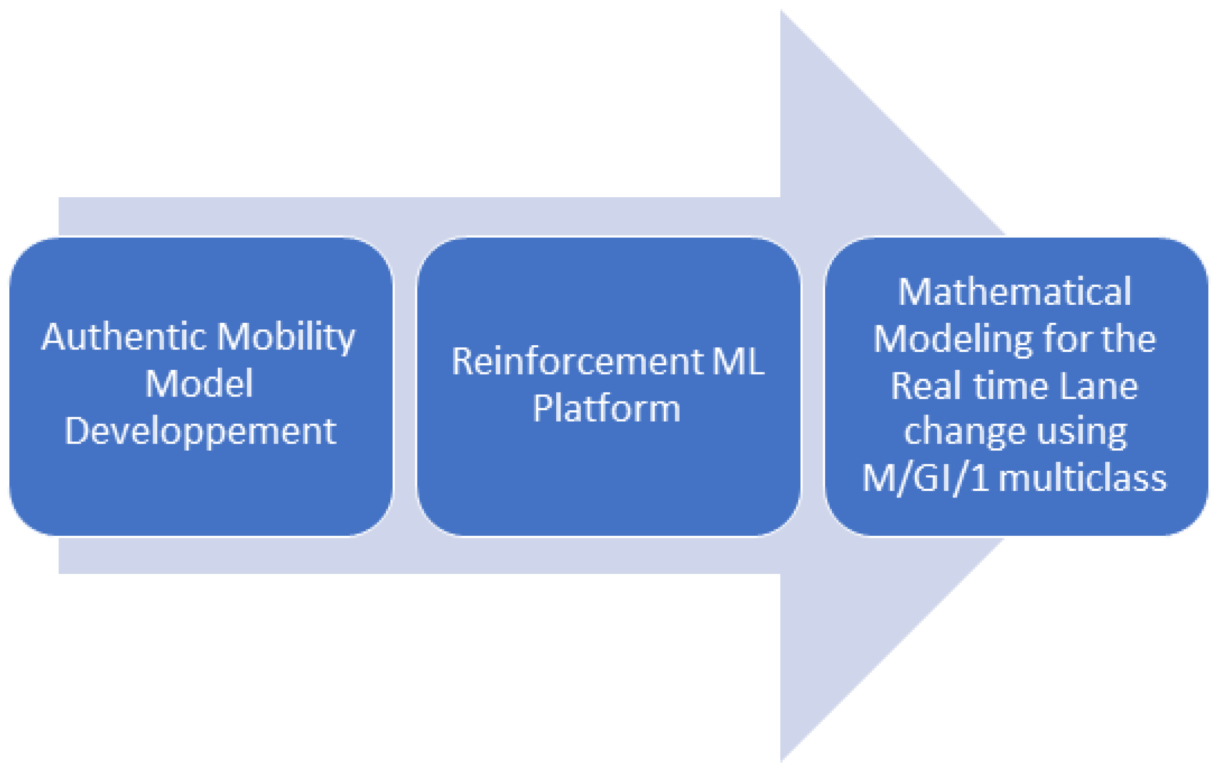
Our research study stands out of the literature for the following reasons (Figure 1):
- –
- Mobility models should simulate the real behavior of vehicular traffic, whilst it is critical to assess lane change decision modules for vehicle ad hoc networks. In fact, the vehicles distribution on highways is captured by the mobility model, which also affects vehicle trajectory. Performance results retrieved from simulations may not accurately reflect performance in an actual deployment in case a realistic mobility model is not used. Therefore, we adopt an authentic car-following mobility model to validate our lane change decision module in light of this understanding. The suggested module’s performance results demonstrate its advantages and demonstrate that it outperforms competing machine learning algorithms.
- –
- Research projects dealing with automatic lane switching adopt functions based on rule-based models; while these models may function well under typical common circumstances, they may be vulnerable to failure in the event of unforeseen conditions. Based on this knowledge, we develop a Reinforcement Federated Machine Learning based platform. The platform’s major goal is to train the vehicle agent to learn an automated lane change behavior so that it can lane shift intelligently in unforeseen situations. To calculate the total return, which is an accumulation of rewards across a lane shifting process, we specifically treat both state space and action space as continuous and construct a special format of Q-function approximator.
- –
- Lane change decision is a critical process that should be performed timely. Therefore, we perform a mathematical modelling of the downlink traffic at the Road Side Unit (RSU), using a M/GI/1 multiclass preemptive queue. The modelling is crucial to assess the real time feature of the lane change process.
3. Studied Lane Change Assistance Platform
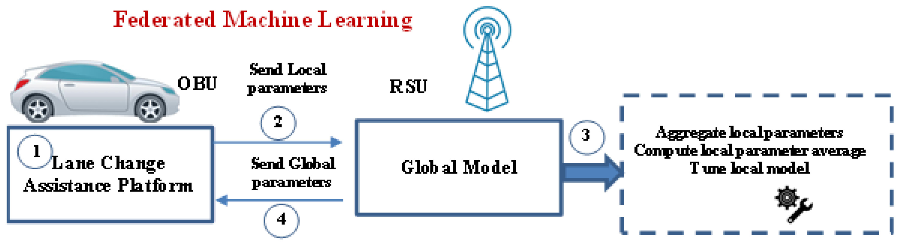
3.1. Global Federated Machine Learning Architecture
Figure 2 depicts the studied Lane Change Assistance (LCA) architecture that consists of two modules: local lane change assistance platform and global model provided by the federated machine learning. In fact, Federated Learning is implemented as a decentralized learning method where learners (vehicles OBUs) are randomly assigned to training datasets rather than having all the data centralized [50,51,52]. FL addresses the basic issues of privacy, ownership, and localization of data by taking the more general approach of “bringing the code to the data, instead of the data to the code”. Additionally, FL does not demand synchronization among OBUs, which are thought of as learners. Consequently, even when connectivity between OBUs and RSUs is lost, OBUs can still construct their local models and safely navigate; this capability is essential for highly dynamic and mission-critical V2V communication.
Within a limited number of communication iterations, FL enables the construction of learning models by sharing local models (a set of learning parameters) with a roadside unit. Since RSUs have a global view of the network, their centralizing ML processing procedures actually produce satisfactory results, but they also introduce latency and create a bottleneck in the cloud.
Local datasets cannot predict the global number of lane change collisions at the highway level due to the limited number of data observations that may be available to OBUs via V2V communications. Roadside equipment can therefore help collect samples via the network, but at the expense of higher data exchange costs. OBUs may also be reluctant to disclose their specific kinematic parameters and with an RSU and other OBUs for privacy purpose and for resource optimization; In fact, a significant data exchange could deplete the resources for vehicular communications. As a conclusion, a collaborative learning strategy that doesn’t rely on sharing individual data sets could address this restriction.
More specifically, our proposed platform operates as follows:
- –
- In a first stage, the OBUs apply a local lane change assistance platform which is extensively detailed in next subsection. In this context, OBUs exchange local ML model parameters with RSU.
- –
- At a second stage, a global model of a machine learning algorithm is maintained by an RSU. In fact, after receiving the local model parameters sent by each OBU, the RSU calculates model averaging across vehicles, fine-tunes these parameters, and then feeds back the global model to the OBUs. This will collaboratively and accurately detect lane change erroneous decisions and reduces collisions caused by lane changes.
Notably, the LCA architecture relies on various time scales: each OBU locally learns its model parameters over a short period, while the model averaging (global learning) occurs over a longer period.
The next subsection will bring the focus to the lane change assistance platform modules.
3.2. Local Lane Change Assistance Platform
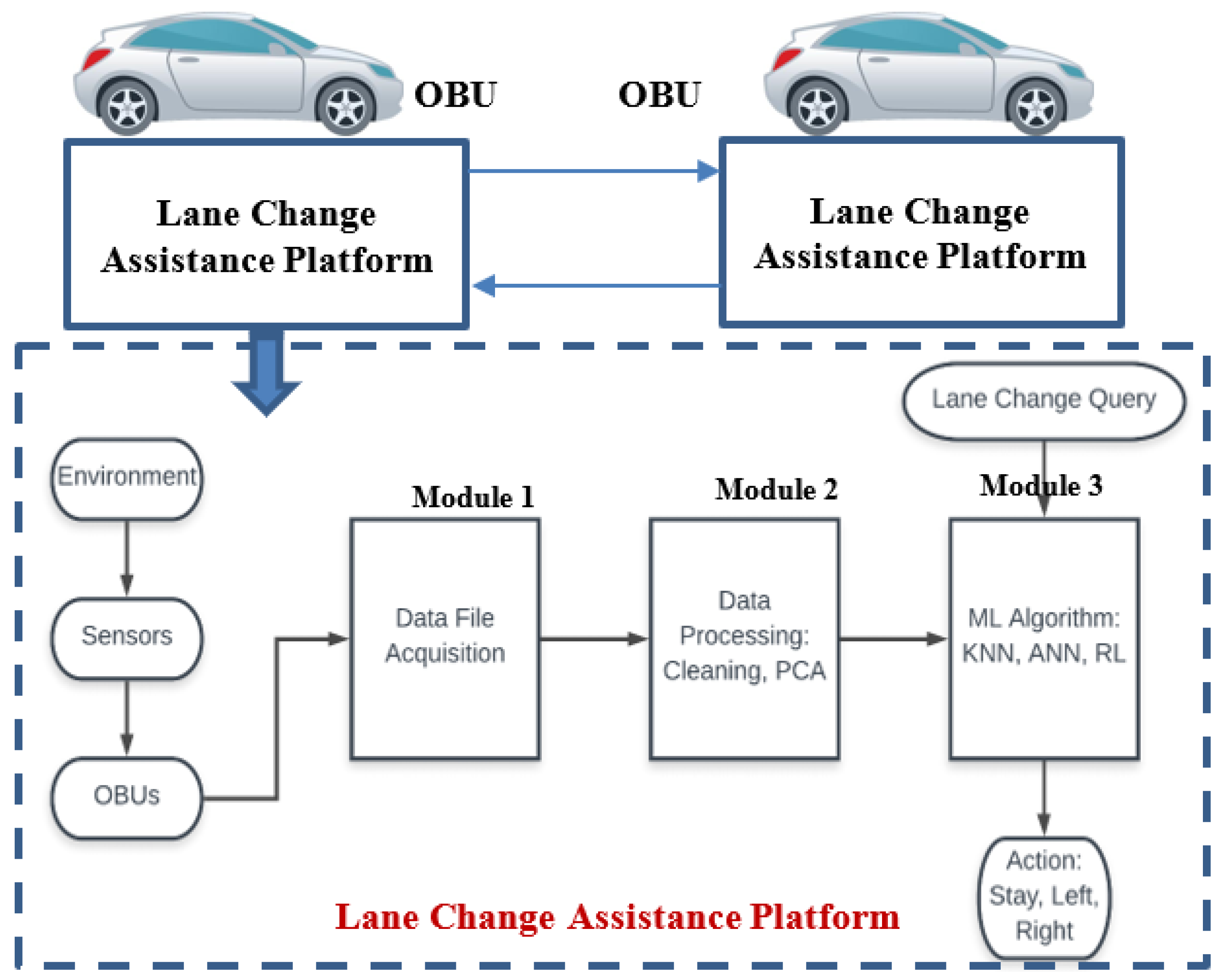
In order to process lane change queries, we designed a Lane Change Assistance platform illustrated by Figure 3. An ego vehicle (the vehicle under control) senses its environment and communicates with other cars using an OBU. Module 1 tackles the different types of data that are collected and stored in a data file. Next, module 2 cleans and processes the data as explained in the following paragraphs. When a lane change queryis raised, the processed data is fed into module 3. This module will take a real-time decision related to an action based on the input data. The action is: change lane to right, change lane to left, or stay in lane. The following paragraphs are devoted to the description of the three main building blocks of our platform:
- –
- Module 1: Data file acquisition
- –
- Module 2: Data processing
- –
- Module 3: Lane Change Decision Module
Module 1 is implemented with SUMO (Simulation of Urban Mobility) which is an open source, highly portable, microscopic and continuous traffic simulation package designed to handle large road networks. Module 2 and Module 3 are developed with Python. It is noteworthy that we adopted the TraCI python library (TRAffic Control Interface), that provides a seamless interaction between SUMO and python. TraCI is beneficial to link module 1 to the other modules.
3.2.1. Module 1: Data File Acquisition
Data was acquired using SUMO. At each time-step, kinematic data is collected form the “ego vehicle”, as well as from six surrounding vehicles in the current and adjacent lanes. The collected data file stores kinematic parameters retrieved by vehicle sensors and disseminated by OBUs. It consists of a table of 50 columns, where each column represents a single vehicle variable. The variables are detailed in the following list:
- –
- Time-step at which the data was collected;
- –
- Detected risk (−1 if no risk detected, else equal to the risky lane ID);
- –
- Ego vehicle variables: X position, Y position, lane ID, velocity, acceleration;
- –
- Neighboring vehicles variables: car ID, X position, Y position, lane ID, velocity, acceleration, distance to ego vehicle;
- –
- Action taken by ego (stay in lane, go left, or go right).
3.2.2. Module 2: Data Processing
Module 2 is a key component for data analytics. In our case, it performs the following three tasks:
- –
- Task1: Extract relevant data
- –
- Task 2: Fill NA (not assigned) values
- –
- Task 3: Reduce data dimension
Task 1: Extract relevant data The data file needed to be trimmed in the pretraining phase, as it contained some irrelevant information for a lane-change decision (e.g., the time step and car IDs). Therefore, we extracted the following data:
- –
- Y position, velocity, acceleration for the ego vehicle
- –
- Y position, velocity, acceleration, distance to ego for each of the neighboring vehicles
- –
- Action taken by ego vehicle (stay in lane, go left, or go right).
This step yields to a total of 28 variables. Twenty-seven represent the kinematic data that will be the input for the ML algorithm, and one variable (action) will be the desired output (label) of the algorithm.
Task 2: Fill NA values NA values occur in different scenarios:
- –
- At the highway entrance, where the ego vehicle does not have any followers in any lane.
- –
- At the highway exit, where the ego vehicle does not have any leaders.
- –
- At the right-most lane, where there are no right-side followers or leaders.
- –
- At the left-most lane, where there are no left-side followers or leaders.
In the first (resp. second) scenario, three virtual vehicles are added behind (resp. in front of) the ego vehicle in each of the 3 lanes of the highway. The virtual cars are 50 m behind (resp. ahead of) the ego vehicle, and have the same velocity and acceleration. In the third (resp. fourth) scenario, a virtual lane is added with an index of −1 (resp. 3), and two virtual cars are added in this lane, 50 m ahead and behind of the ego vehicle.
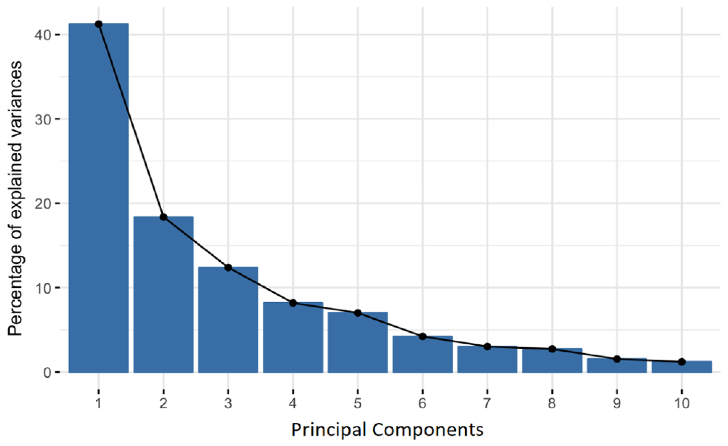
Task 3: Reduce data dimension with Principal Component Analysis Undoubtedly, accuracy degrades when the number of variables in a data collection is reduced. Nevertheless, smaller data sets can really be explored, analyzed, stored, and visualized more easily. For machine learning algorithms in particular, it makes data analysis much simpler and quicker. Principal Component Analysis (PCA) is a method for reducing the dimensionality of massive amounts of data while yet preserving as much information as possible [53]. The PCA method moves through the following steps in order to accomplish this goal (Figure 4): (1) Standardization (2) Calculation of covariance matrices (3) Computation of the principal components (4) principle component filtering and recasting of the data along the axis of the principle components (Figure 4).
(1) Standardization: In order for each continuous initial variable to contribute equally to the analysis, this phase standardizes the range of the variables. In fact, PCA is very sensitive to the initial variable variances. In other words, if there are significant variations between the initial variable ranges, the wide range variables will predominate over the short range variables, leading to biased results. Therefore, this issue can be avoided by translating data to comparable scales. This can be accomplished mathematically by dividing each value by the standard deviation after deducting the mean from each value.
(2) Covariance matrix computation: Due to their high correlation, variables sometimes contain redundant information. Therefore, it is of paramount importance to compute the covariance matrix in order to find these correlations. Checking for any relationships between variables is the goal of this stage. The covariance matrix, which holds the covariances related to all potential pairs of the initial variables, is a p × p symmetric matrix (where p is the number of variables). The two associated variables grow or decrease simultaneously when the covariance value is positive. One increases when the other declines (inversely linked) if the covariance value is negative.
(3) Compute principal components: The directions of the data with the greatest level of variance are represented by principal components: They are new variables created as a result of linear combining or mixing the initial variables. These combinations are carried out such that most of the information included in the original variables is compressed into the first components, which are the new uncorrelated variables (i.e., principal components). Since the eigen vectors of the covariance matrix are the directions of the axes that exhibit the highest variance (more information) and that we refer to as Principal Components, eigen vectors and eigen values are essential elements of the PCA process. The coefficients connected to eigen vectors, known as eigen values, are what determine how much variation is carried by each Principal Component. We obtain the principal components in order of importance by placing all of the eigen vectors in ascending order of their eigen values.
(4) Filter principal components and recast the data along the principal components’ axis: At this stage, we decide whether to preserve all of the significant components or to discard any that have low eigenvalues, and then we combine the remaining components to form the “Feature vector”. The data is then reoriented from the original axes to the ones indicated by the principal components using the feature vector created using the covariance matrix’s eigenvectors. To do this, we multiply the feature vector’s transposition by the original data set’s transposition.
PCA execution resulted in a reduction of the number of input variables from 27 to only 11, while preserving 90% of the information (variance).
3.2.3. Module 3: Lane Change Decision Module
Lane change decision is a critical process that should be taken carefully. We propose in this research work to devise the driver with the optimal decision, based on predictions conducted by one of the following three ML algorithms: (1) ANN, (2) KNN and (3) reinforcement Learning.
(1) Artificial Neural Network ANN: The training data set was divided in two sets, with (30%, 70%) proportions. Three different architectures were proposed and tested to find the one with the best accuracy.
- –
- Input layer: Within the input layer, we considered 11 input neurons with the ReLU activation function.
- –
- Hidden layers:
- *
- With the first architecture, we adopted 5 hidden layers with 20 neurons each, and a ReLu activation function
- *
- The second architecture relies on 5 hidden layers with 200 neurons each, and a ReLu activation function
- *
- With the third architecture, we adopted 12 hidden layers with 20 neurons each, and a ReLu activation function
- –
- Output Layer: Within the output layer, we considered 3 output neurons with the SoftMax activation function.Performance tests show that the first architecture exhibits the best prediction accuracy (0.89673).
(2) K-Nearest Neighbor KNN: In an effort to adjust the value of K parameter, we conducted a series of evaluations to assess the accuracy of multiple values of K. Therefore, we started by adopting 70% of the training data to train our algorithm, and 30% to test K accuracy. Highest accuracy is reached (0.908936) with K = 25.
(3) Reinforcement Learning RL: With this algorithm, no previous data points are collected. The vehicle starts driving, collecting data, and taking random lane change actions throughout the simulation. The collected data is then evaluated through a reward function defined as follows:
- *
- Positive reward equal to the distance driven with no collisions:
- *
- Negative reward:where:
- •
- , , and are negative rewards.
- •
- is the collision ratio sent by the RSU.
- •
- is the probability that the distance, separating two following vehicles, is less than the safety distance.
- •
- is the probability that an emergency brake occurs.
- •
- is the probability that a lane change takes place.
- *
- Total reward: R = + −1
Note that −1 is subtracted at each time step so that our agent learns to drive as fast as possible, while respecting appropriate safety conditions. A discount factor of = 0.95 was used to reduce the value of future rewards. After data collection and reward evaluation, we sampled 20% of these data points that had the highest 20% rewards. An ANN was trained using these data points, to be used in the next training episode to predict the best action (instead of taking random actions). The loop continues until the agent is fully trained.
It is noteworthy that during training phase, 10% of the performed lane change actions are predicted using a random policy instead of the ANN. This ensures that the environment exploration rate is high enough so that the neural network will not converge to some local minima.
4. End to End Delay Analysis
Lane change decision is a critical process that should be undertaken in a tight time window. Therefore, it is of paramount importance to evaluate the V2I communication delay. In this context, we perform an accurate mathematical modelling of the network data traffic at the RSU level. More specifically, we consider messages that fall into two classes.
- Class 1: Safety related message sent by the RSU; This message contains the collision ratio required for the RL utility function.
- Class 2: Global update sent by the RSU related to the OBU local update required for the federated machine learning.
It is obvious that class 1 has a higher priority that class 2.
This section tackles the delay computation using mathematical modelling based on a M/GI/1 multiclass. In fact, the total delay of a class-i request from a RSU to a vehicle-j, denoted as , consists of two parts:
- Queuing delay at the RSU,
- RSU-to-vehicle propagation delay,
Thus, we have
where is the set of vehicles in the scenario and is the maximum waiting time for a class-i request; the request will be considered as expired in case it is not processed by the RSU during .
The transmission delays at both the vehicle and the RSU side are neglected since these values are very small compared to the propagation delays.
4.1. Propagation Delay
The V2I propagation delay of a class-i request is calculated by
where is the distance separating the RSU from the vehicle-j, is the propagation speed.
4.2. Queuing Delay at the RSU Side
As previously mentioned, RSU tackles two types of messages: while the first deals with safety-related issues and has a high priority, the second carries the global update and has low priority. It should be noticed that the length of safety-related messages is variable and follows an exponential distribution. Conversely, the length of global update packets is constant.
At the RSU side, the service of a low priority request (i.e., global update) can be interrupted by the arrival of a high priority request (i.e., safety message). That is to say, the queuing model is a priority queuing with preemption. In this case, the waiting time of the high priority requests, denoted as , is not affected by the low priority requests, and is solely related to the arriving process and service process of requests of class-1. On the other hand, the waiting time of low priority requests, denoted as , is affected by high priority requests, with an additional waiting time due to the arrival and interruption from a high priority request.
Consequently, we model the message queuing at the RSU as a M/G/1 multiclass preemptive queue. The arriving process follows a Poisson process while the service time follows an exponential distribution. Moreover, the service times for different safety messages are independent and identically distributed. The arrival process and service time distributions for safety-related messages and global update messages are shown in Table 2.
We define the following variables:
- : the occupation rate of a class-i request;
- : the arrival rate of a class-i request;
- : the mean service time at the drone of a class-i request;
- : the mean waiting time in the queue of a class-i request;
- : the mean residual service time of a class-i request;
- : the mean sojourn time of a class-i request, note that ;
- : the average number of requests of class i waiting in the queue.
Thus, for the total incoming traffic at the RSU, we have the following:
4.2.1. Mean Waiting Time of High Priority Requests
The average waiting time can be expressed as follows:
where denote the number of high priority requests waiting in the queue.
According to Little’s law we have
Combining the two equations yields
Since we have
Equation (8) becomes
The sojourn time is then
4.2.2. Mean Waiting Time of Low Priority Requests
As explained before, the waiting time of low priority requests can be expressed as
The low priority packet has to first wait for the sum of the service times of all packets with the same priority or higher priority present in the queue plus the remaining service time of the packet in service. Thus,
On the other hand, the is related to all the higher priority requests arriving during its waiting time and service time. This leads to
Applying Little’s law gives:
We obtain
The mean sojourn time of a class-i customer follows from , yeilding
Since we have
Equation (15) finally becomes
5. Lane Change Assistance Platform Validation
5.1. Simulation Scenario
Conducting large-scale and extended trials on highway and free routes presents economic and logistical hurdles for testing and evaluating vehicular protocol implementations in real scenarios. As a result, simulation is a practical method for verifying networking protocols and a commonly used strategy for advancing the development of vehicular technology.
The appropriate description of vehicular mobility models is one of the key challenges encountered in vehicular simulations.
Without an authentic mobility model, VANETs performance results obtained from simulations may not be in phase with performance in a real highway deployment. In this context, we adopted which is an efficient car-following model, adapted for a single-lane, bi-directional straight road movement [54,55]. The model takes four input variables: the maximum velocity , the maximum acceleration a, the maximum deceleration b and the noise that introduces stochastic behavior to the model. It aims at
- Computing the safety speed of vehicle i, , required to maintain a safety distance from its leading vehicle.
- Determining the desired new speed of vehicle i, , which is equal to the current speed plus the increment determined by the uniform acceleration, upper bounded by the maximum safe speeds.
- Determining the actual speed of the vehicle i, , by adding some randomness, due to driver’s imperfection using the measure of a maximum percentage of the highest achievable speed increment . is a random variable uniformly distributed in [0, 1].
More specifically, the model updates the speeds of each interval according to the following equations:
(t + t) = min [, (t) + aΔt, (t + Δ t) ]
(t + Δ t) = max [0, (t + Δ t) −aΔt]
Krau model correctly reproduces the behavior of vehicles.
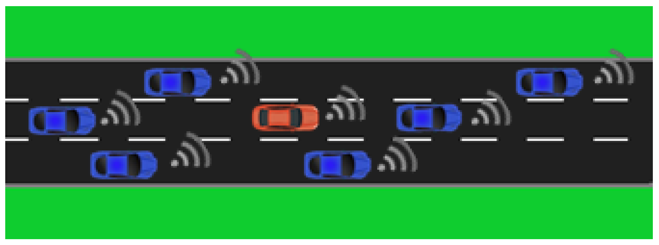
In order to validate the proposed model, we conducted extensive simulation batches. The simulation consists of 100 episodes. In each episode, the ego vehicle, with a maximal velocity of 100 km/h, tries to safely reach the end of a 3-lane highway of 2 km before the time runs out. Figure 5 illustrates the simulated highway where vehicles circulate towards the highway exit. The wireless infrastructure hosts multiple road side units exchanging messages. In this study, we that each RSU exchanges with OBUs information basically related to performance parameters.
5.2. Risk Modelling
A vehicle may encounter a collision risk, such as construction work, erroneous driver behavior or icy road. We modelled risk probability at one lane at a time. Whenever a risk is detected in a lane, the lane is tagged “risky” for a random distance, uniformly distributed on the highway, spanning between 30 and 200 m.
5.3. Performance Parameters
In order to evaluate the performance of the LCA platform, we measure several performance parameters, namely: Collision rate, emergency brakes frequency, sojourn time, and time driven in risky lanes.
5.4. Performance Analysis
The present subsection is dedicated for assessing the performance of the proposed platform, that adopts three ML algorithms: RL, KNN and ANN.
(1) Collision rate The main purpose behind our of LCA platform is to reduce fatalities induced by faulty lane change decision; hence collision rate is crucial for the performance analysis.
Table 3 shows a comparison between the three adopted ML algorithms in terms of collision rates. One can see that the reinforcement learning approach incur 15 collisions out of 100 episodes (15 car accidents where ego vehicle was involved), whereas both KNN and ANN agents lead to zero collisions.
In fact, many training batches were performed in order to reach an acceptable accuracy. As pointed out earlier, a high accuracy (0.908)was reached with K = 25. On the other hand, we oriented our efforts towards deriving the best architecture for the ANN algorithm that yields the best prediction accuracy (0.89). Performance tests show that the best accuracy was achieved with 5 hidden layers and 20 neurons. Therefore, we may conclude that ANN and KNN outperform the RL algorithm.
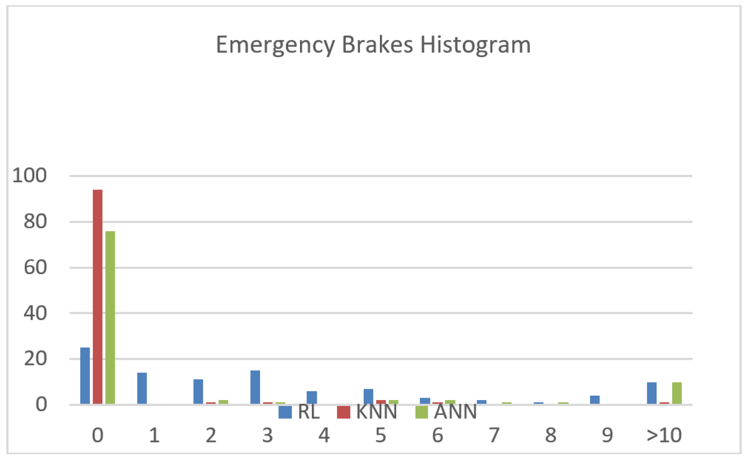
(2) Emergency brakes frequency A brake action is qualified by an emergency brake whenever the deceleration required to complete the brake falls below the minimum deceleration capacity of the vehicle. Figure 6 exhibits three histrograms related to the different adopted ML algorithms versus the episode number; the horizontal axis represents the number of emergency brakes number, and the vertical axis denotes the number of episodes (out of 100).
One can see that KNN outperforms other ML algorithms since more that 90 out of 100 episodes were completed with no emergency brakes at all. Table 2 depicts the average number of emergency brakes; Results point out that KNN induces the least number of emergency brakes. This is due to the fact that KNN exhibits the highest accuracy, as compared to the other algorithms. Therefore, we advise KNN to be applied in order to reduce emergency braking.
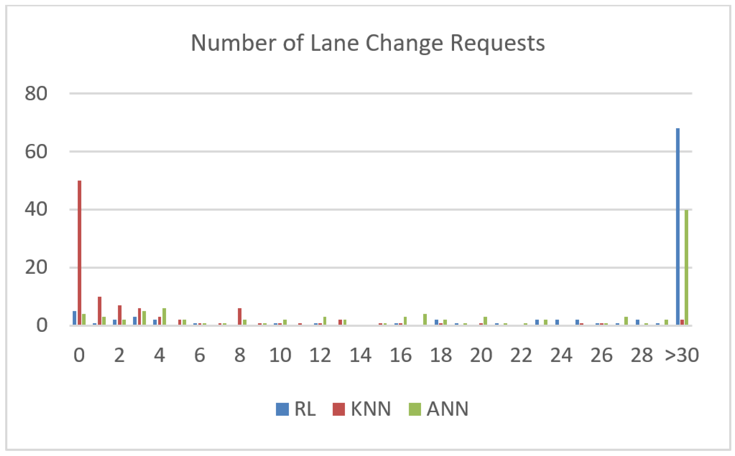
(3) Number of lane change requests Another important factor we need to take into consideration is the comfort of the vehicle passengers. A high number of lane changes induces a zigzag driving scheme can be annoying to the passengers as well as other drivers. Figure 7 exhibits the number of lane change (LC) requests issued by each of the ML algorithms, versus the episode number.
Table 3 depicts the average number of LC requests. It is clear that KNN achieves a relatively low number of lane change requests, followed by ANN, and finally RL. This points out that KNN tends towards reducing number of lane changes. The result is obvious due to the high accuracy of KNN that yields the lowest number of lane changes, as compared to the other algorithms. Therefore, KNN may be applied in order to reduce the annoying zigzag driving.
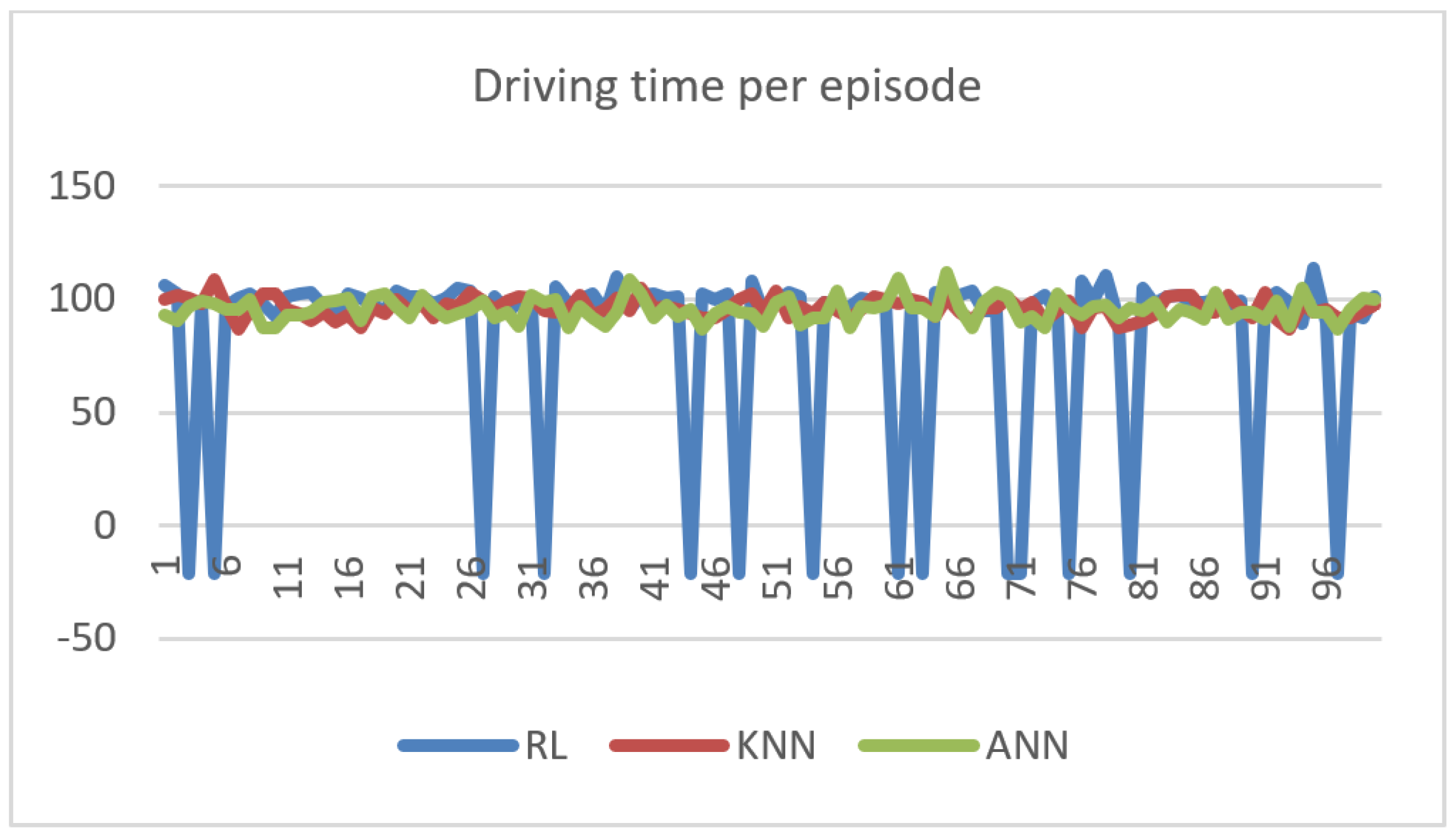
(4) Sojourn time Figure 8 illustrates the driving time versus episode number for each of the three ML algorithms. The negative blue peaks represent the episodes where the RL agent issues actions that result to car accidents (sojourn time = −1).
Table 4 shows a comparison between the average driving times of the ML algorithms. Results show that ANN leads to faster trips than with KNN, and both are faster than the RL agent. In fact, the result is expected: since ANN and KNN incur lower lane change, they tend towards keeping a high velocity; thus achieving low sojourn time.
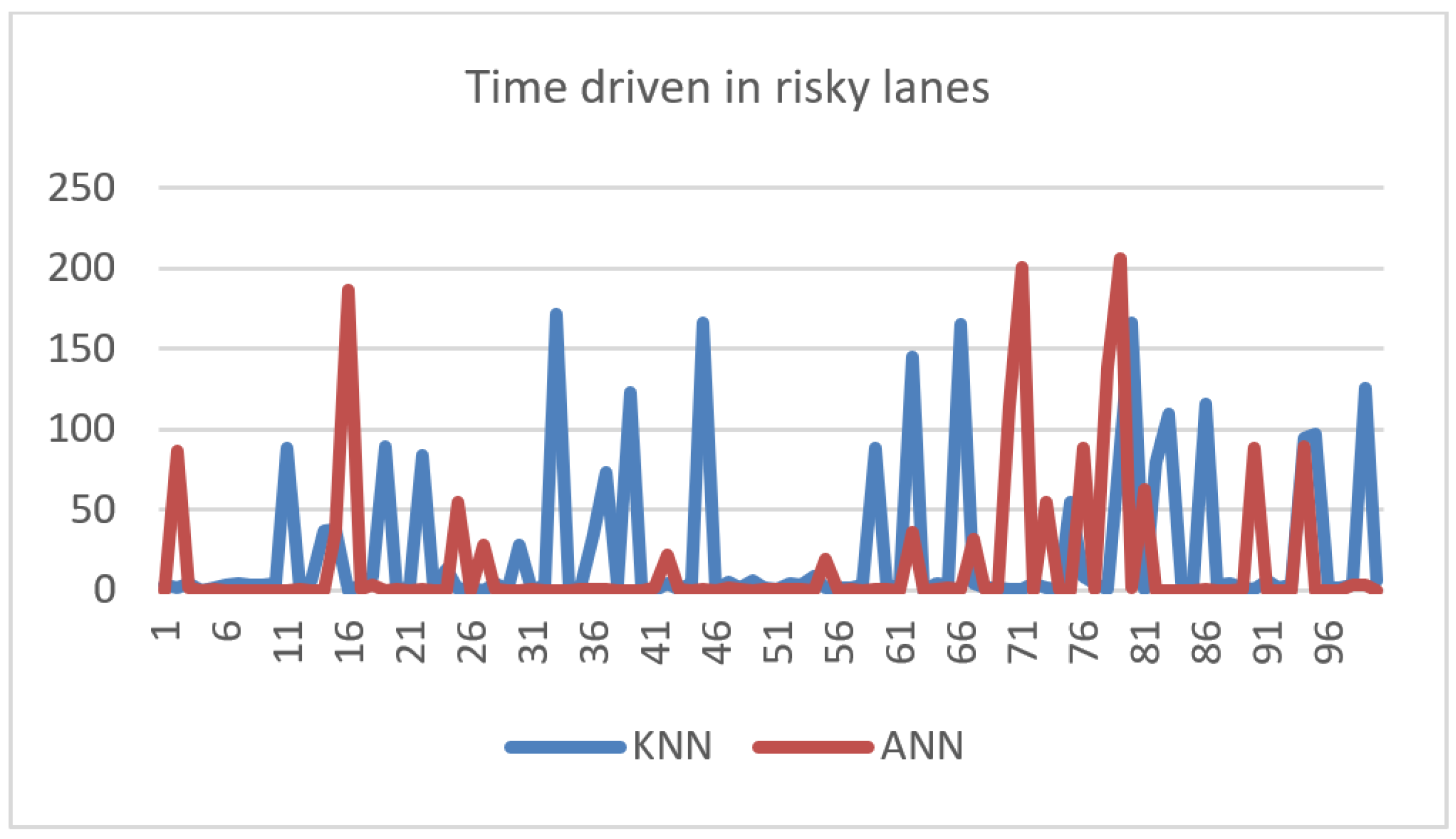
(5) Time driven in risky lanes Figure 9 illustrates the time driven in a risky lane versus episode number. The figure shows random peaks and fluctuations. To better understand the results, the average time was computed in Table 4.
We can see that this was the field where the ANN outperformed the KNN agent by a significant margin. This could be explained by the bias of the KNN agent towards staying in the lane. In fact, the KNN privileges reducing the lane-change request at the expense of continuing to drive in a risky lane for a higher time. Therefore, one can conclude that the ANN is advised when the driver prefers to avoid risky lanes.
(6) Waiting queue at the RSU Based on the mathematical modeling provided in Section 5, we computed the waiting average delay of the downlink traffic at the road side unit. The latter is responsible for processing global update messages and collision ratio dissemination, needed for the federated machine learning deployment. Results show that the average delay is bounded by 0.1 s which is quite acceptable to conduct lane change in real-time.
The following general conclusions can be drawn:
- The RL agent performs poorly. In fact, RL algorithms require relatively more training than regular algorithms, as they start learning from random data. Different tuning of reward and penalty points might also impact the speed of convergence of the algorithm.
- The KNN agent performs best out of the proposed algorithms, as it induces zero collision rate and the lowest emergency brake frequency. We note that this performance was a consequence of the bias of KNN towards staying in the same lane.
- The ANN agent presents relative satisfying performance, with zero collision rates. It is to be noted that ANN tends to cause higher emergency brakes due to the higher frequency of approved lane change requests. As a conclusion, the machine learning parameter models need to be dynamic and should adapt to the traffic fluctuation. This issue is under study in our future research work.
6. Conclusions
Erroneous lane change is a risky phenomenon that may lead to vehicle collisions. The present research paper provides a contribution to the development of Lane Change Assistance Platform based on machine learning algorithms. At a first step, we detailed the components of the proposed platform for lane change assistance: data file acquisition, data processing and lane change decision building blocks. At a second step, we deeply investigated data analytics process that is of paramount importance to data-driven decision making. Afterwards, we validated the platform through a detailed simulation and computed performance parameters.
In our perspectives, we intend to integrate Unmanned Aerial Vehicles (UAV), or drones, that will hover the vehicles. These drones will cooperate efficiently with the vehicles owing to their LoS (Line-of-Sight) links and dynamic deployment ability. More specifically, drones are equipped with dedicated sensors, high processing capabilities and communication devices, that enable them to undertake computations of the following parameters: vehicular density, collision rate computations and federated machine learning global model parameters. These computations will help to refine the reward function. Moreover, the cooperation with vehicles’ On-Board Units and infrastructures allows drones to improve infrastructure coverage and road active safety.
Funding
This work was supported by PHC-CEDRE Project 44390SA and Datawaves project, Labex Digicosme (project ANR11LABEX0045DIGICOSME) «Investissement d’Avenir» Idex ParisSaclay (ANR11IDEX000302). The author would like to thank Eng. Tarek Ghamrawi for his efforts to conduct simulations.
Data Availability Statement
Not applicable.
Conflicts of Interest
The authors declare no conflict of interest.
References
- Deng, L.; Ni, W.; Zhou, T.; Yu, Y.; Zhai, L. Analysis of Vehicle Assisted Lane Change System and Autonomous Lane Change Model. In Proceedings of the 2022 Fourth International Conference on Emerging Research in Electronics, Computer Science and Technology (ICERECT), Mandya, India, 26–27 December 2022; pp. 1–6. [Google Scholar] [CrossRef]
- Ranjan, A.; Sharma, S.; Goyal, H.R.; Kumar, K.C.N. Vehicle Collision Avoidance System During Lane Change using Internet-of-Things. In Proceedings of the 2023 International Conference on Intelligent Data Communication Technologies and Internet of Things (IDCIoT), Bengaluru, India, 5–7 January 2023; pp. 1–6. [Google Scholar] [CrossRef]
- Ouyang, K.; Wang, Y.; Li, Y.; Zhu, Y. Lane change decision planning for autonomous vehicles. In Proceedings of the IEEE Chinese Automation Congress (CAC), Shanghai, China, 6–8 November 2020; pp. 6277–6281. [Google Scholar] [CrossRef]
- Sun, M.; Chen, Z.; Li, H.; Fu, B. Cooperative Lane-Changing Strategy for Intelligent Vehicles. In Proceedings of the IEEE Chinese Control Conference (CCC), Shanghai, China, 26–28 July 2021; pp. 6022–6027. [Google Scholar] [CrossRef]
- Institute of Electrical and Electronics Engineers. IEEE Standard for Information Technology—Telecommunications and Information Exchange between Systems—Local and Metropolitan Area Networks—Specific Requirements Part 11: Wireless LAN Medium Access Control (MAC) and Physical Layer (PHY) Specifications; Institute of Electrical and Electronics Engineers: Piscataway, NJ, USA, 2007. [Google Scholar]
- ETSI 302665; Intelligent Transport Systems (ITS). Communications Architecture, 2010.
- Naja, R. Wireless Vehicular Networks for Car Collision Avoidance; Springer: Berlin/Heidelberg, Germany, 2013. [Google Scholar]
- Wan, F.; Li, M. Research on Coordinated Processing Scheme of Intelligent Transportation under Big Data Structure. In Proceedings of the IEEE 5th International Conference on Electromechanical Control Technology and Transportation (ICECTT), Nanchang, China, 15–17 May 2020; pp. 628–631. [Google Scholar] [CrossRef]
- Zhu, L.; Yu, F.R.; Wang, Y.; Ning, B.; Tang, T. Big Data Analytics in Intelligent Transportation Systems: A Survey. IEEE Trans. Intell. Transp. Syst. 2019, 20, 383–398. [Google Scholar] [CrossRef]
- Sliwa, B.; Adam, R.; Wietfeld, C. Client-Based Intelligence for Resource Efficient Vehicular Big Data Transfer in Future 6G Networks. IEEE Trans. Veh. Technol. 2021, 70, 5332–5346. [Google Scholar] [CrossRef]
- Alpaydin, E. Introduction to Machine Learning; MIT Press: Cambridge, MA, USA, 2014. [Google Scholar]
- Schmidhuber, J. Deep Learning in Neural Networks: An Overview. Neural Netw. 2015, 61, 85–117. [Google Scholar] [CrossRef] [PubMed] [Green Version]
- Jiang, C.; Zhang, H.; Ren, Y.; Han, Z.; Chen, K.; Hanzo, L. Machine Learning Paradigms for Next-Generation Wireless Networks. IEEE Wirel. Commun. 2017, 24, 98–105. [Google Scholar] [CrossRef] [Green Version]
- Lv, Y.; Duan, Y.; Kang, W.; Li, Z.; Wang, F. Traffic Flow Prediction With Big Data: A Deep Learning Approach. IEEE Trans. Intell. Transp. Syst. 2015, 16, 865–873. [Google Scholar] [CrossRef]
- Ye, H.; Li, G.Y.; Juang, B.H.F. Deep Reinforcement Learning Based Resource Allocation for V2V Communications. IEEE Trans. Veh. Technol. 2019, 68, 3163–3173. [Google Scholar] [CrossRef] [Green Version]
- Khan Tayyaba, S.; Khattak, H.A.; Almogren, A.; Shah, M.A.; Ud Din, I.; Alkhalifa, I.; Guizani, M. 5G Vehicular Network Resource Management for Improving Radio Access Through Machine Learning. IEEE Access 2020, 8, 6792–6800. [Google Scholar] [CrossRef]
- Afify, A.A.; Mokhtar, B. Machine Learning-based Services Provisioning for Intelligent Internet of Vehicles. In Proceedings of the 2021 IEEE 7th World Forum on Internet of Things (WF-IoT), New Orleans, LA, USA, 14 June–31 July 2021; pp. 51–54. [Google Scholar] [CrossRef]
- Aljeri, N.; Boukerche, A. A Novel Online Machine Learning Based RSU Prediction Scheme for Intelligent Vehicular Networks. In Proceedings of the 2019 IEEE/ACS 16th International Conference on Computer Systems and Applications (AICCSA), Abu Dhabi, United Arab Emirates, 3–7 November 2019; pp. 1–8. [Google Scholar] [CrossRef]
- Wang, X.; Liu, J.; Qiu, T.; Mu, C.; Chen, C.; Zhou, P. A Real-Time Collision Prediction Mechanism With Deep Learning for Intelligent Transportation System. IEEE Trans. Veh. Technol. 2020, 69, 9497–9508. [Google Scholar] [CrossRef]
- Zheng, Q.; Zheng, K.; Zhang, H.; Leung, V. Delay-optimal virtualized radio resource scheduling in software-defined vehicular networks via stochastic learning. IEEE Trans. Veh. Technol. 2016, 65, 7857–7867. [Google Scholar] [CrossRef]
- Ahmed, K. Modeling Drivers’ Acceleration and Lane Changing Behavior. Ph.D. Thesis, Massachusetts Institute of Technology, Cambridge, MA, USA, 2005. [Google Scholar]
- Julian, E.; Damerow, F. Complex Lane Change Behavior in the Foresighted Driver Model. In Proceedings of the 2015 IEEE 18th International Conference on Intelligent Transportation Systems, Gran Canaria, Spain, 15–18 September 2015; pp. 1747–1754. [Google Scholar]
- Nilsson, J.; Silvlin, J.; Brännström, M.; Coelingh, E.; Fredriksson, J. If, When, and How to Perform Lane Change Maneuvers on Highways. IEEE Intell. Transp. Syst. Mag. 2016, 8, 68–78. [Google Scholar] [CrossRef]
- Ulbrich, S.; Maurer, M. Towards Tactical Lane Change Behavior Planning for Automated Vehicles. In Proceedings of the 2015 IEEE 18th International Conference on Intelligent Transportation Systems, Gran Canaria, Spain, 15–18 September 2015; pp. 989–995. [Google Scholar] [CrossRef] [Green Version]
- Sunberg, Z.; Ho, C.; Kochenderfer, M. The value of inferring the internal state of traffic participants for autonomous freeway driving. In Proceedings of the 2017 American Control Conference (ACC), Seattle, WA, USA, 24–26 May 2017; pp. 3004–3010. [Google Scholar]
- Treiber, M.; Hennecke, A.; Helbing, D. Congested Traffic States in Empirical Observations and Microscopic Simulations. Phys. Rev. E 2000, 62, 1805–1824. [Google Scholar] [CrossRef] [Green Version]
- Kesting, A.; Treiber, M.; Helbing, D. General Lane-Changing Model MOBIL for Car-Following Models. Transp. Res. Rec. 2007, 1999, 86–94. [Google Scholar] [CrossRef] [Green Version]
- Hoel, C.; Wolff, K.; Laine, L. Automated Speed and Lane Change Decision Making using Deep Reinforcement Learning. In Proceedings of the 2018 21st International Conference on Intelligent Transportation Systems (ITSC), Maui, HI, USA, 4–7 November 2018. [Google Scholar]
- Zhou, J.; Zheng, H.; Wang, J.; Wang, Y.; Zhang, B.; Shao, Q. Multiobjective Optimization of Lane-Changing Strategy for Intelligent Vehicles in Complex Driving Environments. IEEE Trans. Veh. Technol. 2020, 69, 1291–1308. [Google Scholar] [CrossRef]
- Hegde, B.; Bouroche, M. Design of AI-based lane changing modules in connected and autonomous vehicles: A survey. In Proceedings of the 2022 Workshop Agents in Traffic and Transportation, Vienna, Austria, 25 July 2022. [Google Scholar]
- Bermejo, S.; Cabestany, J. Adaptive soft k-nearest-neighbour classifiers. Pattern Recognit. 2000, 33, 1999–2005. [Google Scholar] [CrossRef]
- McCulloch, W.; Pitts, W.A. Alogical calculus of the ideas immanent in nervous activity. Bull. Math. Biophys. 1943, 5, 115–133. [Google Scholar] [CrossRef]
- Rosenblatt, F. Principles of Neurodynamics: Perceptions and the Theory of Brain Mechanism; Spartan Books: Washington, DC, USA, 1961; Volume 5. [Google Scholar]
- Sutton, R.; Barto, A. Reinforcement Learning: An Introduction; MIT Press: Cambridge, MA, USA, 2017. [Google Scholar]
- Tong, W.; Hussain, A.; Bo, W.; Maharjan, S. Artificial Intelligence for Vehicle-to-Everything: A Survey. IEEE Access 2019, 7, 10823–10843. [Google Scholar] [CrossRef]
- Veres, M.; Moussa, M.A. Deep Learning for Intelligent Transportation Systems: A Survey of Emerging Trends. IEEE Trans. Intell. Transp. Syst. 2020, 21, 3152–3168. [Google Scholar] [CrossRef]
- Dong, J.; Chen, S.; Li, Y.; Du, R.; Steinfeld, A.; Labi, S. Space-weighted information fusion using deep reinforcement learning: The context of tactical control of lane-changing autonomous vehicles and connectivity range assessment. Transp. Res. Part C Emerg. Technol. 2021, 128, 103192. [Google Scholar] [CrossRef]
- Chen, S.; Dong, J.; Ha, P.; Li, Y.; Labi, S. Graph neural network and reinforcement learning for multi-agent cooperative control of connected autonomous vehicles. Comput.-Aided Civ. Infrastruct. Eng. 2021, 36, 838–857. [Google Scholar] [CrossRef]
- Hwang, S.; Lee, K.; Jeon, H.; Kum, D. Autonomous Vehicle Cut-In Algorithm for Lane-Merging Scenarios via Policy-Based Reinforcement Learning Nested within Finite-State Machine. IEEE Trans. Intell. Transp. Syst. 2022, 23, 17594–17606. [Google Scholar] [CrossRef]
- Mnih, V.; Kavukcuoglu, K.; Silver, D.; Rusu, A.; Veness, J.; Bellemare, M.; Graves, A.; Riedmiller, M.; Fidjeland, A.; Ostrovski, G.; et al. Human-level control through deep reinforcement learning. Nature 2015, 518, 529–533. [Google Scholar] [CrossRef] [PubMed]
- Liao, X.; Zhao, X.; Wang, Z.; Han, K.; Tiwari, P.; Barth, M.J.; Wu, G. Game Theory-Based Ramp Merging for Mixed Traffic with Unity-SUMO Co-Simulation. IEEE Trans. Syst. Man Cybern. Syst. 2022, 52, 5746–5757. [Google Scholar] [CrossRef]
- Dong, J.; Chen, S.; Li, Y.; Ha, P.Y.J.; Du, R.; Steinfeld, A.; Labi, S. Spatio-weighted information fusion and DRL-based control for connected autonomous vehicles. In Proceedings of the 2020 IEEE 23rd International Conference on Intelligent Transportation Systems (ITSC), Rhodes, Greece, 20–23 September 2020; pp. 1–6. [Google Scholar] [CrossRef]
- Yu, C.; Wang, X.; Xu, X.; Zhang, M.; Ge, H.; Ren, J.; Sun, L.; Chen, B.; Tan, G. Distributed Multiagent Coordinated Learning for Autonomous Driving in Highways Based on Dynamic Coordination Graphs. IEEE Trans. Intell. Transp. Syst. 2020, 21, 735–748. [Google Scholar] [CrossRef]
- Häfner, B.; Bajpai, V.; Ott, J.; Schmitt, G.A. A Survey on Cooperative Architectures and Maneuvers for Connected and Automated Vehicles. IEEE Commun. Surv. Tutor. 2022, 24, 380–403. [Google Scholar] [CrossRef]
- Yang, Y.; Luo, R.; Li, M.; Zhou, M.; Zhang, W.; Wang, J. Mean Field Multi-Agent Reinforcement Learning. In Proceedings of the 35th International Conference on Machine Learning, Stockholm, Sweden, 10–15 July 2018; Volume 80, pp. 5571–5580. [Google Scholar]
- Shi, P.; Yan, B. A Survey on Intelligent Control for Multiagent Systems. IEEE Trans. Syst. Man Cybern. Syst. 2021, 51, 161–175. [Google Scholar] [CrossRef]
- Garg, M.; Johnston, C.; Bouroche, M. Can Connected Autonomous Vehicles really improve mixed traffic efficiency in realistic scenarios? In Proceedings of the 2021 IEEE International Intelligent Transportation Systems Conference (ITSC), Indianapolis, IN, USA, 19–22 September 2021; pp. 2011–2018. [Google Scholar] [CrossRef]
- Zhou, W.; Chen, D.; Yan, J.; Li, Z.; Yin, H.; Ge, W. Multi-agent reinforcement learning for cooperative lane changing of connected and autonomous vehicles in mixed traffic. Auton. Intell. Syst. 2022, 2, 5. [Google Scholar] [CrossRef]
- Ha, Y.J.; Chen, S.; Dong, J.; Du, R.; Li, Y.; Labi, S. Leveraging the Capabilities of Connected and Autonomous Vehicles and Multi-Agent Reinforcement Learning to Mitigate Highway Bottleneck Congestion. arXiv 2020, arXiv:2010.05436. [Google Scholar]
- Zeng, T.; Semiari, O.; Chen, M.; Saad, W.; Bennis, M. Federated Learning on the Road Autonomous Controller Design for Connected and Autonomous Vehicles. IEEE Trans. Wirel. Commun. 2022, 21, 10407–10423. [Google Scholar] [CrossRef]
- Konecny, J.; McMahan, H.B.; Ramage, D.; Richtarik, P. Federated Optimization: Distributed Machine Learning for On-Device Intelligence. arXiv 2016, arXiv:1610.02527. [Google Scholar]
- Samarakoon, S.; Bennis, M.; Saad, W.; Debbah, M. Federated Learning for Ultra-Reliable Low-Latency V2V Communications. In Proceedings of the 2018 IEEE Global Communications Conference (GLOBECOM), Abu Dhabi, United Arab Emirates, 9–13 December 2018. [Google Scholar]
- Giordani, P. Principal Component Analysis. In Encyclopedia of Social Network Analysis and Mining; Alhajj, R., Rokne, J., Eds.; Springer: New York, NY, USA, 2018; pp. 1831–1844. [Google Scholar] [CrossRef]
- Davies, V. Evaluating Mobility Models within an Ad Hoc Network. Master’s Thesis, Colorado School of Mines, Golden, CO, USA, 2000. [Google Scholar]
- Fiore, M.; Harri, J.; Filali, F.; Bonnet, C. Understanding Vehicular Mobility in Network Simulation. In Proceedings of the IEEE International Conference on Mobile Adhoc and Sensor Systems, Pisa, Italy, 8–11 October 2007; pp. 1–6. [Google Scholar] [CrossRef]
Figure 1.
Proposed research work process.

Figure 2.
Proposed Federated Machine Learning based architecture.

Figure 3.
Lane Change Assistance Platform.

Figure 4.
PCA Principal Components.

Figure 5.
Simulated Highway.

Figure 6.
Emergency Brakes Histogram.

Figure 7.
Lane Change Requests Histogram versus Episode Number.

Figure 8.
Driving Time (s) versus Episode Number.

Figure 9.
Time Driven in Risky Lanes (s) versus Episode Number.

Table 2.
The arrival process and service time distributions.
| Arrival Process | Service Time Distribution | |
|---|---|---|
| Safety Message | Poisson | Exponential |
| Global update message | Uniform | Constant |
Table 3.
Performance Parameters.
| Parameters | RL | KNN | ANN |
|---|---|---|---|
| Collision rate | 15 | 0 | 0 |
| Average number of emergency brakes | 3.89 | 0.45 | 2.88 |
| Average number of lane change requests per episode | 38.27 | 3.91 | 31.66 |
| Average sojourn time | 100.0259 | 96.294 | 95.607 |
Table 4.
Average Time Driven (s) in Risky Lanes versus Episode Number.
| KNN | ANN |
|---|---|
| 24.87 | 15.91 |
Disclaimer/Publisher’s Note: The statements, opinions and data contained in all publications are solely those of the individual author(s) and contributor(s) and not of MDPI and/or the editor(s). MDPI and/or the editor(s) disclaim responsibility for any injury to people or property resulting from any ideas, methods, instructions or products referred to in the content. |
© 2023 by the author. Licensee MDPI, Basel, Switzerland. This article is an open access article distributed under the terms and conditions of the Creative Commons Attribution (CC BY) license (https://creativecommons.org/licenses/by/4.0/).
Share and Cite
MDPI and ACS Style
Naja, R. Safe Data-Driven Lane Change Decision Using Machine Learning in Vehicular Networks. J. Sens. Actuator Netw. 2023, 12, 59. https://doi.org/10.3390/jsan12040059
AMA Style
Naja R. Safe Data-Driven Lane Change Decision Using Machine Learning in Vehicular Networks. Journal of Sensor and Actuator Networks. 2023; 12(4):59. https://doi.org/10.3390/jsan12040059
Chicago/Turabian StyleNaja, Rola. 2023. "Safe Data-Driven Lane Change Decision Using Machine Learning in Vehicular Networks" Journal of Sensor and Actuator Networks 12, no. 4: 59. https://doi.org/10.3390/jsan12040059
Note that from the first issue of 2016, this journal uses article numbers instead of page numbers. See further details here.