
Improved Performance on Wireless Sensors Network Using Multi-Channel Clustering Hierarchy
Abstract
:1. Introduction
- -
- Point-to-point Topology,
- -
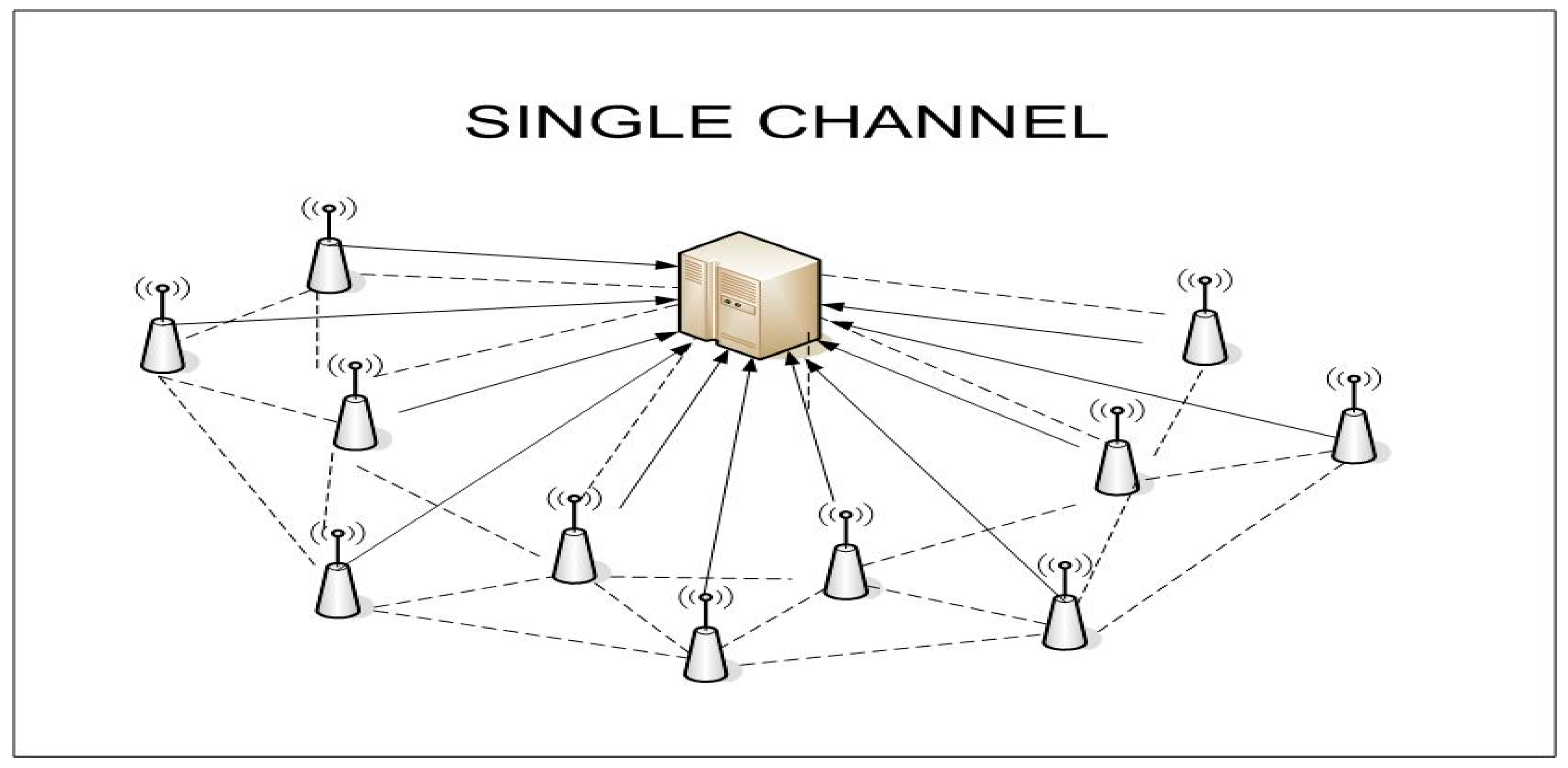
- Star Topology,
- -
- Mesh Topology,
- -
- Hybrid Technology,
- -
- Tree Topology.
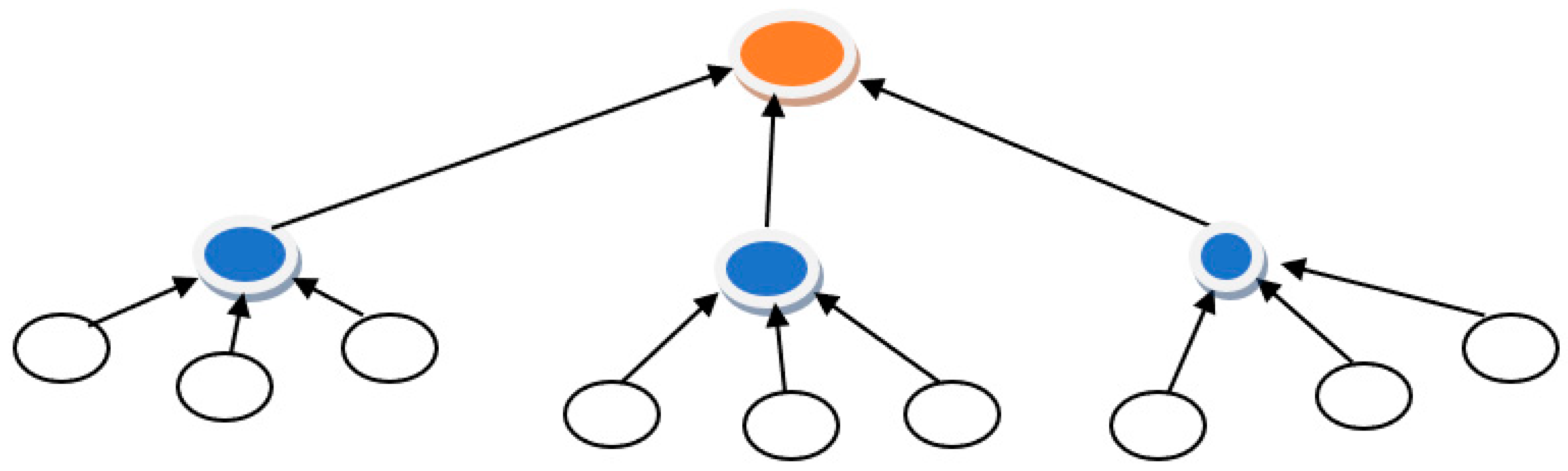
Clustering on Wireless Sensor Network
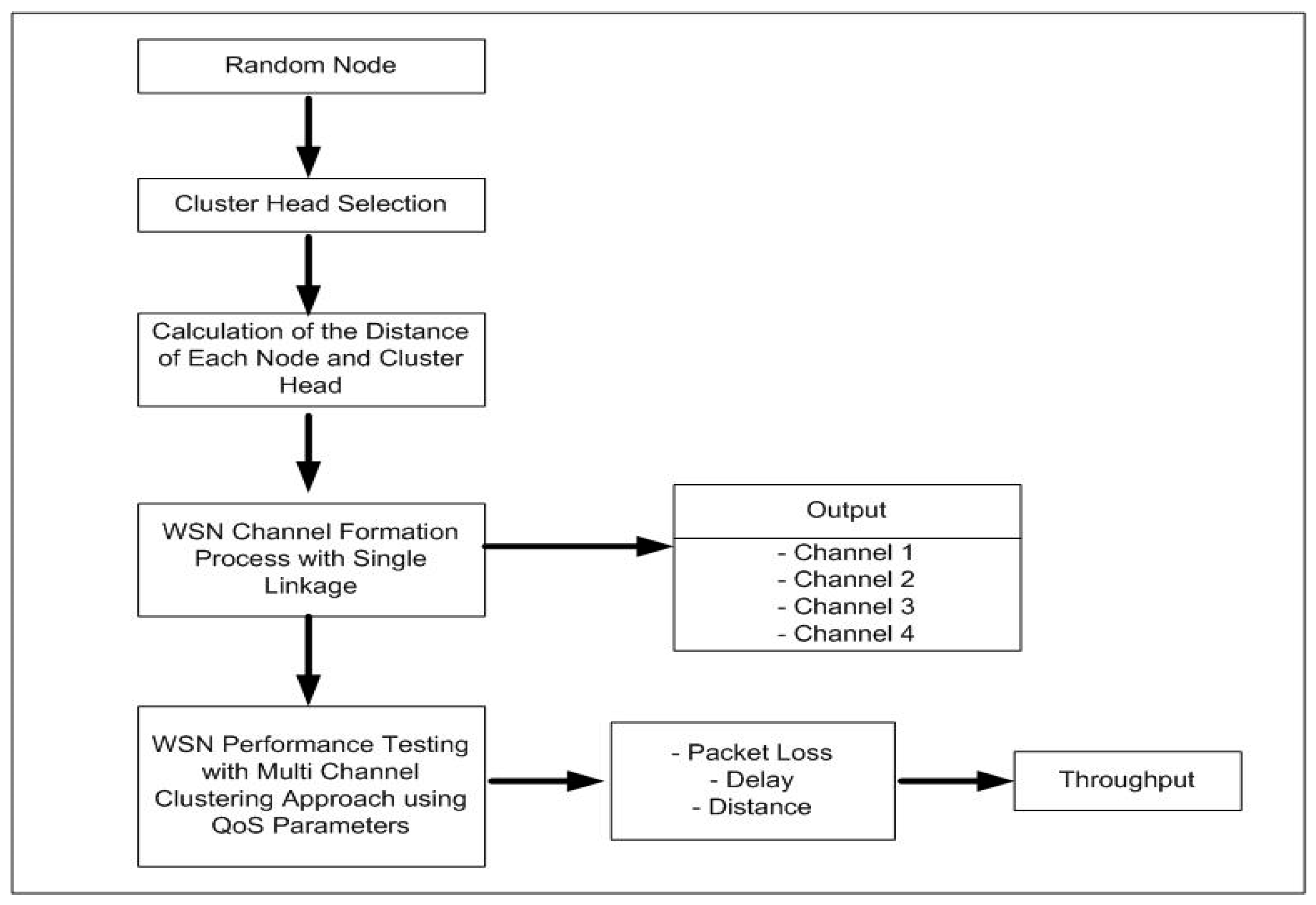
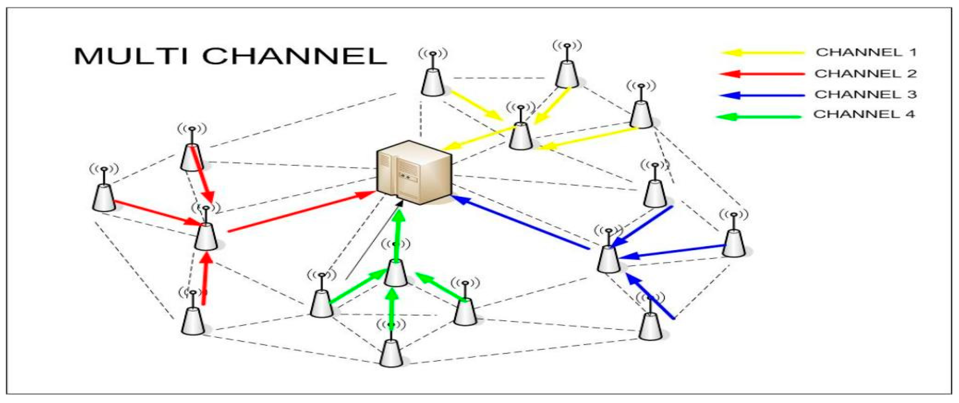
2. Multi-Channel Clustering Hierarchy (MCCH)
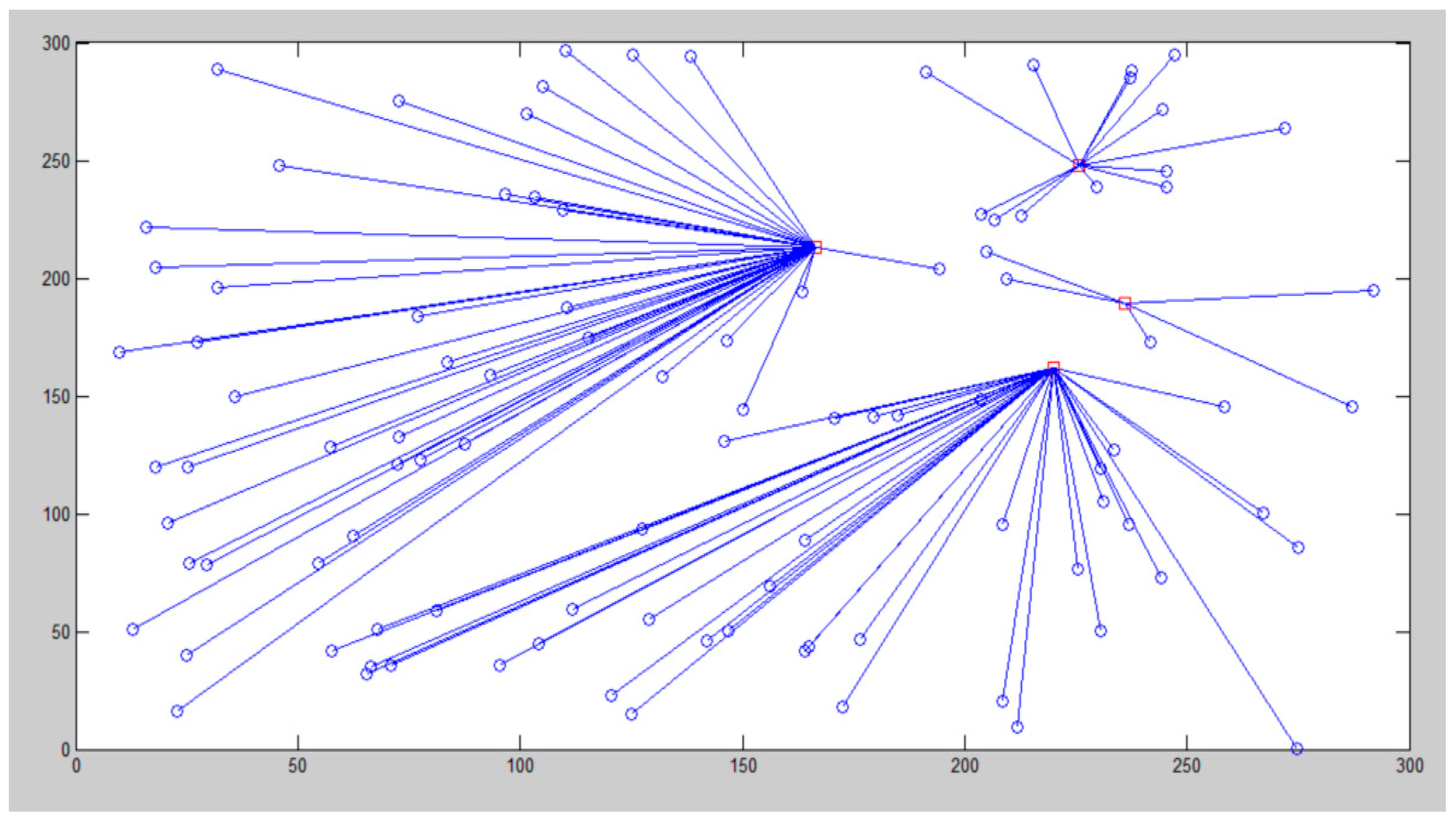
2.1. Cluster Head Selection
- Several sessions depending on the desired amount of CH and the period of observation are carried out.
- The CH position for each node for one session is ensured.
- The position of CH becomes unstable or alternates so that a Cluster has a dynamic formation or changes every session.
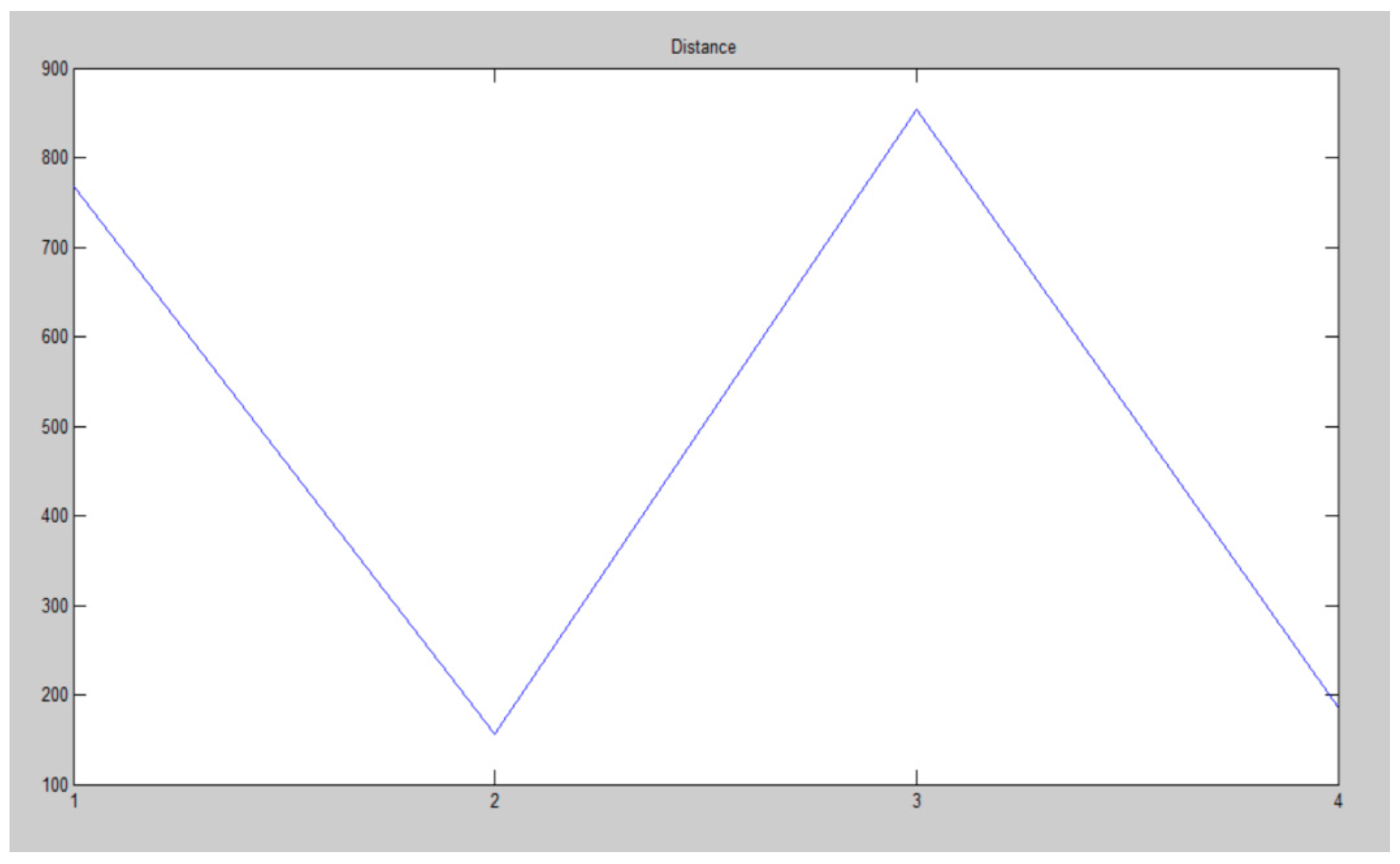
2.2. Calculation of the Distance of Each Node and Cluster Head
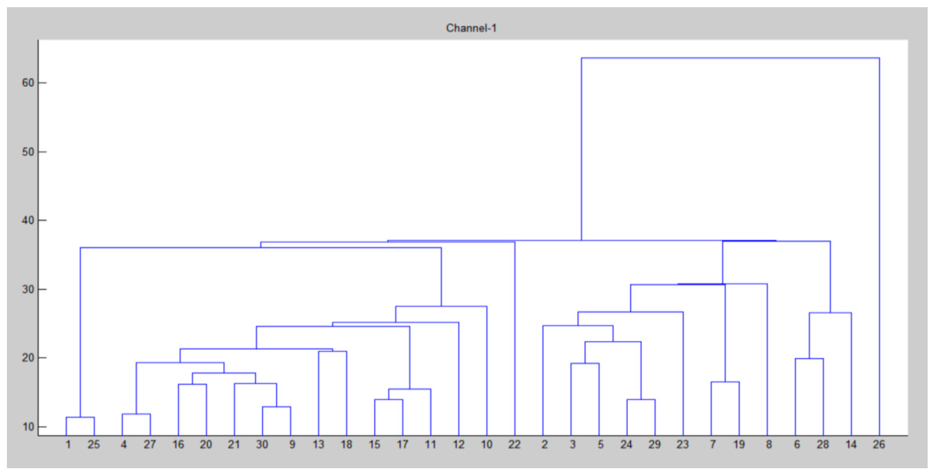
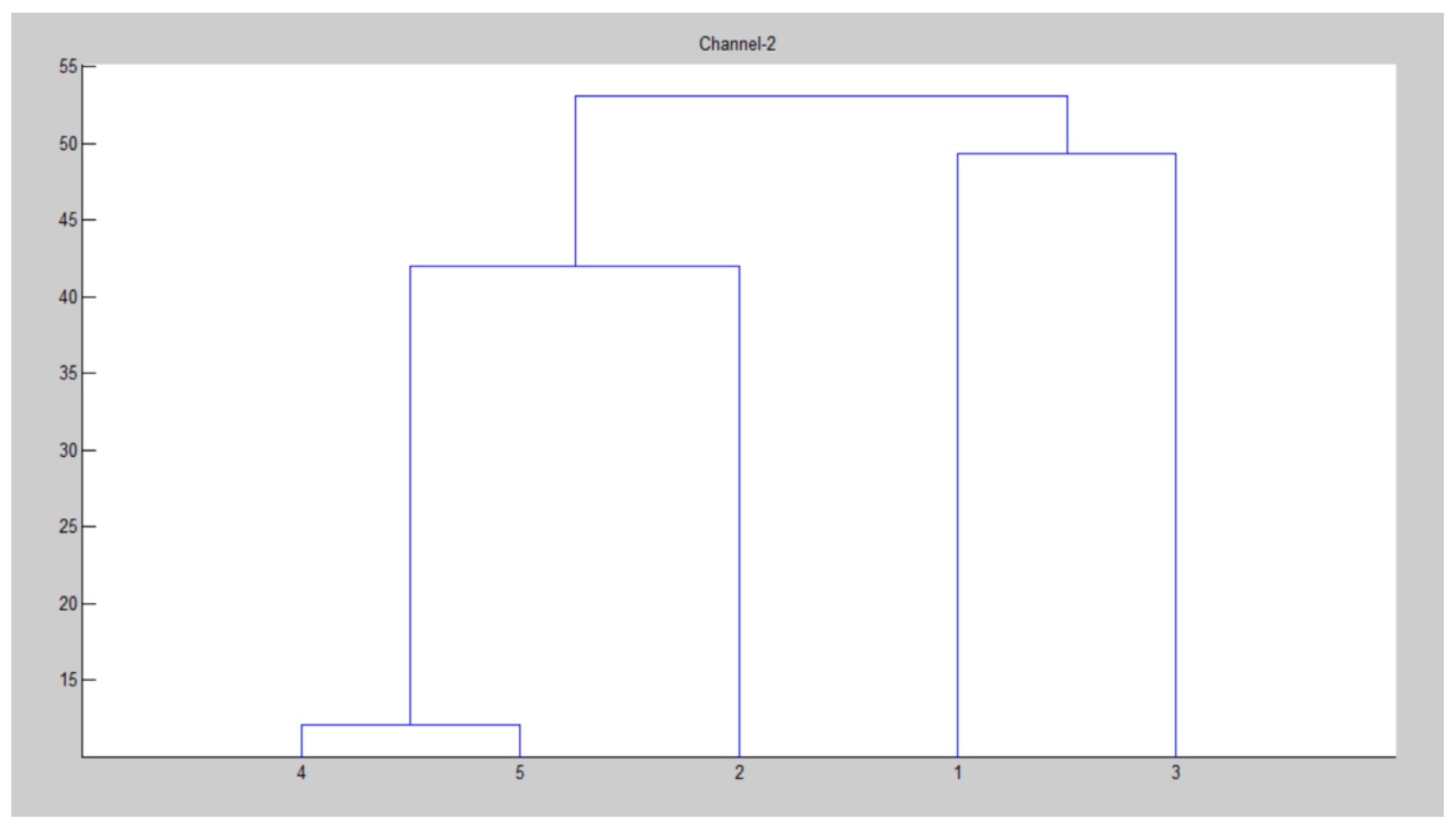
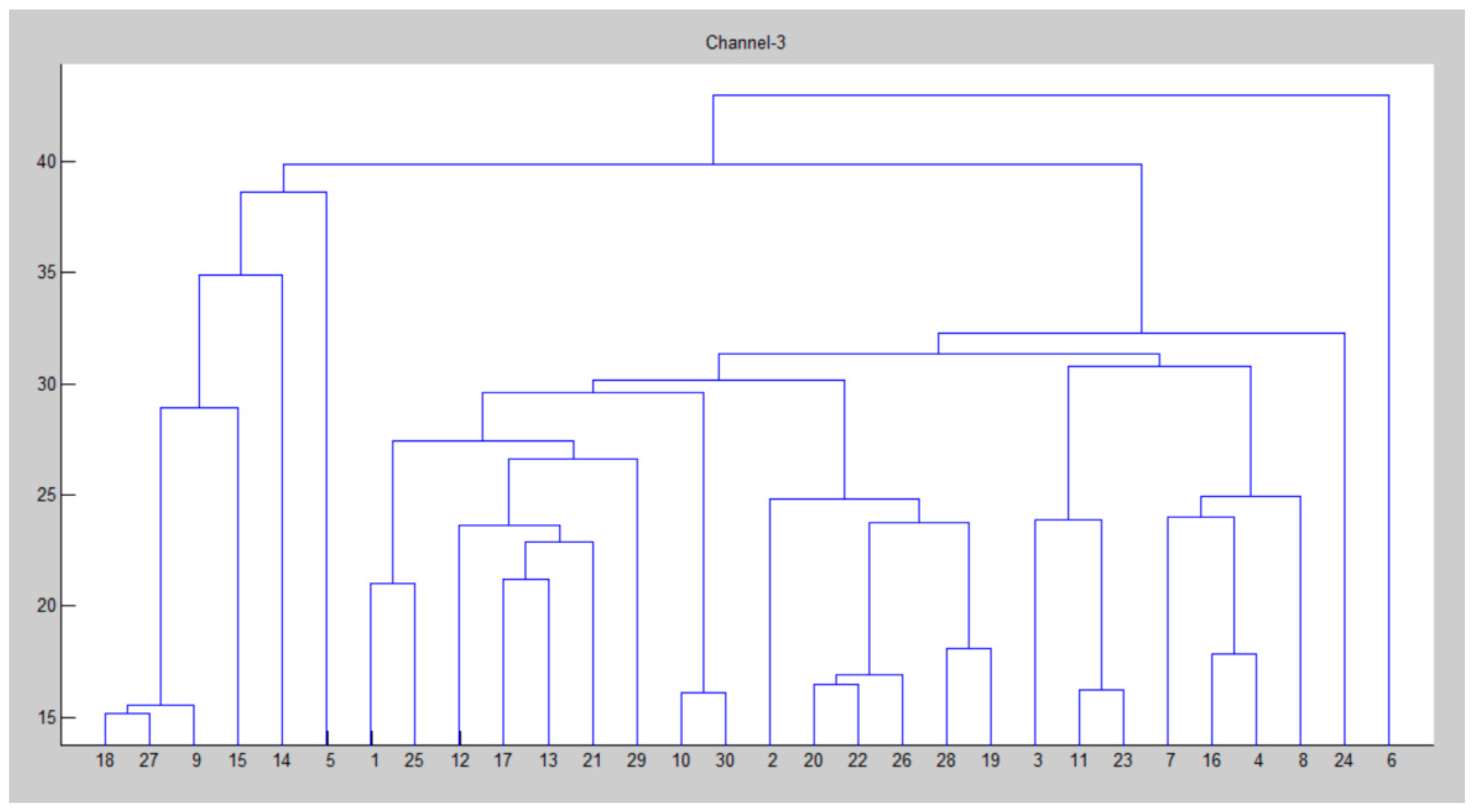
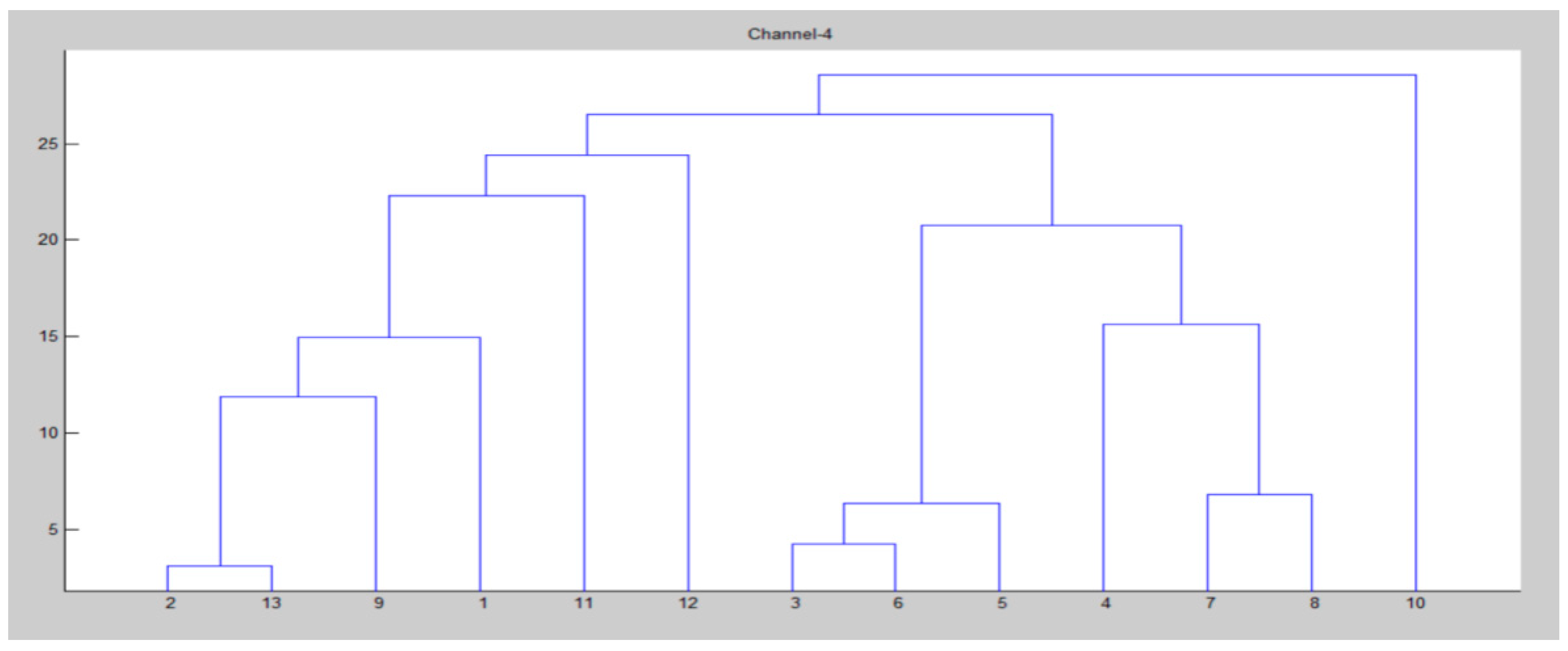
2.3. The Process of Forming a WSN Channel
- contains a single entity and a symmetric matrix of the distance (similarities)
- Find the distance matrix for the closest (most similar) cluster pair. For example, the distance between clusters U and V that is most similar is d u v.
- Merge the newly formed cluster U and V cluster labels with (UV). Then, update the entries in the distance matrix in the following way:
- Delete rows and columns corresponding to clusters U and V.
- Add rows and columns giving the distances between the cluster (UV) and the remaining clusters.
- Repeat steps 2 and 3 (N − 1) times. All objects will be in a single cluster after the algorithm ends. Note the identity of the merged cluster and the level (distance or similarity) at which the merger occurs.
3. Measurement of WSN Performance Using QoS Parameters
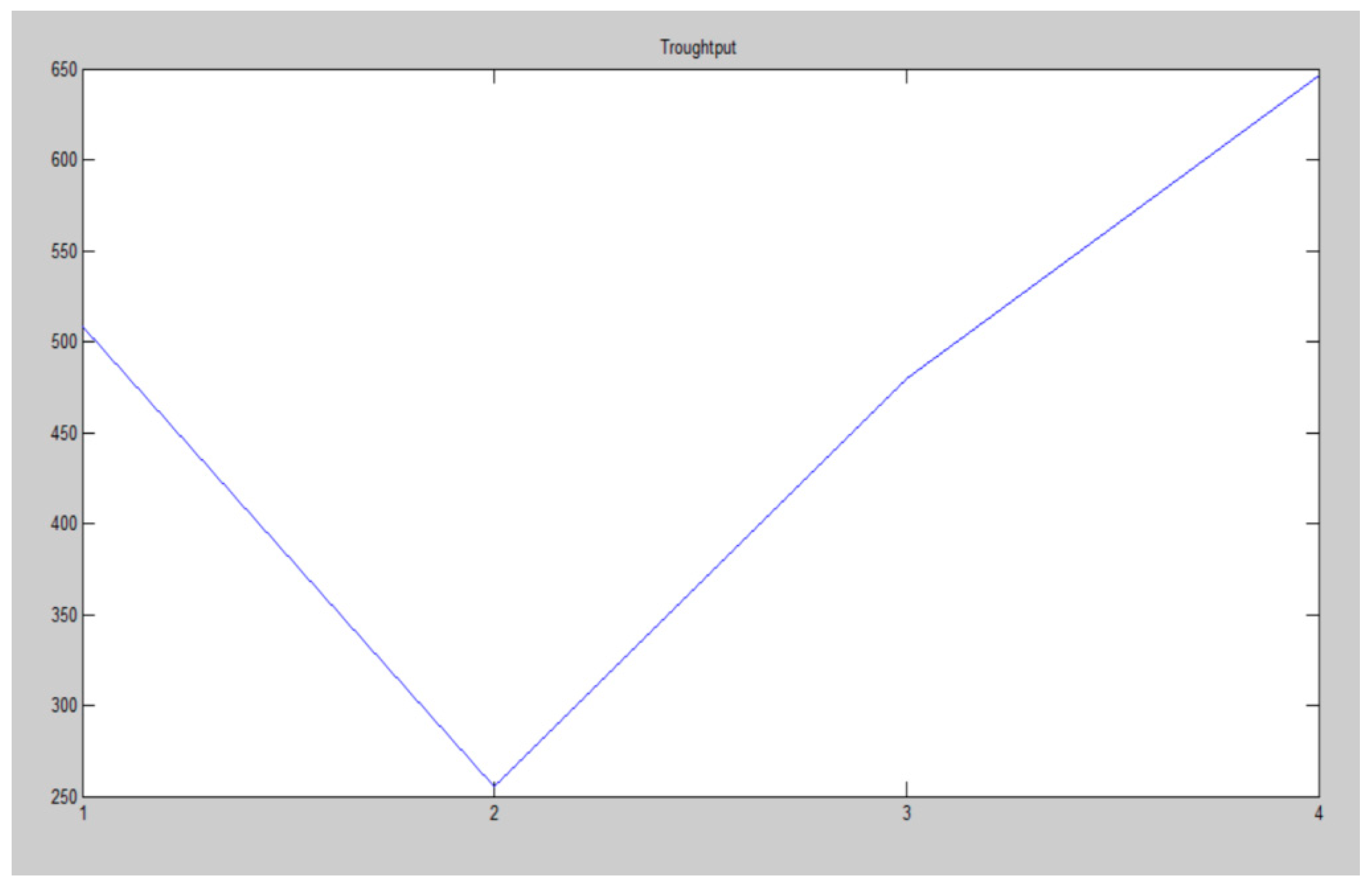
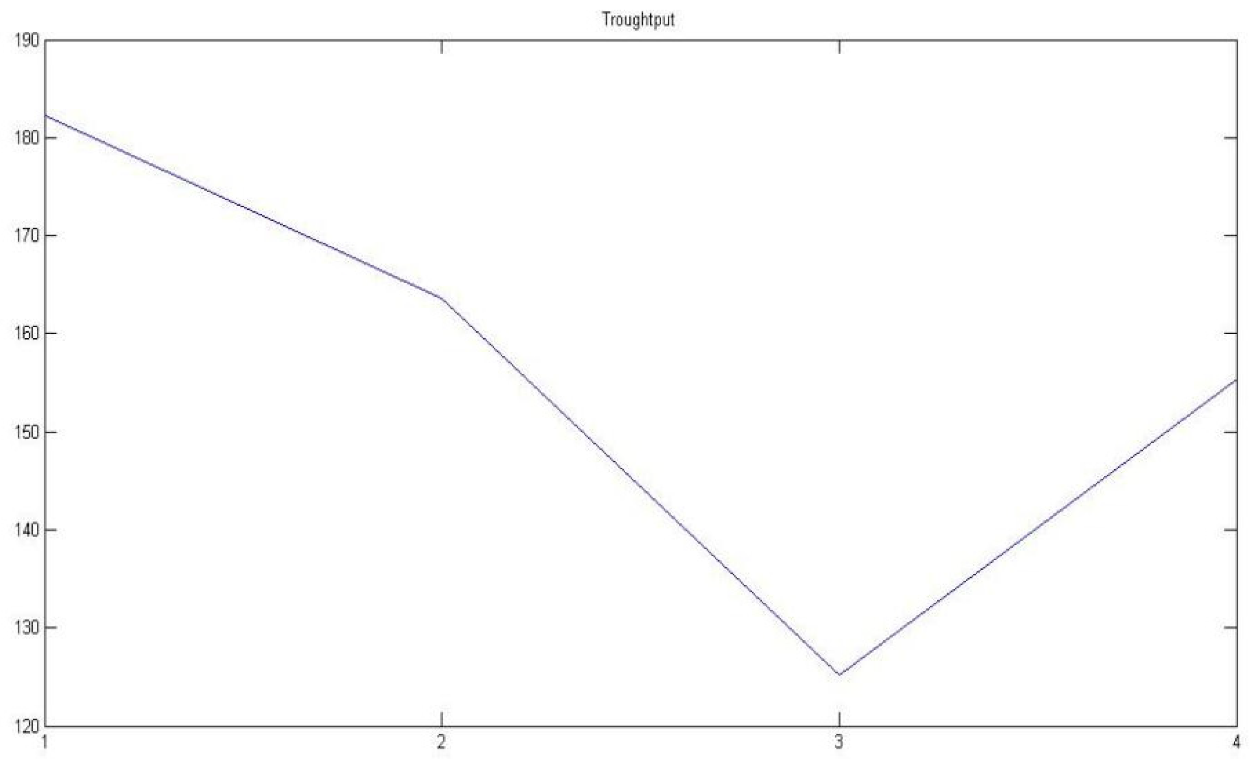
- Throughput
- 2.
- Packet Loss
- 3.
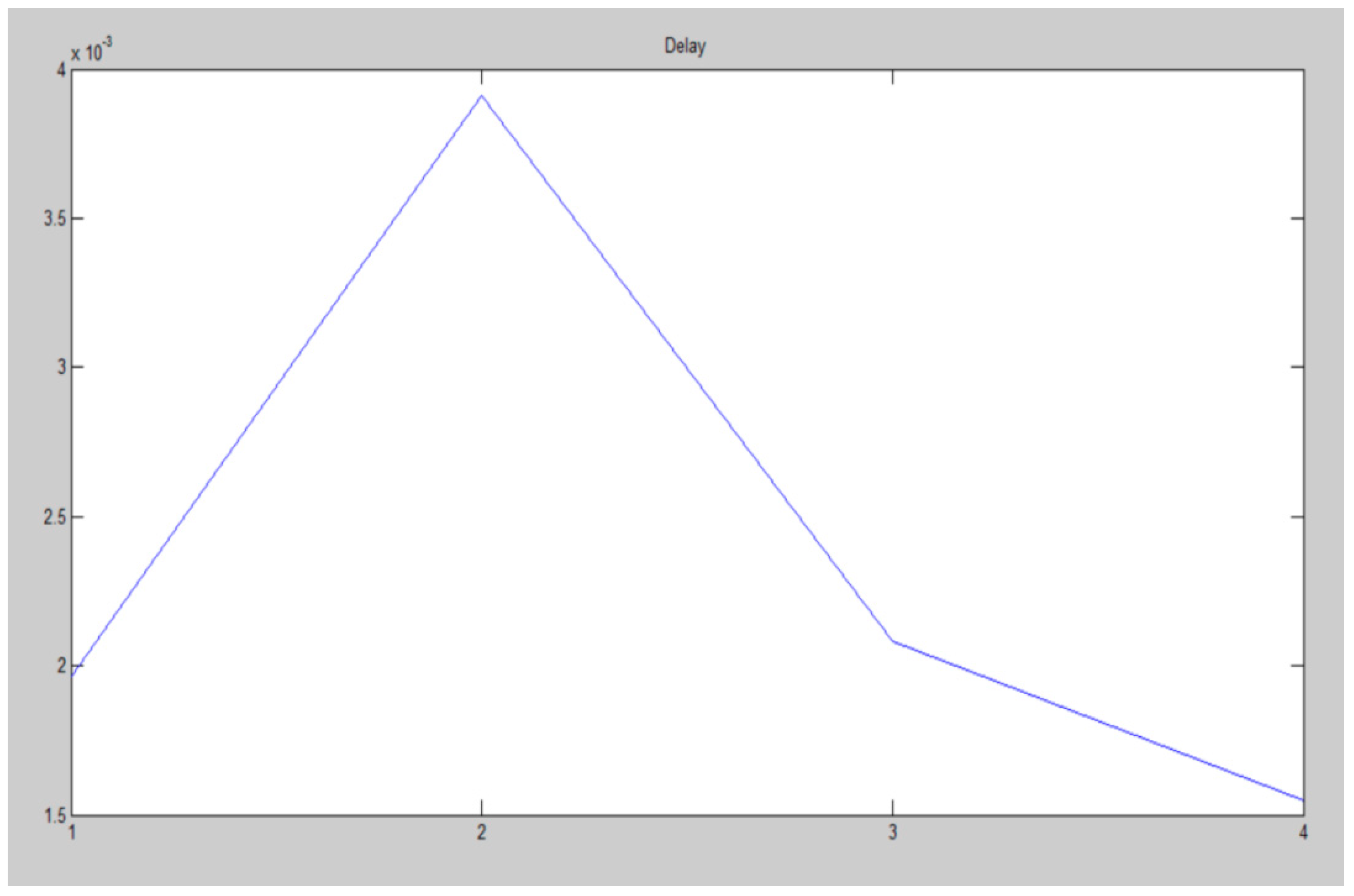
- Delay
4. Discussion
5. Conclusions
Author Contributions
Funding
Institutional Review Board Statement
Informed Consent Statement
Data Availability Statement
Conflicts of Interest
References
- Santhameena, S.; Manikandan, J. Group acknowledgement mechanism for beacon-enabled wireless sensor networks. Comput. Commun. 2022, 187, 93–102. [Google Scholar] [CrossRef]
- Havashemi Rezaeipour, K.; Barati, H. A hierarchical key management method for wireless sensor networks. Microprocess. Microsyst. 2022, 90, 104489. [Google Scholar] [CrossRef]
- Xiong, C.W.; Tang, M.; Wang, X.H.; Liu, Y.; Shi, J. Evolution model of high quality of service for spatial heterogeneous wireless sensor networks. Phys. A: Stat. Mech. Its Appl. 2022, 596, 127182. [Google Scholar] [CrossRef]
- Frey, H.; Stojmenović, I. Geographic and Energy-Aware Routing in Sensor Networks; John Wiley & Sons, Inc.: Hoboken, NJ, USA, 2005. [Google Scholar]
- Rehan, W.; Fischer, S.; Rehan, M.; Rehmani, M.H. A comprehensive survey on multichannel routing in wireless sensor networks. J. Netw. Comput. Appl. 2017, 95, 1–25. [Google Scholar] [CrossRef]
- Hamid, M.A.; Abdullah-Al-Wadud, M.; Chong, I. Multi-channel MAC protocol for wireless sensor networks: A schedule-based approach. In Proceedings of the International Conference on Information Networking, ICOIN 2011, Kuala Lumpur, Malaysia, 26–28 January 2011; pp. 68–73. [Google Scholar] [CrossRef]
- Singhal, C.; Patil, V. HCR-WSN: Hybrid MIMO cognitive radio system for wireless sensor network. Comput. Commun. 2021, 169, 11–25. [Google Scholar] [CrossRef]
- Lavanya, G.; Rani, C.; Ganeshkumar, P. An automated low cost IoT based Fertilizer Intimation System for smart agriculture. Sustain. Comput. Inform. Syst. 2019, 28, 100300. [Google Scholar] [CrossRef]
- Mahesh, N.; Vijayachitra, S. Hierarchical autoregressive bidirectional least-mean-square algorithm for data aggregation in WSN based IoT network. Adv. Eng. Softw. 2022, 173, 103275. [Google Scholar] [CrossRef]
- Cinar, H.; Cibuk, M.; Erturk, I. HMCA WSN: A hybrid multi-channel allocation method for erratic delay constraint WSN applications. Comput. Stand. Interfaces 2019, 65, 92–102. [Google Scholar] [CrossRef]
- Yigit, M.; Gungor, V.C.; Fadel, E.; Nassef, L.; Akkari, N.; Akyildiz, I.F. Channel-aware routing and priority-aware multi-channel scheduling for WSN-based smart grid applications. J. Netw. Comput. Appl. 2016, 71, 50–58. [Google Scholar] [CrossRef]
- Chouikhi, S.; Korbi, I.E.; Ghamri-Doudane, Y.; Azouz Saidane, L. Centralized connectivity restoration in multichannel wireless sensor networks. J. Netw. Comput. Appl. 2017, 83, 111–123. [Google Scholar] [CrossRef]
- Rehan, W.; Fischer, S.; Rehan, M. Anatomizing the robustness of multichannel MAC protocols for WSNs: An evaluation under MAC oriented design issues impacting QoS. J. Netw. Comput. Appl. 2018, 121, 89–118. [Google Scholar] [CrossRef]
- Krishnan, R.S.; Julie, E.G.; Robinson, Y.H.; Raja, S.; Kumar, R.; Thong, P.H.; Son, L.H. Fuzzy Logic based Smart Irrigation System using Internet of Things. J. Clean. Prod. 2020, 252, 119902. [Google Scholar] [CrossRef]
- Yiǧit, M.; Incel, Ö.D.; Güngör, V.Ç. On the interdependency between multi-channel scheduling and tree-based routing for WSNs in smart grid environments. Comput. Netw. 2014, 65, 1–20. [Google Scholar] [CrossRef]
- Rajpoot, V.; Garg, L.; Alam, M.Z.; Sangeeta; Parashar, V.; Tapashetti, P.; Arjariya, T. Analysis of machine learning based LEACH robust routing in the Edge Computing systems. Comput. Electr. Eng. 2021, 96, 107574. [Google Scholar] [CrossRef]
- Chouikhi, S.; El Korbi, I.; Ghamri-Doudane, Y.; Azouz Saidane, L. Distributed connectivity restoration in multichannel wireless sensor networks. Comput. Netw. 2017, 127, 282–295. [Google Scholar] [CrossRef]
- Moorthi; Thiagarajan, R. Energy consumption and network connectivity based on Novel-LEACH-POS protocol networks. Comput. Commun. 2020, 149, 90–98. [Google Scholar] [CrossRef]
- Chen, J.I.-Z.; Hengjinda, P. Enhanced Dragonfly Algorithm based K-Medoid Clustering Model for VANET. J. ISMAC 2021, 3, 50–59. [Google Scholar] [CrossRef]
- Mahapatra, R.P.; Yadav, R.K. Descendant of LEACH Based Routing Protocols in Wireless Sensor Networks. Procedia Comput. Sci. 2015, 57, 1005–1014. [Google Scholar] [CrossRef] [Green Version]
- Achroufene, A.; Chelik, M.; Bouadem, N. Modified CSMA/CA protocol for real-time data fusion applications based on clustered WSN. Comput. Netw. 2021, 196, 108243. [Google Scholar] [CrossRef]
- Rehan, W.; Fischer, S.; Chughtai, O.; Rehan, M.; Hail, M.; Saleem, S. A novel dynamic confidence interval based secure channel prediction approach for stream-based multichannel wireless sensor networks. Ad Hoc Netw. 2020, 108, 102212. [Google Scholar] [CrossRef]
- Arora, V.K.; Sharma, V.; Sachdeva, M. A survey on LEACH and other’s routing protocols in wireless sensor network. Optik 2016, 127, 6590–6600. [Google Scholar] [CrossRef]
- Jacob, I.J.; Darney, P.E. Artificial Bee Colony Optimization Algorithm for Enhancing Routing in Wireless Networks. J. Artif. Intell. Capsul. Netw. 2021, 3, 62–71. [Google Scholar] [CrossRef]
- Sabale, K.; Mini, S. Path planning mechanism for mobile anchor-assisted localization in wireless sensor networks. J. Parallel Distrib. Comput. 2022, 165, 52–65. [Google Scholar] [CrossRef]
- Eswaran, S. Opportunities and Trends of Wireless Communications. IRO J. Sustain. Wirel. Syst. 2022, 4, 102–109. [Google Scholar] [CrossRef]
- Soua, R.; Minet, P. Multichannel assignment protocols in wireless sensor networks: A comprehensive survey. Pervasive Mob. Comput. 2015, 16, 2–21. [Google Scholar] [CrossRef]
- Ribeiro, N.D.S.; Vieira, M.A.M.; Vieira, L.F.M.; Gnawali, O. SplitPath: High throughput using multipath routing in dual-radio Wireless Sensor Networks. Comput. Netw. 2022, 207, 108832. [Google Scholar] [CrossRef]
- Rethfeldt, M.; Brockmann, T.; Beichler, B.; Haubelt, C.; Timmermann, D. Adaptive multi-channel clustering in ieee 802.11s wireless mesh networks. Sensors 2021, 21, 7215. [Google Scholar] [CrossRef]
- Kwong, K.H.; Wu, T.T.; Mchie, C.; Andonovic, I. A Self-organizing Multi-channel Medium Access Control (SMMAC) protocol for wireless sensor networks. In Proceedings of the Second International Conference on Communications and Networking in China, Shanghai, China, 22–24 August 2007; pp. 845–849. [Google Scholar] [CrossRef]
- Le, L.; Rhee, I. Implementation and experimental evaluation of multi-channel MAC protocols for 802.11 networks. Ad Hoc Netw. 2010, 8, 626–639. [Google Scholar] [CrossRef]
- Zhang, J.; Sun, J. A game theoretic approach to multi-channel transmission scheduling for multiple linear systems under DoS attacks. Syst. Control Lett. 2019, 133, 104546. [Google Scholar] [CrossRef]
- Yue, H.; Jiang, Q.; Yin, C.; Wilson, J. Research on data aggregation and transmission planning with Internet of Things technology in WSN multi-channel aware network. J. Supercomput. 2020, 76, 3298–3307. [Google Scholar] [CrossRef]
- Han, S.; Zhang, B.; Chai, S. A novel auxiliary hole localization algorithm based on multidimensional scaling for wireless sensor networks in complex terrain with holes. Ad Hoc Netw. 2021, 122, 102644. [Google Scholar] [CrossRef]
- Harb, H.M.H.; Desuky, A.A.S. Adaboost Ensemble with Genetic Algorithm Post Optimization for Intrusion Detection. Update 2011, 2, 1. Available online: https://www.researchgate.net/publication/266355206_Adaboost_Ensemble_with_Genetic_Algorithm_Post_Optimization_for_Intrusion_Detection (accessed on 29 September 2022).
- Singh, O.; Rishiwal, V.; Chaudhry, R.; Yadav, M. Multi-Objective Optimization in WSN: Opportunities and Challenges. Wirel. Pers. Commun. 2021, 121, 127–152. [Google Scholar] [CrossRef]
- Alkalbani, A.S.; Mantoro, T.; Md Tap, A.O. Improved modified reputation-base trust for wireless sensor networks security. Indian J. Sci. Technol. 2016, 9, 37. [Google Scholar] [CrossRef] [Green Version]
- Sumiharto, R.; Ilma, R.; Rif’Atunnisa, R. Metode Routing Protokol LEACH pada Jaringan Sensor Nirkabel Studi Kasus Sistem Pemantauan Suhu dan Kelembaban Udara. IJEIS Indones. J. Electron. Instrum. Syst. 2019, 9, 87. [Google Scholar] [CrossRef]
- Zuo, C.; Zhao, X.; Wang, H.; Ma, X.; Zheng, S.; Xu, F.; Zhang, Q. A theoretical study of hydrogen-bonded molecular clusters of sulfuric acid and organic acids with amides. J. Environ. Sci. 2021, 100, 328–339. [Google Scholar] [CrossRef]
- Daanoune, I.; Abdennaceur, B.; Ballouk, A. A comprehensive survey on LEACH-based clustering routing protocols in Wireless Sensor Networks. Ad Hoc Netw. 2021, 114, 102409. [Google Scholar] [CrossRef]
- Montesano, F.F.; van Iersel, M.W.; Boari, F.; Cantore, V.; D’Amato, G.; Parente, A. Sensor-based irrigation management of soilless basil using a new smart irrigation system: Effects of set-point on plant physiological responses and crop performance. Agric. Water Manag. 2018, 203, 20–29. [Google Scholar] [CrossRef]
- Sharma, D.; Tomar, G.S. Comparative energy evaluation of lEACH protocol for monitoring soil parameter in wireless sensors network. Mater. Today Proc. 2018, 29, 381–386. [Google Scholar] [CrossRef]
- Zhang, J.; Mao, H. Multi-factor identity authentication protocol and indoor physical exercise identity recognition in wireless sensor network. Environ. Technol. Innov. 2021, 23, 101671. [Google Scholar] [CrossRef]
- Sulistyo, F.; Mustika, F. Load balancing protocol leach in wireless sensor network. In Proceedings of the Conference of Electrical Engineering, Telematics, Industrial Technology, and Creative Media, Yogyakarta, Indonesia, 30 November 2019; pp. 25–31. [Google Scholar]
- Farooqi, M.Z.; Tabassum, S.M.; Rehmani, M.H.; Saleem, Y. A survey on network coding: From traditional wireless networks to emerging cognitive radio networks. J. Netw. Comput. Appl. 2014, 46, 166–181. [Google Scholar] [CrossRef]
- Mkongwa, K.G.; Liu, Q.; Wang, S. An adaptive backoff and dynamic clear channel assessment mechanisms in IEEE 802.15.4 MAC for wireless body area networks. Ad Hoc Netw. 2021, 120, 102554. [Google Scholar] [CrossRef]
- Derdar, A.; Bensiali, N.; Adjabi, M.; Boutasseta, N.; Bouakkaz, M.S.; Attoui, I.; Fergani, N.; Bouraiou, A. Photovoltaic energy generation systems monitoring and performance optimization using wireless sensors network and metaheuristics. Sustain. Comput. Inform. Syst. 2022, 35, 100684. [Google Scholar] [CrossRef]
- Hidalgo-Leon, R.; Urquizo, J.; Silva, C.E.; Silva-Leon, J.; Wu, J.; Singh, P.; Soriano, G. Powering nodes of wireless sensor networks with energy harvesters for intelligent buildings: A review. Energy Rep. 2022, 8, 3809–3826. [Google Scholar] [CrossRef]
- Al-Sodairi, S.; Ouni, R. Reliable and energy-efficient multi-hop LEACH-based clustering protocol for wireless sensor networks. Sustain. Comput. Inform. Syst. 2018, 20, 1–13. [Google Scholar] [CrossRef]
- Bristow, K.L.; Šimůnek, J.; Helalia, S.A.; Siyal, A.A. Numerical simulations of the effects furrow surface conditions and fertilizer locations have on plant nitrogen and water use in furrow irrigated systems. Agric. Water Manag. 2020, 232, 106044. [Google Scholar] [CrossRef]
 = Cluster head,
  = Cluster member.


| Parameter | Value |
|---|---|
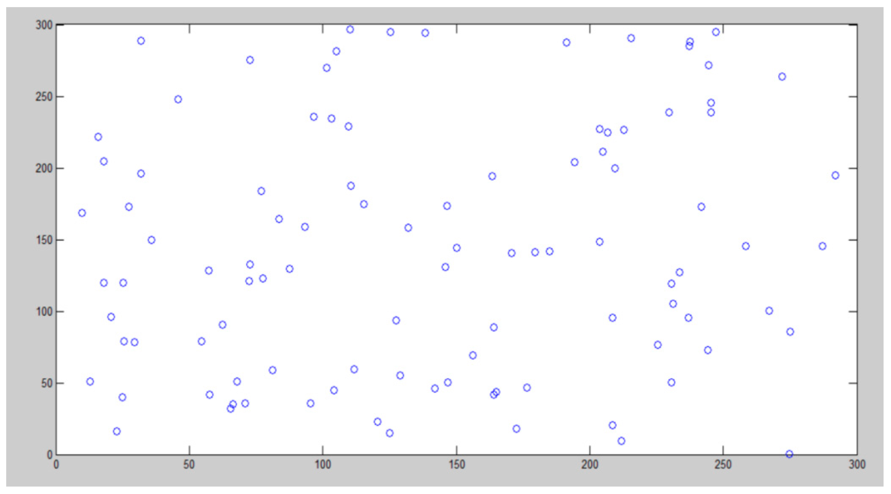
| Number of nodes | 100 |
| Energy | 100 |
| Xmax | 300 |
| Ymax | 300 |
| Velocity | 10,000 |
| Algorithm 1: Temperature and Humidity Criteria Algorithm |
| n = 100; N = 4; energy = 100; temp_top = 26; temp_bot = 20; humi_top = 100; humi_bot = 0; huma_top = 100; huma_bot = 0; freq_top = 50; freq_bot = 10; xmax = 300; ymax = 300; velocity = 10,000; for i = 1:n node(i).id = i; node(i).xd = (xmax).* rand(1,1); node(i).yd = (ymax).* rand(1,1); node(i).energy = energy; node(i).temp = (temp_top − temp_bot).* rand(1,1) + temp_bot; node(i).humi = (humi_top − humi_bot).* rand(1,1) + humi_bot; node(i).huma = (huma_top − huma_bot).* rand(1,1) + huma_bot; node(i).freq = (freq_top − freq_bot).*rand(1,1) + freq_bot; axis([0 xmax 0 ymax]) plot(node(i).xd,node(i).yd,’o’); hold on end clear energy temp_top temp_bot humi_top humi_bot huma_top huma_bot freq_top freq_bot |
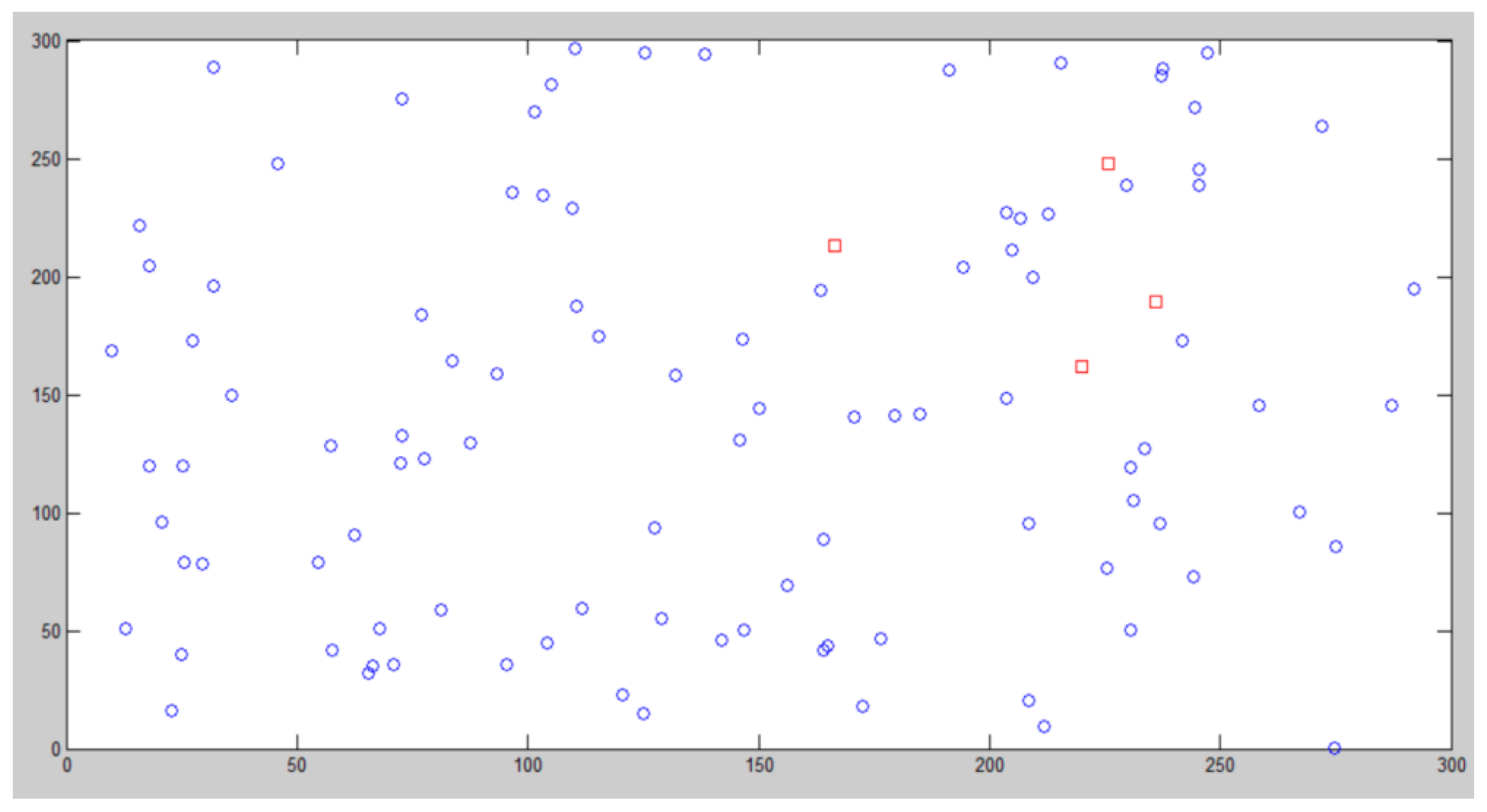
| Algorithm 2: cluster head selection |
| cent = struct(); hold on for k = 1:N cent(k).x = (b − a).* rand(1,1) + a; cent(k).y = (b − a).* rand(1,1) + a; plot(cent(k).x,cent(k).y,’s red’); hold on end figure(2) for k = 1:N plot(cent(k).x,cent(k).y,’s red’); hold on end dis = struct(); for i = 1:n plot(node(i).xd,node(i).yd,’o’); hold on for k = 1:N dis(i).cent(k).id = k; dis(i).cent(k).distance = pdist ([node(i).xd, node(i).yd; cent(k).x, cent(k).y],’euclidean’); end end clustering_channel = struct(); count = 0; for k = 1:N for i = 1:n if node(i).cent == k count = count + 1; clustering_channel(k).node(count) = node(i).id; end end count = 0; end |
| Algorithm 3: Calculation of the distance between each node and cluster head |
| for k = 1:N for i = 1:size(clustering_channel(k).node,2) p = clustering_channel(k).node(i); hac(k).ch(i).id = node(p).id; for j = 1:size(clustering_channel(k).node,2) hac(k).ch(i).d(j).id = clustering_channel(k).node(j); end end [~,index] = sortrows ([hac(k).ch(i).d.dis].’); hac(k).ch(i).d = hac(k).ch(i).d(index); clear index end iter = 0; x = zeros(); for i = 1: size(node,2) if node(i).cent end end y = pdist(x); Y = squareform(y); z = linkage(y); figure() dendrogram(z) title(strcat(‘Channel-’, num2str(k))) D = 0; for i = 1:size(z,1) D = D + z(i,3); end HAC(k).distance = D; sc = size(clustering_channel(k).node,2); F = 0; for i = 1:size(z,1) n1 = z(i,1); n2 = z(i,2); if n1 <= sc && n2 <= sc F = F + 1; end end I = inconsistent(z); loss = 0; for i = 1:size(I,1) loss = loss + I(i,4); end end |
| Algorithm 4: The process of forming a WSN channel |
| for k = 1:N for i = 1:size(clustering_channel(k).node,2) end end xx = 1:1:N; for i = 1:N−1 end for i = 1:N−1 end title(‘Delay’) for i = 1:N−1 plot ([xx(i) xx(i + 1)], [HAC(i).throughtput HAC(i + 1).throughtput]) hold on end for i = 1:N−1 end |
| Channel 1 | Node |
|---|---|
| 6, 7, 11, 12, 13, 14, 15, 17, 24, 25, 26, 29, 31, 33, 37, 38, 40, 43, 47, 50, 57, 67, 68, 71, 74, 76, 78, 82, 83, 85, 87, 89, 90, 91, 94, 95, 97, 98, 99, 100 |
| Channel 2 | Node |
|---|---|
| 3, 49, 53, 60, 93 |
| Channel 3 | Node |
|---|---|
| 2, 10, 16, 18, 20, 21, 22, 23, 27, 28, 30, 32, 35, 36, 39, 41, 42, 44, 45, 46, 48, 51, 54, 55, 56, 58, 59, 61, 62, 63, 64, 69, 72, 75, 77, 79, 80, 81, 84, 86, 88, 92 |
| Channel 4 | Node |
|---|---|
| 1, 4, 5, 8, 9, 19, 34, 52, 65, 66, 70, 73, 96 |
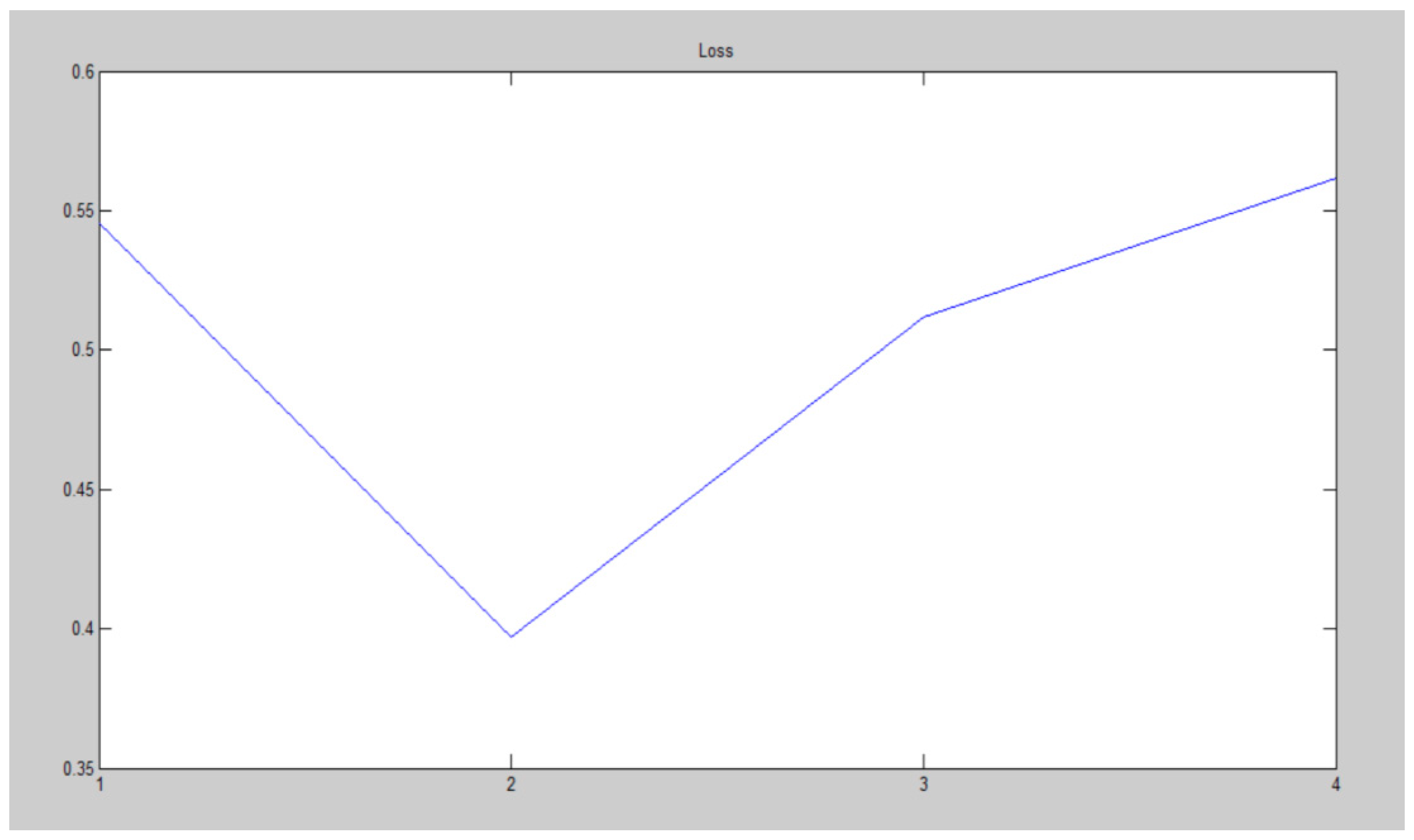
| Channels | Parameters |
|---|---|
| Channel 1 | 0.5455 |
| Channel 2 | 0.3968 |
| Channel 3 | 0.5120 |
| Channel 4 | 0.5616 |
| Channels | Parameters |
|---|---|
| Channel 1 | 0.0020 |
| Channel 2 | 0.0039 |
| Channel 3 | 0.0021 |
| Channel 4 | 0.0015 |
| Channels | Parameters |
|---|---|
| Channel 1 | 766.9368 |
| Channel 2 | 156.5153 |
| Channel 3 | 854.4712 |
| Channel 4 | 185.5971 |
| Channels | Parameters |
|---|---|
| Channel 1 | 508.5165 |
| Channel 2 | 255.5661 |
| Channel 3 | 479.8289 |
| Channel 4 | 646.5618 |
| Channels | Parameters |
|---|---|
| Channel 1 | 190 |
| Channel 2 | 165 |
| Channel 3 | 125 |
| Channel 4 | 158 |
Publisher’s Note: MDPI stays neutral with regard to jurisdictional claims in published maps and institutional affiliations. |
© 2022 by the authors. Licensee MDPI, Basel, Switzerland. This article is an open access article distributed under the terms and conditions of the Creative Commons Attribution (CC BY) license (https://creativecommons.org/licenses/by/4.0/).
Share and Cite
Rizky, R.; Mustafid; Mantoro, T. Improved Performance on Wireless Sensors Network Using Multi-Channel Clustering Hierarchy. J. Sens. Actuator Netw. 2022, 11, 73. https://doi.org/10.3390/jsan11040073
Rizky R, Mustafid, Mantoro T. Improved Performance on Wireless Sensors Network Using Multi-Channel Clustering Hierarchy. Journal of Sensor and Actuator Networks. 2022; 11(4):73. https://doi.org/10.3390/jsan11040073
Chicago/Turabian StyleRizky, Robby, Mustafid, and Teddy Mantoro. 2022. "Improved Performance on Wireless Sensors Network Using Multi-Channel Clustering Hierarchy" Journal of Sensor and Actuator Networks 11, no. 4: 73. https://doi.org/10.3390/jsan11040073