Design, Analysis, and Simulation of 60 GHz Millimeter Wave MIMO Microstrip Antennas

Abstract

This article comparatively shows the evolution of parameters of three types of arrays for MIMO microstrip antennas, to which the number of ports is gradually incremented until reaching 32. The three arrays have a 1 × 2 configuration in each port and present different geometry or type of coupling in the next way: square patch with quarter-wave coupling (Antenna I), square patch with inset feed (Antenna II) and circular patch with quarter-wave coupling (Antenna III). The arrays were designed and simulated to operate on the millimetric wave band, specifically in the 60 GHz frequency to be used in wireless technologies such as IEEE 802.11 ad. A method of rapid prototyping was formulated to increase the number of elements in the array obtaining dimensions and coordinates of location in the layout in short periods of time. The simulation was conducted through ADS software, and the results of gain, directivity, return loss, bandwidth, beamwidth, and efficiency were evaluated. In terms of array results of 32 ports, Antenna III obtained the lowest return loss with −42.988 dB, being more than 19 dB lower than the others. The highest gain is also obtained by Antenna III with 24.541 dBi and an efficiency of 66%. Antenna II obtained better efficiency, reaching 71.03%, but with a gain of more than 2dB below the Antenna III. Antenna I obtained the best bandwidth.

1. Introduction

The radio spectrum is a resource with which more applications live nowadays, many of them with high bandwidth consumption due to the evolution of digital technologies and the high demand of wireless connections from people and systems. The use of the lowest range of this spectrum has been widely utilized because of the simplicity of propagation that allows for advantages of coverage and minimizes the installed infrastructure. With the advantages of propagation presented in these frequencies, the spectrum has been saturated in this range, preventing modern technologies from accessing higher bandwidths; however, in higher frequency bands, there is enough available bandwidth, but with bigger problems in the propagation of the signal. The availability of higher bandwidths opens the possibility of operating in frequency ranges from 24 to 100 GHz; these signals are within the band of millimetric waves (mmWave). For the use of millimetric wave bands, the deployment of a bigger amount of infrastructure is planned to provide less coverage so that the signal propagation distances are not too long. Incidentally, the development of technologies such as massive MIMO and beamforming would be of great help for the optimization of energy use and the reduction in mobile communication interference using millimetric waves. In this sense, it is pertinent to evaluate different types of arrays of MIMO antennas with the purpose of obtaining more efficient designs and optimizing the energy transmitted in mobile technologies such as Wi-Fi, Bluetooth, IoT, 5G, among others [1].

Considering the importance of the array in MIMO antennas in the implementation of wireless technologies in millimetric wave bands, designing and evaluating different configurations are sought for, which are capable of transmitting or receiving a determined range of frequencies. The computational development in recent years has allowed for the implementation of electromagnetic simulation software, which enables the modeling of phenomena related to the radiation of antennas, in a way that their behavior can be predicted with high precision before actual implementation and testing. Some of the antennas that can be modeled with great precision by means of this type of software are microstrip antennas; these antennas appeared in 1950 [2] and are currently widely used in different wireless devices, given that their implementation is done on PCB (printed circuit board). This work shows the design and simulation of arrays of MIMO microstrip antennas working in the 60 GHz frequency, one of the work frequencies of Wi-Fi IEEE 802.11 ad [3]. Working with microstrip technology provides advantages such as the easy incorporation in latest-technology devices and the great availability of tools for the design and simulation process. On the other hand, some unfavorable points for these antennas should be considered, such as their relatively narrow bandwidth, management of low frequency in any worked frequency, and low efficiency. One of the reasons to use such technology in array of MIMO antennas is that it enables an efficient management of power, and in comparison to other types of antennas, the biggest advantage of the microstrip technology is its low fabrication cost and the lack of necessity of a powerful feeding source for its proper functioning [1,4,5,6].

In the last few years, different studies have geared towards the development of antennas that work in the millimetric wave frequency band. Initially, developments are shown with microstrip antennas simulated or made with FR-4 substrate. In [7], the design of an antenna is proposed for a frequency of 1930.8 MHz. It is proved that the exact measurements of the utilized substrate must be at hand in order to obtain good results in practice. When implementing the antenna in a real environment, a return loss of −27 dB was measured in an operation frequency of 1929.6 MHz, which represents an error of 1 MHz in relation to the desired frequency. It is concluded that with more exact substrate data, results in simulation and in a real environment improve until reaching the frequency of 1930.8 MHz. In [8,9], the antenna development to work in the WiMAX technology operating in the 3.5 and 5.5 GHz band is found. The set goal is to reduce mutual coupling caused by MIMO technology given that it places multiple antennas in the same patch. Regarding this, two possible solutions are established, the first one uses resounding elements that minimize the mutual coupling effect, and the second one starts from having a minimum spacing of 0.5 λ (Wavelength) between antennas. In [10], the development of 2 × 2 MIMO antennas is shown working in a frequency of 28 and 38 GHz, highlighting parameters of the designed antennas such as the result of return loss reaching values of −54 and −51 dB and a high efficiency of 98%. This design is set for 5 g technologies. In [11], a small antenna design is elaborated reaching a 10 × 12 mm² size working a unique frequency of 28 GHz with the purpose of being used in 5 g communication devices and IoT technology. In [12], a simulation is presented to a frequency of 60 GHz with an array of 1 × 2 base antenna in each port, with the aim of reaching high gain. The development of different tests is shown increasing the number of ports to 16. A gain of 19.89 dBi was reached, a directivity of 21.59 dBi and an efficiency of 67.57%. This antenna is destined to work in 5G and 802.11 ad. The developments of microstrip antennas involve the measurement of different parameters to establish its performance. These parameters can be bandwidth, gain, directivity, return loss, efficiency, among others [13,14,15,16,17,18,19,20]. In the review of the state of the art related to microstrip antennas that work at high frequencies, comparative studies were not found to establish the performances of MIMO antenna arrays with different geometries or types of coupling that work in the same frequency. There is no evidence either of methodologies of rapid prototyping that allow for designing, simulating, increasing the number of elements, or rapidly finding operating parameters to validate the performance of the antenna. This article presents the design, simulation, and performance evaluation of three types of MIMO antennas array of maximum 32 ports each. Each port is connected to a 1 × 2 array of one of the three types of antennas: square patch with quarter-wave coupling (Antenna I), square patch with inset feed (Antenna II), and circular patch with quarter-wave coupling (Antenna III). As part of the development, a method of rapid prototyping is established for the design and simulation of microstrip antenna arrays. This methodology will be a useful tool for the design, simulation, and performance evaluation of other microstrip antenna arrays.

For the development of this research, the ADS (advanced design system) [21] simulation tool was used; ADS uses the method of moment to model the electromagnetic behavior of antennas. This numeric method allows for establishing the different parameters of antennas accurately; it also allows for running simulations of microstrip MIMO antennas with the required number of ports. From the simulation parameters, such as gain, directivity, efficiency, and return loss, 3d and 2d radiation diagrams can be extracted, among others.

The article is organized in five sections. In Section 1, an introduction about the purpose of the research is elaborated. In Section 2, the proposed methodology is presented, which is divided into five phases: Phase A, design parameters; Phase B, design of Antenna I, taking the work done in [12] as the starting point; Phase C, design of Antenna II; Phase D, design of Antenna III; lastly, in Phase E, a method of rapid prototyping and simulation of antennas is proposed; the antennas are drawn from Cartesian coordinates to finally be located in the ADS software. In Section 3, the discussion and the obtained results are presented. In this section, the way the geometry of antennas affects the obtained parameters is established, as well as the impedance coupling in square patch antennas, and which antenna obtained better results to work in the desired frequency. In Section 4, the conclusions of the present work are disclosed, and the references are found at the end.

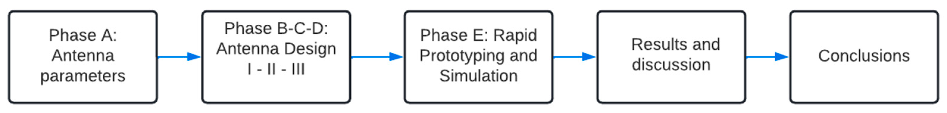
2. Methodology

Figure 1 shows the methodology used in the development of the research. Initially, characteristics of antennas were established such as design frequency and type of material used. Subsequently, design calculations were performed for each of the three microstrip basic antennas: square patch with quarter-wave coupling length (Antenna I), square patch with inset feed (Antenna II), and circular patch with quarter-wave coupling length (Antenna III). In this design stage, calculations of the transmission lines are also performed according to their impedance, and the 1 × 2 array dimensions that connect each port are established. As simulating arrays of different sizes is intended, a rapid prototyping method is established to perform calculations and increase the number of ports for each array, so that the used software tools deliver the dimensions automatically replicating the base array (1 × 2 array) any number of times desired. In this case, antennas of 1, 2, 4, 6, 8, 12, 16, and 32 ports were simulated for each type of antenna. In the final phase, the calculated parameters in the antenna arrays are analyzed.

2.1. Phase A. Parameters of the Antennas

In this phase of the methodology, the antenna parameters of operation are defined. One of the fundamental aspects for the success in the implementation of the antenna, is the knowledge of the substrate parameters, because the calculations and the simulation vary with small changes in this material. In previous works, it was evident that the most used materials are Rogers Duroid 5880 and FR4 [22]. In

Table 1. FR-4 substrate parameters.

Parameter	Value
$f_r=operation frequency$	$60 \mathrm{GHz}$
$T_l=Loss Tangent$	$0.0004$
${\epsilon }_r=Substrate dielectric constant$	$4.4$
${\epsilon }_0=Permittivity Constant$	$8.8542\cdot {10}^{-12}\frac{{\mathrm{C}}^2}{{\mathrm{Nm}}^2}$
$h or d=Substrate thickness$	$0.2 \mathrm{mm}$
$V_0 or C=Speed of Light$	$3\cdot {10}^8 \frac{\mathrm{m}}{\mathrm{s}}$

, the parameters with which the mathematical calculations and the simulation will be made are shown. The chosen substrate is FR-4, which was also used in [12,23] for the development of microstrip antennas.

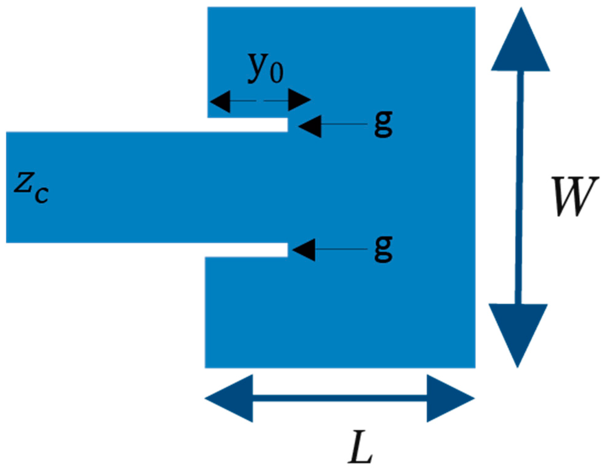
2.2. Phase B. Design of Antenna I

In this phase, the square patch antenna with quarter-wave coupling length is designed. In Figure 2, the geometry of the antenna is shown, as well as the notation utilized for its dimensions. Following this, the equations with which dimensions were determined are shown. Equation (1) allows for finding width W.

$$W=\frac{v_0}{2-f_r}\sqrt{\frac{2}{{\epsilon }_r+1}}$$

(1)

Length L is determined using equations from (2) to (5). In (2), ${\epsilon }_{reff}$is found, which corresponds to the effective permittivity of the dielectric. Subsequently, all variables necessary for the calculation are determined.

$$\frac{W}{h}>1 , {\epsilon }_{reff}=\frac{{\epsilon }_r+1}{2}+\frac{{\epsilon }_r-1}{2}{\left[1+12\frac{h}{w}\right]}^{-\raisebox{1ex}{$1$}\!\left/ \!\raisebox{-1ex}{$2$}\right.}$$

(2)

The value of ∆L is determined solving (3), and the value of $L_{eff}$, which corresponds to patch effective length, using (4) [24].

$$\frac{\Delta L}{h}=0.412\frac{\left({\epsilon }_{reff}+0.3\right)\left(\frac{w}{h}+0.264\right)}{\left({\epsilon }_{reff}-0.258\right)\left(\frac{w}{h}+0.8\right)}$$

(3)

$$L_{eff}=\frac{c}{2f_r\sqrt{{\epsilon }_{reff}}}$$

(4)

The actual length considers the results obtained in (3) and (4), replacing $\Delta L$ and $L_{eff}$ in (5).

$$L=L_{eff}-2\Delta L$$

(5)

Once patch data have been found, impedance is calculated in the feeding point ($R_{in}$). Through (6), the wavelength ${\lambda }_0$ is determined [22], as well as the conductance on the border of the patch through (7) [25].

$${\lambda }_0=\frac{c}{f_r}$$

(6)

$$G_e=0.00836\frac{w}{{\lambda }_0}$$

(7)

Considering the result obtained in Equation (7), impedance is calculated on the border of patch ($R_{in}$) using (8).

$$R_{in}=\frac{1}{\left(2G_e\right)}$$

(8)

Impedance of the transmission line $Z_c$ is 50 Ω; therefore, impedance of the quarter-wave transformer $Z_1$ is calculated, replacing $R_{in}$ and $Z_c$ in Equation (9) [22]:

$$Z_1=\sqrt{Z_c{R}_{in}}$$

(9)

Once the values of the transmission lines impedance have been obtained, their dimensions are calculated using Equations (10) to (15); Figure 3 shows the dimensions of a microstrip transmission line on the selected substrate.

The transmission line width $\left(Wt\right)$ is calculated using Equations (10)–(12), where $Z_0$ corresponds to the impedance of the segment of the transmission line to be calculated [26]; in the case of Figure 2, the calculation must be made independently for $Z_1$ and $Z_c$.

$$A=\frac{z_0}{60}\sqrt{\frac{{\epsilon }_r+1}{2}}+\frac{{\epsilon }_r-1}{{\epsilon }_r+1}\left(0.23+\frac{0.11}{{\epsilon }_r}\right)$$

(10)

$$B=\frac{377\pi }{\left(2Z_0\sqrt{{\epsilon }_r}\right)}$$

(11)

$$\frac{Wt}{d}=\{\begin{array}{ll}\frac{8{\mathrm{e}}^A}{{\mathrm{e}}^{2A}-2}& para Wt/d<2\\ \frac{2}{\pi }\left[B-1-\ln \left(2B-1\right)+\frac{{\epsilon }_r-1}{2{\epsilon }_r}\left\{\ln \left(B-1\right)+0.39-\frac{0.61}{{\epsilon }_r}\right\}\right]& para Wt/d>2\end{array}$$

(12)

Once the transmission line width has been measured, the effective dielectric constant is calculated (${\epsilon }_{reffLt}$), as well as the phase constant in free space ($k_0$), through Equations (13) and (14); these data will be utilized to obtain the length in the transmission line ($Lt$).

$${\epsilon }_{reffLt}=\frac{{\epsilon }_r+1}{2}+\frac{{\epsilon }_r-1}{2}\frac{1}{\sqrt{1+12\frac{d}{Wt}}}$$

(13)

$$k_0=\frac{2\pi f}{c}=\frac{2\pi }{\lambda }$$

(14)

Replacing values provided by Equations (13) and (14), the length of the transmission line is obtained in Equation (15).

$$Lt=\frac{Dfc\left(\pi /180\right)}{\sqrt{{\epsilon }_{reffLt}} k_0}$$

(15)

As per previous calculations, the dimensions obtained for Antenna I are shown in Section 3.

1 × 2 array is shown in Figure 4. It is formed with two of the antennas from Figure 2 (Base antenna). A power combiner is used with impedances of 100, 50 and 100 Ω in segments 1, 2 and 3 as a feeding point of 1 × 2 array. On the ends 1 and 3 of the power combiner, quarter-wave transformers are implemented with impedance of 70 Ω ($Z_{1}low$), which are connected to the feeding transmission lines of 50 Ω from patches ($R_{in}low$). Dimensions of lines with the mentioned impedances can be calculated with Equations (10) to (15). The antenna of Figure 4 is connected to one of the ports and is replicated N times to form the first type of MIMO array (with N = 1, 2, 4, 6, 8, 12, 16, 32).

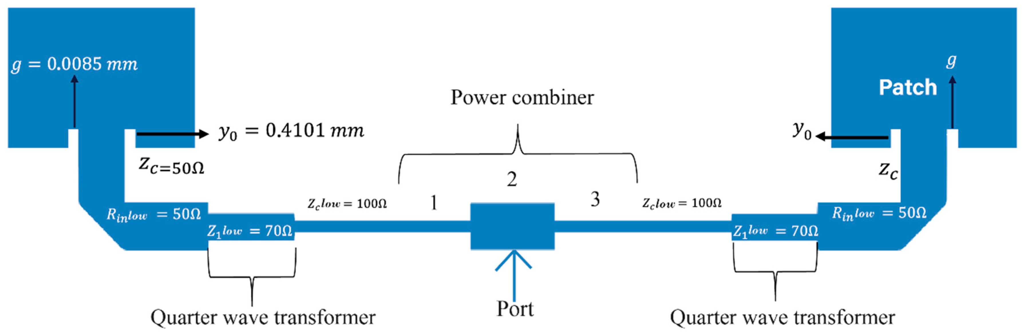
2.3. Phase C. Design of Antenna II

This phase consists of the design of the square patch antenna with inset feed. Figure 5 shows the geometry of the antenna. The objective of the inset feed is to achieve proper impedance coupling by making the transmission line connect to an internal point of the patch. The size of the resulting 1 × 2 array is smaller since a quarter-wave transformer will not be used in the antenna source. To find the patch width and length (W and L), Equations (1) to (5) were used. The estimation of depth $y_0$ involves Equations (16) to (22), and the inset feed width $g$ is calculated by means of Equation (23).

The transmission line (Z_c) in Figure 5 has a 50 Ω impedance, and its dimensions are determined by Equations (10) to (15).

To calculate $y_0$, it is necessary to determine impedance on the border of the patch $R_{in}$ first. Impedance $R_{in}$ is found considering the conductance at the opposite end of the feeding point ($G_1$) and the mutual conductance between the opposite sides of the antenna ($G_{12}$). To begin with, $k_0$ is found by means of (16) [23].

$$k_0=\frac{2\pi f}{c}=\frac{2\pi }{\lambda }$$

(16)

An intermediate step to find $G_1$ is the estimation of $I_1$ by means of Equation (17) [22].

$$I_1={{\displaystyle \int }}_0^{\pi }{\left[\frac{sin\left(\frac{k_{0}w}{2}cos\theta \right)}{cos\theta }\right]}^2{sin}^3\theta \mathrm{d}\theta$$

(17)

When $I_1$ is obtained, $G_1$ is found by using (18).

$$G_1=\frac{I_1}{120{\pi }^2}$$

(18)

Mutual conductance $G_{12}$ is calculated with Equation (19), where $J_0$ is the Bessel function of the first kind of order zero. Impedance $R_{in}$is obtained by using (20).

$$G_{12}=\frac{1}{120{\pi }^2}{{\displaystyle \int }}_0^{\pi }{\left[\frac{\mathit{sin}\left(\frac{k_{0}w}{2}\mathit{cos}\theta \right)}{\mathit{cos}\theta }\right]}^2{J}_0\left(k_{0}L\mathit{sin}\theta \right){\mathit{sin}}^3\theta \mathrm{d}\theta$$

(19)

$$R_{in}=\frac{1}{2\left(G_1\pm G_{12}\right)}$$

(20)

Once the impedance on the border of the patch is obtained, the calculation of the depth of the notch $y_0$ follows. When solving Equation (21), $y_0$ is obtained from (22).

$$z_0=R_{in}{\mathit{cos}}^2\left(\frac{\pi }{L}{y}_0\right)$$

(21)

$$y_0=acos\left(\sqrt{\frac{z_0}{R_{in}}}\right)\ast \frac{L}{\pi }$$

(22)

The inset feed width ($g$) is found with Equation (23) [4].

$$\mathrm{g}=\frac{v_0}{\sqrt{2{\epsilon }_{reff}}}\ast \frac{4.65\ast {10}^{-12}}{f\left(GHz\right)}$$

(23)

Figure 6 shows the final setting of the 1 × 2 array of patch antenna with inset feed. The connection to the power combiner was performed similarly to Antenna I.

During the simulation phase of this antenna, the inset feed depth values were optimized by slightly modifying its dimensions to achieve better results for a 60 GHz frequency. In the Section 3 will be shown the final dimensions of the array.

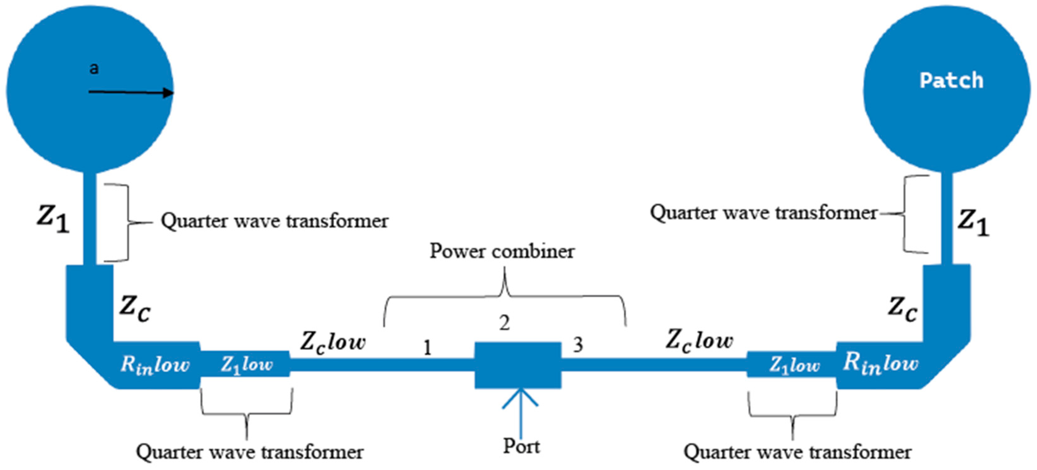
2.4. Phase D. Design of Antenna III

This phase contains the calculations to determine the dimensions of the circular Microstrip Antenna with quarter-wave coupling. The 1 × 2 array is shown in Figure 7, where the radius ($a$) is found by means of Equations (24) and (25). By using (24), $F$ is found, which is a necessary variable to determine the value of $a$ by using (25).

$$F=\frac{8.791\ast {10}^9}{f_r\sqrt{{\epsilon }_r}}$$

(24)

$$a=\frac{F}{{\left\{1+\frac{2h}{\pi {\epsilon }_{r}F}\left[\ln \left(\frac{\pi F}{2h}\right)+1.7726\right]\right\}}^{\raisebox{1ex}{$1$}\!\left/ \!\raisebox{-1ex}{$2$}\right.}}$$

(25)

In Figure 7, the dimensions of transmission lines, quarter-wave transformer, and power combiner are the same as those for Antenna I.

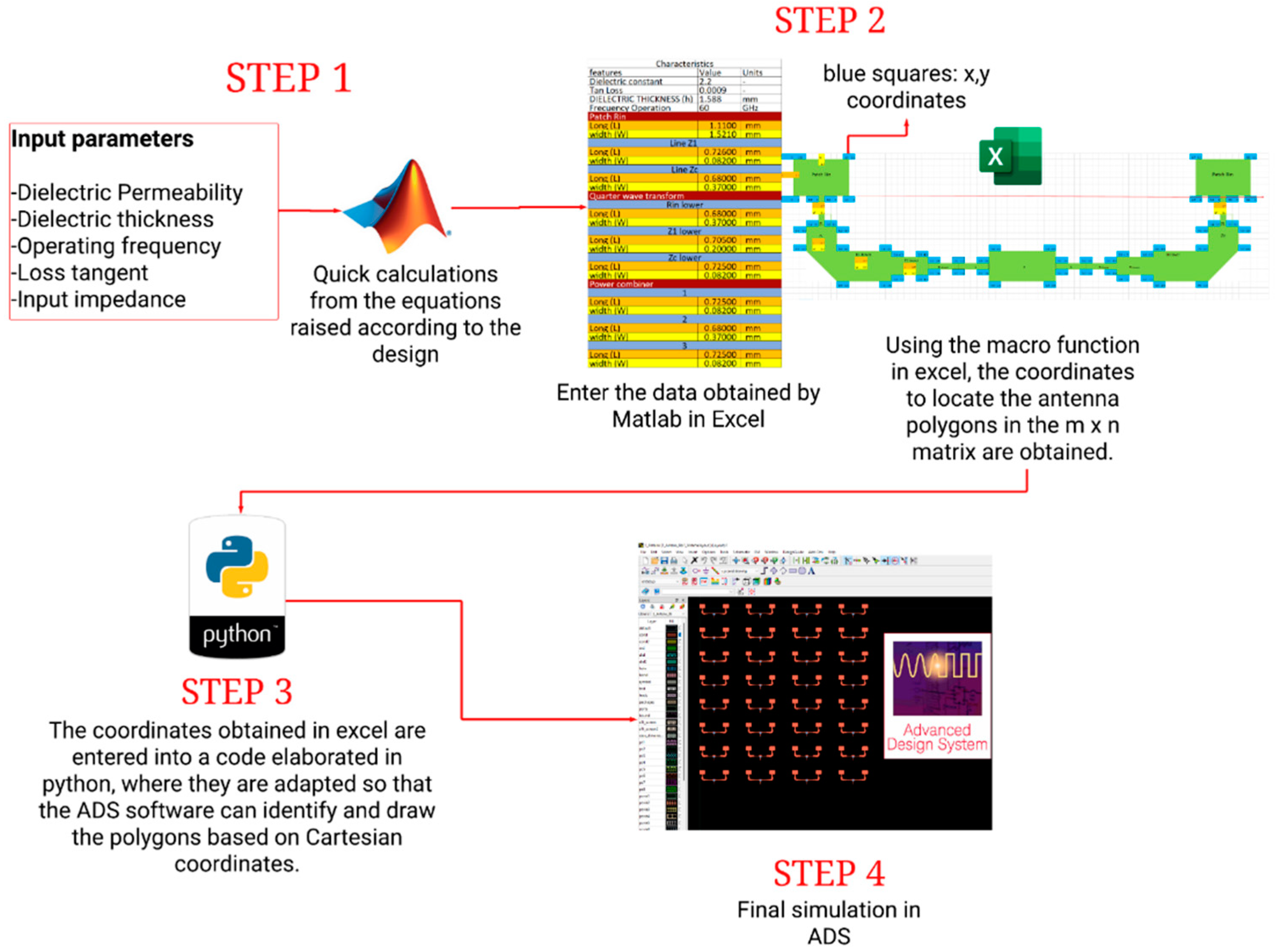
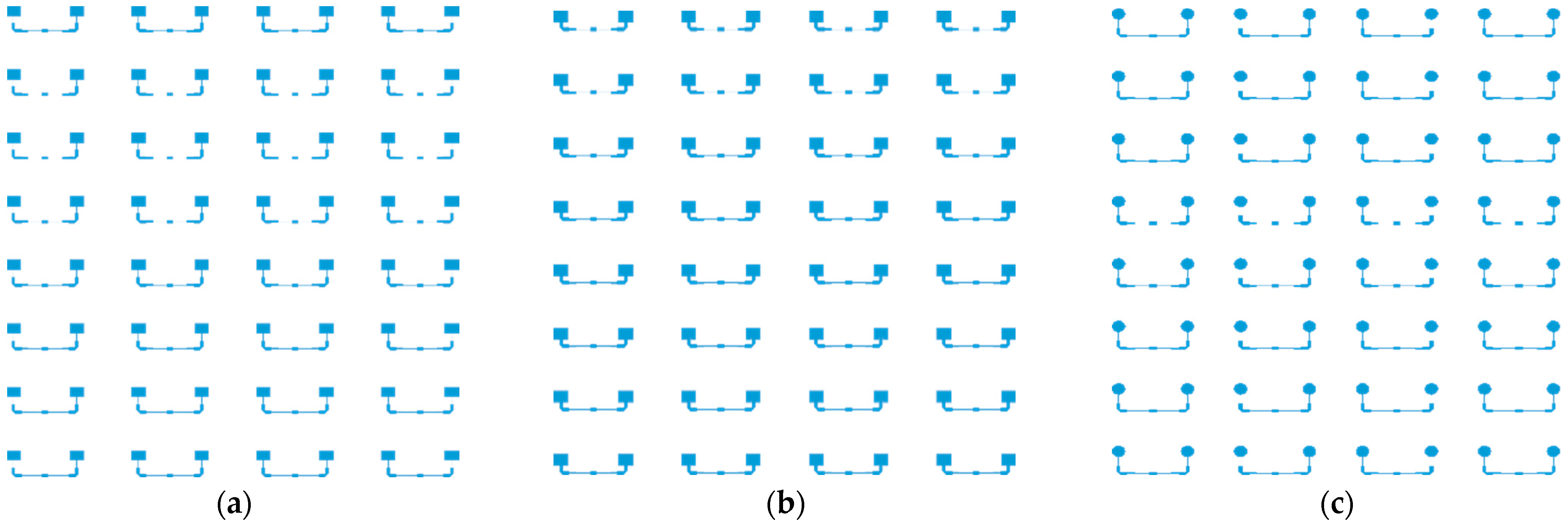
2.5. Phase E. Rapid Prototyping and Simulation

A rapid prototyping method was developed to perform calculations, establish implementation coordinates, and increase the number of elements in an array. The array dimensions can be digitized into the ADS software by means of console commands. The input data of the rapid prototyping process are the characteristics of the antenna design and the substrate, while the output is the sketch of the array on the ADS software template. Different tools are used during this process, and the procedure is shown in Figure 8.

Figure 8 presents four steps. In Step 1, MATLAB is used to perform the design calculations with the equations shown in phases B, C, and D. In this platform, a function is created with the following input parameters: substrate width, substrate loss tangent, dielectric constant of the substrate, length of transmission lines in terms of wavelength, and operation frequency. MATLAB provides the width and length of each antenna section; thus, it is necessary to consider that the 3 antennas have different geometry, and their equations and estimations vary in each case. In Step 2, Microsoft Excel VBA macros are used since this program has the input data of the length and width of each antenna section from MATLAB. It also requests the number of antennas, which will be registered in rows and columns with spacing between each other. The output is a concatenated coordinate vector that represents the complete antenna matrix. For the largest array, an 8 x 4 matrix was established for 32 antennas (1 × 2 arrays). This procedure helps to accelerate the process of establishing coordinates of the MIMO array on ADS. Step 3 allows for separating the coordinates of the 1 × 2 arrays because each array is sketched with the “ap”—used for drawing polygons from Cartesian coordinates—and “ac”—used for drawing circles—commands on ADS. The separation of the 1 × 2 arrays of the concatenated coordinate vector is performed with Python. Finally, in Step 4, the commands provided by Python are registered on the ADS software, which carries out the simulation that will allow for performing the result analysis for each antenna. To run the simulation in ADS, different parameters were configured, which allows one to have a better approach to reality. The software uses the method of moments to model the electromagnetic behavior of antennas.

Table 2. Simulation characteristics.

Parameter	Value
Modeling Method	Momentum microwave
Frequency	58 GHz–62 GHz
Number of Frequency points	100
Cells/Wavelength	60

shows the used parameters.

3. Results and Discussion

Considering the base antennas and the 1 × 2 arrays presented in Figure 4, Figure 6 and Figure 7, the equations proposed for each design are used to obtain the measurements of each antenna for a 60 GHz frequency. The resulting dimensions are shown on

Table 3. Estimated data for the development of antennas.

Patch
Parameter	Antenna 1	Antenna 2	Antenna 3	Units
Radius (a)	N/A	N/A	0.653	mm
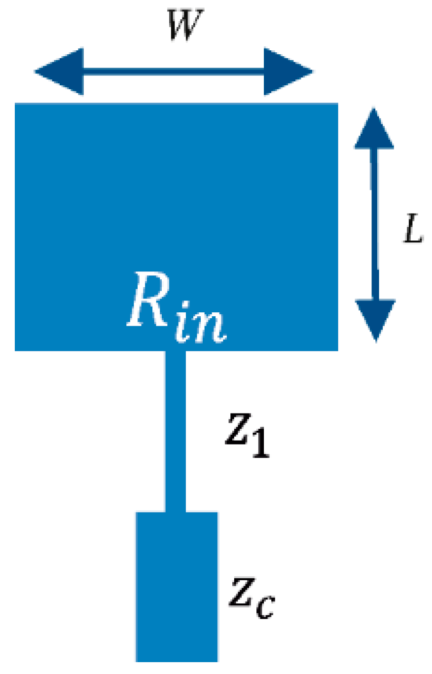
Length (L)	1.11	1.11	N/A	mm
Width (W)	1.52	1.52	N/A	mm
Notch width (g)	N/A	0.0084	N/A	mm
$\mathrm{Notch} \mathrm{depth} (y_0$)	N/A	0.15	N/A	mm
Quarter wave transformer patch
Parameter	Antenna 1	Antenna 2	Antenna 3	units
Transmission line Z1
Length (L)	0.726	N/A	0.935	mm
Width (W)	0.082	N/A	0.082	mm
Transmission line Zc
Length (L)	0.68	0.435	0.68	mm
Width (W)	0.37	0.37	0.37	mm
Lower quarter wave transformer
Parameter	Antenna 1	Antenna 2	Antenna 3	units
Rin lower position
Length (L)	0.68	0.68	0.68	mm
Width (W)	0.37	0.37	0.37	mm
Z1 lower position
Length (L)	0.705	0.705	0.705	mm
Width (W)	0.2	0.2	0.2	mm
Zc lower position
Length (L)	0.725	0.725	0.725	mm
Width (W)	0.082	0.082	0.082	mm
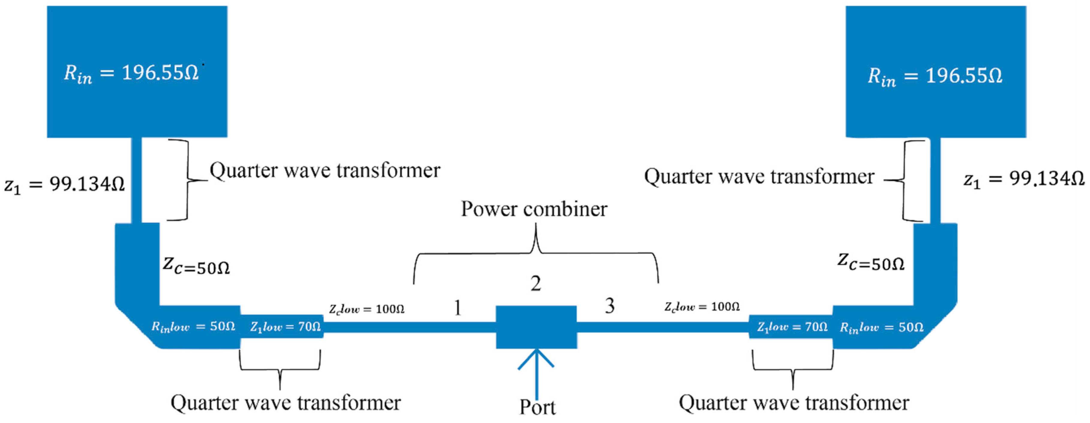
Power combiner
Parameter	Antenna 1	Antenna 2	Antenna 3	units
1
Length (L)	0.725	0.725	0.725	mm
Width (W)	0.082	0.082	0.082	mm
2
Length (L)	0.68	0.68	0.68	mm
Width (W)	0.37	0.37	0.37	mm
3
Length (L)	0.725	0.725	0.725	mm
Width (W)	0.082	0.082	0.082	mm

.

Figure 9a–c show the arrays of 32 ports for each type of designed antenna. These arrays were the largest ones that were simulated in each case.

The horizontal and vertical spacing between the array elements is λ (a wavelength unit), and, as previously stated, arrays of 1, 2, 4, 6, 8, 12, 16, and 32 elements were simulated to observe the evolution of the different parameters with the increase in elements.

Figure 10 depicts the behavior of return loss vs. frequency for each 16-element array, which present minimum values in the 60 GHz frequency. It can be noted that Antenna I (square patch with quarter-wave coupling) has a −23.8 dB value, Antenna II (square patch with inset feed) has −21.72 dB, and Antenna III (circular patch with quarter-wave coupling length) has −39.64 dB.

For 32-element antennas in Figure 9a–c, the return loss simulation is also presented in Figure 11. While values for Antennas I and II slightly change, a significant improvement is obtained for Antenna III in relation to 16-element arrays.

Figure 10 and Figure 11 are examples of the variation of an antenna parameter when the number of array elements is increased. However, the parameters of gain, directivity, beamwidth, radiation efficiency, bandwidth, and return loss have also been obtained for each simulated array. The VSWR (voltage standing wave ratio) value is found by means of the reflection coefficient ($\Gamma$) with Equation (26).

$$VSWR=\frac{1+\Gamma }{1-\Gamma }$$

(26)

In

Table 4. Estimated data for the development of antennas.

Square Patch Antenna with Coupling Length λ/4 (Antenna 1)
Parameter	Port 1	Port 2	Port 4	Port 6	Port 8	Port 12	Port 16	Port 32
Frequency (GHz)	60	60	60	60	60	60	60	60
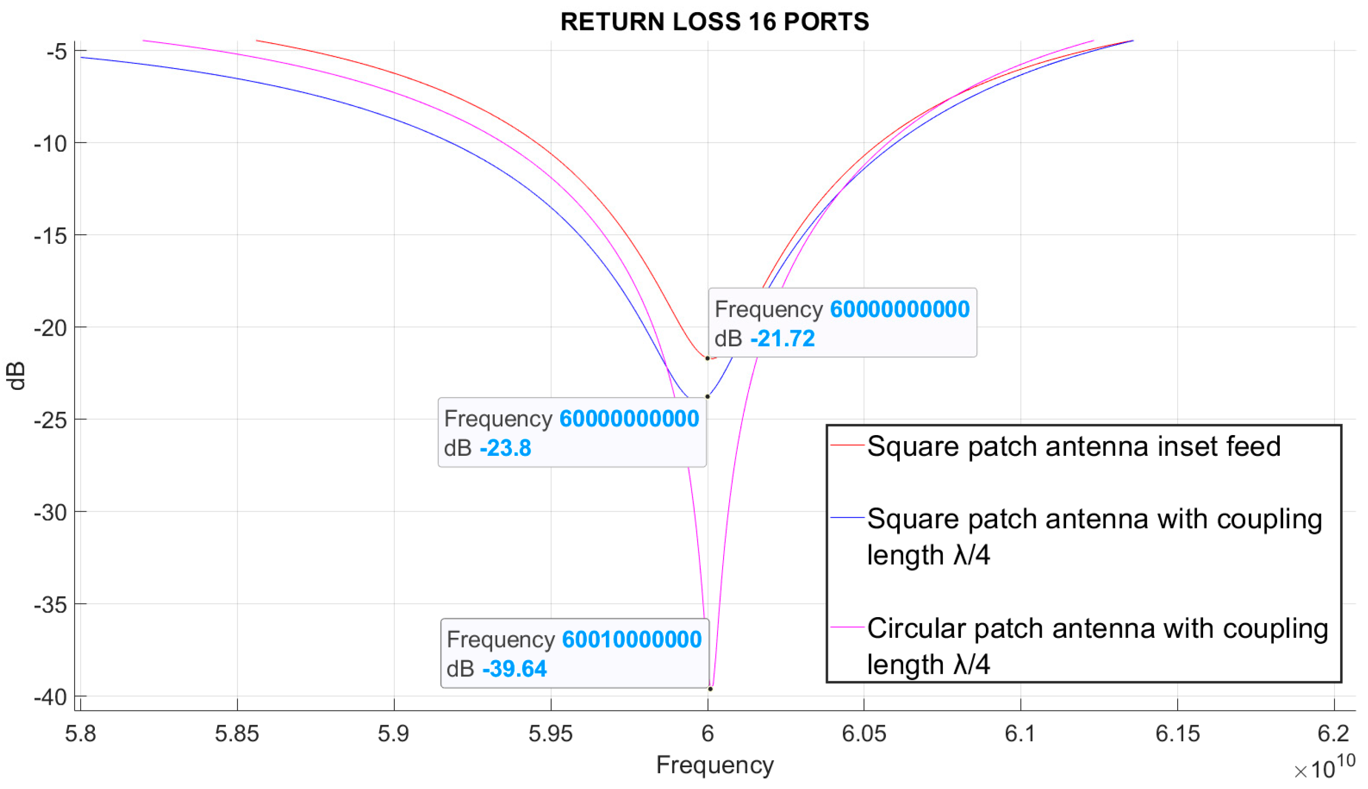
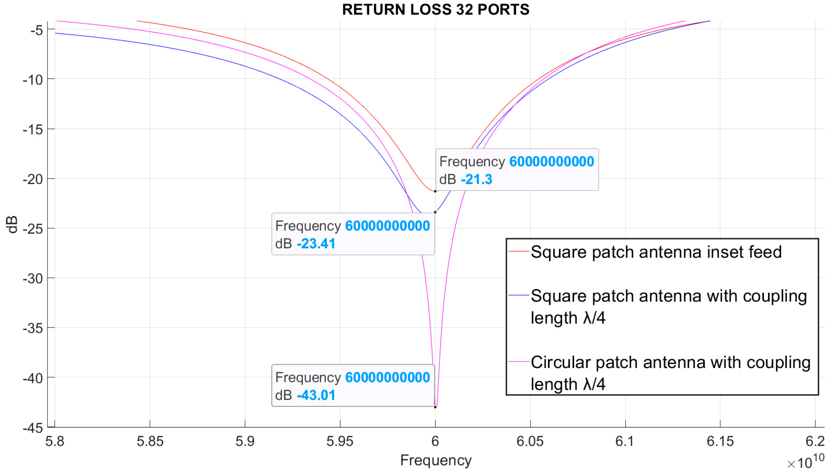
Return Loss (dB)	−24.542	−24.531	−24.174	−24.223	−24.211	−23.359	−23.795	−23.406
Bandwidth (GHz)	1.5	1.5	1.52	1.52	1.5	1.52	1.5	1.46
Gain (dBi)	8.42	11.654	14.325	16.102	17.326	18.959	20.02	23.335
Directivity (dBi)	10.861	13.802	16.726	18.509	19.798	21.734	23.096	26.305
Beamwidth (°)	22	10	10	6	4	4	4	4
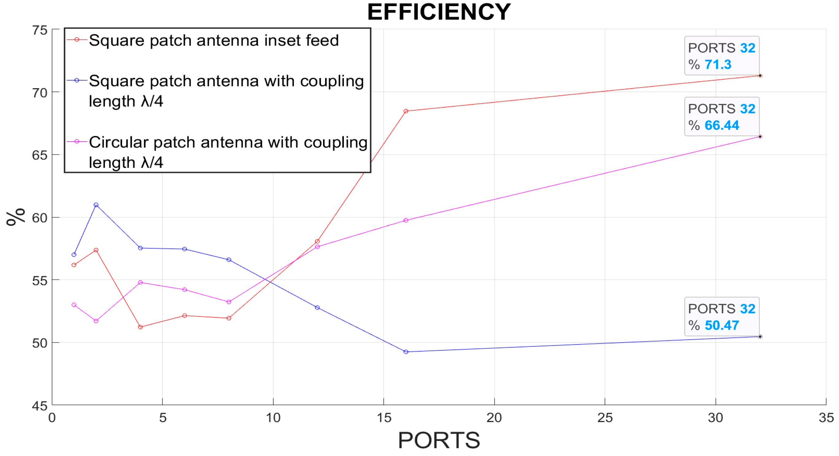
Antenna efficiency (%)	57.0033	60.9818	57.53075	57.4513	56.59786	52.7837	49.2493	50.4661
Square patch antenna with inset feed model (Antenna 2)
Parameter	Port 1	Port 2	Port 4	Port 6	Port 8	Port 12	Port 16	Port 32
Frequency (GHz)	60	60	60	60	60	60	60	60
Return Loss (dB)	−20.425	−20.475	−21.552	−21.575	−21.616	−21.312	−21.717	−21.301
Bandwidth (GHz)	1.46	1.18	1.18	1.16	1.16	1.16	1.15	1.15
Gain (dBi)	6.746	9.978	12.061	13.936	15.213	17.1865	19.028	22.176
Directivity (dBi)	9.25	12.391	14.966	16.764	18.058	19.5471	20.6732	23.645
Beamwidth (°)	20	10	10	6	4	4	4	4
Antenna efficiency (%)	56.18236	57.372	51.22713	52.1435	51.93977	58.0684	68.4668	71.3017
Circular patch antenna with coupling length λ/4 (Antenna 3)
Parameter	Port 1	Port 2	Port 4	Port 6	Port 8	Port 12	Port 16	Port 32
Frequency (GHz)	60	60	60	60	60	60	60	60
Return Loss (dB)	−35.722	−34.93	−36.424	−37.063	−36.833	−38.022	−39.643	−42.988
Bandwidth (GHz)	1.27	1.27	1.27	1.29	1.29	1.31	1.31	1.32
Gain (dBi)	8.104	11.012	14.233	16.049	17.291	19.57	20.984	24.541
Directivity (dBi)	10.861	13.876	16.846	18.708	20.029	21.963	23.221	26.317
Beamwidth (°)	22	10	10	6	6	6	6	6
Antenna efficiency (%)	53.00294	51.713	54.78984	54.2126	53.23534	57.6368	59.7448	66.4355

, it is observed that some parameters such as bandwidth and return loss vary less than others, such as gain, directivity, beamwidth, and efficiency when the number of ports is increased. Figure 12 shows the evolution of efficiency when the number of ports is increased.

According to Figure 12, Antenna I tends to reduce its efficiency when ports are increased, unlike Antennas II and III. Figure 12 displays that the inset feed coupling antenna (Antenna II) is the one with the highest efficiency when ports are increased, achieving a 5% difference above the circular antenna (Antenna III) when there are 32 ports. Besides, Antenna II is the smallest one since it does not have a quarter-wave transformer. From a broader perspective, Antennas I and III have similar directivity, higher than Antenna II directivity in all cases. In the case of 32-port antennas, Antenna I has a 26.305 dBi directivity, Antenna II has 23.645 dBi, and Antenna III has 26.317 dBi. This fact establishes that the high efficiency of Antenna II compensates for its low directivity, which is close to half the directivity of Antennas I and III (−3 dB, approximately). Therefore, Antenna II has the lowest gain in all cases, including the 32-port one (22.176 dBi). In this case, Antenna I has a gain of 23.33 dBi, whereas Antenna III has 24.41 dBi. In conclusion, the best antenna in terms of efficiency and gain performance is Antenna III.

Regarding return loss, Antenna III has also produced the best results, which enable it to couple to the transmitter more properly. Table 4 also presents that Antenna I has the highest bandwidth in all cases, followed by Antenna III. In the case of 32-port antennas, the bandwidth difference between Antennas I and III is 140 MHz, while the difference between Antennas I and II is 310 MHz. Half power beamwidth is lower for Antennas I and II, but it diminished in all antennas when ports were increased. After six ports, this reduction is very low.

4. Conclusions

Three types of MIMO microstrip antenna arrays were simulated to operate at a 60 GHz frequency between 1 and 30 ports with FR-4 substrate. After the simulation, it can be noted that increasing the number of ports in the MIMO array also increases some parameters, such as directivity and gain, while others, such as bandwidth and return loss, are relatively constant.

From the three antennas that were used in the experiment, the circular patch antenna with quarter-wave coupling (Antenna III) shows the best performance in terms of return loss and gain. In the 32-port case, Antenna III gain was approximately 2 dB above Antenna II, and 1 dB above Antenna I. The difference in terms of return loss between Antenna III and Antennas I and II was over 10 dB for 32-port antennas, which indicates a better radio coupling. Regarding efficiency, Antenna III places second, 5% below the Antenna II performance in the 32-port array.

The square patch antenna with quarter-wave coupling (Antenna I) has the highest bandwidth. It shows a 140 MHz bandwidth higher than Antenna III, and 310 MHz higher than Antenna II, which can be useful depending on its application.

This article also contains a rapid prototyping method that helps to reduce times, especially when each array requires specific coordinates on the ADS software to respect design dimensioning. When considering the number of built and simulated arrays, rapid prototyping is highly helpful to develop these tests.

References

- Mehta, A.; Ramer, R.; Gong, L.; Sachdeva, S. H-shaped microstrip antenna for broadband communications at 60 GHz. In Proceedings of the 2015 IEEE Asia Pacific Conference on Postgraduate Research in Microelectronics and Electronics (PrimeAsia), Hyderabad, India, 27–29 November 2015; pp. 80–82. [Google Scholar] [CrossRef]
- Jackson, D.R.; Long, S.A. History of Microstrip and Dielectric Resonator Antennas. In Proceedings of the 2020 14th European Conference on Antennas and Propagation (EuCAP), Copenhagen, Denmark, 15–20 March 2020; pp. 1–5. [Google Scholar] [CrossRef]
- Schulz, B. 802.11ad—WLAN at 60 GHz A Technology Introduction. Rohde & Schwarz, 2017. Available online: https://scdn.rohde-schwarz.com/ur/pws/dl_downloads/dl_application/application_notes/1ma220/1MA220_3e_WLAN_11ad_WP.pdf (accessed on 22 November 2021).
- Luis, A.M.; Andrés, M.A.; Luis, S.V.; Miguel, B. “Diseño e Implementación de Antena Microstrip,” IX Congreso De Microelectrónica Aplicada (UEA) 2018. 2018. Available online: http://latics.tecno.unca.edu.ar/ocs/index.php/uea2018/uea2018/schedConf/presentations (accessed on 25 November 2021).
- Imtiaj, S.; Bhattacharya, S. Performance Comparison between 2×1 and 2×2 Corporate Feed Antenna Array in X-band. In Proceedings of the 2020 IEEE Calcutta Conference (CALCON), Kolkata, India, 28–29 February 2020; pp. 189–193. [Google Scholar] [CrossRef]
- Lahmadi, S.; Tahar, J.B.H. Optimization of 60 GHz MIMO antenna by adding ground stub to reduce mutual coupling for WPAN applications. In Proceedings of the 2017 25th International Conference on Software, Telecommunications and Computer Networks (SoftCOM), Split, Croatia, 21–23 September 2017; pp. 1–4. [Google Scholar] [CrossRef]
- Estupiñan Cuesta, E.P.; Martínez Quintero, J.C.; Rugeles Uribe, J.J. Metodología de diseño de antenas microstrip por caracterización del dieléctrico. In Proceedings of the 14th Congreso Internacional de Electrónica Control y Telecomunicaciones, Bogotá, Colombia, 18–19 November 2019; Universidad Distrital Francisco Jose de caldas: Bogotá, Colombia, 2019; Volume 13, ISBN 978-958-44-5254-2. [Google Scholar]
- Sipal, D.; Abegaonkar, M.P.; Koul, S.K. Compact Planar 3.5/5.5 GHz Dual Band MIMO USB Dongle Antenna for WiMAX Applications. In Proceedings of the 2018 IEEE Indian Conference on Antennas and Propogation (InCAP), Hyderabad, India, 16–19 December 2018; pp. 1–4. [Google Scholar] [CrossRef]
- Mishra, M.; Chaudhuri, S.; Kshetrimayum, R.S. Low Mutual Coupling Four-Port MIMO Antenna Array for 3.5 GHz WiMAX Application. In Proceedings of the 2020 IEEE Region 10 Symposium (TENSYMP), Dhaka, Bangladesh, 5–7 June 2020; pp. 791–794. [Google Scholar] [CrossRef]
- Hakim, M.L.; Uddin, M.J.; Hoque, M.J. 28/38 GHz Dual-Band Microstrip Patch Antenna with DGS and Stub-Slot Configurations and Its 2×2 MIMO Antenna Design for 5G Wireless Communication. In Proceedings of the 2020 IEEE Region 10 Symposium (TENSYMP), Dhaka, Bangladesh, 5–7 June 2020; pp. 56–59. [Google Scholar] [CrossRef]
- Hasan, M.N.; Seo, M. Compact Omnidirectional 28 GHz 2×2 MIMO Antenna Array for 5G Communications. In Proceedings of the 2018 International Symposium on Antennas and Propagation (ISAP), Busan, Korea, 23–26 October 2018; pp. 1–2. [Google Scholar]
- Naik, M.N.; Virani, H.A. High Gain 16 Ports MIMO Antenna at 60 GHz for Millimeter Wave Applications. In Proceedings of the 2019 IEEE Indian Conference on Antennas and Propogation (InCAP), Ahmedabad, India, 19–22 December 2019; pp. 1–3. [Google Scholar] [CrossRef]
- Nurrachman, M.; Hakim, G.P.N.; Firdausi, A. Design of Rectangular Patch Array 1×2 MIMO Microstrip Antenna with Tapered Peripheral Slits Method for 28 GHz Band 5G mmwave Frequency. In Proceedings of the 2020 2nd International Conference on Broadband Communications, Wireless Sensors and Powering (BCWSP), Yogyakarta, Indonesia, 28–30 September 2020; pp. 16–20. [Google Scholar] [CrossRef]
- Pant, M.; Malviya, L.; Choudhary, V. Gain and Bandwidth Enhancement of 28 GHz Tapered Feed Antenna Array. In Proceedings of the 2020 11th International Conference on Computing, Communication and Networking Technologies (ICCCNT), Kharagpur, India, 1–3 July 2020; pp. 1–4. [Google Scholar] [CrossRef]
- Chandra, R.; Sarkar, D.; Ganguly, D.; Saha, C.; Siddiqui, J.Y.; Antar, Y.M.M. Design of NFRP Based SIR-Loaded Two Element MIMO Antenna System for 28/38 GHz sub mm-wave 5G Applications. In Proceedings of the 2020 IEEE 3rd 5G World Forum (5GWF), Bangalore, India, 10–12 September 2020; pp. 514–518. [Google Scholar] [CrossRef]
- Ullah, H.; Tahir, F.A. An Asymmetric Semi-circular Meandered Line Monopole Antenna for 28 GHz 5G Communications. In Proceedings of the 2020 International Conference on UK-China Emerging Technologies (UCET), Glasgow, UK, 20–21 August 2020; pp. 1–3. [Google Scholar] [CrossRef]
- Liu, P.; Zhu, X.-W.; Zhang, Y.; Wang, X.; Yang, C.; Jiang, Z.H. Patch Antenna Loaded with Paired Shorting Pins and H-Shaped Slot for 28/38 GHz Dual-Band MIMO Applications. IEEE Access 2020, 8, 23705–23712. [Google Scholar] [CrossRef]
- Jose, M.C.; Radha, S.; Sreeja, B.S.; Kumar, P. Design of 28 GHz High Gain 5G MIMO Antenna Array System. In Proceedings of the TENCON 2019—2019 IEEE Region 10 Conference (TENCON), Kochi, India, 7–10 December 2021; pp. 1913–1916. [Google Scholar] [CrossRef]
- Yang, C.; Hsu, C.; Hwang, L. Millimeter Wave Dual Polarization Design Using Frequency Selective Surface (FSS) for 5G Base-Station Applications. In Proceedings of the 2019 IEEE 69th Electronic Components and Technology Conference (ECTC), Las Vegas, NV, USA, 28–31 May 2019; pp. 2200–2205. [Google Scholar] [CrossRef]
- Yuwono, T.; Ismail, M.; Hajar, I. Design of Massive MIMO for 5G 28 GHZ. In Proceedings of the 2019 2nd International Conference on Computer Applications & Information Security (ICCAIS), Riyadh, Saudi Arabia, 19–21 March 2019; pp. 1–4. [Google Scholar] [CrossRef]
- ADS. PathWave Advanced Design System. Available online: https://www.keysight.com/zz/en/products/software/pathwave-design-software/pathwave-advanced-design-system.html (accessed on 21 November 2021).
- Balanis, C.A. Antenna Theory: Analysis and Design; John Wiley & Sons Inc.: Hoboken, NJ, USA, 2016; pp. 783–867. [Google Scholar]
- Li, M.; Jamal, M.Y.; Li, X.; Yeung, K.L.; Jiang, L.; Itoh, T.; Murch, R. A Millimeter-Wave Frequency-Reconfigurable Fabry–Pérot Cavity Antenna. IEEE Antennas Wirel. Propag. Lett. 2022, 21, 1537–1541. [Google Scholar] [CrossRef]
- Amir, N.A.; Hamzah, S.A.; Ramli, K.N.; Esa, M. 2×1 microstrip patch array antenna with harmonic suppression capability. In Proceedings of the 2016 IEEE Asia-Pacific Conference on Applied Electromagnetics (APACE), Langkawi, Malaysia, 11–13 December 2016; pp. 272–276. [Google Scholar] [CrossRef]
- Bancroft, R. Microstrip and Printed Antenna Design, 2nd ed.; Scitech Publishing: Boulder, Colorado, 2009; pp. 10–56. [Google Scholar]
- Pozar, D. Microwave Engineering, 4th ed.; John Wiley & Sons, Inc.: Amherst, MA, USA, 2012; pp. 147–153. [Google Scholar]