

Hawaiian Treeline Ecotones: Implications for Plant Community Conservation under Climate Change

Abstract
:1. Introduction
2. Results
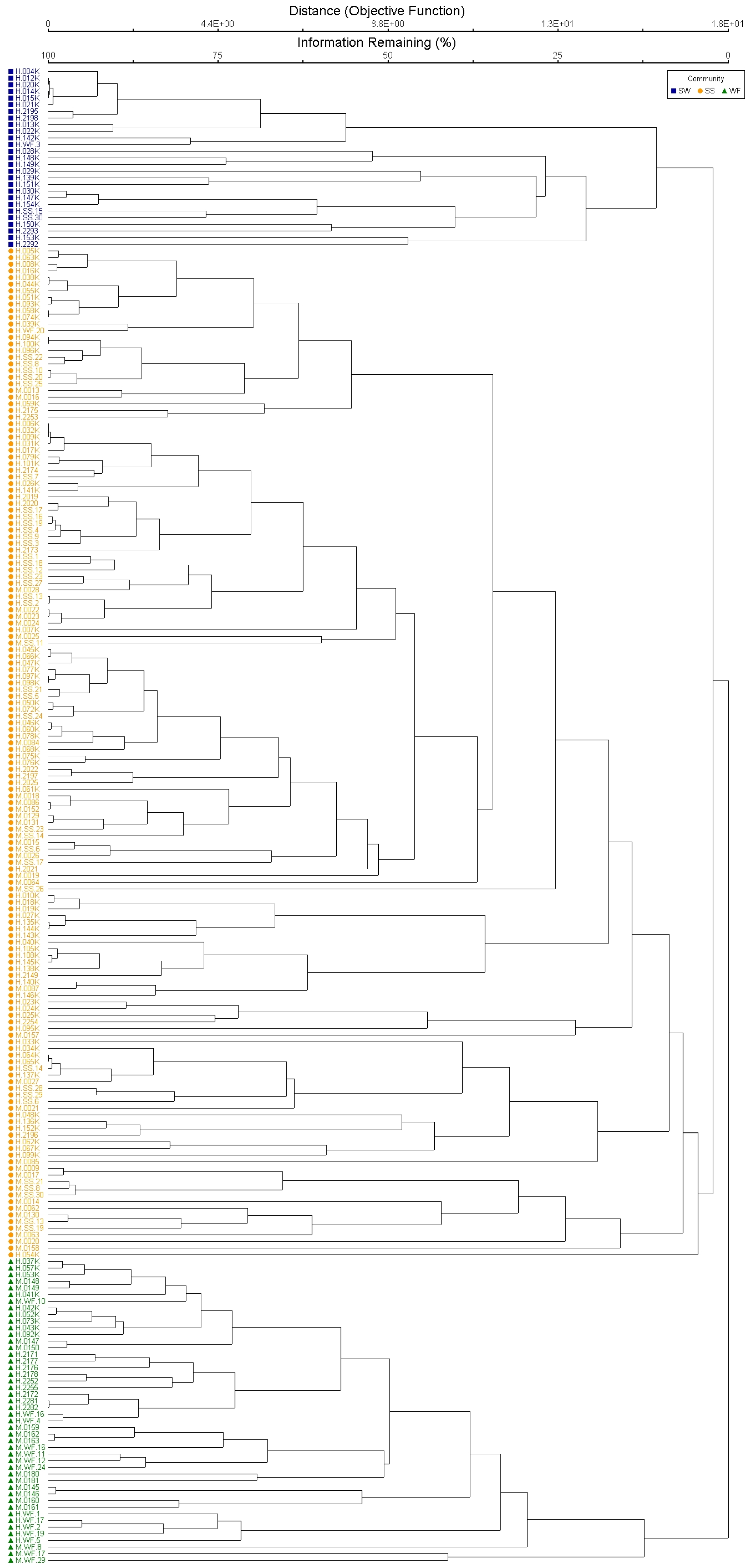
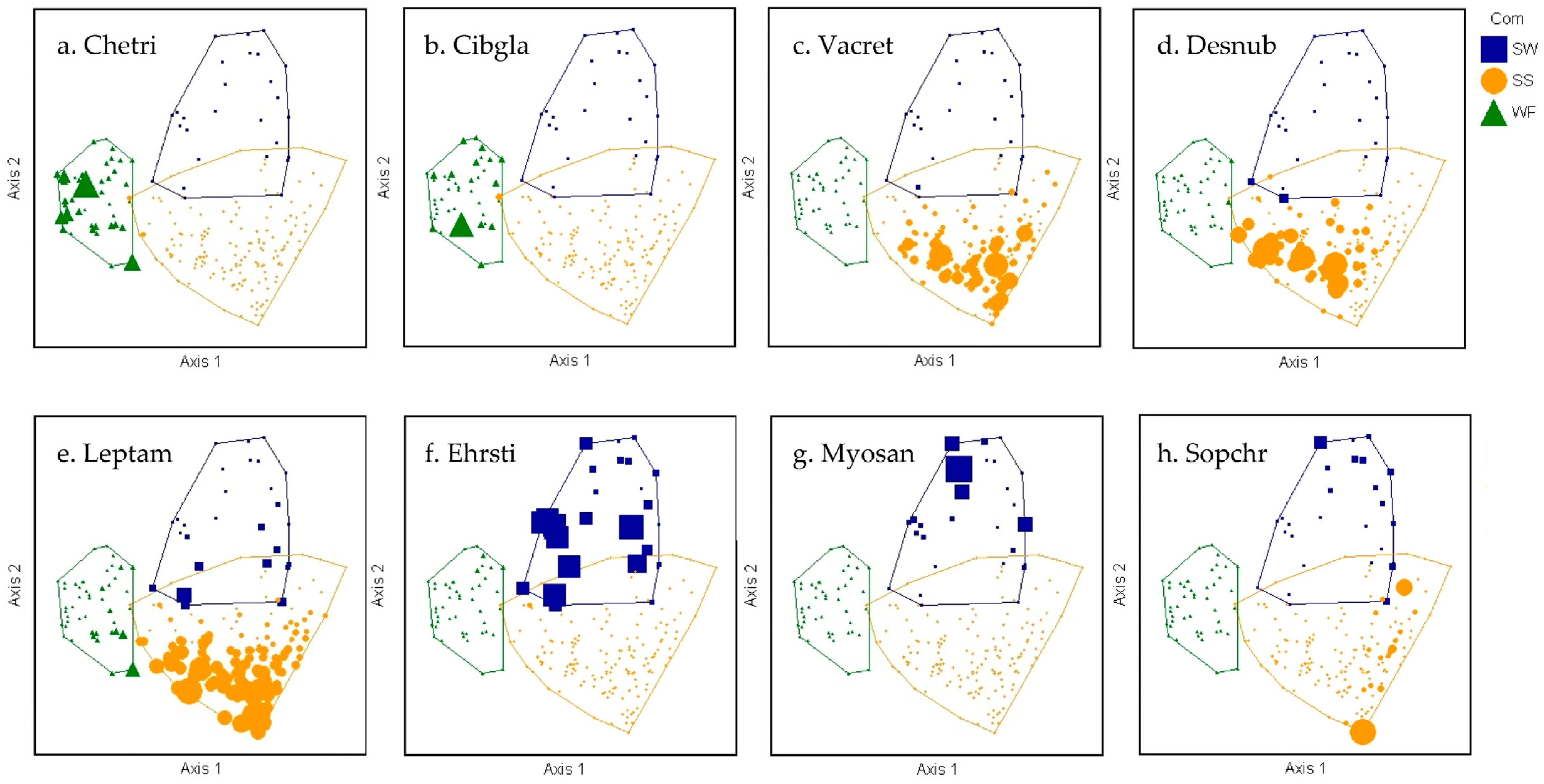
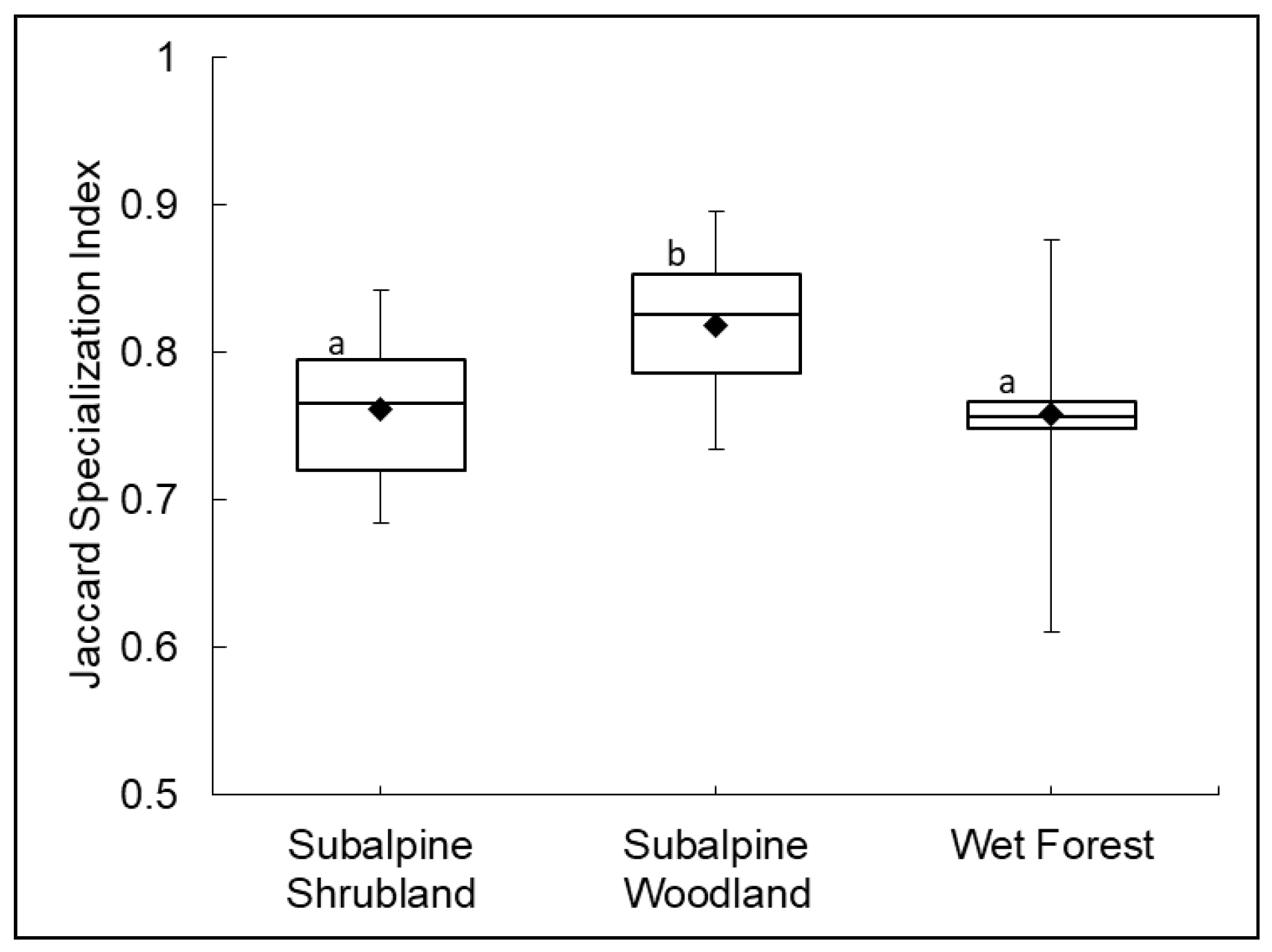
2.1. Plant Community Composition

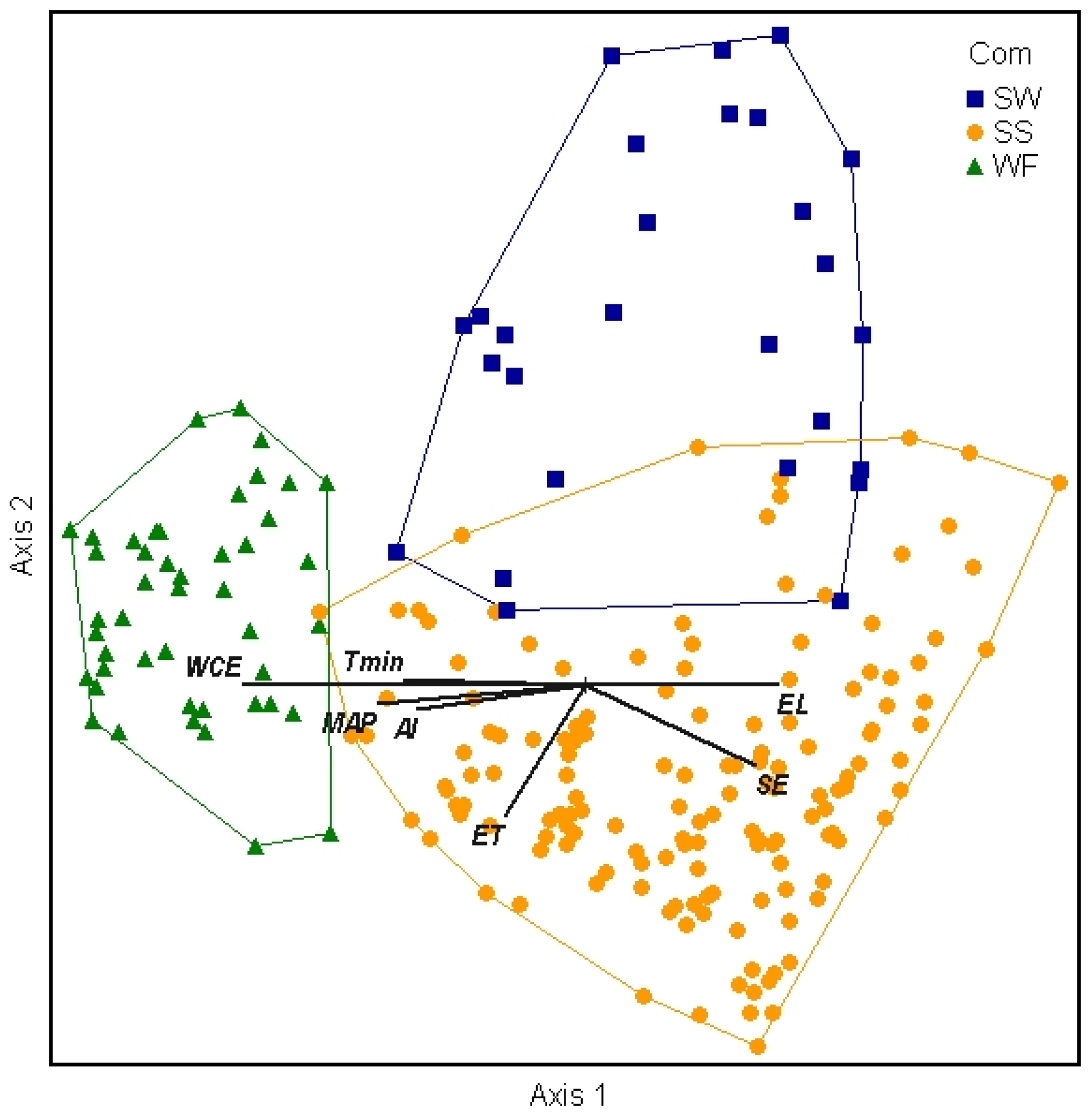
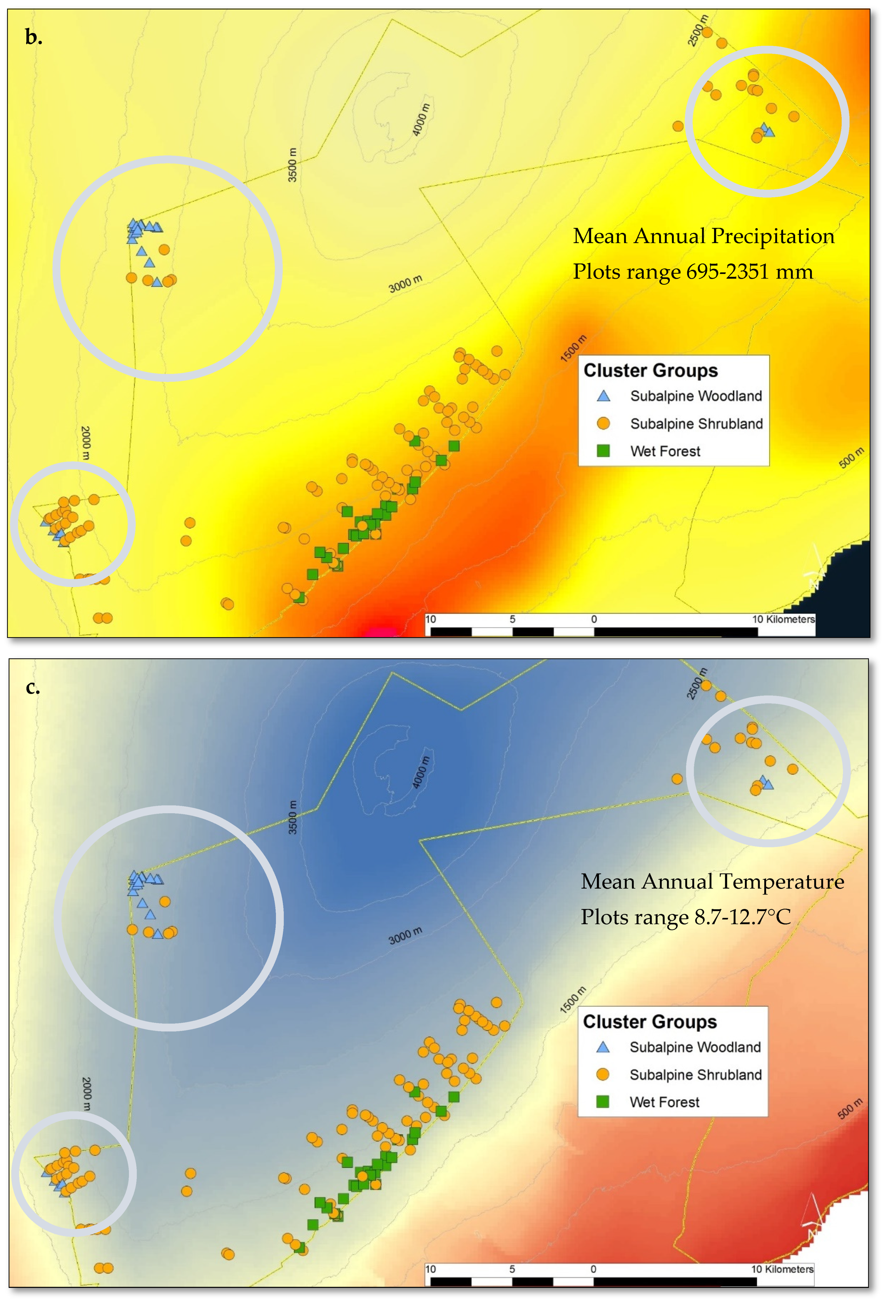
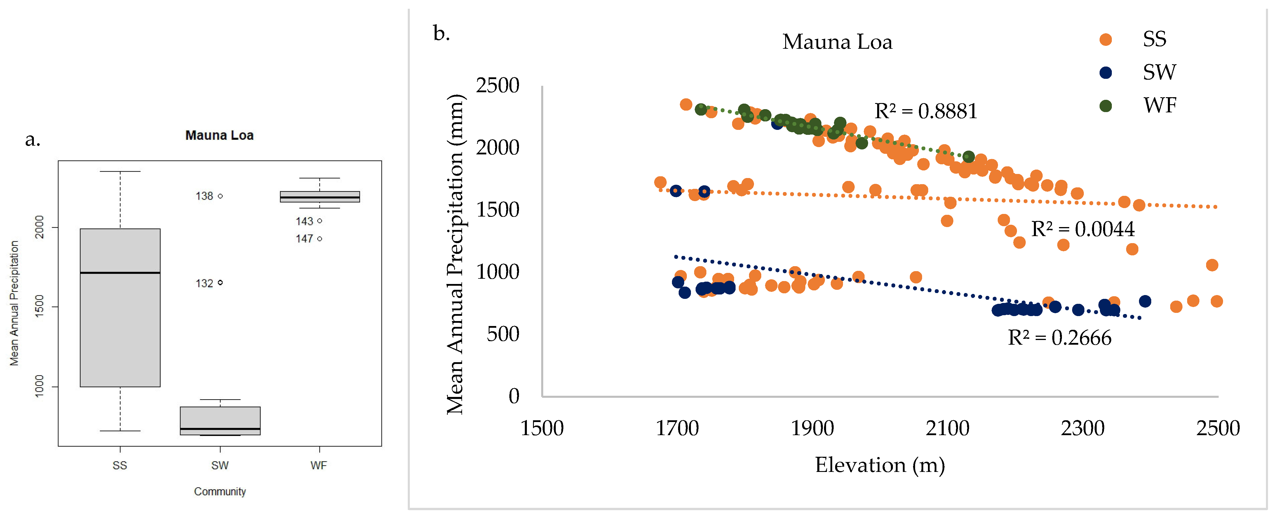
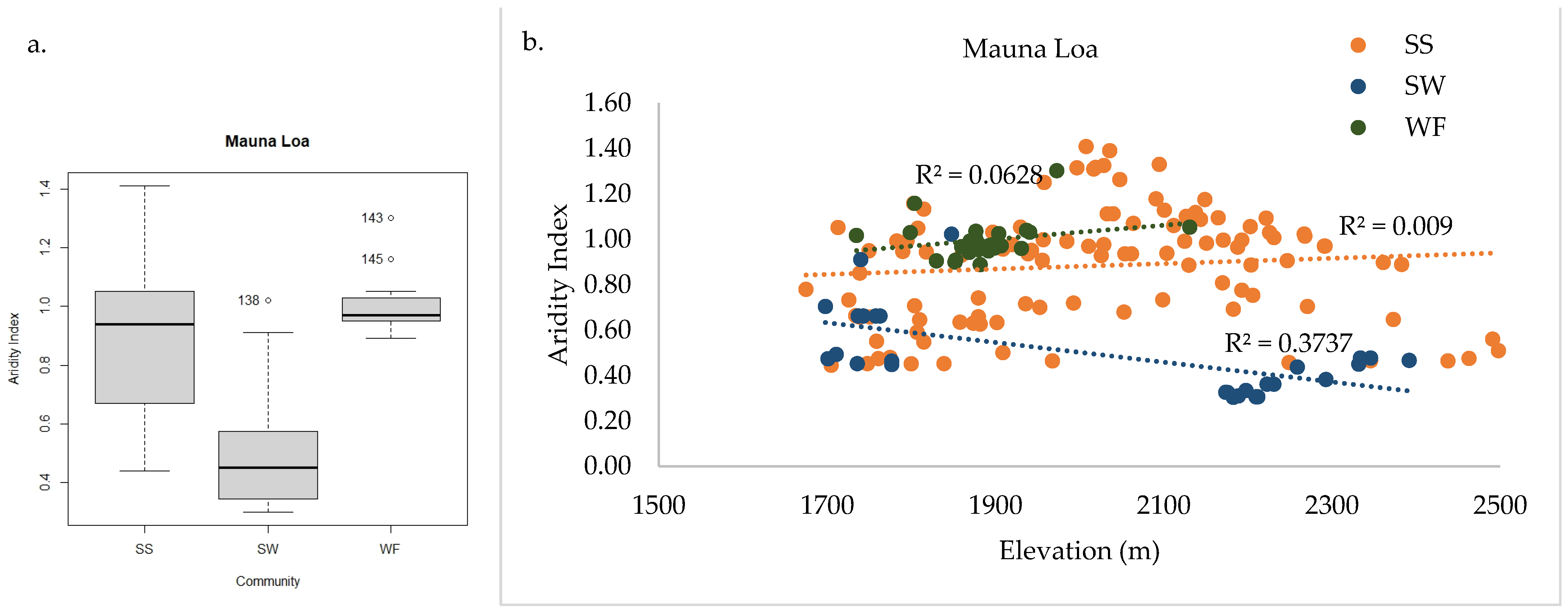
2.2. Plant Community–Environment Correlations
2.3. Site-Specific Patterns
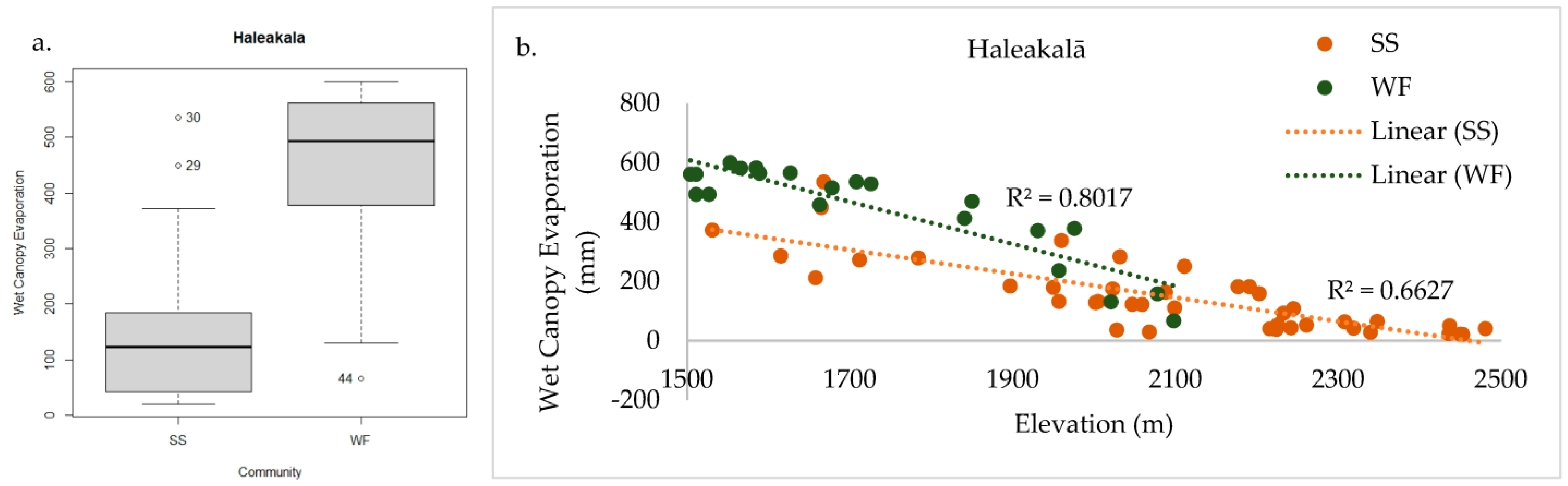
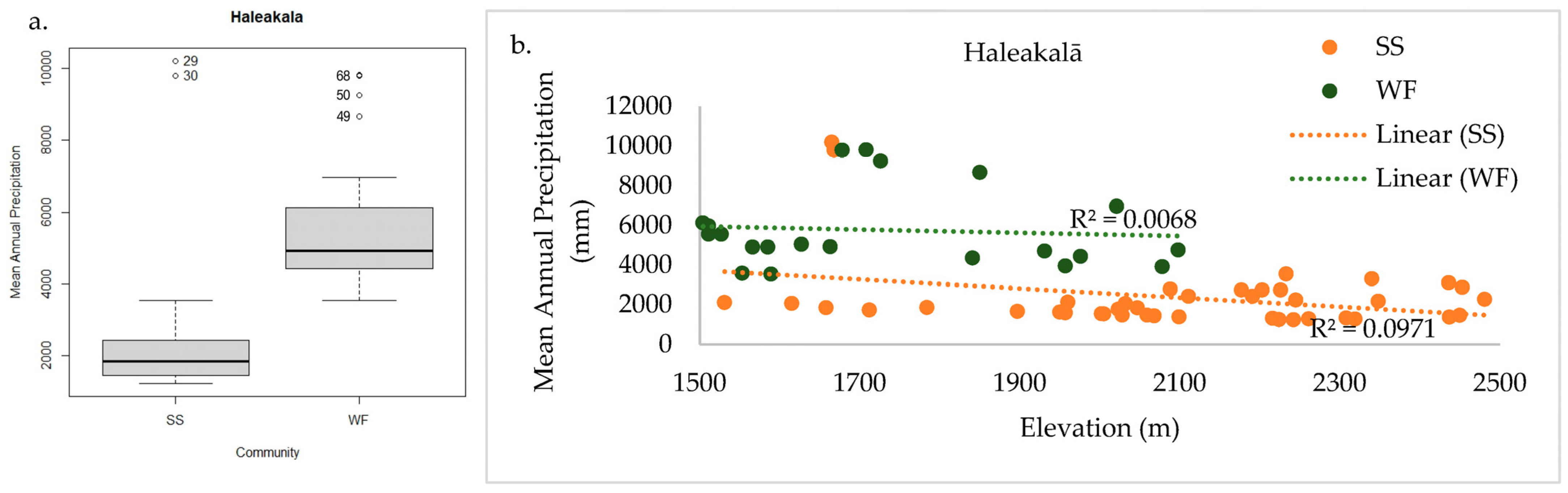
2.3.1. Haleakalā
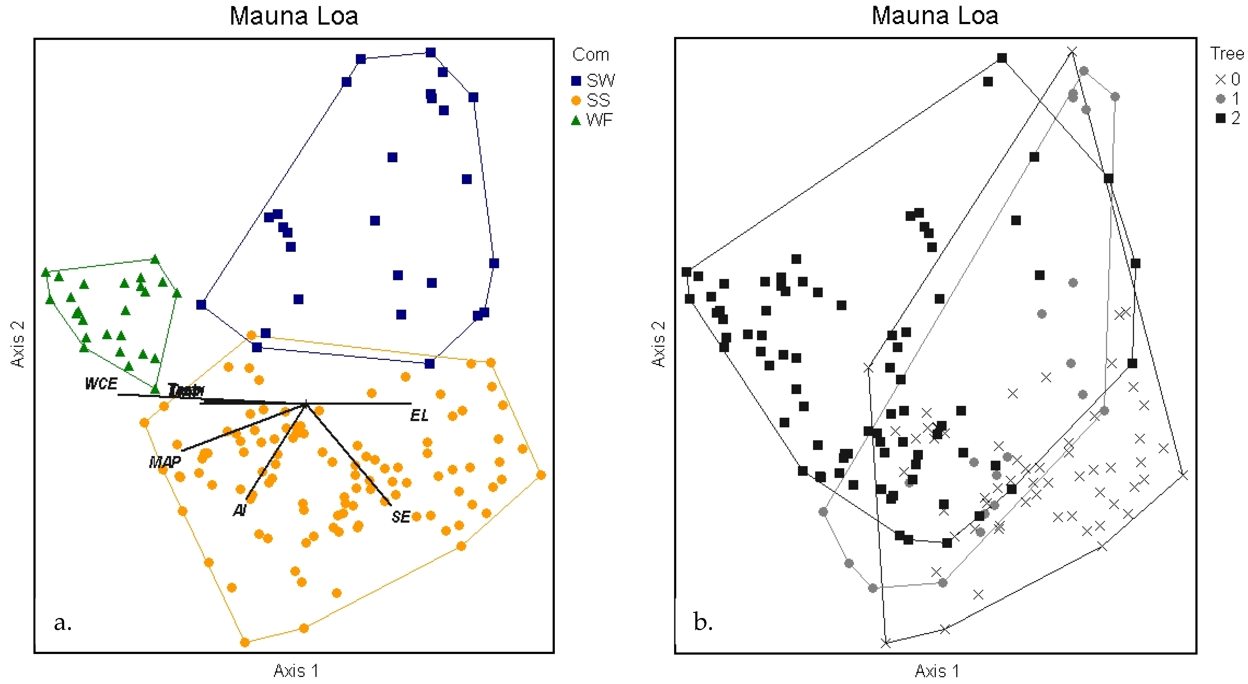
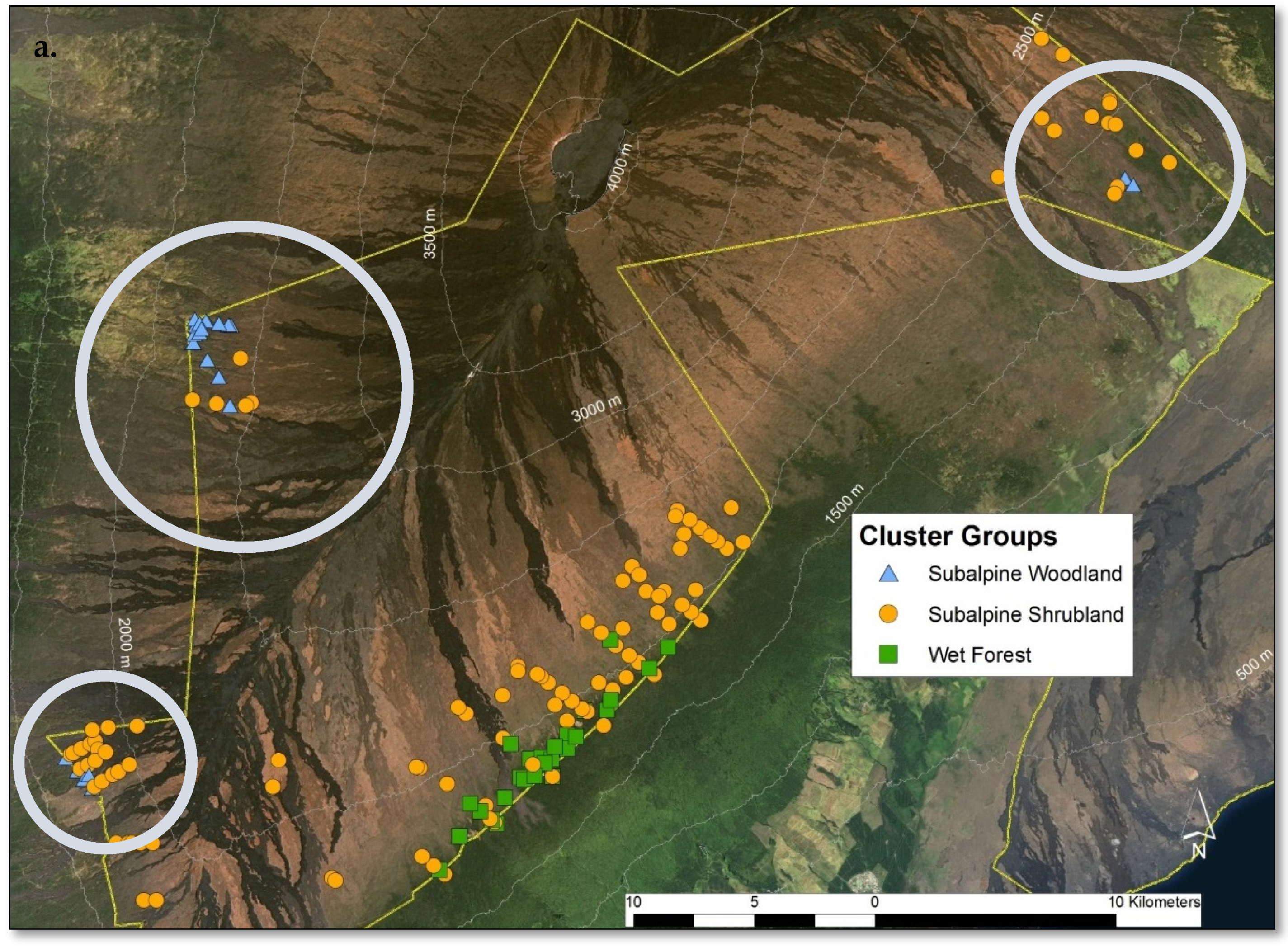
2.3.2. Mauna Loa
3. Discussion
3.1. Treeline Ecotone Composition and Structure
3.1.1. Wet Forest
3.1.2. Subalpine Shrubland
3.1.3. Subalpine Woodland
3.2. Environmental Drivers
4. Materials and Methods
5. Conclusions
Supplementary Materials
Author Contributions
Funding
Data Availability Statement
Acknowledgments
Conflicts of Interest
References
- Körner, C. Alpine Treelines; Springer: Basel, Switzerland, 2012. [Google Scholar]
- Körner, C. Alpine Plant Life: Functional Plant Ecology of High Mountain Ecosystems; Springer: Berlin/Heidelberg, Germany, 2003. [Google Scholar]
- Körner, C.; Paulsen, J. A world-wide study of high altitude treeline temperatures. J. Biogeogr. 2004, 31, 713–732. [Google Scholar] [CrossRef]
- Leuschner, C. Timberline and alpine vegetation on the tropical and warm-temperate oceanic islands of the world: Elevation, structure and floristics. Vegetatio 1996, 123, 193–206. [Google Scholar] [CrossRef]
- Williams, J.W.; Jackson, S.T.; Kutzback, J.E. Projected distributions of novel and disappearing climates by 2100 AD. Proc. Natl. Acad. Sci. USA 2007, 104, 5738–5742. [Google Scholar] [CrossRef] [PubMed]
- Wardle, P. An explanation for alpine timberline. N. Z. J. Botan. 1971, 9, 371–402. [Google Scholar] [CrossRef]
- Whittaker, R.J.; Fernández-Palacios, J.M. Island Biogeography: Ecology, Evolution, and Conservation; Oxford University Press: Oxford, UK, 2007. [Google Scholar]
- Karger, D.N.; Kessler, M.; Conrad, O.; Weigelt, P.; Kreft, H.; Konig, C.; Zimmermann, N. Why tree lines are lower on islands—Climatic and biogeographic effects hold the answer. Glob. Ecol. Biogeogr. 2019, 28, 839–850. [Google Scholar] [CrossRef]
- MacArthur, R.H.; Wilson, E.O. The Theory of Island Biogeography; Princeton University Press: Princeton, NJ, USA, 1967. [Google Scholar]
- Kitayama, K. Patterns of species diversity on an oceanic versus a continental island mountain: A hypothesis on species diversification. J. Veg. Sci. 1996, 7, 879–888. [Google Scholar] [CrossRef]
- Crausbay, S.D.; Frazier, A.G.; Giambelluca, T.W.; Longman, R.J.; Hotchkiss, S.C. Moisture status during a strong El Niño explains a tropical montane cloud forest’s upper limit. Oecologia 2014, 175, 273–284. [Google Scholar] [CrossRef]
- Crausbay, S.D.; Martin, P.H.; Kelly, E.F. Tropical montane vegetation dynamics near the upper cloud belt strongly associated with a shifting ITCZ and fire. J. Ecol. 2015, 103, 891–903. [Google Scholar] [CrossRef]
- Irl, S.D.H. Plant diversity on high elevation islands—Drivers of species richness and endemism. Front. Biogeogr. 2016, 8, e29717. [Google Scholar] [CrossRef]
- Irl, S.D.H.; Anthelme, F.; Harter, D.E.V.; Jentsch, A.; Lotter, E.; Steinbauer, M.J.; Beierkuhnlein, C. Patterns of island treeline elevation—A global perspective. Ecography 2016, 39, 427–436. [Google Scholar] [CrossRef]
- Brito, P.; Wieser, G.; Oberhuber, W.; Gruber, A.; Lorenzo, J.R.; González-Rodríguez, Á.M.; Jimenez, M.S. Water availability drives stem growth and stem water deficit of Pinus canariensis in a drought-induced treeline in Tenerife. Plant Ecology 2017, 218, 277–290. [Google Scholar] [CrossRef]
- Rehm, E.M.; Feeley, K.J. Freezing temperatures as a limit to forest recruitment above tropical Andean treelines. Ecology 2015, 96, 1856–1865. [Google Scholar] [CrossRef]
- Harsch, M.A.; Hulme, P.E.; McGlone, M.S.; Duncan, R.P. Are treelines advancing? A global meta-analysis of treeline response to climate warming. Ecol. Lett. 2009, 12, 1040–1049. [Google Scholar] [CrossRef] [PubMed]
- Holtmeier, F.-K.; Broll, G. Treeline research—From the roots of the past to present time. A review. Forests 2020, 11, 38. [Google Scholar] [CrossRef]
- Camarero, J.J.; Gazol, A.; Sánchez-Salguero, R.; Fajardo, A.; McIntire, E.J.B.; Gutiérrez, E.; Batllori, E.; Boudreau, S.; Carrer, M.; Diez, J.; et al. Global fading of the temperature-growth coupling at alpine and polar treelines. Glob. Chang. Biol. 2021, 27, 1879–1889. [Google Scholar] [CrossRef] [PubMed]
- Feeley, K.J.; Silman, M.R.; Duque, A. Where are the tropical plants? A call for better inclusion of tropical plants in studies investigating and predicting the effects of climate change. Front. Biogeogr. 2015, 7, 174–176. [Google Scholar]
- Lenoir, J.; Svenning, J.-C. Climate-related range shifts—A global multidimensional synthesis and new research directions. Ecography 2015, 38, 15–28. [Google Scholar] [CrossRef]
- Naccarella, A.; Morgan, J.W.; Cutler, S.C.; Venn, S.E. Alpine treeline ecotone stasis in the face of recent climate change and disturbance by fire. PLoS ONE 2020, 15, e0231339. [Google Scholar] [CrossRef]
- Lutz, D.A.; Powell, R.L.; Silman, M.R. Four decades of Andean timberline migration and implications for biodiversity loss with climate change. PLoS ONE 2013, 8, e74496. [Google Scholar] [CrossRef]
- Harsch, M.A.; Bader, M.Y. Treeline form—A potential key to understanding treeline dynamics. Glob. Ecol. Biogeogr. 2011, 20, 582–596. [Google Scholar] [CrossRef]
- Lett, S.; Dorrepaal, E. Global drivers of tree seedling establishment at alpine treelines in a changing climate. Funct. Ecol. 2018, 32, 1666–1680. [Google Scholar] [CrossRef]
- Holtmeier, F.-K. Mountain timberlines—Ecology, patchiness, and dynamics. In Advances in Global Change Research; Springer: Dordrecht, The Netherlands, 2009; Volume 36. [Google Scholar]
- Wiegand, T.; Camarero, J.J.; Rüger, N.; Gutiérrez, E. Abrupt population changes in treeline ecotones along smooth gradients. J. Ecol. 2006, 94, 880–892. [Google Scholar] [CrossRef]
- Martínez, I.; Wiegand, T.; Camarero, J.J.; Batllori, E.; Gutiérrez, E. Disentangling the formation of contrasting tree-line physiognomies combining model selection and Bayesian parameterization for simulation models. Am. Nat. 2011, 177, E136–E152. [Google Scholar] [CrossRef] [PubMed]
- Gagne, W.C.; Cuddihy, L.W. Vegetation. In Manual of Flowering Plants of Hawaii; Wagner, W.L., Herbst, D.H., Sohmer, S.H., Eds.; Bernice P. Bishop Museum: Honolulu, HI, USA, 1990; pp. 45–114. [Google Scholar]
- McCune, B.; Mefford, M.J. PC-ORD. Multivariate Analysis of Ecological Data, Version 6.08; MjM Software: Gleneden Beach, OR, USA, 2011.
- Kruskal, J.B. Nonmetric multidimensional scaling: A numerical method. Psychometrika 1964, 29, 115–129. [Google Scholar] [CrossRef]
- Mather, P.M. Computational Methods of Multivariate Analysis in Physical Geography; J. Wiley and Sons: London, UK, 1976. [Google Scholar]
- Dufrene, M.; Legendre, P. Species assemblages and indicator species: The need for a flexible asymmetrical approach. Ecol. Monogr. 1997, 67, 345–366. [Google Scholar] [CrossRef]
- Ainsworth, A.; Drake, D.R. Classifying Hawaiian plant species along a habitat generalist-specialist continuum: Implications for species conservation under climate change. PLoS ONE 2020, 15, e0228573. [Google Scholar] [CrossRef] [PubMed]
- Wagner, W.L.; Herbst, D.R.; Sohmer, S.H. Manual of the Flowering Plants of Hawaii, 2nd ed; University of Hawaii Press and Bishop Museum Press: Honolulu, HI, USA, 1999. [Google Scholar]
- Palmer, D.D. Hawaii’s Ferns and Fern Allies; University of Hawaii Press: Honolulu, HI, USA, 2003. [Google Scholar]
- Drake, D.R.; Mueller-Dombois, D. Population development of rain forest trees on a chronosequence of Hawaiian lava flows. Ecology 1993, 74, 1012–1019. [Google Scholar] [CrossRef]
- Benzing, D.H. Vulnerabilities of tropical forests to climate change: The significance of resident epiphytes. Clim. Chang. 1998, 39, 519–540. [Google Scholar] [CrossRef]
- Nadkarni, N.M.; Solano, R. Potential effects of climate change on canopy communities in a tropical cloud forest: An experimental approach. Oecologia 2002, 131, 580–586. [Google Scholar] [CrossRef]
- Pouteau, R.; Meyer, J.-Y.; Blanchard, P.; Nitta, J.H.; Terorotua, M.; Taputuarai, R. Fern species richness and abundance are indicators of climate change on high-elevation islands: Evidence from an elevational gradient on Tahiti (French Polynesia). Clim. Chang. 2016, 138, 143–158. [Google Scholar] [CrossRef]
- Daehler, C.C. Upper-montane plant invasions in the Hawaiian Islands: Patterns and opportunities. Perspect. Plant Ecol. Evol. Syst. 2005, 7, 203–216. [Google Scholar] [CrossRef]
- Simon, M.; Gross, J.; Ainsworth, A. Established Invasive Plant Species Monitoring: Hawai’i Volcanoes National Park; National Park Service: Fort Collins, CO, USA, 2016; Report No. NPS/PACN/NRR-2016/1202. [Google Scholar]
- Ainsworth, A.; Drake, D.R. Hawaiian subalpine plant communities: Implications for climate change. Pac. Sci. 2023; in press. [Google Scholar]
- Rehm, E.M.; Yelenik, S.; D’Antonio, C. Freezing temperatures restrict woody plant recruitment and restoration efforts in abandoned montane pastures. Glob. Ecol. Conserv. 2021, 26, e01462. [Google Scholar] [CrossRef]
- Green, K.; Hall, M.; Lopez, C.; Ainsworth, A.; Selvig, M.; Akamine, K.; Fugate, S.; Schulz, K.; Benitez, D.; Wasser, M.; et al. Vegetation Mapping Inventory Project: Hawaii Volcanoes National Park; National Park Service: Fort Collins, CO, USA, 2015; p. 316, Report No. NPS/PACN/NRR-2015/966. [Google Scholar]
- Green, K.; Schulz, K.; Lopez, C.; Ainsworth, A.; Selvig, M.; Akamine, K.; Meston, C.; Mallinson, J.W.; Urbanski, E.; Fugate, S.; et al. Vegetation Mapping Inventory Project: Haleakala National Park; National Park Service: Fort Collins, CO, USA, 2015; p. 297, Report No. NPS/PACN/NRR-2015/986. [Google Scholar]
- McDaniel, S.; Ostertag, R. Strategic light manipulation as a restoration strategy to reduce alien grasses and encourage native regeneration in Hawaiian mesic forests. Appl. Veg. Sci. 2010, 13, 280–290. [Google Scholar] [CrossRef]
- Smith, C.W. Impact of alien plants on Hawaii’s native biota. In Hawaii’s Terrestrial Ecosystems: Preservation and Management; Stone, C.P., Scott, J.M., Eds.; Cooperative National Park Resources Studies Unit University of Hawaii at Manoa: Honolulu, HI, USA, 1985; pp. 180–250. [Google Scholar]
- Anderson, S.J.; Stone, C.P.; Higashino, P.K. Distribution and spread of alien plants in Kipahulu Valley, Haleakala National Park, above 2300 ft elevation. In Alien Plant Invasions in Native Ecosystems of Hawaii; Stone, C.P., Smith, C.W., Tunison, J.T., Eds.; University of Hawaii Press: Honolulu, HI, USA, 1992; pp. 300–338. [Google Scholar]
- Wagner, W.L.; Herbst, D.R.; Kahn, N.; Flynn, T. Hawaiian Vascular Plant Updates: A Supplement to the Manual of Flowering Plants of Hawaii and Hawaii’s Ferns and Fern Allies; University of Hawaii Press: Honolulu, HI, USA, 2012. [Google Scholar]
- Krushelnycky, P.D.; Chimera, C.G.; VanderWerf, E.A. Natural Resource Condition Assessment: Haleakalā National Park; National Park Service: Fort Collins, CO, USA, 2019; Report No. NPS/HALE/NRR-2019/1977. [Google Scholar]
- Kitayama, K.; Mueller-Dombois, D. An altitudinal transect analysis of the windward vegetation on Haleakala, a Hawaiian island mountain: (2) vegetation zonation. Phytocoenologia 1994, 24, 135–154. [Google Scholar] [CrossRef]
- Anderegg, W.R.L.; Anderegg, L.D.L.; Kerr, K.L.; Trugman, A.T. Widespread drought-induced tree mortality at dry range edges indicates that climate stress exceeds species’ compensating mechanisms. Glob. Chang. Biol. 2019, 25, 3793–3802. [Google Scholar] [CrossRef]
- Frazier, A.G.; Giambelluca, T.W. Spatial trend analysis of Hawaiian rainfall from 1920 to 2012. Int. J. Climatol. 2017, 37, 2522–2531. [Google Scholar] [CrossRef]
- Scowcroft, P.G.; Jeffrey, J. Potential significance of frost, topographic relief, and Acacia koa stands to restoration of mesic Hawaiian forests on abandoned rangeland. For. Ecol. Manag. 1999, 114, 447–458. [Google Scholar] [CrossRef]
- Cordell, S.; Goldstein, G.; Melcher, P.J.; Meinzer, F.C. Photosynthesis and freezing avoidance in ohia (Metrosideros polymorpha) at treeline in Hawaii. Arct. Antarct. Alp. Res. 2000, 32, 381–387. [Google Scholar] [CrossRef]
- Melcher, P.J.; Cordell, S.; Jones, T.J.; Scowcroft, P.G.; Niemczura, W.; Gimabelluca, T.W.; Goldstein, G. Supercooling capacity increases from sea level to tree line in the Hawaiian tree species Metrosideros polymorpha. Int. J. Plant Sci. 2000, 161, 369–379. [Google Scholar] [CrossRef]
- Rose, K.M.E.; Friday, J.B.; Oliet, J.A.; Jacobs, D.F. Canopy openness affects microclimate and performance of underplanted trees in restoration of high-elevation tropical pasturelands. Agric. For. Meteorol. 2020, 292–293, e108105. [Google Scholar] [CrossRef]
- Giambelluca, T.W.; Diaz, H.F.; Luke, M.S.A. Secular temperature changes in Hawaii. Geophys. Res. Lett. 2008, 35, L12702. [Google Scholar] [CrossRef]
- Kagawa-Viviani, A.; Giambelluca, T.W. Spatial patterns and trends in surface air temperatures and implied changes in atmospheric moisture across the Hawaiian Islands, 1905–2017. J. Geophys. Res. Atmos. 2020, 125, e2019JD031571. [Google Scholar] [CrossRef]
- Karger, D.N.; Kessler, M.; Lehnert, M.; Jetz, W. Limited protection and ongoing loss of tropical cloud forest biodiversity and ecosystems worldwide. Nat. Ecol. Evol. 2021, 5, 854–862. [Google Scholar] [CrossRef] [PubMed]
- Stemmermann, L.; Higashino, P.K.; Smith, C.W. Conifers and Flowering Plants; Technical Report 38; Cooperative National Park Resources Studies Unit University of Hawaii at Manoa: Honolulu, HI, USA, 1981. [Google Scholar]
- Loope, L.L.; Nagata, R.J.; Medeiros, A. Alien plants in Haleakala National Park. In Alien Plant Invasions in Native Ecosystems of Hawaii; Stone, C.P., Smith, C.W., Tunison, J.T., Eds.; University of Hawaii Press: Honolulu, HI, USA, 1992; pp. 551–576. [Google Scholar]
- Chu, P.-S.; Chen, H. Interannual and interdecadal rainfall variations in the Hawaiian Islands. J. Clim. 2005, 18, 4796–4813. [Google Scholar] [CrossRef]
- Timm, O.; Diaz, H.F. Synoptic-statistical approach to regional downscaling of IPCC twenty-first-century climate projections: Seasonal rainfall over the Hawaiian Islands. J. Clim. 2009, 22, 4261–4280. [Google Scholar] [CrossRef]
- Diaz, H.F.; Giambellua, T.W.; Eischeid, J.K. Changes in the vertical profiles of mean temperature and humidity in the Hawaiian Islands. Glob. Planet. Change 2011, 77, 21–25. [Google Scholar] [CrossRef]
- Giambelluca, T.W.; Chen, Q.; Frazier, A.G.; Price, J.P.; Chen, Y.-L.; Chu, P.-S.; Eischeid, J.K.; Departe, D.M. Online rainfall atlas of Hawaii. Bull. Am. Meteorol. Soc. 2013, 94, 313–316. [Google Scholar] [CrossRef]
- Giambelluca, T.W.; Shuai, X.; Barnes, M.L.; Alliss, R.J.; Longman, R.J.; Miura, T.; Chen, Q.; Frazier, A.G.; Mudd, R.G.; Cuo, L.; et al. Final report submitted to the U.S. Army Corp of Engineers—Honolulu District, and the Commission on Water Resource Management, State of Hawaii, USA, 2014. In Evapotranspiration of Hawaii; University of Hawaii at Manoa: Honolulu, HI, USA, 2014. [Google Scholar]
- Cao, G.; Giambelluca, T.W.; Stevens, D.E.; Schroeder, T.A. Inversion variability in the Hawaiian trade wind regime. J. Clim. 2007, 20, 1145–1160. [Google Scholar] [CrossRef]
- Kitayama, K.; Mueller-Dombois, D. An altitudinal transect analysis of the windward vegetation on Haleakala, a Hawaiian island mountain: (1) climate and soils. Phytocoenologia 1994, 24, 111–133. [Google Scholar] [CrossRef]
- Crausbay, S.D.; Hotchkiss, S.C. Strong relationships between vegetation and two perpendicular climate gradients high on a tropical mountain in Hawaii. J. Biogeogr. 2010, 37, 1160–1174. [Google Scholar] [CrossRef]
- Deenik, J.; McClellan, A.T. Soils of Hawaii. College of Tropical Agriculture and Human Resources. Soil Crop Manag. 2007, 20, 1–12. [Google Scholar]
- Soil Survey Staff. Natural Resource Conservation Service, United States Department of Agriculture; Web Soil Survey: Washington, DC, USA, 2015. [Google Scholar]
- Mueller-Dombois, D.; Ellenberg, H. Aims and Methods of Vegetation Ecology; Wiley & Sons: New York, NY, USA, 1974. [Google Scholar]
- Ainsworth, A.; Berkowitz, P.; Jacobi, J.D.; Loh, R.K.; Kozar, K. Focal Terrestrial Plant Communities Monitoring Protocol: Pacific Island Network; Natural Resource Report NPS/PACN/NRR—2011/410; National Park Service: Fort Collins, CO, USA, 2011. [Google Scholar]
- Aplet, G.H.; Vitousek, P.M. An age-altitude matrix analysis of Hawaiian rain-forest succession. J. Ecol. 1994, 82, 137–147. [Google Scholar] [CrossRef]
- Litton, C.M.; Kauffman, J.B. Allometric models for predicting aboveground biomass in two widespread plants in Hawaii. Biotropica 2008, 40, 313–320. [Google Scholar] [CrossRef]
- Amada, G.; Kobayashi, K.; Izuno, A.; Mukai, M.; Ostertag, R.; Kitayama, K.; Onoda, Y. Leaf trichomes in Metrosideros polymorpha can contribute to avoiding extra water stress by impeding gall formation. Ann. Bot. 2020, 125, 533–542. [Google Scholar] [CrossRef] [PubMed]
- UNESCO. Map of the World Distribution of Arid Regions. Explanatory Note, Man and Biosphere; UNESCO: Paris, France, 1979. [Google Scholar]
- R Core Team. R: A Language and Environment for Statistical Computing; R Foundation for Statistical Computing: Vienna, Austria, 2020. [Google Scholar]


| Community | N | α | βw | γ | γ by BO | H′ | D′ | ||
|---|---|---|---|---|---|---|---|---|---|
| End | Ind | Non | |||||||
| Subalpine Shrubland | 152 | 13.2 ± 4.7 * | 8.7 | 128 | 39% | 16% | 45% | 1.524 | 0.6754 |
| Subalpine Woodland | 27 | 15.4 ± 7.9 * | 5.2 | 96 | 30% | 13% | 57% | 1.657 | 0.6916 |
| Wet Forest | 46 | 25.1 ± 10.2 * | 4.2 | 131 | 67% | 20% | 13% | 1.898 | 0.7267 |
| Species | Life Form | BO | JHS | IV |
|---|---|---|---|---|
| Wet Forest | ||||
| Cheirodendron trigynum ssp. trigynum (Gaudich) A. Heller | tree | end | 0.787 | 99.5 |
| Elaphoglossum wawrae (Luerss.) C. Chr. | fern | end | 0.753 | 91.6 |
| Dryopteris wallichiana (Spreng.) Hyl. | fern | ind | 0.841 | 87.6 |
| Uncinia uncinata (L. f.) Kük. | sedge | ind | 0.746 | 86.9 |
| Vaccinium calycinum Sm. | shrub | end | 0.797 | 82.3 |
| Myrsine lessertiana A. DC. | tree | end | 0.741 | 76.4 |
| Elaphoglossum paleaceum (Hook. and Grev.) Sledge | fern | ind | 0.761 | 74.7 |
| Ilex anomala Hook. and Arnott | tree | ind | 0.768 | 73.7 |
| Metrosideros polymorpha Gaudich. | tree | end | 0.876 | 73.5 |
| Athyrium microphyllum (Sm.) Alston | fern | end | 0.751 | 65.0 |
| Rubus hawaiensis A. Gray | shrub | end | 0.765 | 64.6 |
| Sadleria pallida Hook. and Arn. | tree fern | end | 0.755 | 58.5 |
| Carex alligata Boott | sedge | end | 0.755 | 53.8 |
| Cibotium glaucum (Sm.) Hook. and Arn. | tree fern | end | 0.824 | 53.2 |
| Diplazium sandwichianum (C. Presl) Diels | fern | end | 0.757 | 50.0 |
| Thelypteris globulifera (Brack.) C. F. Reed | fern | end | 0.610 | 49.7 |
| Subalpine Shrubland | ||||
| Kadua affinis DC. | tree | end | 0.748 | 41.3 |
| Astelia menziesiana Sm. | herb | end | 0.728 | 39.0 |
| Coprosma foliosa A. Gray | shrub | end | 0.748 | 38.5 |
| Melicope clusiifolia (A. Gray) T. G. Hartley and B. C. Stone | tree | end | 0.762 | 36.8 |
| Coprosma ochracea W. R. B. Oliv. | tree | end | 0.752 | 36.2 |
| Broussaisia arguta Gaudich. | shrub | end | 0.762 | 34.8 |
| Dryopteris rubiginosa (Brack.) Kuntze | fern | end | 0.681 | 28.3 |
| Lepisorus thunbergianus (Kaulf.) Ching | fern | ind | 0.803 | 27.9 |
| Smilax melastomifolia Sm. | vine | end | 0.757 | 26.1 |
| Cyclosorus sandwicensis (Brack.) Copel. | fern | end | 0.701 | 21.7 |
| Vaccinium reticulatum Sm. | shrub | end | 0.803 | 84.3 |
| Deschampsia nubigena Hillebr. | grass | end | 0.755 | 69.4 |
| Morelotia gahniiformis Gaudich. | sedge | end | 0.715 | 65.4 |
| Leptecophylla tameiameiae (Cham. and Schltdl.) C. M. Weiller | shrub | ind | 0.842 | 63.2 |
| Coprosma ernodeoides A. Gray | shrub | end | 0.712 | 62.4 |
| Hypochoeris radicata L. | herb | non | 0.792 | 54.2 |
| Dodonaea viscosa Jacq. | shrub | ind | 0.808 | 35.5 |
| Luzula hawaiiensis var. hawaiiensis Buchenau; Buchenau | rush | end | 0.716 | 33.2 |
| Pellaea ternifolia (Cav.) Link | fern | ind | 0.732 | 33.1 |
| Holcus lanatus L. | grass | non | 0.792 | 33.0 |
| Pteridium aquilinum (L.) Kuhn | fern | ind | 0.796 | 31.0 |
| Coprosma montana Hillebr. | shrub | end | 0.684 | 24.8 |
| Trisetum glomeratum (Kunth) Trin. | grass | end | 0.775 | 21.7 |
| Eragrostis brownei (Kunth) Nees ex Steud. | grass | non | 0.741 | 20.4 |
| Subalpine Woodland | ||||
| Ehrharta stipoides Labill. | grass | non | 0.860 | 98.2 |
| Myoporum sandwicense A. Gray | shrub/ tree | ind | 0.828 | 48.1 |
| Cirsium vulgare (Savi) Ten. | herb | non | 0.823 | 46.1 |
| Sophora chrysophylla (Salisb.) Seem. | shrub/ tree | end | 0.807 | 42.3 |
| Geranium homeanum Turcz. | herb | non | 0.768 | 40.2 |
| Verbascum thapsus L. | herb | non | n/a | 39.2 |
| Rumex acetosello L. | herb | non | 0.790 | 37.5 |
| Cenchrus clandestinus Hochst. Ex Chiov. | grass | non | 0.853 | 37.0 |
| Pseudognaphalium sandwicensium (Gaudich.) A. Anderb. | herb | end | 0.829 | 34.7 |
| Senecio sylvaticus L. | herb | non | 0.735 | 33.2 |
| Oxalis corniculata L. | herb | non | 0.895 | 32.7 |
| Acacia koa A. Gray | tree | end | 0.854 | 30.7 |
| Veronica plebeia R. Br. | herb | non | n/a | 27.7 |
| Cardamine flexuosa With. | herb | non | n/a | 25.9 |
| Veronica serpyllifolia L. | herb | non | 0.776 | 24.7 |
| NMS—Axes | ||||||
|---|---|---|---|---|---|---|
| Environmental Variables | 1 | 2 | 3 | |||
| r | r2 | r | r2 | r | r2 | |
| Wet canopy evaporation | −0.673 | 0.453 | 0.022 | 0.000 | 0.092 | 0.008 |
| Mean annual precipitation | −0.525 | 0.276 | −0.159 | 0.025 | −0.056 | 0.003 |
| Elevation | 0.504 | 0.254 | −0.041 | 0.002 | −0.257 | 0.066 |
| Minimum temperature | −0.490 | 0.240 | 0.096 | 0.009 | 0.275 | 0.076 |
| Soil evaporation | 0.474 | 0.225 | −0.328 | 0.108 | −0.080 | 0.006 |
| Aridity index | −0.473 | 0.224 | −0.186 | 0.034 | −0.037 | 0.001 |
| Transpiration | −0.441 | 0.194 | −0.114 | 0.013 | −0.024 | 0.001 |
| Mean annual temperature | −0.433 | 0.187 | 0.103 | 0.011 | 0.273 | 0.075 |
| Maximum temperature | −0.391 | 0.153 | 0.183 | 0.033 | 0.306 | 0.094 |
| Potential evapotranspiration | −0.392 | 0.154 | 0.003 | 0.000 | −0.140 | 0.020 |
| Evapotranspiration | −0.329 | 0.108 | −0.416 | 0.173 | −0.003 | 0.000 |
Disclaimer/Publisher’s Note: The statements, opinions and data contained in all publications are solely those of the individual author(s) and contributor(s) and not of MDPI and/or the editor(s). MDPI and/or the editor(s) disclaim responsibility for any injury to people or property resulting from any ideas, methods, instructions or products referred to in the content. |
© 2023 by the authors. Licensee MDPI, Basel, Switzerland. This article is an open access article distributed under the terms and conditions of the Creative Commons Attribution (CC BY) license (https://creativecommons.org/licenses/by/4.0/).
Share and Cite
Ainsworth, A.; Drake, D.R. Hawaiian Treeline Ecotones: Implications for Plant Community Conservation under Climate Change. Plants 2024, 13, 123. https://doi.org/10.3390/plants13010123
Ainsworth A, Drake DR. Hawaiian Treeline Ecotones: Implications for Plant Community Conservation under Climate Change. Plants. 2024; 13(1):123. https://doi.org/10.3390/plants13010123
Chicago/Turabian StyleAinsworth, Alison, and Donald R. Drake. 2024. "Hawaiian Treeline Ecotones: Implications for Plant Community Conservation under Climate Change" Plants 13, no. 1: 123. https://doi.org/10.3390/plants13010123