
Crop Model Parameterisation of Three Important Pearl Millet Varieties for Improved Water Use and Yield Estimation


Abstract
:1. Introduction
2. Results
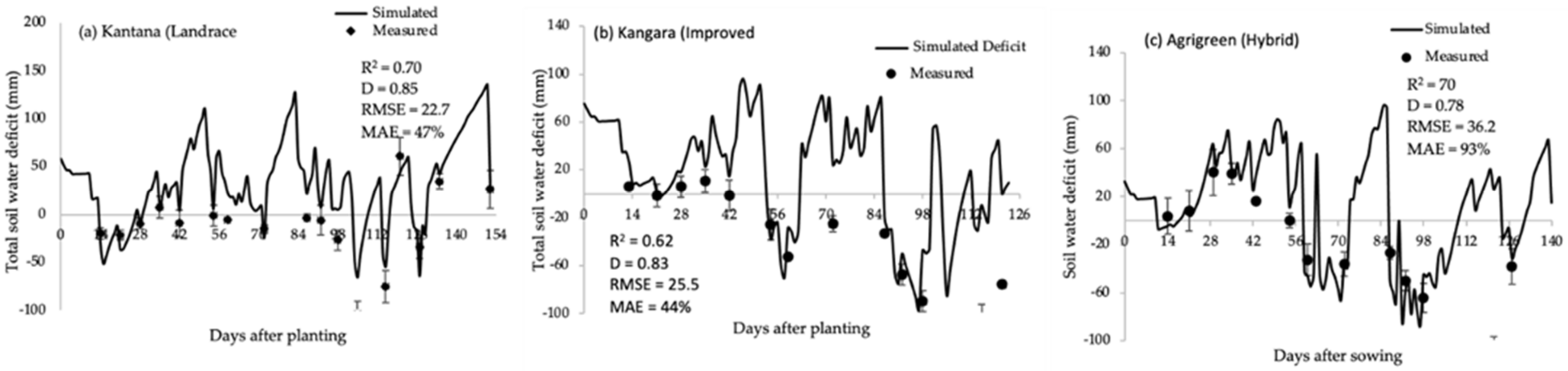
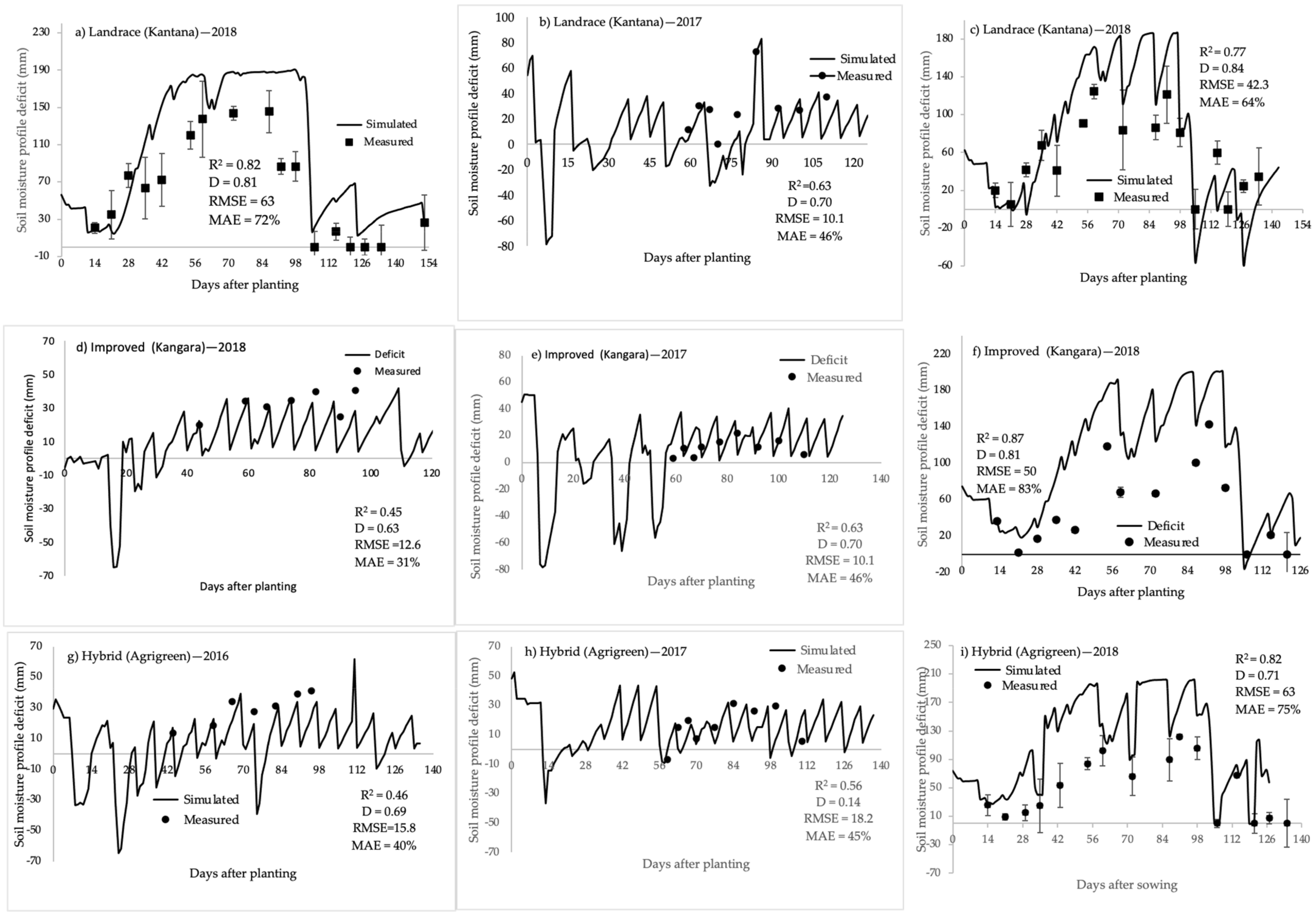
2.1. Soil Water Balance
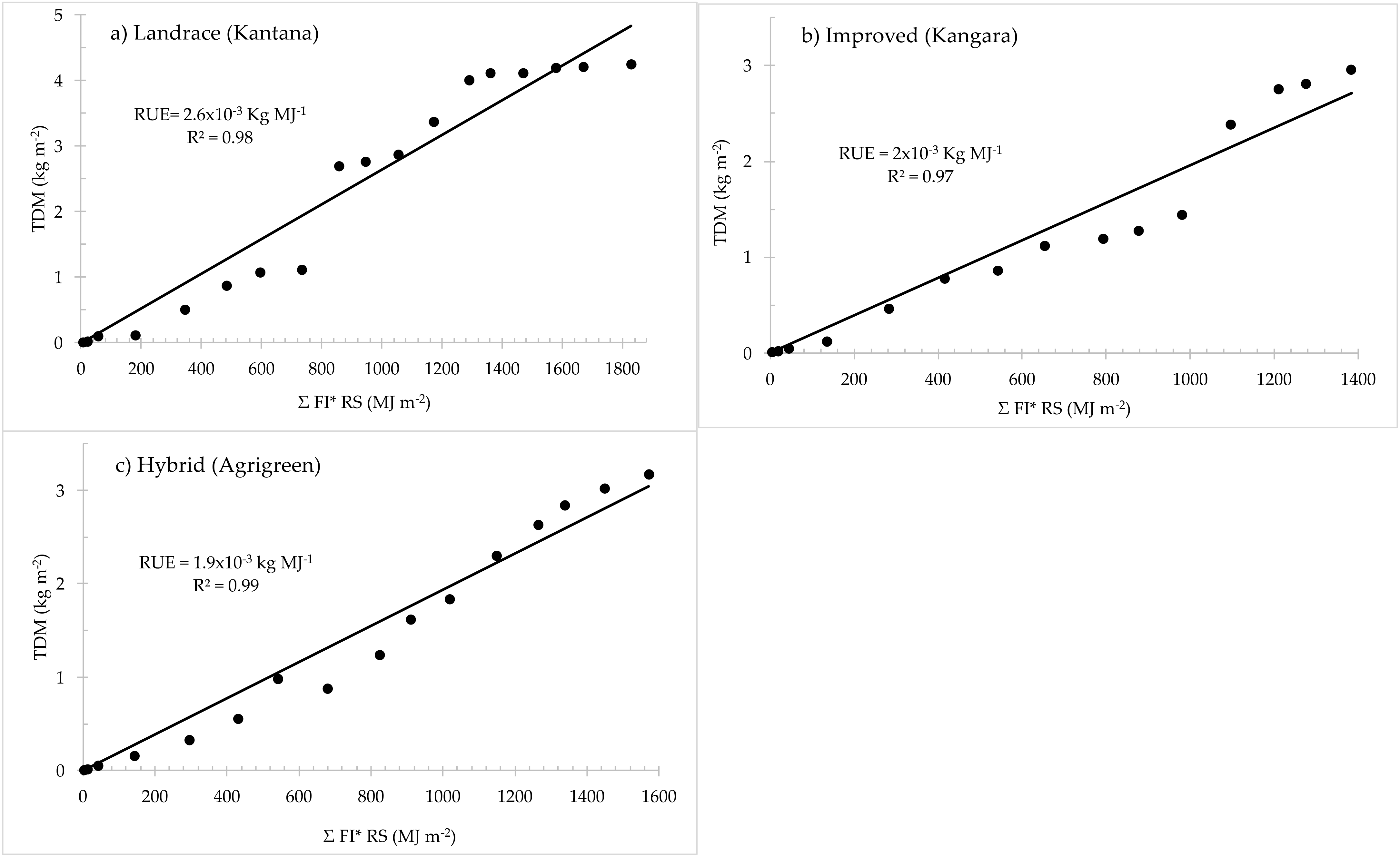
2.1.1. Radiation Limited Dry Matter Production
2.1.2. Water Limited Dry Matter Production

| Crop Parameter | Value | Literature Value | Reference | ||
|---|---|---|---|---|---|
| Hybrid (Agrigreen) | Landrace (Kantana) | Improved (Kangara) | |||
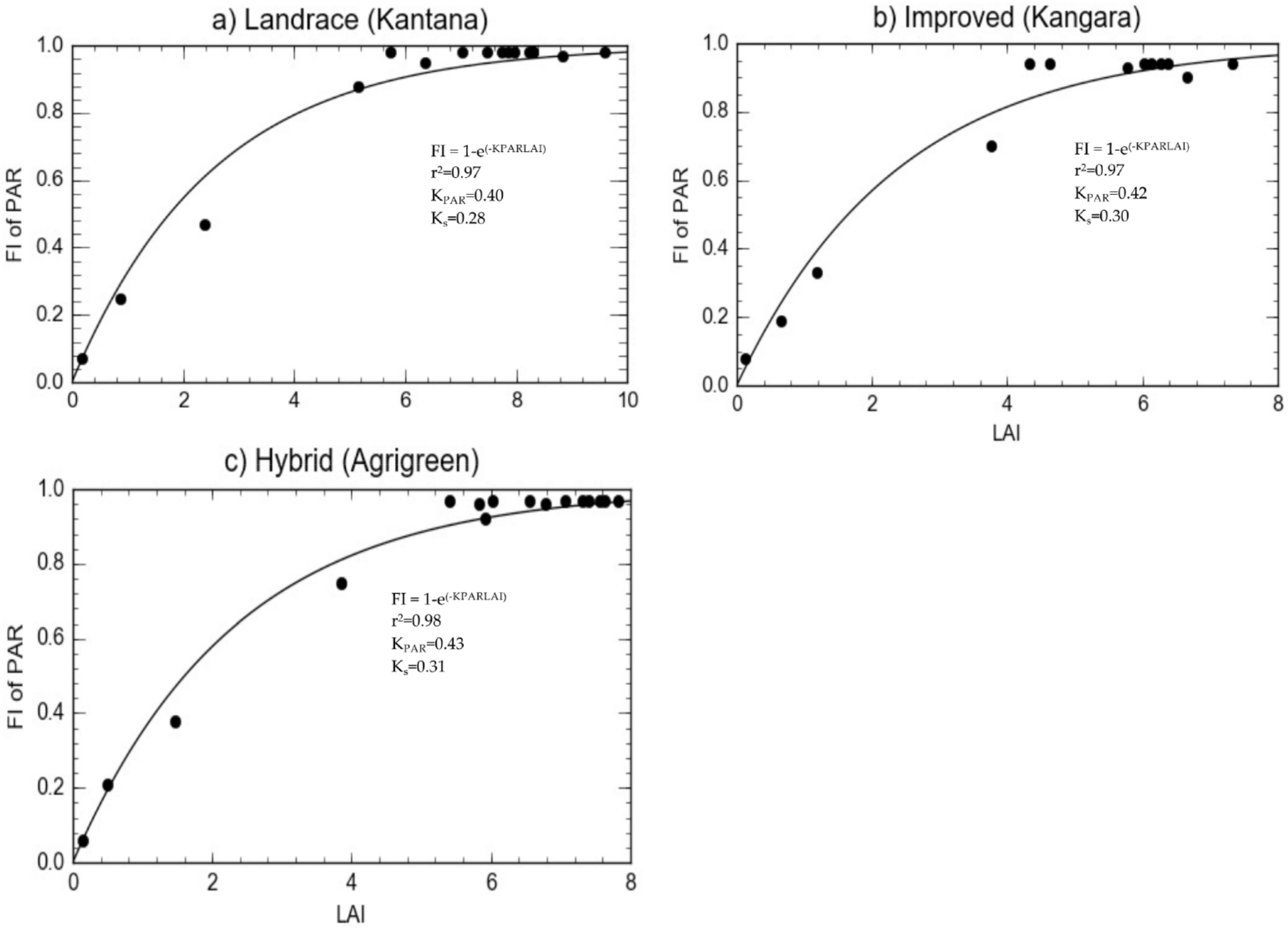
| Canopy extinction coefficient for photosynthetic active radiation KPAR | 0.43 | 0.40 | 0.42 | 0.64–0.42 | [70,71] |
| Canopy extinction coefficient for total solar radiation Ks | 0.31 | 0.28 | 0.30 | 0.49 | [72] |
| Radiation use efficiency, RUE (kg MJ−1) | 0.0019 | 0.0026 | 0.002 | 0.0003–0.00261 | [64,65,73,74,75,76] |
| Dry matter/transpiration ratio corrected for vapour pressure deficit, DWR (Pa) | 11.3 | 15.8 | 11.2 | ||
| Water use efficiencygrain, WUE (kg m−3) | 1.43 | 1.29 | 1.23 | 3.16–10.4 | [11,12] |
| Water use efficiencybiomass, WUE (kg m−3) | 4.83 | 9.16 | 4.69 | 8.56–39.6 | [11,12] |
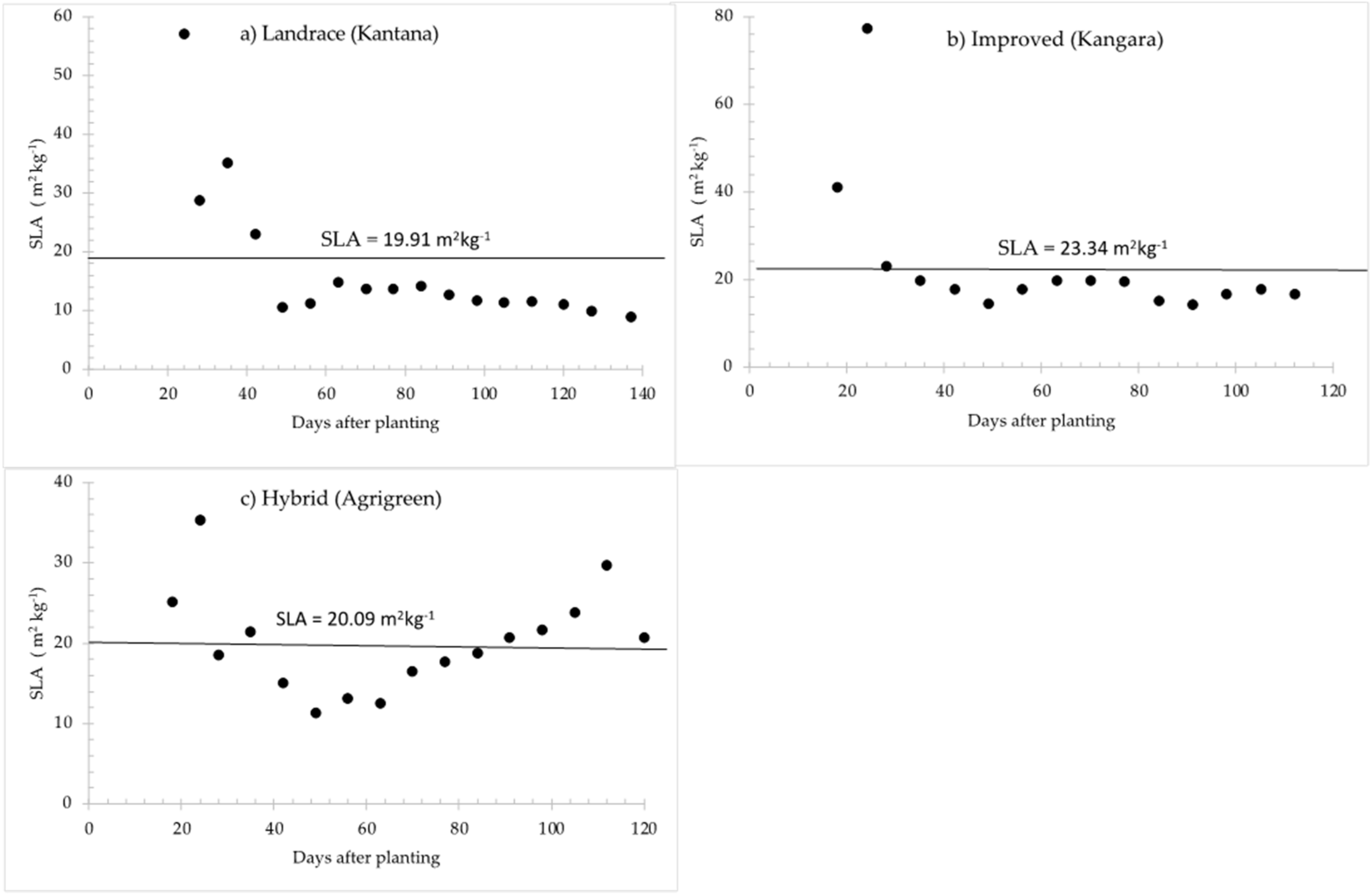
| Specific leaf area, SLA (m2 kg−1) | 22.49 | 19.91 | 23.34 | 11.98–33 | [77,78,79] |
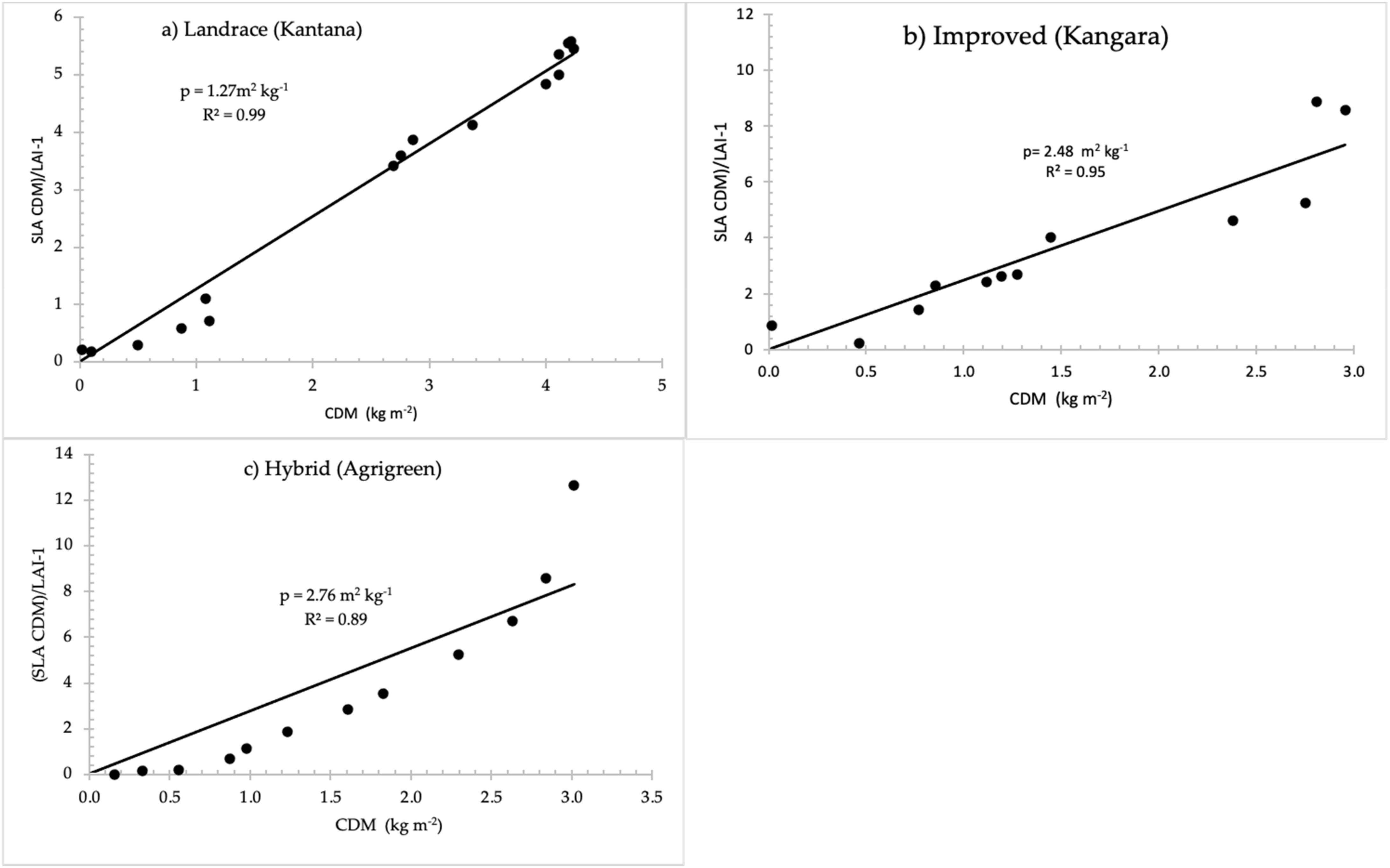
| Leaf-stem partition parameter, PART (m2 kg−1) | 2.76 | 1.27 | 2.48 | ||
| Maximum root depth (m) | 1.00 | 1.00 | 1.00 | 1.8 | [80,81,82] |
| Maximum crop height (m) | 2.87 | 4.22 | 2.80 | 4.9 | [6] |
| Maximum transpiration rate (mm d−1) | 9 * | 9 * | 9 * | 9.2 | [83] |
| Base temperature (°C) | 10 * | 10 * | 10 * | 10–12 | [67,84,85] |
| Optimum temperature (°C) | 33 * | 33 * | 33 * | 33–34 | [67,84] |
| Maximum temperature (°C) | 45 * | 45 * | 45 * | 45–47 | [67,84,85] |
| Emergence day degrees (°C d) | 60 | 64 | 60 | 60 | [67] |
| Flowering day degrees (°C d) | 900 | 1058 | 832 | 954–1265 | [84] |
| Maturity day degrees (°C d) | 1686 | 2124 | 1480 | 1552–1714 | [84] |
| Transition day degrees (°C d) | 670 | 780 | 655 | 415–621 | [84] |
| Total dry matter yield at emergence (kg m−2) | 0.0019 | 0.0019 | 0.0019 | ||
| Stress index | 0.30 * | 0.30 * | 0.30 * | 0.30–0.50 | [86] |
2.1.3. Growing Degree Days
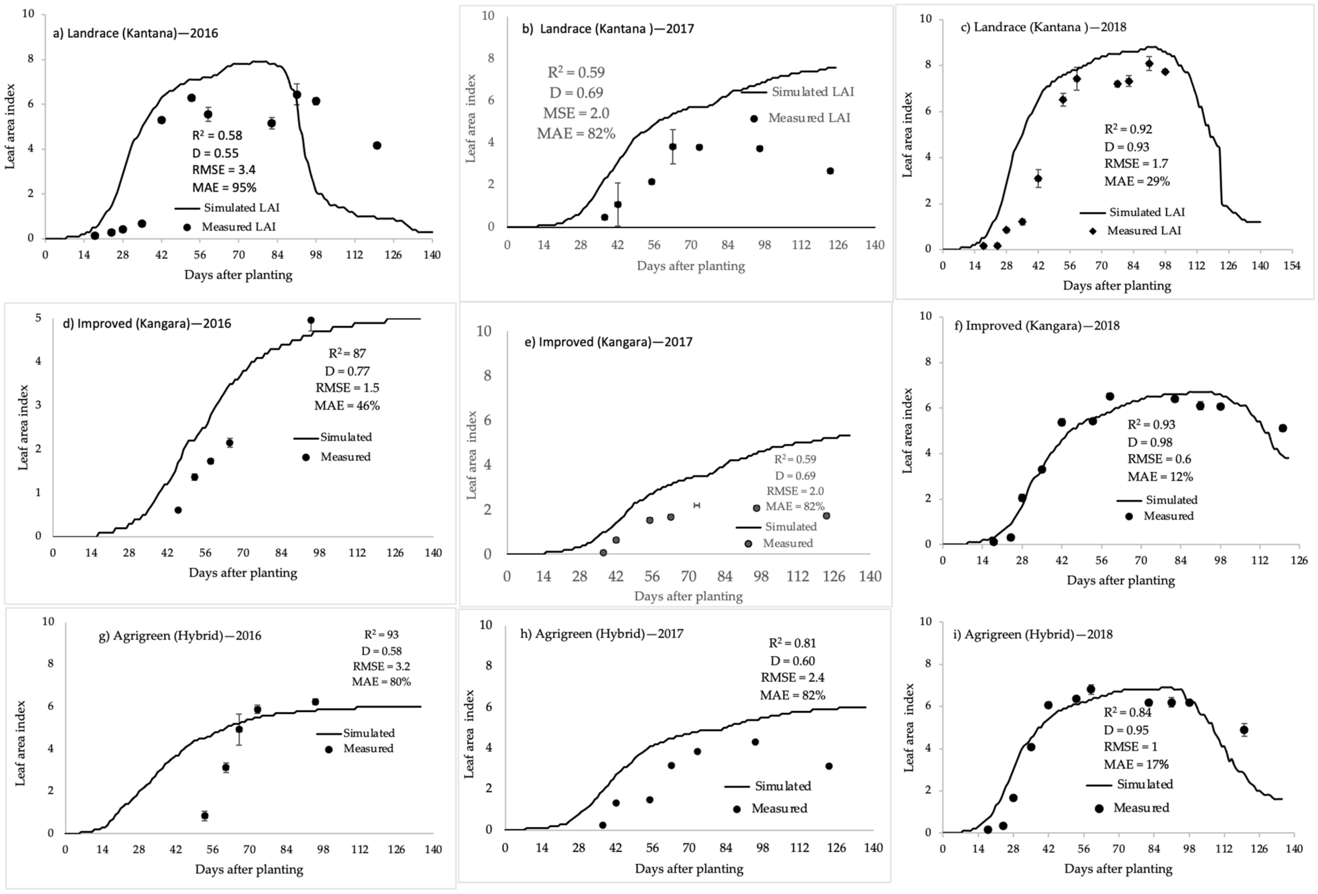
2.1.4. Radiation Interception
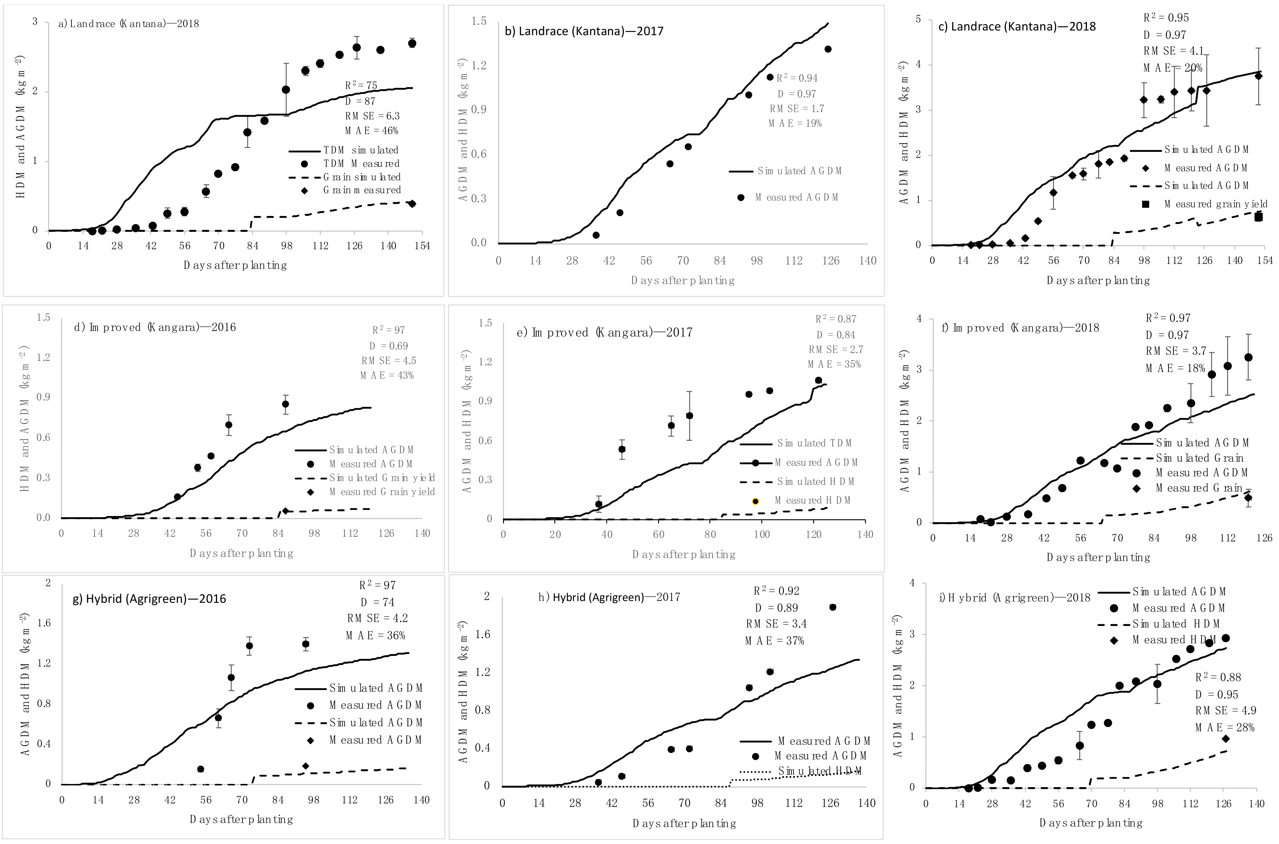
2.1.5. Above-Ground Biomass Partitioning
2.1.6. Specific Leaf Area
2.2. Model Calibration
2.3. Model Validation
3. Discussion
3.1. Soil Water Balance
3.2. Radiation Limited Dry Matter Production
3.3. Light Interception and Biomass Accumulation
3.4. Specific Leaf Area
4. Materials and Methods
4.1. Experiment Description
4.2. Soil Water Balance
4.3. Soil Water Content Estimation
4.4. Model Calibration
4.4.1. VPD and SI Parameters
4.4.2. Radiation Limited Dry Matter Production
4.4.3. Water Limited Dry Matter Production
4.4.4. Growing Degree Days
4.4.5. Radiation Interception
4.4.6. Above-Ground Biomass Partitioning
4.5. Data Collection for Model Calibration
4.6. Model Validation
- 1.
- Irrigated weekly to field capacity until the end of the growing season.
- 2.
- Irrigated to field capacity on a fortnightly basis until the end of the growing season.
- 3.
- Rainfed (dryland) until the end of the growing season.
5. Conclusions
Author Contributions
Funding
Institutional Review Board Statement
Informed Consent Statement
Data Availability Statement
Acknowledgments
Conflicts of Interest
References
- Andrews, D.; Kumar, K. Pearl millet for food, feed, and forage. Adv. Agron. 1992, 48, 89–139. [Google Scholar]
- Bouajila, A.; Lamine, M.; Rahali, F.; Melki, I.; Prakash, G.; Ghorbel, A. Pearl millet populations characterized by Fusarium prevalence, morphological traits, phenolic content, and antioxidant potential. J. Sci. Food Agric. 2020, 100, 4172–4181. [Google Scholar] [CrossRef] [PubMed]
- Varshney, R.K.; Shi, C.; Thudi, M.; Mariac, C.; Wallace, J.; Qi, P.; Zhang, H.; Zhao, Y.; Wang, X.; Rathore, A. Pearl millet genome sequence provides a resource to improve agronomic traits in arid environments. Nat. Biotechnol. 2017, 35, 969–976. [Google Scholar] [CrossRef] [PubMed] [Green Version]
- Brunken, J.; De Wet, J.; Harlan, J. The morphology and domestication of pearl millet. Econ. Bot. 1977, 31, 163–174. [Google Scholar] [CrossRef]
- Chandana, P.; Lata, A.M.; Khan, M.A.; Krishna, A. Influence of Nutrient Management Practices on Growth and Yield of Pearl Millet in Melia dubia Based Agri-Silvi System. Int. J. Curr. Microbiol. App. Sci. 2018, 7, 443–454. [Google Scholar] [CrossRef]
- Upadhyaya, H.; Reddy, K.; Gowda, C. Pearl millet germplasm at ICRISAT genebank-status and impact. J. SAT Agric. Res. 2007, 3, 5. [Google Scholar]
- Baltensperger, D.D. Progress with proso, pearl and other millets. In Trends in New Crops and New Uses; ASHS Press: Alexandria, VA, USA, 2002; pp. 100–103. [Google Scholar]
- Jukanti, A.; Gowda, C.L.; Rai, K.; Manga, V.; Bhatt, R. Crops that feed the world 11. Pearl Millet (Pennisetum glaucum L.): An important source of food security, nutrition and health in the arid and semi-arid tropics. Food Secur. 2016, 8, 307–329. [Google Scholar] [CrossRef]
- Nambiar, V.S.; Dhaduk, J.; Sareen, N.; Shahu, T.; Desai, R. Potential functional implications of pearl millet (Pennisetum glaucum) in health and disease. J. Appl. Pharm. Sci. 2011, 1, 62. [Google Scholar]
- Tako, E.; Reed, S.M.; Budiman, J.; Hart, J.J.; Glahn, R.P. Higher iron pearl millet (Pennisetum glaucum L.) provides more absorbable iron that is limited by increased polyphenolic content. J. Nutr. 2015, 14, 11. [Google Scholar] [CrossRef] [Green Version]
- Ausiku, A.P.; Annandale, J.G.; Steyn, J.M.; Sanewe, A.J. Improving Pearl Millet (Pennisetum glaucum) Productivity through Adaptive Management of Water and Nitrogen. Water 2020, 12, 422. [Google Scholar] [CrossRef] [Green Version]
- Maman, N.; Lyon, D.J.; Mason, S.C.; Galusha, T.D.; Higgins, R. Pearl millet and grain sorghum yield response to water supply in Nebraska. Agron. J. 2003, 95, 1618–1624. [Google Scholar] [CrossRef] [Green Version]
- Gulia, S.; Wilson, J.; Carter, J.; Singh, B. Progress in grain pearl millet research and market development. In Issues in New Crops and New Uses; ASHS Press: Alexandria, VA, USA, 2007; pp. 196–203. [Google Scholar]
- Basnayake, J.; Fukai, S.; Ouk, M. Contribution of potential yield, drought tolerance and escape to adaptation of 15 rice varieties in rainfed lowlands in Cambodia. In Proceedings of the Australian Agronomy Conference, Australian Society of Agronomy, Birsbane, Australia, 10–14 September 2006. [Google Scholar]
- Singels, A.; Annandale, J.G.; Jager, J.D.; Schulze, R.E.; Inman-Bamber, N.; Durand, W.; Rensburg, L.V.; Heerden, P.V.; Crosby, C.T.; Green, G.C. Modelling crop growth and crop water relations in South Africa: Past achievements and lessons for the future. S. Afr. J. Plant Soil 2010, 27, 49–65. [Google Scholar] [CrossRef]
- Bonan, G. Climate Change and Terrestrial Ecosystem Modeling; Cambridge University Press: Cambridge, UK, 2019. [Google Scholar]
- Ciais, P.; Sabine, C.; Bala, G.; Bopp, L.; Brovkin, V.; Canadell, J.; Chhabra, A.; DeFries, R.; Galloway, J.; Heimann, M. Climate Change 2013: The Physical Science Basis. Contribution of Working Group I to the Fifth Assessment Report of the Intergovernmental Panel on Climate Change; Tignor, M., Allen, S.K., Boschung, J., Nauels, A., Xia, Y., Bex, V., Midgley, P.M., Eds.; Cambridge University Press: Cambridge, UK, 2013. [Google Scholar]
- Kasampalis, D.A.; Alexandridis, T.K.; Deva, C.; Challinor, A.; Moshou, D.; Zalidis, G. Contribution of remote sensing on crop models: A review. J. Imaging 2018, 4, 52. [Google Scholar] [CrossRef] [Green Version]
- Rengel, Z. Mechanistic simulation models of nutrient uptake: A review. Plant Soil 1993, 152, 161–173. [Google Scholar] [CrossRef]
- Van Noordwijk, M.; De Willigen, P.; Ehlert, P. A simple model of P uptake by crops as a possible basis for P fertilizer recommendations. Neth. J. Agric. Sci. 1990, 38, 317–332. [Google Scholar] [CrossRef]
- Hoffland, E.; Bloemhof, H.; Leffelaar, P.; Findenegg, G.; Nelemans, J. Simulation of nutrient uptake by a growing root system considering increasing root density and inter-root competition. In Plant Nutrition—Physiology and Applications; Springer: Berlin/Heidelberg, Germany, 1990; pp. 9–15. [Google Scholar]
- Vahrmeijer, J.; Annandale, J.G.; Steyn, J.M.; Bristow, K.L. Model parameters of four important vegetable crops for improved water use and yield estimation. Water SA 2018, 44, 528–538. [Google Scholar] [CrossRef] [Green Version]
- Murthy, V.R.K. Crop growth modeling and its applications in agricultural meteorology. In Satellite Remote Sensing and GIS Applications in Agricultural Meteorology; World Meteorological Organisation: Geneva, Switzerland, 2004; Volume 235. [Google Scholar]
- Diekkrüger, B.; Söndgerath, D.; Kersebaum, K.; McVoy, C. Validity of agroecosystem models a comparison of results of different models applied to the same data set. Ecol. Model. 1995, 81, 3–29. [Google Scholar] [CrossRef]
- Eitzinger, J.; Trnka, M.; Hösch, J.; Žalud, Z.; Dubrovský, M. Comparison of CERES, WOFOST and SWAP models in simulating soil water content during growing season under different soil conditions. Ecol. Model. 2004, 171, 223–246. [Google Scholar] [CrossRef]
- Kersebaum, K.C. Modelling nitrogen dynamics in soil–crop systems with HERMES. In Modelling Water and Nutrient Dynamics in Soil–Crop Systems; Springer: Berlin/Heidelberg, Germany, 2007; pp. 147–160. [Google Scholar]
- Boote, K.J.; Jones, J.W.; Pickering, N.B. Potential uses and limitations of crop models. Agron. J. 1996, 88, 704–716. [Google Scholar] [CrossRef]
- Acutis, M.; Ducco, G.; Grignani, C. Stochastic use of the LEACHN model to forecast nitrate leaching in different maize cropping systems. Eur. J. Agron. 2000, 13, 191–206. [Google Scholar] [CrossRef]
- Donatelli, M.; Acutis, M.; Danuso, F.; Mazzetto, F.; Nasuelli, P.; Nelson, R.; Omicini, A.; Speroni, M.; Trevisan, M.; Tugnoli, V. Integrated procedures for evaluating technical, environmental and economical aspects in farms: The SIPEAA project. Proc. Seventh ESA 2002, 15–18. [Google Scholar]
- Bechini, L.; Bocchi, S.; Maggiore, T. Spatial interpolation of soil physical properties for irrigation planning. A simulation study in northern Italy. Eur. J. Agron. 2003, 19, 1–14. [Google Scholar] [CrossRef]
- Gömann, H.; Kreins, P.; Kunkel, R.; Wendland, F. Model based impact analysis of policy options aiming at reducing diffuse pollution by agriculture—A case study for the river Ems and a sub-catchment of the Rhine. Environ. Model. Softw. 2005, 20, 261–271. [Google Scholar] [CrossRef]
- Lewis, D.; McGechan, M.; McTaggart, I.P. Simulating field-scale nitrogen management scenarios involving fertiliser and slurry applications. Agric. Syst. 2003, 76, 159–180. [Google Scholar] [CrossRef]
- Johnsson, H.; Larsson, M.; Mårtensson, K.; Hoffmann, M. SOILNDB: A decision support tool for assessing nitrogen leaching losses from arable land. Environ. Model. Softw. 2002, 17, 505–517. [Google Scholar] [CrossRef]
- Rossing, W.; Meynard, J.M.; Van Ittersum, M. Model-based explorations to support development of sustainable farming systems: Case studies from France and the Netherlands. Eur. J. Agron. 1997, 7, 271–283. [Google Scholar] [CrossRef]
- Wolf, J.; Beusen, A.; Groenendijk, P.; Kroon, T.; Rötter, R.; Van Zeijts, H. The integrated modeling system STONE for calculating nutrient emissions from agriculture in the Netherlands. Environ. Model. Softw. 2003, 18, 597–617. [Google Scholar] [CrossRef]
- Whisler, F.; Acock, B.; Baker, D.; Fye, R.; Hodges, H.; Lambert, J.; Lemmon, H.; McKinion, J.; Reddy, V. Crop simulation models in agronomic systems. In Advances in Agronomy; Elsevier: Amsterdam, The Netherlands, 1986; Volume 40, pp. 141–208. [Google Scholar]
- Evans, L.T. Crop Evolution, Adaptation and Yield; Cambridge University Press: Cambridge, UK, 1996. [Google Scholar]
- De Vries, F.P.; Rabbinge, R.; Groot, J. Potential and attainable food production and food security in different regions. Philos. Trans. R. Soc. B Biol. Sci. 1997, 352, 917–928. [Google Scholar] [CrossRef] [Green Version]
- Wang, E.; Robertson, M.; Hammer, G.; Carberry, P.S.; Holzworth, D.; Meinke, H.; Chapman, S.; Hargreaves, J.; Huth, N.; McLean, G. Development of a generic crop model template in the cropping system model APSIM. Eur. J. Agron. 2002, 18, 121–140. [Google Scholar] [CrossRef]
- Keating, B.A.; Carberry, P.S.; Hammer, G.L.; Probert, M.E.; Robertson, M.J.; Holzworth, D.; Huth, N.I.; Hargreaves, J.N.; Meinke, H.; Hochman, Z. An overview of APSIM, a model designed for farming systems simulation. Eur. J. Agron. 2003, 18, 267–288. [Google Scholar] [CrossRef] [Green Version]
- Aggarwal, P.K.; Kalra, N.; Chander, S.; Pathak, H. InfoCrop: A dynamic simulation model for the assessment of crop yields, losses due to pests, and environmental impact of agro-ecosystems in tropical environments. I. Model description. Agric. Syst. 2006, 89, 1–25. [Google Scholar] [CrossRef]
- Ewert, F.; Rötter, R.P.; Bindi, M.; Webber, H.; Trnka, M.; Kersebaum, K.C.; Olesen, J.E.; van Ittersum, M.K.; Janssen, S.; Rivington, M. Crop modelling for integrated assessment of risk to food production from climate change. Environ. Model. Softw. 2015, 72, 287–303. [Google Scholar] [CrossRef]
- Asseng, S.; Ewert, F.; Martre, P.; Rötter, R.P.; Lobell, D.B.; Cammarano, D.; Kimball, B.A.; Ottman, M.J.; Wall, G.; White, J.W. Rising temperatures reduce global wheat production. Nat. Clim. Change 2015, 5, 143. [Google Scholar] [CrossRef]
- Phalan, B.; Green, R.; Balmford, A. Closing yield gaps: Perils and possibilities for biodiversity conservation. Philos. Trans. R. Soc. B Biol. Sci. 2014, 369, 20120285. [Google Scholar] [CrossRef] [Green Version]
- Mueller, N.D.; Gerber, J.S.; Johnston, M.; Ray, D.K.; Ramankutty, N.; Foley, J.A. Closing yield gaps through nutrient and water management. Nature 2012, 490, 254–257. [Google Scholar] [CrossRef]
- Jovanovic, N.; Annandale, J.; Mhlauli, N. Field water balance and SWB parameter determination of six winter vegetable species. Water SA 1999, 25, 191–196. [Google Scholar]
- Beletse, Y.; Annandale, J.; Steyn, J.; Hall, I.; Aken, M. Can crops be irrigated with sodium bicarbonate rich CBM deep aquifer water? Theoretical and field evaluation. Ecol. Eng. 2008, 33, 26–36. [Google Scholar] [CrossRef]
- Asseng, S.; Ewert, F.; Rosenzweig, C.; Jones, J.W.; Hatfield, J.L.; Ruane, A.C.; Boote, K.J.; Thorburn, P.J.; Rötter, R.P.; Cammarano, D. Uncertainty in simulating wheat yields under climate change. Nat. Clim. Change 2013, 3, 827–832. [Google Scholar] [CrossRef] [Green Version]
- Annandale, J.; Jovanovic, N.; Benade, N.; Tanner, P. Modelling the long-term effect of irrigation with gypsiferous water on soil and water resources. Agric. Ecosyst. Environ. 1999, 76, 109–119. [Google Scholar] [CrossRef]
- Jovanovic, N.; Annandale, J.; Nel, A. Calibration and validation of the SWB model for sunflower (Helianthus annuus L.). S. Afr. J. Plant Soil 2000, 17, 117–123. [Google Scholar] [CrossRef]
- Du Sautoy, N.; Jovanovic, N.; Annandale, J. Water balance simulation of a peach orchard using the SWB model. S. Afr. J. Plant Soil 2003, 20, 169–175. [Google Scholar] [CrossRef] [Green Version]
- Annandale, J.; Jovanovic, N.; Campbell, G.; Du Sautoy, N.; Lobit, P. Two-dimensional solar radiation interception model for hedgerow fruit trees. Agric. For. Meteorol. 2004, 121, 207–225. [Google Scholar] [CrossRef]
- Fessehazion, M.K.; Annandale, J.G.; Everson, C.S.; Stirzaker, R.J.; Tesfamariam, E.H. Evaluating of soil water balance (SWB-Sci) model for water and nitrogen interactions in pasture: Example using annual ryegrass. Agric. Water Manag. 2014, 146, 238–248. [Google Scholar] [CrossRef]
- Tesfamariam, E.H.; Annandale, J.G.; Steyn, J.M.; Stirzaker, R.J.; Mbakwe, I. Use of the SWB-Sci model for nitrogen management in sludge-amended land. Agric. Water Manag. 2015, 152, 262–276. [Google Scholar] [CrossRef] [Green Version]
- Pereira, L.S.; Allen, R.G.; Smith, M.; Raes, D. Crop evapotranspiration estimation with FAO56: Past and future. Agric. Water Manag. 2015, 147, 4–20. [Google Scholar] [CrossRef]
- Goudriaan, J.; Van Laar, H. Modelling Potential Crop Growth Processes: Textbook with Exercises; Springer Science & Business Media: Berlin/Heidelberg, Germany, 2012; Volume 2. [Google Scholar]
- Bechini, L.; Bocchi, S.; Maggiore, T.; Confalonieri, R. Parameterization of a crop growth and development simulation model at sub-model components level. An example for winter wheat (Triticum aestivum L.). Environ. Model. Softw. 2006, 21, 1042–1054. [Google Scholar] [CrossRef]
- Fessehazion, M.K.; Stirzaker, R.J.; Annandale, J.G.; Everson, C.S. Improving nitrogen and irrigation water use efficiency through adaptive management: A case study using annual ryegrass. Agric. Ecosyst. Environ. 2011, 141, 350–358. [Google Scholar] [CrossRef] [Green Version]
- Donatelli, M.; Stöckle, C.; Ceotto, E.; Rinaldi, M. Evaluation of CropSyst for cropping systems at two locations of northern and southern Italy. Eur. J. Agron. 1997, 6, 35–45. [Google Scholar] [CrossRef]
- Giardini, L.; Berti, A.; Morari, F. Simulation of two cropping systems with EPIC and CropSyst models. Ital. J. Agron. 1998, 2, 29–38. [Google Scholar]
- Bellocchi, G.; Silvestri, N.; Mazzoncini, M.; Meini, S. Using the CropSyst Model in Continuous Rainfed Maize (Zea mais L.) under Alternative Management Options. Ital. J. Agron. 2002, 6, 43–56. [Google Scholar]
- Sun, H.; Shen, Y.; Yu, Q.; Flerchinger, G.N.; Zhang, Y.; Liu, C.; Zhang, X. Effect of precipitation change on water balance and WUE of the winter wheat–summer maize rotation in the North China Plain. Agric. Water Manag. 2010, 97, 1139–1145. [Google Scholar] [CrossRef]
- Squire, G.; Gregory, P.; Monteith, J.; Russell, M.; Singh, P. Control of water use by pearl millet (Pennisetum typhoides). Exp. Agric. 1984, 20, 135–149. [Google Scholar] [CrossRef] [Green Version]
- Reddy, M.; Willey, R. Growth and resource use studies in an intercrop of pearl millet/groundnut. Field Crop. Res. 1981, 4, 13–24. [Google Scholar] [CrossRef] [Green Version]
- Squire, G.; Marshall, B.; Terry, A.; Monteith, J. Response to temperature in a stand of pearl millet: VI. Light interception and dry matter production. J. Exp. Bot. 1984, 35, 599–610. [Google Scholar] [CrossRef]
- Craufurd, P.; Bidinger, F. Effect of the duration of the vegetative phase on crop growth, development and yield in two contrasting pearl millet hybrids. J. Agric. Sci. 1988, 110, 71–79. [Google Scholar] [CrossRef] [Green Version]
- Ong, C.; Monteith, J. Response of pearl millet to light and temperature. Field Crop. Res. 1985, 11, 141–160. [Google Scholar] [CrossRef] [Green Version]
- Ram, N.; Sheoran, K.; Sastry, C.S. Radiation efficiency and its efficiency in dry biomass production of pearl millet cultivars. Ann. Agric. Res. 1999, 20, 286–291. [Google Scholar]
- Payne, W.A. Managing yield and water use of pearl millet in the Sahel. Agron. J. 1997, 89, 481–490. [Google Scholar] [CrossRef] [Green Version]
- Jarwal, S.; Singh, P.; Virmani, S. Influence of planting geometry on photosynthetically active radiation interception and dry matter production relationships in pearl millet. Biomass 1990, 21, 273–284. [Google Scholar] [CrossRef] [Green Version]
- Jovanovic, N.; Annandale, J. Measurement of radiant interception of crop canopies with the LAI-2000 plant canopy analyzer. S. Afr. J. Plant Soil 1998, 15, 6–13. [Google Scholar] [CrossRef] [Green Version]
- Annandale, J.; Campbell, G.; Olivier, F.; Jovanovic, N. Predicting crop water uptake under full and deficit irrigation: An example using pea (Pisum sativum L. cv. Puget). Irrig. Sci. 2000, 19, 65–72. [Google Scholar] [CrossRef]
- Azam-Ali, S.; Gregory, P.; Monteith, J. Effects of planting density on water use and productivity of pearl millet (Pennisetum typhoides) grown on stored water. II. Water use, light interception and dry matter production. Exp. Agric. 1984, 20, 215–224. [Google Scholar] [CrossRef] [Green Version]
- Squire, G.R. The Physiology of Tropical Crop Production; CAB International: Wallingford, UK, 1990. [Google Scholar]
- Begue, A.; Desprat, J.; Imbernon, J.; Baret, F. Radiation use efficiency of pearl millet in the Sahelian zone. Agric. For. Meteorol. 1991, 56, 93–110. [Google Scholar] [CrossRef]
- Craufurd, P.; Bidinger, F. Potential and realized yield in pearl millet (Pennisetum americanum) as influenced by plant population density and life-cycle duration. Field Crop. Res. 1989, 22, 211–225. [Google Scholar] [CrossRef] [Green Version]
- Singh, A.; Goyal, V.; Mishra, A.; Parihar, S. Performance evaluation of Crop Syst simulation model for pearlmillet (Pennisetum glaucum)-chickpea (Cicer arietinum) cropping system. Indian J. Agron. 2015, 60, 516–523. [Google Scholar]
- Van Heemst, H. Plant Data Values Required for Simple Crop Growth Simulation Models: Review and Bibliography; Centre for Agrobiological Research and Agricultural University: Wageningen, The Netherlands, 1988. [Google Scholar]
- Monteith, J.; Huda, A.; Midya, D. Modeling Sorghum and Pearl Millet. Modeling the Growth and Development of Sorghum and Pearl Millet; International Crops Research Institute for the Semi-Arid Tropics: Andhra Pradesh, India, 1989. [Google Scholar]
- Wet, J.; Bidinger, F.; Peacock, J. Pearl Millet (Pennisetum glaucum)—A Cereal of the Sahel; Academic Press: Cambridge, MA, USA, 1992. [Google Scholar]
- Klaij, M.; Vachaud, G. Seasonal water balance of a sandy soil in Niger cropped with pearl millet, based on profile moisture measurements. Agric. Water Manag. 1992, 21, 313–330. [Google Scholar] [CrossRef] [Green Version]
- Gregory, P.; Reddy, M. Root growth in an intercrop of pearl millet/groundnut. Field Crop. Res. 1982, 5, 241–252. [Google Scholar] [CrossRef] [Green Version]
- McIntyre, B.; Riha, S.; Flower, D. Water uptake by pearl millet in a semiarid environment. Field Crop. Res. 1995, 43, 67–76. [Google Scholar] [CrossRef] [Green Version]
- Singh, R.; Joshi, N.; Singh, H. Pearl millet phenology and growth in relation to thermal time under arid environment. J. Agron. Crop Sci. 1998, 180, 83–91. [Google Scholar] [CrossRef]
- Garcia-Huidobro, J.; Monteith, J.; Squire, G. Time, temperature and germination of pearl millet (Pennisetum typhoides S. & H.) I. Constant temperature. J. Exp. Bot. 1982, 33, 288–296. [Google Scholar]
- Teowolde, H.; Voigt, R.L.; Osman, M.; Dobrenz, A.K. Water Stress Indices for Research and Irrigation Scheduling in Pearl Millet; College of Agriculture, University of Arizona: Tucson, AZ, USA, 1987. [Google Scholar]
- Spitters, C. Crop growth models: Their usefulness and limitations. In Proceedings of the VI Symposium on the Timing of Field Production of Vegetables 267, Wageningen, The Netherlands, 21–25 August 1989; pp. 349–368. [Google Scholar]
- Yulin, L.; Johnson, D.A.; Yongzhong, S.; Jianyuan, C.; Zhang, T. Specific leaf area and leaf dry matter content of plants growing in sand dunes. Bot. Bull. Acad. Sin. 2005, 46, 127–134. [Google Scholar]
- Silungwe, F.R.; Graef, F.; Bellingrath-Kimura, S.D.; Tumbo, S.D.; Kahimba, F.C.; Lana, M.A. The management strategies of pearl millet farmers to cope with seasonal rainfall variability in a semi-arid agroclimate. Agronomy 2019, 9, 400. [Google Scholar] [CrossRef] [Green Version]
- Agrawal, S.; Jain, A. Sustainable deployment of solar irrigation pumps: Key determinants and strategies. Wiley Interdiscip. Rev. Energy Environ. 2019, 8, e325. [Google Scholar] [CrossRef]
- Sinclair, T.R.; Muchow, R.C. Radiation use efficiency. In Advances in Agronomy; Elsevier: Amsterdam, The Netherlands, 1999; Volume 65, pp. 215–265. [Google Scholar]
- Monteith, J.L. Validity of the correlation between intercepted radiation and biomass. Agric. For. Meteorol. 1994, 68, 213–220. [Google Scholar] [CrossRef]
- Carretero, R.; Serrago, R.A.; Bancal, M.O.; Perelló, A.E.; Miralles, D.J. Absorbed radiation and radiation use efficiency as affected by foliar diseases in relation to their vertical position into the canopy in wheat. Field Crop. Res. 2010, 116, 184–195. [Google Scholar] [CrossRef]
- Koester, R.P.; Skoneczka, J.A.; Cary, T.R.; Diers, B.W.; Ainsworth, E.A. Historical gains in soybean (Glycine max Merr.) seed yield are driven by linear increases in light interception, energy conversion, and partitioning efficiencies. J. Exp. Bot. 2014, 65, 3311–3321. [Google Scholar] [CrossRef]
- Teixeira, E.I.; George, M.; Herreman, T.; Brown, H.; Fletcher, A.; Chakwizira, E.; de Ruiter, J.; Maley, S.; Noble, A. The impact of water and nitrogen limitation on maize biomass and resource-use efficiencies for radiation, water and nitrogen. Field Crop. Res. 2014, 168, 109–118. [Google Scholar] [CrossRef]
- Arkebauer, T.; Weiss, A.; Sinclair, T.; Blum, A. In defense of radiation use efficiency: A response to Demetriades-Shah et al. (1992). Agric. For. Meteorol. 1994, 68, 221–227. [Google Scholar] [CrossRef]
- Green, C. Genotypic differences in the growth of Triticum aestivum in relation to absorbed solar radiation. Field Crop. Res. 1989, 19, 285–295. [Google Scholar] [CrossRef]
- Robertson, M.; Silim, S.; Chauhan, Y.; Ranganathan, R. Predicting growth and development of pigeonpea: Biomass accumulation and partitioning. Field Crop. Res. 2001, 70, 89–100. [Google Scholar] [CrossRef] [Green Version]
- Ullah, A.; Ahmad, A.; Khaliq, T.; Akhtar, J. Recognizing production options for pearl millet in Pakistan under changing climate scenarios. J. Integr. Agric. 2017, 16, 762–773. [Google Scholar] [CrossRef] [Green Version]
- McIntyre, B.; Flower, D.; Riha, S. Temperature and soil water status effects on radiation use and growth of pearl millet in a semi-arid environment. Agric. For. Meteorol. 1993, 66, 211–227. [Google Scholar] [CrossRef]
- Verdoodt, A.; Van Ranst, E.; Ye, L. Daily simulation of potential dry matter production of annual field crops in tropical environments. Agron. J. 2004, 96, 1739–1753. [Google Scholar] [CrossRef] [Green Version]
- Liu, J.; Fan, Y.; Ma, Y.; Li, Q. Response of photosynthetic active radiation interception, dry matter accumulation, and grain yield to tillage in two winter wheat genotypes. Arch. Agron. Soil Sci. 2020, 66, 1103–1114. [Google Scholar] [CrossRef]
- Jonckheere, I.; Fleck, S.; Nackaerts, K.; Muys, B.; Coppin, P.; Weiss, M.; Baret, F. Methods for leaf area index determination. Part I: Theories, techniques and instruments. Agric. For. Meteorol. 2004, 121, 19–35. [Google Scholar] [CrossRef]
- Huang, S.; Gao, Y.; Li, Y.; Xu, L.; Tao, H.; Wang, P. Influence of plant architecture on maize physiology and yield in the Heilonggang River valley. Crop J. 2017, 5, 52–62. [Google Scholar] [CrossRef] [Green Version]
- Timlin, D.; Kim, S.-H.; Fleisher, D.; Wang, Z.; Reddy, V.R. Maize water use and yield in the solar corridor system: A simulation study. In The Solar Corridor Crop System; Elsevier: Amsterdam, The Netherlands, 2019; pp. 57–78. [Google Scholar]
- Rinaldi, M. Variation of specific leaf area for sugar beet depending on sowing date and irrigation. Ital. J. Agron. 2003, 7, 23–32. [Google Scholar]
- Danalatos, N.; Mitsios, I.; Archontoulis, S. Growth and Biomass Productivity of Kenaf as Biomass Crop in Central Greece. Available online: http://www.cres.gr/biokenaf/files/fs_inferior01_h_files/pdf/articles/Kenaf,%20Danalatos%20et%20al.,%202005.pdf (accessed on 15 January 2022).
- Amanullah, M.J.H.; Nawab, K.; Ali, A. Response of specific leaf area (SLA), leaf area index (LAI) and leaf area ratio (LAR) of maize (Zea mays L.) to plant density, rate and timing of nitrogen application. World Appl. Sci. J. 2007, 2, 235–243. [Google Scholar]
- Wadas, W.; Kosterna, E. Effect of perforated foil and polypropylene fibre covers on assimilation leaf area of early potato cultivars. Plant Soil Environ. 2007, 53, 299. [Google Scholar] [CrossRef] [Green Version]
- Milla, R.; Reich, P.B.; Niinemets, Ü.; Castro-Díez, P. Environmental and developmental controls on specific leaf area are little modified by leaf allometry. Funct. Ecol. 2008, 22, 565–576. [Google Scholar] [CrossRef]
- Reich, P.B.; Walters, M.B.; Ellsworth, D.S. From tropics to tundra: Global convergence in plant functioning. Proc. Natl. Acad. Sci. USA 1997, 94, 13730–13734. [Google Scholar] [CrossRef] [PubMed] [Green Version]
- Field, C.B. On the role of photosynthetic responses in constraining the habitat distribution of rainforest plants. Functl. Plant Biol. 1988, 15, 343–358. [Google Scholar]
- Chapin III, F.S.; Autumn, K.; Pugnaire, F. Evolution of suites of traits in response to environmental stress. Am. Nat. 1993, 142, S78–S92. [Google Scholar] [CrossRef]
- Mooney, H.; Dunn, E. Photosynthetic systems of Mediterranean-climate shrubs and trees of California and Chile. Am. Nat. 1970, 104, 447–453. [Google Scholar] [CrossRef]
- Szulc, P.; Piechota, T.; Jagła, M.; Kowalski, M. A comparative analysis of growth in maize (Zea mays L.) hybrids of different genetic profiles depending on type of nitrogen fertilizer and magnesium dose. Commun. Biometry Crop Sci. 2015, 10, 73–81. [Google Scholar]
- Castro-Díez, P.; Puyravaud, J.-P.; Cornelissen, J. Leaf structure and anatomy as related to leaf mass per area variation in seedlings of a wide range of woody plant species and types. Oecologia 2000, 124, 476–486. [Google Scholar] [CrossRef] [PubMed]
- Federer, C.A. Measuring Forest Evapotranspiration: Theory and Problems; Northeastern Forest Experiment Station, Forest Service, U.S. Department of Agriculture: Washington, DC, USA, 1970. [Google Scholar]
- Ward, R. Measuring evapotranspiration; a review. J. Hydrol. 1971, 13, 1–21. [Google Scholar] [CrossRef]
- Allen, R.G.; Pereira, L.S.; Raes, D.; Smith, M. Crop evapotranspiration-Guidelines for computing crop water requirements-FAO Irrigation and drainage paper 56. Fao Rome 1998, 300, D05109. [Google Scholar]
- Hillel, D. Environmental Soil Physics: Fundamentals, Applications, and Environmental Considerations; Elsevier: Amsterdam, The Netherlands, 1998. [Google Scholar]
- Jackson, R.D.; Idso, S.; Reginato, R.; Pinter, P., Jr. Canopy temperature as a crop water stress indicator. Water Resour. Res. 1981, 17, 1133–1138. [Google Scholar] [CrossRef]
- Jackson, R.D.; Kustas, W.P.; Choudhury, B.J. A reexamination of the crop water stress index. Irrig. Sci. 1988, 9, 309–317. [Google Scholar] [CrossRef]
- Kacira, M.; Ling, P.P.; Short, T.H. Establishing Crop Water Stress Index (CWSI) threshold values for early, non-contact detection of plant water stress. Trans. ASAE 2002, 45, 775. [Google Scholar] [CrossRef]
- Uçak, A.B. Identification of Water Usage Efficiency for Corn (Zea mays L.) Lines Irrigated with Drip Irrigation under Green House Conditions as Per Plant Water Stress Index Evaluations. Turk. Tarımsal Arastırmalar Derg. Turk. J. Agric. Res. 2017, 4, 1–9. [Google Scholar] [CrossRef] [Green Version]
- Monteith, J.L. Climate and the efficiency of crop production in Britain. Philos. Trans. R. Soc. B Biol. Sci. 1977, 281, 277–294. [Google Scholar]
- Campbell, G.S.; Norman, J.M. The light environment of plant canopies. In An Introduction to Environmental Biophysics; Springer: Berlin/Heidelberg, Germany, 1998; pp. 247–278. [Google Scholar]
- Tanner, C.; Sinclair, T. Efficient water use in crop production: Research or research? In Limitations to Efficient Water Use in Crop Production; Wiley: Hoboken, NJ, USA, 1983; pp. 1–27. [Google Scholar]
- Campbell, G.; Van Evert, F. Light interception by plant canopies: Efficiency and architecture. In Resource Capture by Crops; Nottingham University Press: Nottingham, UK, 1994; pp. 35–52. [Google Scholar]
- Ritchie, J.T. Model for predicting evaporation from a row crop with incomplete cover. Water Resour. Res. 1972, 8, 1204–1213. [Google Scholar] [CrossRef] [Green Version]
- Goudriaan, J. Crop Micrometeorology: A Simulation Study; Wageningen University and Research: Wageningen, The Netherlands, 1977. [Google Scholar]
- Yadav, O.; Bidinger, F. Dual-purpose landraces of pearl millet (Pennisetum glaucum) as sources of high stover and grain yield for arid zone environments. Plant Genet. Resourc. 2008, 6, 73. [Google Scholar] [CrossRef]


| Landrace Pearl Millet (Kantana) | Improved Pearl Millet (Kangara) | Hybrid (Agrigreen) | ||||||||||||||||||||
|---|---|---|---|---|---|---|---|---|---|---|---|---|---|---|---|---|---|---|---|---|---|---|
| Date | P | I | ET | D | R | Qi | Qo | ∆S | I | ET | D | R | Qi | Qo | ΔS | I | ET | D | R | Qi | Qo | ΔS |
| 14 December 2017 | 26 | 0 | 13 | 0 | 0 | 315 | 328 | −14 | 0 | 14 | 0 | 0 | 264 | 276 | −13 | 0 | 12 | 0 | 0 | 292 | 306 | −14 |
| 22 December 2017 | 28 | 0 | 7 | 0 | 0 | 328 | 350 | −21 | 28 | 8 | 0 | 0 | 276 | 324 | −48 | 0 | 7 | 0 | 0 | 306 | 327 | −21 |
| 29 December 2017 | 15 | 0 | 13 | 0 | 0 | 350 | 352 | −2 | 4 | 12 | 0 | 0 | 324 | 332 | −8 | 0 | 18 | 1 | 0 | 327 | 322 | 4 |
| 5 January 2018 | 7 | 10 | 29 | 0 | 0 | 352 | 340 | 12 | 8 | 23 | 0 | 0 | 332 | 324 | 8 | 0 | 38 | 1 | 0 | 322 | 290 | 32 |
| 12 January 2018 | 11 | 23 | 50 | 0 | 0 | 340 | 323 | 17 | 31 | 47 | 0 | 0 | 324 | 319 | 5 | 40 | 50 | 0 | 0 | 290 | 291 | −1 |
| 19 January 2018 | 26 | 46 | 55 | 0 | 0 | 323 | 339 | −17 | 40 | 54 | 0 | 0 | 319 | 332 | −12 | 51 | 54 | 0 | 0 | 291 | 314 | −23 |
| 31 January 2018 | 34 | 39 | 81 | 0 | 0 | 339 | 331 | 8 | 72 | 81 | 0 | 0 | 332 | 356 | −25 | 71 | 81 | 8 | 0 | 314 | 330 | −16 |
| 5 February 2018 | 12 | 37 | 45 | 0 | 0 | 331 | 336 | −4 | 50 | 36 | 0 | 0 | 356 | 383 | −27 | 60 | 36 | 4 | 0 | 330 | 363 | −32 |
| 18 February 2018 | 79 | 46 | 87 | 28 | 0 | 336 | 345 | −10 | 0 | 87 | 19 | 0 | 383 | 355 | 27 | 42 | 89 | 28 | 0 | 363 | 366 | −3 |
| 5 March 2018 | 15 | 60 | 81 | 6 | 0 | 345 | 334 | 12 | 81 | 81 | 7 | 0 | 355 | 363 | −8 | 66 | 84 | 6 | 0 | 366 | 357 | 9 |
| 10 March 2018 | 3 | 31 | 31 | 1 | 0 | 334 | 336 | −2 | 63 | 31 | 0 | 0 | 363 | 398 | −34 | 52 | 31 | 1 | 0 | 357 | 380 | −23 |
| 16 March 2018 | 2 | 59 | 40 | 1 | 0 | 336 | 357 | −21 | 60 | 40 | 1 | 0 | 398 | 420 | −22 | 52 | 39 | 1 | 0 | 380 | 395 | −14 |
| 24 March 2018 | 209 | 0 | 44 | 88 | 0 | 357 | 434 | −77 | 0 | 44 | 64 | 0 | 420 | 521 | −101 | 0 | 45 | 51 | 0 | 395 | 508 | −113 |
| 2 April 2018 | 8 | 38 | 40 | 34 | 0 | 434 | 406 | 29 | 0 | 41 | 53 | 0 | 521 | 435 | 86 | 24 | 41 | 29 | 0 | 508 | 470 | 38 |
| 8 April 2018 | 1 | 16 | 28 | 3 | 0 | 406 | 391 | 14 | 0 | 28 | 3 | 0 | 470 | 440 | 30 | |||||||
| 14 April 2018 | 64 | 0 | 25 | 17 | 0 | 391 | 413 | −22 | ||||||||||||||
| Landrace Pearl Millet (Kantana) | Improved Pearl Millet (Kantana) | Hybrid (Agrigreen) | ||||||||||||||||
|---|---|---|---|---|---|---|---|---|---|---|---|---|---|---|---|---|---|---|
| P | I | ET | D | R | ETo | AvgVPD | I | ET | D | R | ETo | AvgVPD | I | ET | D | R | ETo | AvgVPD |
| 542 | 405 | 670 | 179 | 0 | 436 | 0.78 | 437 | 598 | 144 | 0 | 412 | 0.83 | 458 | 653 | 134 | 0 | 425 | 0.81 |
| Pearl Millet Varieties | Irrigation Regime | ||
|---|---|---|---|
| I0 | I1 | I2 | |
| V1 | 0 | 1 | 2 |
| V2 | 0 | 1 | 2 |
| V3 | 0 | 1 | 2 |
Publisher’s Note: MDPI stays neutral with regard to jurisdictional claims in published maps and institutional affiliations. |
© 2022 by the authors. Licensee MDPI, Basel, Switzerland. This article is an open access article distributed under the terms and conditions of the Creative Commons Attribution (CC BY) license (https://creativecommons.org/licenses/by/4.0/).
Share and Cite
Ausiku, P.A.; Annandale, J.G.; Steyn, J.M.; Sanewe, A.J. Crop Model Parameterisation of Three Important Pearl Millet Varieties for Improved Water Use and Yield Estimation. Plants 2022, 11, 806. https://doi.org/10.3390/plants11060806
Ausiku PA, Annandale JG, Steyn JM, Sanewe AJ. Crop Model Parameterisation of Three Important Pearl Millet Varieties for Improved Water Use and Yield Estimation. Plants. 2022; 11(6):806. https://doi.org/10.3390/plants11060806
Chicago/Turabian StyleAusiku, Petrus A., John G. Annandale, Joachim Martin Steyn, and Andrew J. Sanewe. 2022. "Crop Model Parameterisation of Three Important Pearl Millet Varieties for Improved Water Use and Yield Estimation" Plants 11, no. 6: 806. https://doi.org/10.3390/plants11060806