Improving the Quality of Citizen Contributed Geodata through Their Historical Contributions: The Case of the Road Network in OpenStreetMap

Abstract

OpenStreetMap (OSM) has proven to serve as a promising free global encyclopedia of maps with an increasing popularity across different user communities and research bodies. One of the unique characteristics of OSM has been the availability of the full history of users’ contributions, which can leverage our quality control mechanisms through exploiting the history of contributions. Since this aspect of contributions (i.e., historical contributions) has been neglected in the literature, this study aims at presenting a novel approach for improving the positional accuracy and completeness of the OSM road network. To do so, we present a five-stage approach based on a Voronoi diagram that leads to improving the positional accuracy and completeness of the OSM road network. In the first stage, the OSM data history file is retrieved and in the second stage, the corresponding data elements for each object in the historical versions are identified. In the third stage, data cleaning on the historical datasets is carried out in order to identify outliers and remove them accordingly. In the fourth stage, through applying the Voronoi diagram method, one representative version for each set of historical versions is extracted. In the final stage, through examining the spatial relations for each object in the history file, the topology of the target object is enhanced. As per validation, a comparison between the latest version of the OSM data and the result of our approach against a reference dataset is carried out. Given a case study in Tehran, our findings reveal that the completeness and positional precision of OSM features can be improved up to 14%. Our conclusions draw attention to the exploitation of the historical archive of the contributions in OSM as an intrinsic quality indicator.

1. Introduction

The widespread availability of advanced web technologies, the improvement of mapping devices and positioning systems, as well as the escalating growth of users’ need of spatial information have led to an emerging era of massive citizen-collected geographic data. OSM and Wikimapia [1] can be named as well-known examples of this, which evolve with users’ contributions [2]. OSM has turned into one of the largest and most successful examples of volunteered geographic information (VGI) projects by creating and maintaining a free online map that could be revised by the users while having global coverage [3]. The increase in the number of users and an extensive volume of compiled data in this project during recent years prove the rising community behind the contributions [4]. It is of note that all the OSM data, such as the ways, nodes, and relations, besides its previous versions, are kept in the OSM data history, which itself entails all the spatial and semantic information of a certain object along with information related to the users of that object [5]. Unlike other VGI projects, OSM not only allows the users to have access to the latest version of the information about the object, but also allows them to download the previous versions and the history file of the edits [6]. Due to the nature of data collection in OSM and its openness for everyone with any level of mapping experience to contribute, its quality is subject to careful investigation prior to tailoring it for any application [7,8]. Therefore, investigating data quality, and the mechanism to improve and enrich it, has been on the research agenda of the VGI community [9].

The research relevant to VGI quality, in particular OSM, can be divided into three categories, as illustrated in Figure 1. In the first category, OSM data is compared against a reference dataset produced by a governmental or private organization, focusing on quantitative analysis of data quality [10,11,12,13,14,15,16,17,18]. This category includes a considerable volume of the research dealing with the VGI quality. For instance, Haklay [12] compared OSM data of London with its official dataset generated by Ordnance Survey. Mohammadi and Malek [17] compared OSM data with that of Iranian National Cartographic Center by extracting the model from the corresponding reference data, they estimated the accuracy of the corresponding reference OSM data. Lyu et al. [18] proposed an evaluative approach on the basis of symmetric arc similarity and assessed the geometric quality of the VGI road network based on the difference with the land road network corresponding reference. Brovelli et al. [19] presented an approach for evaluating two data quality elements, namely, completeness and positional accuracy, based on the difference with the reference data, which was capable of setting the parameters of quality assessment consistent with the users’ needs. These studies have been conducted across different countries with diverse contribution patterns, e.g., Germany [13,14,16,20], Iran [15,17], England [12], France [11], and Greece [10,18]. Nonetheless, these methods are disadvantaged with high costs and limitations in acquiring highly-accurate proprietary data while the quality of reference data was also in question.

In the second category, the researchers elaborated on the data quality by linking the data quality with users’ behavior. For example, Arsanjani et al. [21] investigated several quality-related elements, including positional accuracy, completeness, and semantic accuracy, linked with contributing users who produced the data. In this category, the researchers endeavored to explore the impact of the number of contributors on the data quality [22,23,24].

The research falling in the third category does not employ the reference dataset for quality assessment, i.e., the recent research has proposed methods for the VGI quality assessment on the basis of data history rather than a comparison with reference data [25,26]. As an alternative, the research in this category has made use of the information captured in the history of OSM data as a tool for assessing data quality [27,28,29]. For instance, Keßler and De Groot [27] recommended a set of indicators based on historical data, i.e., the number of versions, contributors, confirmations, tag corrections, and rollbacks for quality evaluation. Another study, by Sehra et al. [30], was executed using the history file information in India to assess the completeness of the spatial data by utilizing intrinsic indicators. They used the data history files from January 2016 and February 2017 and through comparing the two sets of data, determined the length of the roads, completeness of the road name, the maximum speed, and the semantic accuracy. D’Antonio et al. [31] introduced a model to evaluate VGI feature trustworthiness and user reputation. They evaluated the data validity on the basis of the history of the information, e.g., creation, modification, deletion, and topology. In another study, Touya et al. [32] analyzed and interpreted the VGI quality, as well as examined their evolution over time, by proposing a combined method using the reference data, the objects’ history, and spatial relationships. In the third category, the information quality is investigated directly while taking into account investigating components other than the geometric information. They investigated the OSM history databases in England and Ireland in 2012. The authors reviewed the number and information of the users, the edits, the number of geometric changes to each object, and the labels attributed to each object. Their results showed that 11% of users created or edited 87% of spatial data more than 15 times [33,34].

Although there are a number of VGI-related studies elaborating data quality, quality enhancement has been sidelined so far. The current research aims at proposing an approach to enhance the positional accuracy of the OSM road network through producing new data using data history and to minimize the uncertainty in the version provided to the users. Hence, this research presents a five-stage approach based on a Voronoi diagram for improving the quality of the linear road network in OSM through the historical edits within a long-term history. For the implementation of the proposed method, a case study of Tehran, Iran has been selected and the achieved results are presented.

This paper consists of the following sections: after the introduction in Section 1, the data history file is introduced in Section 2. Section 3 presents the theories related to this research. The proposed method is thoroughly explained in Section 4. The case study, the proposed framework, as well as the obtained results are presented in Section 5. The research draws some conclusions and suggestions for future study in Section 6.

2. OSM History File

The history file of the OSM data encompasses every single edit in the lifetime of OSM, even the deleted contributions from later contributors. Furthermore, the changes on the OSM objects in terms of attributes and geometry or even the variations whose uid (i.e., user ID) and username are unknown have been stored in this file [5]. The entire OSM data is publicly accessible on http://planet.openstreetmap.org/ in the form of XML and PBF. This file has a substantial volume due to the complete information of the history file, which is updated on a weekly basis. As an example, the history file updated on 29 June 2017 is roughly 37 GB [35].

In case the users require data of a certain area, analyzing and processing such information would be time-consuming and complicated. To access the data for a small area, it is possible to access some subset of the history file from other repositories in order to save the processing time, for example, http://osm.personalwerk.de/full-history-extracts/ and Geofabrik.de [5]. The information in the history file is organized based on the type of the objects (node, way, relations), ID, and the version of the objects.

As illustrated in Figure 2, the information related to an object can be categorized into (a) geometric information of the object; (b) semantic information; and (c) the information related to the user producing the object. The geometric information of the object includes the ID of the set of the nodes forming a linear object while the semantic information encompasses the ID of the object, its version, timestamp, road type, and road name. To illustrate this, the information related to two revisions undertaken in 2010 and 2012 for Sepand Street (ID = 85479570) in the OSM history file is depicted in Figure 3.

Containing all the spatial data of the object and the users’ information, the OSM history file allows us to conduct statistical and quantitative analyses. Additionally, it is possible to identify the changes and evaluate the stability of the spatial information over time by retaining the lineage of the historical data given by the users. Until now, this file has been employed to evaluate the accuracy of the dataset, to replace the reference dataset, and to perform statistical analyses mostly on the spatial aspects or the information of one of the contributors [33,34].

3. Theoretical Framework

This section presents the concepts and theories underpinning this research.

3.1. Medial Axis

The medial axis was first proposed by Blum [36] as a tool in image analysis. The medial axis is unique for each object being topologically equivalent to the original object. The medial axis is defined as a set of all points that have at least two points on the object’s boundary [37,38,39]. In other words, medial axis of a curve in two-dimensional space is the geometric location of the centers of all the circles located inside the curve while being tangent to at least two boundary points (see Figure 4). The medial axis has diverse applications, such as pattern analysis and identification of the shapes, image compression, curve fitting, extraction of geometric objects, extraction of the central line and extraction of the streets’ central lines [37,40,41,42].

There are numerous methods for extracting the medial axis. Using Delaunay triangulation and sampling points from the object boundary is the most widely-used method. On the condition that the sampling points from the object boundary are dense enough, they could contain information about that object [38,44]. Extraction methods of the medial axis via Delaunay triangulation and the Voronoi diagram make use of the sampling points from the object boundary. As such, the structure of Delaunay triangulation of the sampling points is in such a way that the peripheral circles passing from the vertices of each triangle do not encompass any other points. Delaunay triangulation edges are divided into three categories as follows: the first category includes the edges, which restructure the shape boundary, the second category has the edges being located completely inside the shape, and the third has the edges being totally outside the shape. The triangulation edges being located totally outside the boundary are omitted. Having omitted the extra edges, the structure of the Voronoi diagram is formed by utilizing the peripheral circles of the triangles inside the Delaunay triangulation structure while the Voronoi diagram vertices are extracted. Yet, these points fail to have a specific order and are merely a set of points. In this research, Algorithm 1, as presented in Figure 5, is employed to connect the Voronoi diagram vertices. In this algorithm, the distance between the points is calculated first, and the two points that have the greatest distance are considered as the first and the last points of the object. Then the other points are selected according to the shortest distance from their previous points. This continues until reaching the ending point of the object.

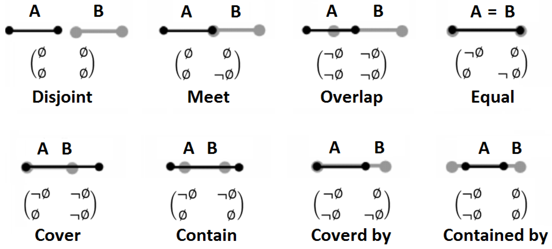
3.2. Topological Spatial Relationships

In order to investigate the topological relationships between the objects, diverse methods have been proposed so far. The four-intersection matrix is one of the most extensively applied in this context. This matrix is considered as a comprehensive model to report the binary topological spatial relationships between regions, lines, and points [45,46]. Based on this model, the topological relation ${\mathrm{R}}_{\mathrm{a},\mathrm{b}}$ between two linear objects A and B is characterized by the binary value (empty, non-empty) of the set intersection of A’s interior ($\mathrm{A}°$) and boundary ($\partial \mathrm{A}$), with the interior ($\mathrm{B}°$) and boundary ($\partial \mathrm{B}$) of B (Equation (1)):

$${\mathrm{R}}_{\mathrm{a},\mathrm{b}}=\left[\begin{array}{c}\partial A\cap \partial B \partial A\cap B°\\ A°\cap \partial B A°\cap B° \end{array}\right]$$

(1)

Figure 6 illustrates the possible relationships between two linear objects in a two-dimensional space based on this model.

3.3. Data Quality Elements

A large body of research has been conducted to evaluate the quality based on methods which involve comparing the VGI with a set of spatial information reference. In these studies, a number of elements have been used for quality and by comparing the reference data with the contributed ones, a quantitative estimation is calculated concerning these elements. International Organization for Standards [47] defines five quality elements: completeness, logical consistency, positional accuracy, temporal accuracy, and thematic accuracy. In this section, we provide an overview of the method used to estimate positional accuracy and completeness.

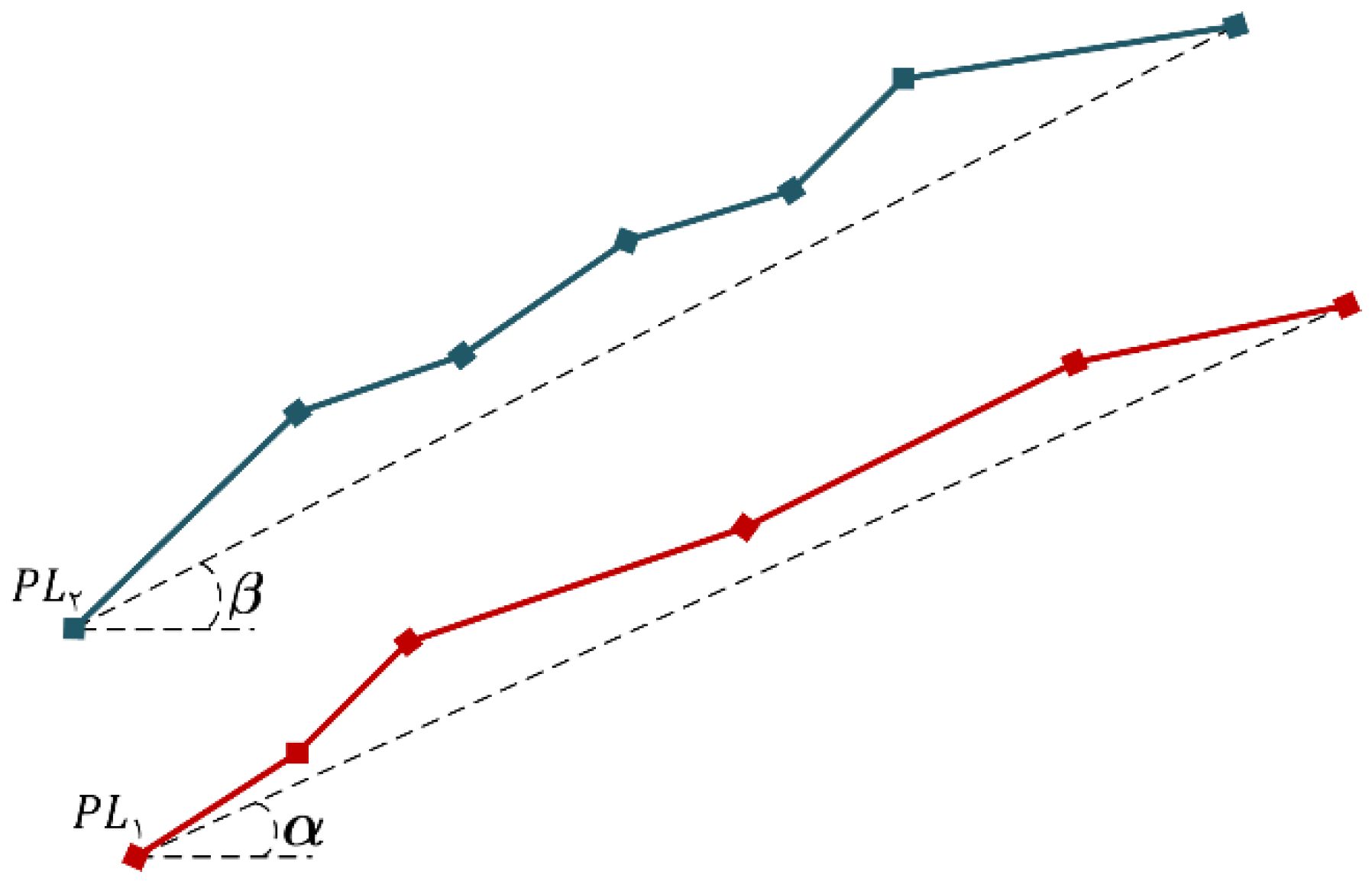
3.3.1. Positional Accuracy

In order to estimate the positional accuracy, the proximity between lines in OSM and the reference data is measured and compared. To do so, the following four criteria of Hausdorff distance, orientation, shape, and the overlapped buffer area are considered. For normalization of criteria, Chehreghan and Ali Abbaspour [48] have assessed fuzzy membership functions (Z-shape function) for checking similarity. The reason for doing so is that it is a suitable function for quantifying similarity and dissimilarity between the linear objects from two sources [48]. Hence, the positional accuracy for each object is computed using Equation (2):

$$Q_p=\frac{{\sum }_{i=1}^4{w}_i{c}_i}{{\sum }_{i=1}^4{w}_i}\times 100$$

(2)

where $Q_p$ represents the spatial similarity relation between the objects, and $w_i$ represents the weights given to the criterion. The values of the criteria are calculated after normalization by a membership function [48]. What follows is a description of the criteria being used:

Distance: One of relevant methods to estimate the distance in spatial sciences is the Hausdorff distance that estimates the closeness between the linear objects [49]. The Hausdorff distance has been introduced as the greatest distance between the shortest distance existing between each point from the first object and the set of the points of the second objects [50]. Nonetheless, the Hausdorff distance is sensitive to the shape of the two objects, especially to the parts far from the center. Tong et al. [51] introduced the short-line median Hausdorff distance (SMHD), indicating that, in comparison with Hausdorff and median Hausdorff, this method has a lower variance and a more efficient performance when facing complex data to measure the distance between the linear objects [52]. The SMHD between two linear objects can be calculated through Equation (3) where $L\left(P{L}_1\right)$ and $L\left(P{L}_2\right)$ are the length of the two linear objects, while $m\left(P{L}_1,P{L}_2\right)$ and $m\left(P{L}_2,P{L}_1\right)$ signify the median of the shortest distance between each point of the first object and the points of the corresponding object. These are calculated using Equations (4) and (5):

$$C_1=\{\begin{array}{c}m\left(P{L}_1,P{L}_2\right), if L\left(P{L}_1\right)<L\left(P{L}_2\right)\\ m\left(P{L}_2,P{L}_1\right), if L\left(P{L}_1\right)\ge L\left(P{L}_2\right)\end{array}$$

(3)

$$m\left(P{L}_1,P{L}_2\right)=media{n}_{P_a\in P{L}_1}\left\{mi{n}_{P_b\in P{L}_2}\left|\right|P_a-L_b\left|\right|\right\}$$

(4)

$$m\left(P{L}_2,P{L}_1\right)=media{n}_{P_b\in P{L}_2}\left\{mi{n}_{P_a\in P{L}_1}\left|\right|P_b-L_a\left|\right|\right\}$$

(5)

In these Equations, $L_b$ and $L_a$ are two edges of the linear objects $P{L}_1$ and $P{L}_2$, $P_a$ and $P_b$ are the points belonging to $P{L}_1$ and $P{L}_2$, respectively. $\left|\right|.\left|\right|$ denotes the Euclidean distance between a point on object and one of the edges of another object.

Orientation: This criterion is employed to compare the local orientation of two linear objects. The orientation difference between two linear objects can play a substantial role as a geometrical criterion in the evaluation of data quality [53]. The angle between the line formed from the beginning and ending points of the object and the horizontal axis determine the orientation of a linear object. See $P{L}_1$ and $P{L}_2$ in Figure 7, where two linear objects are considered to be parallel, while the angle difference of α and β is close to zero. In case the angle difference of the objects is close to π, it implies that these two linear objects are parallel, but have different orientations. The orientation difference between two linear objects can be estimated using Equation (6) [54]:

$$C_2={\cos }^{-1}\left(\frac{{\overrightarrow{V}}_{P{L}_1}.{\overrightarrow{V}}_{P{L}_2}}{{\overrightarrow{V}}_{P{L}_1}.{\overrightarrow{V}}_{P{L}_2}}\right)$$

(6)

where ${\overrightarrow{V}}_{P{L}_1}$ and ${\overrightarrow{V}}_{P{L}_2}$ are the vectors formed from the first and second nodes of the first and second objects.

Shape: The linear objects might vary in terms of shape so that the difference in the shape of two objects is used as another well-known criterion for the evaluation of the difference between two polylines (open or close). One of the functions related to the object shape is the cumulative angle function [55,56]. To calculate the shape difference between two linear objects, Equation (7) could be adopted in which ${\theta }_{P{L}_1}$ and ${\theta }_{P{L}_2}$ are the cumulative angle functions of the linear objects $P{L}_1$ and $P{L}_2$, respectively [54]:

$$C_3={\int }_0^{1}f\left({\theta }_{P{L}_1},{\theta }_{P{L}_2}\right)ds, f\left({\theta }_{P{L}_1},{\theta }_{P{L}_2}\right)=\{\begin{array}{c}\left|{\theta }_{P{L}_1}-{\theta }_{P{L}_2}\right|, if\left|{\theta }_{P{L}_1}-{\theta }_{P{L}_2}\right|\le \pi \\ 2\pi -\left|{\theta }_{P{L}_1}-{\theta }_{P{L}_2}\right|, if\left|{\theta }_{P{L}_1}-{\theta }_{P{L}_2}\right|>\pi \end{array}$$

(7)

3.3.2. Completeness

The road length is generally used to investigate the completeness of the OSM data in comparison with the reference data. In order to determine the completeness of a road network, the lengths of roads from the OSM are compared with the reference data. [57]. This metric is calculated as the ratio of the length of the OSM object (${\mathrm{L}}_{\mathrm{OSM}}$) to the length of the reference object (${\mathrm{L}}_{\mathrm{Ref}}$) in the same area using Equation (8) and presented as a percentage. The closer this ratio is to one-hundred, the more coverage of the OSM data is obtained:

$${\mathrm{Q}}_{\mathrm{C}}=\frac{{\mathrm{L}}_{\mathrm{OSM}}}{{\mathrm{L}}_{\mathrm{Ref}}}\times 100$$

(8)

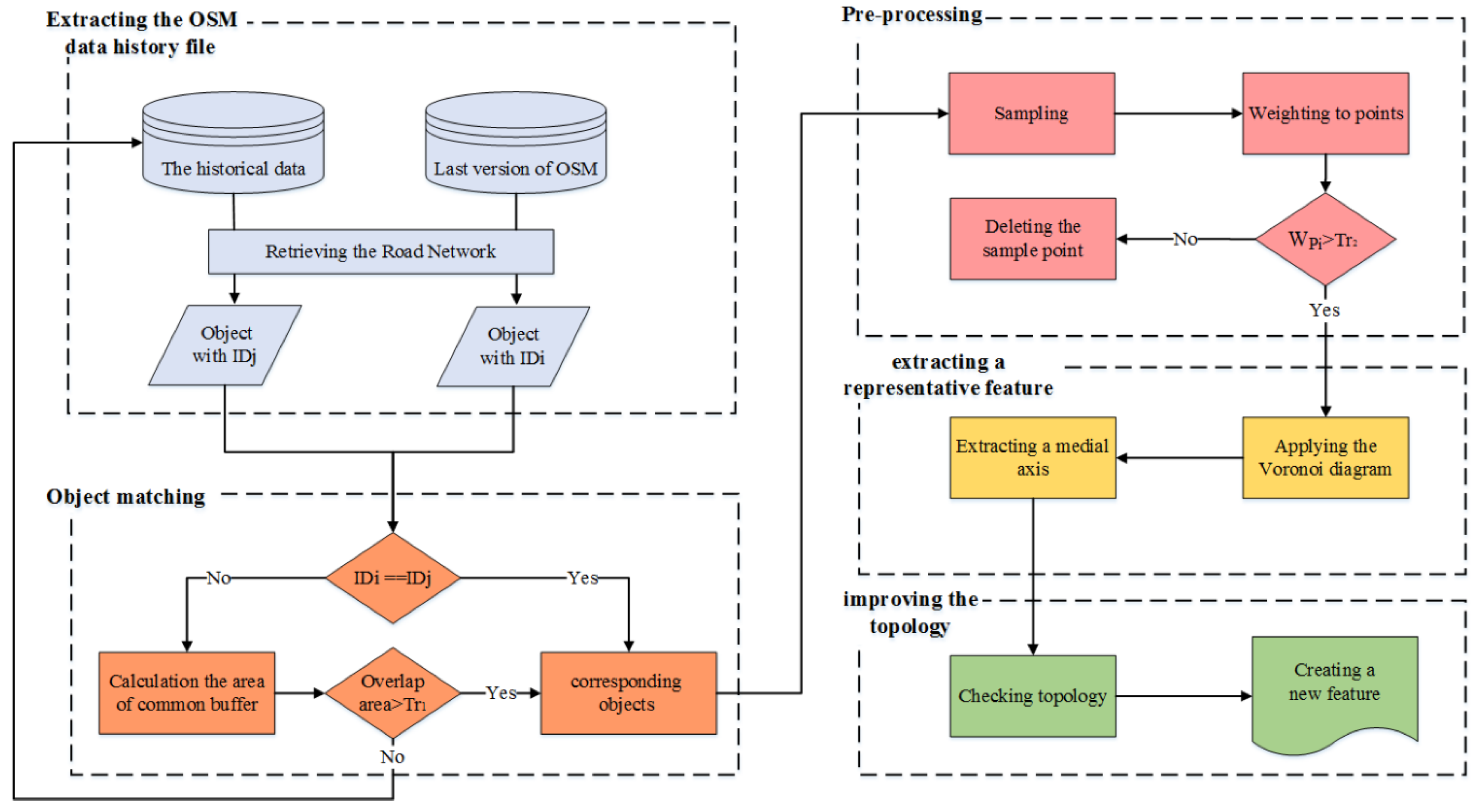
4. The Proposed Approach

Our method proposes an approach based on a Voronoi diagram for enhancing the positional accuracy of road network in OSM. The adopted method includes five stages, as shown in Figure 8. Restoring the historical versions of an object was a prerequisite in this research. With reference to this, during the first stage, the history file of the OSM data, which encompasses the entire information about all the OSM objects, had to be compiled. Having compiled the history file of Tehran, the information related to the latest version existing in OSM was also extracted. Afterwards, for each object in the latest version, the corresponding objects in all the existing versions in the history file were identified. To do so, two types of information, namely, semantic and geometric, related to the objects were used. During the third stage, after matching the corresponding objects, preprocessing was performed with the intention of identifying and removing the outlier data from the historical versions of each object. The fourth stage aimed at extracting a representative object for each object among all the existing versions. As such, we made use of the medial axis extraction method by implementing the Voronoi diagram. In the last stage, the topology of the extracted object for each category of the corresponding objects in the roads network was enhanced. To fulfill this, the objects in the extracted version are connected to each other by investigating the topology of the objects in the history file, and this may increase the certainty in the output version. What follows is an explanation of the method involved in identifying the corresponding objects in the history file (Section 4.1), as well as the method involved in the identification and removal of the outlier data (Section 4.2).

4.1. Object Matching

Object matching refers to the identification of the objects with an equivalent entity in several datasets [58,59,60,61]. The main aim of object matching was to identify the corresponding objects across historical versions in the OSM history file. In general, three aspects, such as semantic, topologic, and geometric, are considered for the object matching process based on which similarity of the objects is evaluated to identify the corresponding objects [62].

Thereafter, we identified the corresponding objects in the linear dataset using two types of semantic and geometric information of the objects through two stages. In the first stage, the semantic information attributed to the spatial data in OSM was used. Figure 9 shows the semantic information about a linear object, including the ID of the object, the type of the object (primary road, secondary road, etc.), the traffic route (one-way or not), and maximum speed, among others. In many cases, the semantic information related to an object varies in historical versions. This is because the producers of such data might have an improper understanding of a certain object or might only be able to diagnose and perceive limited aspects of a certain spatial object [9]. For example, many users might mistakenly label the road type (highway, trunk road, primary road, etc.). Therefore, the semantic information related to the OSM objects is often deficient, implying that a mere reliance on the semantic information for identification of the corresponding objects is not sufficient.

In the second stage, buffer analysis was conducted as a method to identify the corresponding objects. The common buffer area is the area overlapped between the regions resulted from the buffer created for two linear objects [63]. For example, in Figure 10, for identifying the corresponding objects with a different semantic label, the common buffer area was used.

Equation (9) was used in order to estimate the common buffer area of the objects, where $A_{P{L}_1}$ is the resultant buffer area for the first linear object, while $A_{P{L}_2}$ stands for the buffer area of the second linear object, and $A_i$ is the area of the region overlapped by the two resultant buffers. The closer the obtained results are to each other, the more similar the two objects are in terms of geometry:

$$C_4=\frac{2A_i}{A_{P{L}_1}+A_{P{L}_2}}$$

(9)

4.2. Identification and Removal of Outliers

The process involved in the identification and removal of the outlier data is typically done with a focus on the geometrical aspects of data and commonly includes techniques for cleansing data from errors. Due to the fact that all the versions and changes of a certain object was accessible, the criteria to choose the invalid object was the number of the repetition of an object’s spatial location. This process was performed in two stages (Figure 11). During the first stage, each linear object was converted into a point set using the sampling method. Using a sampling technique, we take the point between the two points of the linear object, except for the beginning and the end at specified intervals. In the second stage, the outlier data in the corresponding objects of a specific object are identified using density-based spatial clustering of applications with noise (DBSCAN) algorithm [64]. According to Algorithm 2, presented in Figure 11, each sample point is primarily weighted. Weighting is done based on the number of points in each point’s buffer, i.e., the points which are less than the radius (e.g., valued as 5 m in the experiments developed) would receive a significance degree and in case their significance is less than a certain threshold, they are considered as outliers and are consequently removed. If their weights go beyond the specified threshold, they will be retained in the main dataset.

5. Implementation

5.1. Case Studies

In this study, district 6 of Tehran’s municipality with about 21 km² area was selected for our investigation. For implementation, the suggested comprehensive file of the OSM history was extracted from http://planet.openstreetmap.org/ in the PBF format. To separate the history file of the chosen study area from the comprehensive file, osmconvert software (http://wiki.openstreetmap.org/wiki/Osmconvert) was used. The format of the history file was converted from PBF into OSM. In this file, there are different versions of the points, ways, and relations, respectively. We concentrated on enhancing the quality of the linear data and the linear data were separated from the history file. Figure 12a presents the history file of the study area while Figure 12b shows the latest version of the information about the objects existing in OSM. The users have used 24 labels to classify the streets in the study area. The objects having the following labels which include 37,238 objects that were investigated: motorway, trunk, primary, secondary, tertiary, and residential. In order to evaluate data quality, a reference dataset generated by Tehran Municipality at a cartographic scale of 1:2000 was used, as shown in Figure 12c. The OSM datasets were provided in the Geographical Coordinate System with the WGS-1984 reference ellipsoid, which was projected onto the UTM projection, zone 39.

5.2. Identification of the Corresponding Objects in the History File

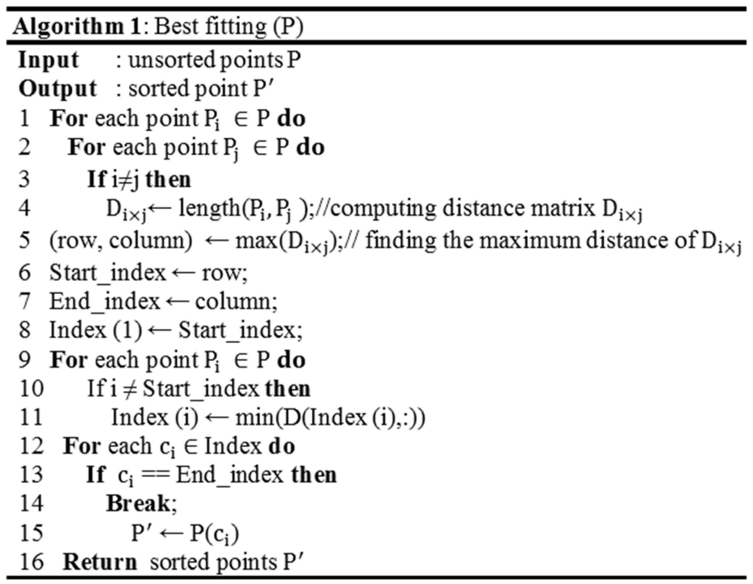
At this stage, at first the corresponding objects in the history file were identified; afterwards, of the corresponding objects of one object, a corresponding feature was produced for that object by extracting the medial axis. The complied history file includes the historical contributions of an object from 2007 to 2017.

Identifying the corresponding objects for each object in historical versions was conducted through two steps. In the first step, by investigating the semantic information in the history file, it became evident that the label of the object ID was identical in almost all versions of the changes of an object. For this reason, to identify the corresponding objects, the ID in the history file was used. For example, in Figure 13 for object L1 with ID 429262, object L2 was considered to be equivalent based on the same ID. The second step, which involves identifying the corresponding objects with a different semantic label, the common buffer area was used as the criterion. To fulfil this, for both linear objects, a buffer analysis with a distance of 10 m (valued in the experiments developed) corresponding to its width was created and the overlapping area of the two buffers is estimated. Equation (9) was employed to compute the objects common area. In case this value is larger than the threshold, the two objects could be identified as two corresponding objects.

5.3. Preprocessing

Since OSM data are retrieved with some topological errors, data preprocessing is important to minimize the possible outliers. The preprocessing encompasses the reduction and removal of the outliers from the spatial information. In practice, the geometric information of an object would be considered when identifying and removing the error from the historical versions of an object.

To eliminate the outlier data in the corresponding objects of a certain object, a point-based and two-stage solution was introduced in Section 3.2, during which, firstly, the set of the corresponding objects for each object was converted into points by sampling, while during the second stage the outlier data were identified and removed based on the predefined threshold using the DBSCAN method [65]. For instance, it is shown in Figure 14 that five points (${\mathrm{P}}_1$ to ${\mathrm{P}}_5$ with a weight less than 2) were identified as the outlier points and were, accordingly, removed from the set of the points. Having identified and removed the outlier points, the medial axis process was carried out on the data.

5.4. Extracting the Medial Axis

The aim of this stage was to extract a representative feature for an object among all the versions existing in the history file. Therefore, the method proposed in Section 3.1 was used to extract the medial axis. In the first stage, a buffer was created (e.g., valued as 10 m in the experiments developed) around the points sampled from each object (Figure 15a). In the second stage, the Delaunay triangulation of the set of points resultant from the buffer of the sampled points was formed (Figure 15b). In the third stage, the edges of the formed triangles in the Delaunay triangulation, which are determined from the object’s border, are removed (Figure 15c). In the fourth stage, after triangulation of the sampled points, the Voronoi diagram was created (Figure 15d). During the next stage, the Voronoi diagram vertices were extracted (Figure 15e). Finally, the diagrams vertices are connected and the medial axis is extracted using Algorithm 2 (Figure 15f).

However, it should be noted that a refinement stage was executed to simplify and smoothen the border of the buffer before estimating the medial axis because of the fact that the number of polygon points obtained from the buffer of the sampled points was high. After simplifying the boundary of the shape, the medial axis was extracted. The medial axis also had numerous details and nuances and the oversampling problem. Therefore, a post-processing step was required after calculating the medial axis to remove additional branches of the medial axis and maintain the main branches. In this study, two radial distance and perpendicular distance simplification algorithms were implemented. The radial distance algorithm eliminates the points in the vicinity of the specific radius, while the perpendicular distance algorithm is an iterative process so that a point among three points is removed, if the distance of the midpoint from the line passing from the other two points is less than the specified threshold value.

5.5. Topological Check of the Objects

At this stage, the topology of the object extracted for each of the corresponding objects in the road network has to be checked. The topological errors in the created version are eliminated by examining how the objects are connected to each other in the history of that object. Hence, the connections of each object to other objects were examined in the history file so that, for each object, every version was inspected to determine what type of topological relation they have with the other objects. A four-intersection topological model was used to determine the topological relationships between linear objects in a two-dimensional space. Using this model, the topological information of the dataset in the history file was extracted. The topological information extracted from the history, along with the type of their topological relationship, was recorded in a table. For example, in Figure 16, the topology relationships between the four versions of the L line and ${\mathrm{L}}_2$ line were marked and stored in a descriptive table. According to the table, the first version of the line L has a “disjoint” topological relationship with line ${\mathrm{L}}_2$; nonetheless, the other three versions, which also include the latest version of the site, have a “meet” topological relationship with ${\mathrm{L}}_2$ line. Since these data were recorded by contributors in OSM, the basis for recognizing the topological relationship between two linear objects was the number of repetitions of a topological relationship between the two objects in two editions of two object. According to the results of the descriptive table, it is expected that the two newly-created versions from the two linear objects L and ${\mathrm{L}}_2$ will have the “meet” topological relation.

After discovering the spatial relationships between the objects, it is necessary to correct the map and fix the errors. Two examples of common errors in the linear data are overshoot and undershoot errors, which both imply a lack of precise alignment of the lines in the connection spot. If any object encounters overshoot and undershoot errors, it is necessary to fix these errors. For example, in Figure 17, line L1 has an overshoot error, while L2 line has an undershoot error, in which the distances of overshoot and undershoot have to be resolved.

5.6. Evaluation of the Approach

The proposed method for improving the positional accuracy of the data exploits the inherent characteristics of the historical contributions (i.e., lineage) from multiple users. In Figure 18, several examples are displayed showing the objects, which were enhanced using our proposed approach. Linear objects are closer to the reference data in the compiled version, while having an enhanced quality compared to the latest version in OSM. Furthermore, we attempted to improve the topological relationships of the objects in the produced version by examining the topological relationships between the linear objects in the history file, which is shown in Figure 18.

In this study, two data quality elements, namely, completeness and positional accuracy, were estimated to evaluate the proposed method. To fulfil this, the quality of the latest version of the dataset in OSM and the dataset extracted by the proposed solution was determined based on the difference with the reference dataset.

The positional accuracy of the dataset was estimated, while the latest version of information of the object available in OSM, in comparison with the reference dataset, was created by calculating the geometric differences. Four criteria, such as distance, shape, orientation, and the common buffer area were considered to numerically evaluate the geometric quality of the objects and a weight of 0.62, 0.7, 0.31, and 0.65 was given to each of these parameters, respectively, as proposed by [48]. After calculating the effect of different parameters on the difference of the positional precision, Equation (2) was used to estimate the positional accuracy. The result obtained through this evaluation is illustrated in Figure 19. Our early findings confirm that the positional accuracy of OSM features can be improved through retrieving their historical contributions from OSM.

To evaluate the completeness, the typical approach of comparing the length of the two datasets was applied. Completeness of the dataset was determined by calculating the total length of the roads in the latest OSM version compared with the extracted dataset and, subsequently, compared with the reference map in the same area. The results obtained through these comparisons are exhibited in Figure 20, proving that the proposed method improved the completeness in the compiled version.

The evaluation results in Figure 19 and Figure 20 reveal that the proposed method has considerably enhanced the positional accuracy and completeness of OSM. Statistically speaking, the mean value of positional accuracy was enhanced from 82.5% to 95.3% using our proposed method. Additionally, from a completeness viewpoint, the completeness of roads in the study area was improved from 86.2% to 97.1% compared to the reference dataset. This implies that our proposed method can substantially reduce the quality differences between the raw OSM data and its reference dataset.

6. Discussion and Conclusions

OSM, as the most successful instance of VGI projects, offers numerous unique merits, in particular, retrieval of historical contributions. On the other hand, studies have proven that a larger number of contributors leads to better data quality in VGI based on the fact that data quality is better if more people get involved and contribute. However, there is a high probability that some contributors might reduce the quality of a given feature by eliminating some information around a feature. Therefore, the historical contributions should include some useful information for improving data quality. Hence, the current research was designed to propose an approach to improve the quality of the contributions in OSM through the long-term historical edits. In this study, all the historical edits from 2007 to 2017 were used to extract representative features for the street network of the study area. The choice of Tehran as a case study aimed at exploring the feasibility of the proposed approach in areas with limited contributors and the lack of a strong mapping community. Finally, the results of the study were evaluated against a high-quality reference dataset. The resultant maps and quality measures reveal that our approach was successful to enhance the positional accuracy and completeness of OSM data considerably while resolving topological errors.

The results prove the capability of the proposed method to improve the quality of VGI data. However, it should be noted that the results are sensitive to temporality of the contributions because, in a dynamic landscape, some features might have changed in the chosen timeframe, while the reference data may not have been updated accordingly. Therefore, the results of our approach, as well as the quality of the reference data, might have been biased by data temporality. Future studies should focus on determining the weights of OSM features based on their currency so that the latest contributions receive higher weights.

One of the unique strengths of OSM is the availability of historical edits, which allows us to see behind the scenes of contributions and how they have evolved over time. Therefore, the history of OSM contributions is certainly a rich resource for a number of purposes, including (a) tracking the quality of contributions over time in order to enhance the latest version; (b) monitoring changes across the landscape since the OSM life cycle exceeds 14 years so far; (c) subsequently, generating multi-temporal datasets instead of representing a static time; (d) mining users’ behaviors in mapping practices, i.e., what they map correctly and incorrectly; (e) how an object constantly remains persistent/edited over time; (f) historical completion of semantic/attribute information of objects; (g) cross-linking data quality with user behaviors and their socioeconomic history; and (h) ranking users’ activities in OSM. Future studies should focus on exploiting the history of objects towards addressing these issues.

Finally, the role of a number of contributors is evident while looking at historical edits for quality enhancement. However, this factor might still be challenging in some areas with inadequate contributors contributing to creating maps of that particular region. This is more crucial in developing countries with scarce mapping communities compared to active mapping communities across the globe. Thus, the OSM mapping communities should extend the mapping events and strengthen the motivating mechanisms for further user engagement across the globe.

References

1. Ballatore, A.; Jokar Arsanjani, J. Placing Wikimapia: An exploratory analysis. Int. J. Geogr. Inf. Sci. 2018, 32, 1–18. [Google Scholar] [CrossRef]
2. Hashemi, P.; Abbaspour, R.A. Assessment of logical consistency in OpenStreetMap based on the spatial similarity concept. In Openstreetmap in Giscience; Springer: Berlin, Germany, 2015; pp. 19–36. [Google Scholar]
3. Goetz, M. Towards generating highly detailed 3D CityGML models from OpenStreetMap. Int. J. Geogr. Inf. Sci. 2013, 27, 845–865. [Google Scholar] [CrossRef]
4. OSM Statistics. Available online: http://wiki.Openstreetmap.Org/wiki/stats (accessed on 24 June 2017).
5. Full History Dump. Available online: http://wiki.Openstreetmap.Org/wiki/planet.Osm/full (accessed on 23 June 2017).
6. Barron, C.; Neis, P.; Zipf, A. A comprehensive framework for intrinsic OpenStreetMap quality analysis. Trans. GIS 2014, 18, 877–895. [Google Scholar] [CrossRef]
7. Grira, J.; Bédard, Y.; Roche, S. Spatial data uncertainty in the VGI world: Going from consumer to producer. Geomatica 2010, 64, 61–72. [Google Scholar]
8. Feick, R.; Roche, S. Understanding the value of VGI. In Crowdsourcing Geographic Knowledge; Springer: Berlin, Germany, 2013; pp. 15–29. [Google Scholar]
9. De Longueville, B.; Ostländer, N.; Keskitalo, C. Addressing vagueness in volunteered geographic information (VGI)—A case study. Int. J. Spat. Data Infrastruct. Res. 2010, 5, 1725–0463. [Google Scholar]
10. Kounadi, O. Assessing the Quality of OpenStreetMap Data. Master’s Thesis, Geographical Information Science, Department of Civil, Environmental and Geomatic Engineering, University College of London, London, UK, 2009. [Google Scholar]
11. Girres, J.F.; Touya, G. Quality assessment of the french OpenStreetMap dataset. Trans. GIS 2010, 14, 435–459. [Google Scholar] [CrossRef]
12. Haklay, M. How good is volunteered geographical information? A comparative study of OpenStreetMap and ordnance survey datasets. Environ. Plan. B Plan. Des. 2010, 37, 682–703. [Google Scholar] [CrossRef]
13. Zielstra, D.; Zipf, A. A comparative study of proprietary geodata and volunteered geographic information for germany. In Proceedings of the 13th AGILE International Conference on Geographic Information Science, Guimaras, Portugal, 11–14 May 2010. [Google Scholar]
14. Neis, P.; Zielstra, D.; Zipf, A. The street network evolution of crowdsourced maps: Openstreetmap in germany 2007–2011. Future Internet 2011, 4, 1–21. [Google Scholar] [CrossRef]
15. Forghani, M.; Delavar, M.R. A quality study of the OpenStreetMap dataset for tehran. ISPRS Int. J. Geo-Inf. 2014, 3, 750–763. [Google Scholar] [CrossRef]
16. Arsanjani, J.J.; Mooney, P.; Zipf, A.; Schauss, A. Quality assessment of the contributed land use information from OpenStreetMap versus authoritative datasets. In Openstreetmap in Giscience; Springer: Berlin, Germany, 2015; pp. 37–58. [Google Scholar]
17. Mohammadi, N.; Malek, M. VGI and reference data correspondence based on location-orientation rotary descriptor and segment matching. Trans. GIS 2015, 19, 619–639. [Google Scholar] [CrossRef]
18. Lyu, H.; Sheng, Y.; Guo, N.; Huang, B.; Zhang, S. Geometric quality assessment of trajectory-generated VGI road networks based on the symmetric arc similarity. Trans. GIS 2017, 21, 984–1009. [Google Scholar] [CrossRef]
19. Brovelli, M.A.; Minghini, M.; Molinari, M.; Mooney, P. Towards an automated comparison of OpenStreetMap with authoritative road datasets. Trans. GIS 2017, 21, 191–206. [Google Scholar] [CrossRef]
20. Dorn, H.; Törnros, T.; Zipf, A. Quality evaluation of VGI using authoritative data—A comparison with land use data in Southern Germany. ISPRS Int. J. Geo-Inf. 2015, 4, 1657–1671. [Google Scholar] [CrossRef]
21. Arsanjani, J.J.; Barron, C.; Bakillah, M.; Helbich, M. Assessing the quality of OpenStreetMap contributors together with their contributions. In Proceedings of the AGILE, Vienna, Austria, 3–7 June 2013; pp. 14–17. [Google Scholar]
22. Haklay, M.; Basiouka, S.; Antoniou, V.; Ather, A. How many volunteers does it take to map an area well? The validity of linus’ law to volunteered geographic information. Cartogr. J. 2010, 47, 315–322. [Google Scholar] [CrossRef]
23. Leeuw, J.D.; Said, M.; Ortegah, L.; Nagda, S.; Georgiadou, Y.; DeBlois, M. An assessment of the accuracy of volunteered road map production in Western Kenya. Remote Sens. 2011, 3, 247–256. [Google Scholar] [CrossRef]
24. Neis, P.; Zipf, A. Analyzing the contributor activity of a volunteered geographic information project—The case of OpenStreetMap. ISPRS Int. J. Geo-Inf. 2012, 1, 146–165. [Google Scholar] [CrossRef]
25. Antoniou, V.; Touya, G.; Raimond, A.-M. Quality analysis of the parisian osm toponyms evolution. In European Handbook of Crowdsourced Geographic Information; Capineri, C., Haklay, M., Huang, H., Antoniou, V., Kettunen, J., Ostermann, F., Purves, R., Eds.; University of Zurich: Zurich, Switzerland, 2016; pp. 97–112. [Google Scholar]
26. Jonietz, D.; Zipf, A. Defining fitness-for-use for crowdsourced points of interest (POI). ISPRS Int. J. Geo-Inf. 2016, 5, 149. [Google Scholar] [CrossRef]
27. Keßler, C.; De Groot, R.T.A. Trust as a proxy measure for the quality of volunteered geographic information in the case of OpenStreetMap. In Geographic Information Science at the Heart of Europe; Springer: Berlin, Germany, 2013; pp. 21–37. [Google Scholar]
28. Keßler, C.; Trame, J.; Kauppinen, T. Tracking editing processes in volunteered geographic information: The case of OpenStreetMap. In Proceedings of the Workshop on Identifying Objects, Processes and Events in Spatio-Temporally Distributed Data (IOPE 2011), Belfast, ME, USA, 12–16 September 2011. [Google Scholar]
29. Rehrl, K.; Gröchenig, S. A framework for data-centric analysis of mapping activity in the context of volunteered geographic information. ISPRS Int. J. Geo-Inf. 2016, 5, 37. [Google Scholar] [CrossRef]
30. Sehra, S.S.; Singh, J.; Rai, H.S. Assessing OpenStreetMap data using intrinsic quality indicators: An extension to the qgis processing toolbox. Future Internet 2017, 9, 15. [Google Scholar] [CrossRef]
31. D’Antonio, F.; Fogliaroni, P.; Kauppinen, T. VGI edit history reveals data trustworthiness and user reputation. In Proceedings of the AGILE 2014, Castellón, Spain, 3–6 June 2014. [Google Scholar]
32. Touya, G.; Antoniou, V.; Olteanu-Raimond, A.-M.; Van Damme, M.-D. Assessing crowdsourced poi quality: Combining methods based on reference data, history, and spatial relations. ISPRS Int. J. Geo-Inf. 2017, 6, 80. [Google Scholar] [CrossRef]
33. Van Exel, M.; Dias, E.; Fruijtier, S. In The impact of crowdsourcing on spatial data quality indicators. In Proceedings of the 6th GIScience International Conference on Geographic Information Science, Zurich, Switzerland, 14–17 September 2010; p. 213. [Google Scholar]
34. Mooney, P.; Corcoran, P. Characteristics of heavily edited objects in OpenStreetMap. Future Internet 2012, 4, 285–305. [Google Scholar] [CrossRef]
35. Wiki. Available online: http://wiki.Openstreetmap.Org/wiki/planet.Osm (accessed on 25 July 2017).
36. Blum, H. A transformation for extracting descriptors of shape. In Models for the Perception of Speech and Visual Form; MIT Press: Cambridge, MA, USA, 1967. [Google Scholar]
37. Blum, H.; Nagel, R.N. Shape description using weighted symmetric axis features. Pattern Recognit. 1978, 10, 167–180. [Google Scholar] [CrossRef]
38. Attali, D.; Boissonnat, J.-D.; Edelsbrunner, H. Stability and computation of medial axes-a state-of-the-art report. In Mathematical Foundations of Scientific Visualization, Computer Graphics, and Massive Data Exploration; Springer: Berlin, Germany, 2009; pp. 109–125. [Google Scholar]
39. Armstrong, C.G. Modelling requirements for finite-element analysis. Comput. Aided Des. 1994, 26, 573–578. [Google Scholar] [CrossRef]
40. Hisada, M.; Belyaev, A.G.; Kunii, T.L. A skeleton-based approach for detection of perceptually salient features on polygonal surfaces. In Computer Graphics Forum; Wiley Online Library: Hoboken, NJ, USA, 2002; pp. 689–700. [Google Scholar]
41. Brandt, J.W.; Jain, A.K.; Algazi, V.R. Medial axis representation and encoding of scanned documents. J. Vis. Comm. Image Represent. 1991, 2, 151–165. [Google Scholar] [CrossRef]
42. Gold, C.; Dakowicz, M. The crust and skeleton—Applications in GIS. In Proceedings of the 2nd International Symposium on Voronoi Diagrams in Science and Engineering, Seoul, Korea, 10–13 October 2005; pp. 33–42. [Google Scholar]
43. Xia, H.; Tucker, P.G. Fast equal and biased distance fields for medial axis transform with meshing in mind. Appl. Math. Model. 2011, 35, 5804–5819. [Google Scholar] [CrossRef]
44. Cheng, S.-W.; Funke, S.; Golin, M.; Kumar, P.; Poon, S.-H.; Ramos, E. Curve reconstruction from noisy samples. Comput. Geom. 2005, 31, 63–100. [Google Scholar] [CrossRef]
45. Egenhofer, M.J.; Herring, J. Categorizing Binary Topological Relations between Regions, Lines, and Points in Geographic Databases; Technical Report; Department of Surveying Engineering, University of Maine: Orono, ME, USA, 1991. [Google Scholar]
46. Egenhofer, M.J.; Franzosa, R.D. Point-set topological spatial relations. Int. J. Geogr. Inf. Syst. 1991, 5, 161–174. [Google Scholar] [CrossRef] [Green Version]
47. ISO 19157:2013: Geographic information—Data Quality; International Organization for Standardization (ISO): Geneva, Switzerland, 2013.
48. Chehreghan, A.; Ali Abbaspour, R. An assessment of spatial similarity degree between polylines on multi-scale, multi-source maps. Geocarto Int. 2017, 32, 471–487. [Google Scholar] [CrossRef]
49. Abbas, I. Base de Données Vectorielles et Erreur Cartographique: Problèmes Posés par le Contrôle Ponctuel, une Méthode Alternative Fondée sur la Distance de Hausdorff: Le Contrôle Linéaire; ABES: Montpellier, France, 1994. [Google Scholar]
50. Li, L.; Goodchild, M.F. An optimisation model for linear feature matching in geographical data conflation. Int. J. Image Data Fusion 2011, 2, 309–328. [Google Scholar] [CrossRef]
51. Tong, X.; Liang, D.; Jin, Y. A linear road object matching method for conflation based on optimization and logistic regression. Int. J. Geogr. Inf. Sci. 2014, 28, 824–846. [Google Scholar] [CrossRef]
52. Chehreghan, A.; Ali Abbaspour, R. An assessment of the efficiency of spatial distances in linear object matching on multi-scale, multi-source maps. Int. J. Geogr. Inf. Sci. 2017, 1–20. [Google Scholar] [CrossRef]
53. Olteanu Raimond, A.-M.; Mustière, S. Data matching—A matter of belief. In Headway in Spatial Data Handling; Springer: Berlin, Germany, 2008; pp. 501–519. [Google Scholar]
54. Zhang, M. Methods and Implementations of Road-Network Matching. Ph.D. Dissertation, Technical University of Munich, Munich, Germany, 2009. [Google Scholar]
55. Veltkamp, R.C. Shape matching: Similarity measures and algorithms. In Proceedings of the International Conference onShape Modeling and Applications, Herzliya, Israel, 22–24 June 2001; IEEE: Piscataway, NJ, USA, 2001; pp. 188–197. [Google Scholar]
56. Ali Abbaspour, R.; Chehreghan, A.; Karimi, A. Assessing the efficiency of shape-based functions and descriptors in multi-scale matching of linear objects. Geocarto Int. 2017, 33, 1–14. [Google Scholar] [CrossRef]
57. Wang, M.; Li, Q.; Hu, Q.; Zhou, M. Quality analysis of OpenStreetMap data. ISPRS Int. Arch. Photogramm. Remote Sens. Spat. Inf. Sci. 2013, 2, W1. [Google Scholar]
58. Samal, A.; Seth, S.; Cueto, K. A feature-based approach to conflation of geospatial sources. Int. J. Geogr. Inf. Sci. 2004, 18, 459–489. [Google Scholar] [CrossRef]
59. Chehreghan, A.; Ali Abbaspour, R. A geometric-based approach for road matching on multi-scale datasets using a genetic algorithm. Cartogr. Geogr. Inf. Sci. 2017, 1–15. [Google Scholar] [CrossRef]
60. Chehreghan, A.; Ali Abbaspour, R. A new descriptor for improving geometric-based matching of linear objects on multi-scale datasets. GISci. Remote Sens. 2017, 54, 836–861. [Google Scholar] [CrossRef]
61. Dehghani, A.; Chehreghan, A.; Ali Abbaspour, R. Matching of urban pathways in a multi-scale database using fuzzy reasoning. Geod. Cartogr. 2017, 43, 92–104. [Google Scholar] [CrossRef]
62. Mustière, S.; Devogele, T. Matching networks with different levels of detail. GeoInformatica 2008, 12, 435–453. [Google Scholar] [CrossRef]
63. Fan, H.; Yang, B.; Zipf, A.; Rousell, A. A polygon-based approach for matching OpenStreetMap road networks with regional transit authority data. Int. J. Geogr. Inf. Sci. 2016, 30, 748–764. [Google Scholar] [CrossRef]
64. Ester, M.; Kriegel, H.-P.; Sander, J.; Xu, X. A density-based algorithm for discovering clusters in large spatial databases with noise. In Proceedings of the Knowledge Discovery and Data Mining, Portland, OR, USA, 2–4 August 1996; pp. 226–231. [Google Scholar]
65. Han, J.; Kamber, M.; Pei, J. Data Mining: Concepts and Techniques: Concepts and Techniques; Elsevier: New York, NY, USA, 2011. [Google Scholar]
Figure 1. Categorization of VGI quality assessment methods.
Ijgi 07 00253 g001
Figure 2. Category of information in the OSM history file.
Ijgi 07 00253 g002
Figure 3. (a) A part of the street network from OSM of Tehran; (b) a sample of the OSM history file for Sepand Street (yellow line) in version 1.
Ijgi 07 00253 g003
Figure 4. Medial axis for a 2D curve (adapted from [43]).
Ijgi 07 00253 g004
Figure 5. Pseudo-code representing Algorithm 1.
Ijgi 07 00253 g005
Figure 6. Eight kinds of topological relations for lines in a two-dimensional space [46].
Ijgi 07 00253 g006
Figure 7. Orientation difference between two linear objects.
Ijgi 07 00253 g007
Figure 8. Flowchart of the implementation of the proposed method.
Ijgi 07 00253 g008
Figure 9. An example of tags of Mirza Shirazi Street in OSM.
Ijgi 07 00253 g009
Figure 10. An example of the buffer method.
Ijgi 07 00253 g010
Figure 11. Pseudo-code depicting Algorithm 2.
Ijgi 07 00253 g011
Figure 12. Study area: (a) the OSM data history file; (b) the latest version of the OSM; and (c) the reference dataset.
Ijgi 07 00253 g012
Figure 13. An example of identifying the corresponding objects: (a) using the ID in the history file; and (b) calculating the common buffer area.
Ijgi 07 00253 g013
Figure 14. An example of identifying outlier points in all versions of an object.
Ijgi 07 00253 g014
Figure 15. The medial axis approximation using the Voronoi diagram method: (a) a sample point of the shape boundary; (b) Delaunay triangulation of the boundary points; (c) discarding triangles that are outside the shape; (d) applying the Voronoi diagram; (e) extracting the Voronoi diagram vertices; and (f) connecting the Voronoi diagram’s vertices based on Algorithm 2.
Ijgi 07 00253 g015
Figure 16. An example of the topology relationships between two linear objects.
Ijgi 07 00253 g016
Figure 17. Overshoot and undershoot errors.
Ijgi 07 00253 g017
Figure 18. An example of a reference dataset, the latest version of OSM, and extracted datasets.
Ijgi 07 00253 g018
Figure 19. (a) The computed positional accuracy of the latest version of OSM dataset; and (b) the computed positional accuracy of the enhanced dataset.
Ijgi 07 00253 g019
Figure 20. (a) Length percentage of the latest version of the OSM dataset; and (b) the length percentage of the enhanced dataset.
Ijgi 07 00253 g020