Change Detection for Building Footprints with Different Levels of Detail Using Combined Shape and Pattern Analysis

Abstract

Crowd-sourced geographic information is becoming increasingly available, providing diverse and timely sources for updating existing spatial databases to facilitate urban studies, geoinformatics, and real estate practices. However, the discrepancies between heterogeneous datasets present challenges for automated change detection. In this paper, we identify important measurable factors to account for issues like boundary mismatch, large offset, and discrepancies in the levels of detail between the more current and to-be-updated datasets. These factors are organized into rule sets that include data matching, merge of the many-to-many correspondence, controlled displacement, shape similarity, morphology of difference parts, and the building pattern constraint. We tested our approach against OpenStreetMap and a Dutch topographic dataset (TOP10NL). By removing or adding some components, the results show that our approach (accuracy = 0.90) significantly outperformed a basic geometric method (0.77), commonly used in previous studies, implying a more reliable change detection in realistic update scenarios. We further found that distinguishing between small and large buildings was a useful heuristic in creating the rules.

1. Introduction

Crowd-sourced geographic data, such as OpenStreetMap (OSM), are collected at an unprecedented speed and updated every minute. Besides the known problems in data quality [1,2], such data sources can be used as timely sources for change detection and incremental update. It is important to keep data (e.g., buildings and roads) up-to-date for domains like urban studies and management, geoinformatics, and real estate practices. On the other hand, professional geographical data, such as those maintained at national mapping agencies (NMAs), are usually not updated as quickly. For example, topographic data in Kadaster, the Netherlands are revised every two years [3], possibly because of its full coverage update policy. Commercial data providers usually have a quarterly update cycle for their navigation and points of interest (POI) data. This can lead to a situation where, though claimed to have better quality, professional data in many countries may always be outdated compared with their crowd-sourced counterparts, at least in locations such as urban areas [4,5]. It is, therefore, reasonable to combine the strengths of both sides. For example, by employing continuous revision methods, Ordnance Survey, United Kingdom has shortened the updating cycle of their OS MasterMap Topography Layer to six weeks. For example, see https://www.ordnancesurvey.co.uk/business-and-government/products/topography-layer.html. Automated change detection is thus important for a continuous and incremental update mechanism.

However, comparing heterogeneous data sources maintained by different organizations, such as OSM and professional providers, and detecting the changes with reasonable accuracy, is not a trivial task. There are three main issues that make this process challenging. First, heterogeneous spatial data can be different in their capture scale, leading to the boundary mismatch issue, which complicates the change comparison. For crowd-sourced data like OSM, levels of detail (LOD) can vary from object to object [6]. Second, the presence of many-to-many correspondences between datasets can further complicate the change detection. Third, change detection usually involves many parameters that are sensitive to small variations in position, shape, and LOD. As a result, the discrepancies observed between any two datasets can have different origins, and not all of them are physical changes.

In this paper, we focus on the building feature, as it is one of the most frequently updated features in map production [7]. Here, we aim to identify the measurable factors that are important for distinguishing real changes from other types of discrepancies, and to propose appropriate techniques for measuring and quantifying these factors for more reliable change detection. In the next section, we review related concepts and previous work on change detection, and elaborate more on the above-mentioned challenges.

1.1. Related Concepts and Issues in Change Detection

1.1.1. Nature of Changes

Many reasons explain the discrepancies between two data sets:

(1)

Data acquisition: Positional discrepancies could be the result of varying accuracy, resolution, and so on in data capture. Some objects might be deliberately omitted during data acquisition for certain purposes.

(2)

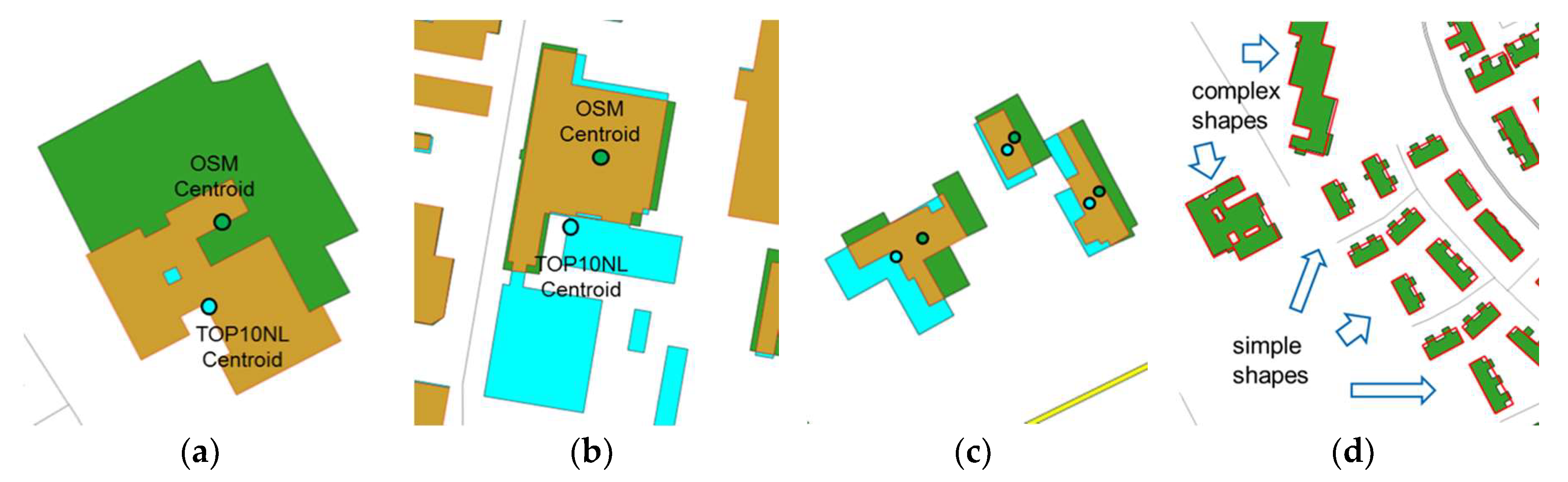
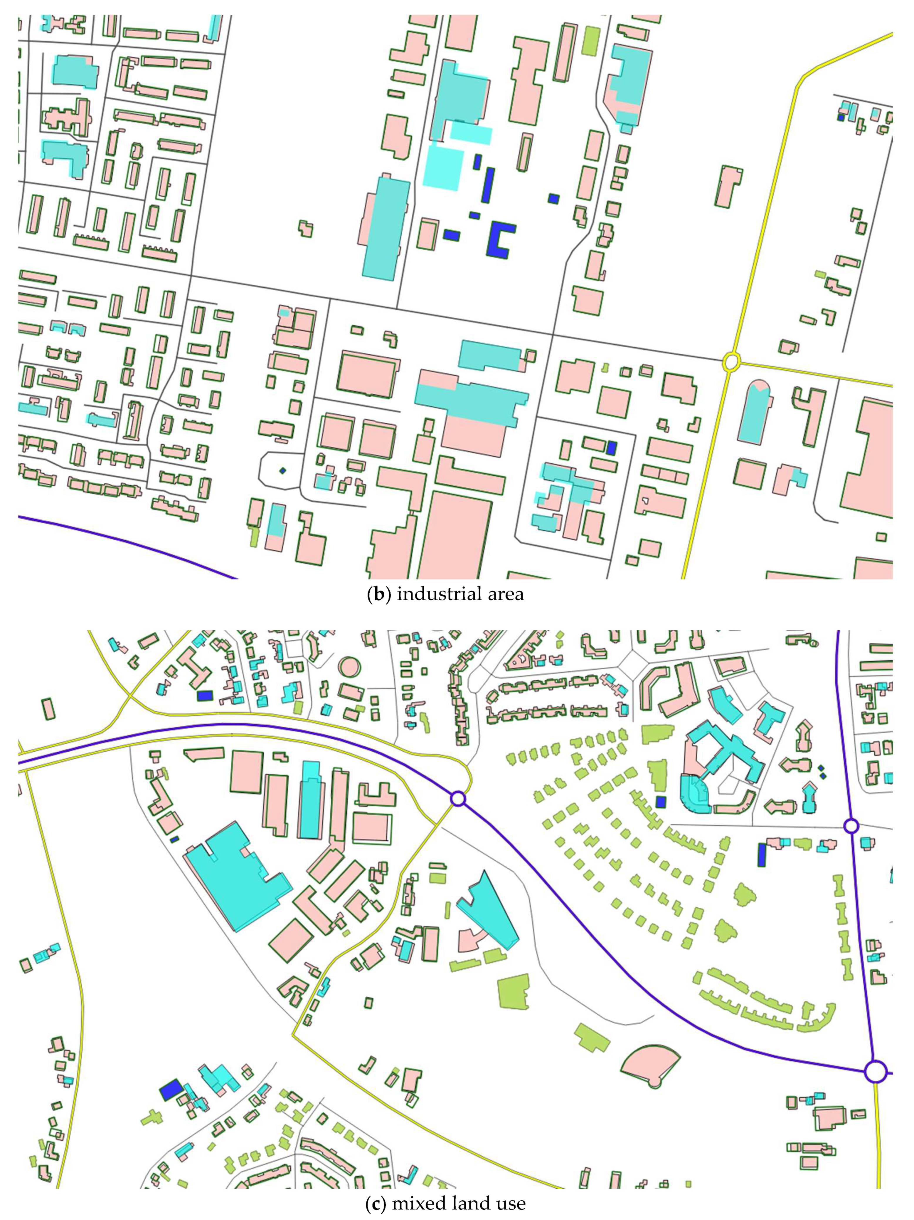
Data specifications: By comparison with high-resolution images, we found that OSM buildings with greater details were outlined by including the main building and annexes such as fences, courtyards, and garages, whereas in topographic datasets, mainly building roofs were recorded (Figure 1).

(3)

Generalization (or LOD): Objects can be simplified, displaced, aggregated, or typified during generalization, which creates apparent discrepancies between data representations.

(4)

Physical and nominal changes: The discrepancies due to real world changes to the construction itself (e.g., new construction, removal, and partial rebuilt) or to its semantics (e.g., land-use type, name, etc.)

The question is the following: can we distinguish real changes from other data discrepancies?

1.1.2. Previous Work and Issues in Change Detection

Most recent change detection literature is found in the remote sensing domain, which is motivated by updating existing databases [8,9]. Several researchers noted the importance of using vector data in image-based change analysis [10,11]. For example, Matikainen et al. [8] first extracted building footprints from images, which were then compared with old map data by overlapping two vector layers. The relative sizes of the overlap and difference areas were commonly used to determine the change in these methods. We show that this is not adequate in more general cases where map scale and map generalization can complicate the change analysis. Bouziani et al. [10] also noted that map generalization of building outlines affects change detection, and should be considered to improve their method.

As an alternative, updating existing databases from more current vector data has been a long-standing active topic in geoinformatics [12,13,14]. When comparing vector datasets, the map scale issue becomes even more important. This is especially true when updates are to be propagated to existing data maintained at multiple scales [15,16]. To this end, Yang et al. [17] proposed a map algebra-based technique for change detection and update in a multi-scale setting. Their method can handle the deviations in LOD, but assumes that the more current data is produced by the same provider so that no large offset exist between datasets. Furthermore, spatial data maintained at multiple scales should be updated while maintaining data consistency for map production and display [18]. This requires changes to be accurately detected at a larger scale and then propagated to smaller scales [19].

To summarize, the reviewed work on change detection with vector datasets seems to assume that more current and to-be-updated datasets are free from the boundary mismatch problem, excluding more practical needs of integrating updates from heterogeneous sources. Actually, updating from crowd-sourced geographic information has become more demanding in recent years [7], and the sources of update range from mobility tracks [20] to OSM [19,21]. Therefore, the more challenging problem of change detection from heterogeneous datasets needs to be further studied.

To be specific, crowd-sourced geographic information does not usually have an explicitly defined scale, and thus creates many problems in its use [6]. In the case of OSM, researchers have estimated its positional accuracy and equivalent reference scale, which is approximately 1:10,000 [7]. For building footprints in particular, the levels of detail are similar or with more details in general, but can be heterogeneous across the space [22].

Basic geometric analyses, such as the size of the buildings and that of their overlapping differences, are not adequate in more complicated situations (Figure 1). In all cases, we observed discrepancies in the LOD of the two datasets, even though their capture scales were similar. For example, comparison of building outlines can be complicated by the boundary mismatch problem (Figure 1a). Such discrepancies may also be caused by data acquisition, specification, or generalization (e.g., simplification and displacement), making it hard to distinguish them from physical changes. Overlaying the two datasets creates fragmented polygons (i.e., A-B, B-A, and A∩B). Analyzing the fragmented polygons using size alone is problematic (Figure 1b). For instance, N would also be regarded as a modified building (Figure 1f), which it is not, though the size of the fragmented polygon is larger than that of M (a real change). Furthermore, the offsets between the two data sets are not systematic (Figure 1), which cannot be rectified by geo-referencing. The same set of parameters is not suitable for detecting changes in all situations.

In addition, decisions based solely on information at the individual level can be sensitive to the above-mentioned small geometric variations, which may lead to inconsistent results. For example, detected changes in Figure 1h are hardly true because detached houses in the residential area seldom change in this minor and inconsistent way; they are usually either rebuilt or remain untouched. The apparent discrepancies may be the result of different specifications or generalization during data acquisition. No matter how we tune the parameters, we cannot obtain consistent results. Nevertheless, we note that some of the inconsistencies can be corrected by further incorporating semantics, functions, and patterns of the objects, where domain knowledge is relevant. Change detection with too many false positives would be useless for incremental update and understanding the dynamics of the land use change.

To overcome the above-mentioned difficulties, we present techniques that compare buildings in two data sets, and discover data discrepancies that are more likely caused by physical changes to the objects rather than by other causes. In particular, we compare OSM buildings with professional topographic data at 1:10,000 (TOP10NL), and identify changes for future updating and dynamic analysis.

This paper contributes to change detection and differs from previous methods. First, the many-to-many correspondence [19,23] is carefully dealt with in our approach, which should be able to leave out discrepancies by aggregation of buildings. Second, we propose a controlled alignment to alleviate the boundary mismatch problem. Third, we propose a new measure of the morphology of difference parts, which outperforms the basic size-based analysis and improves the accuracy. Finally, we propose using the knowledge of building patterns to constrain the detected changes and to reduce inconsistencies in the results.

2. Methodology

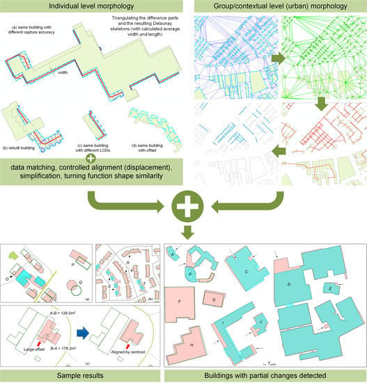
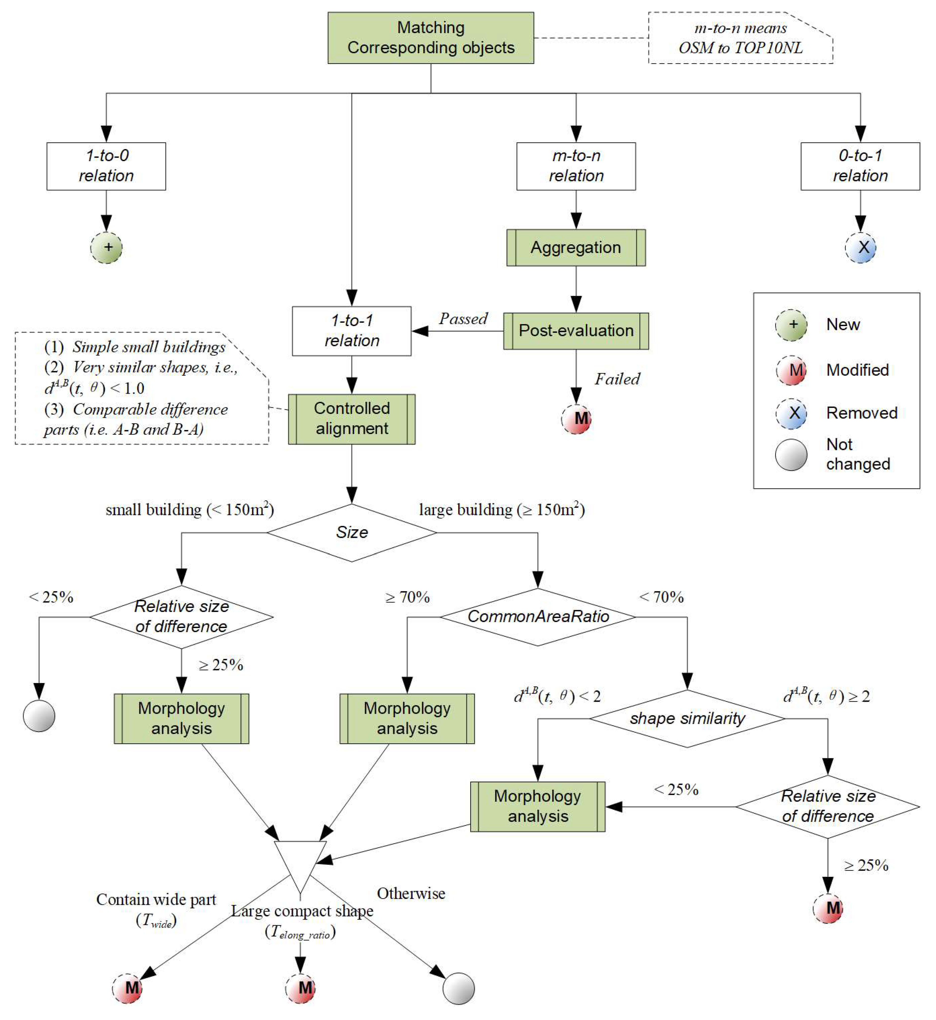
2.1. Overall Process

The general workflow is described as follows:

• Identifying corresponding objects between two datasets (Section 2.2). We aim to identify objects (or a group of objects) in the two datasets that correspond to each other, which is a prerequisite for the subsequent analysis.
• Rule-based change detection (Section 2.3). During this stage, change detection is carried out at the individual level (i.e., building footprints) using different rules and analysis proposed in this paper.
• Refining results with patterns and contextual information (Section 2.4). In this stage, we show how inconsistent results in change detection can be corrected using the building pattern constraint.

2.2. Object Matching

The first step in our approach is relatively easy. As a preprocessing step, we merged adjacent buildings of the same type (e.g., house, apartment, retail, etc.) in OSM, so that the polygons were more comparable in size to our TOP10NL dataset. As we assumed that the datasets to be compared were of similar scales or LOD to maximize the reliability of change detection, we used an overlap-based analysis to identify the correspondence between individual objects in the two datasets (see also [19]). Although offsets can be expected between small buildings, the offsets are relatively small for large buildings (Figure 1). We found that the ratio between the overlapped/common area and the original areas, that is, Equation (1), worked well for our matching problem. If one of the ratios was larger than, for example, 15%, we identified the pair as a corresponding relation. Although Rutzinger et al. [24] found a ratio of 30% useful in their cases (see also [5]), we had to lower this ratio to account for the sometimes large offset between corresponding objects in our datasets (Section 3.2.2).

CommonAreaRatio(x) = Area(A∩B)/Area(x), x ∈ {A, B},

(1)

Some identified corresponding relations are shown in Figure 2. Many-to-many corresponding relations [23] are still anticipated between datasets of similar scales. Formally, the resultant corresponding relations have the following cardinality: m-to-n (where m ≥ 1, n ≥ 1, m ≠ n, m indicates the number of objects in OSM and n indicates the number of objects in our data), 1-to-1, 1-to-0 (i.e., new objects in OSM), and 0-to-1 relations (objects in our data being teared down). We describe how the change detection procedure works in the following section.

2.3. Rules for Change Detection

We used rule-based change detection in our study, which combines evidence from different similarity measures and analysis. We found that distinguishing between large buildings (industrial, institutional building, or some street block polygons) and small ones (e.g., houses) in setting the rules and parameters proved to be useful heuristics (Section 2.3.3). First, we introduce the factors identified to address the aforementioned issues. These fall into the following basic categories:

(1)

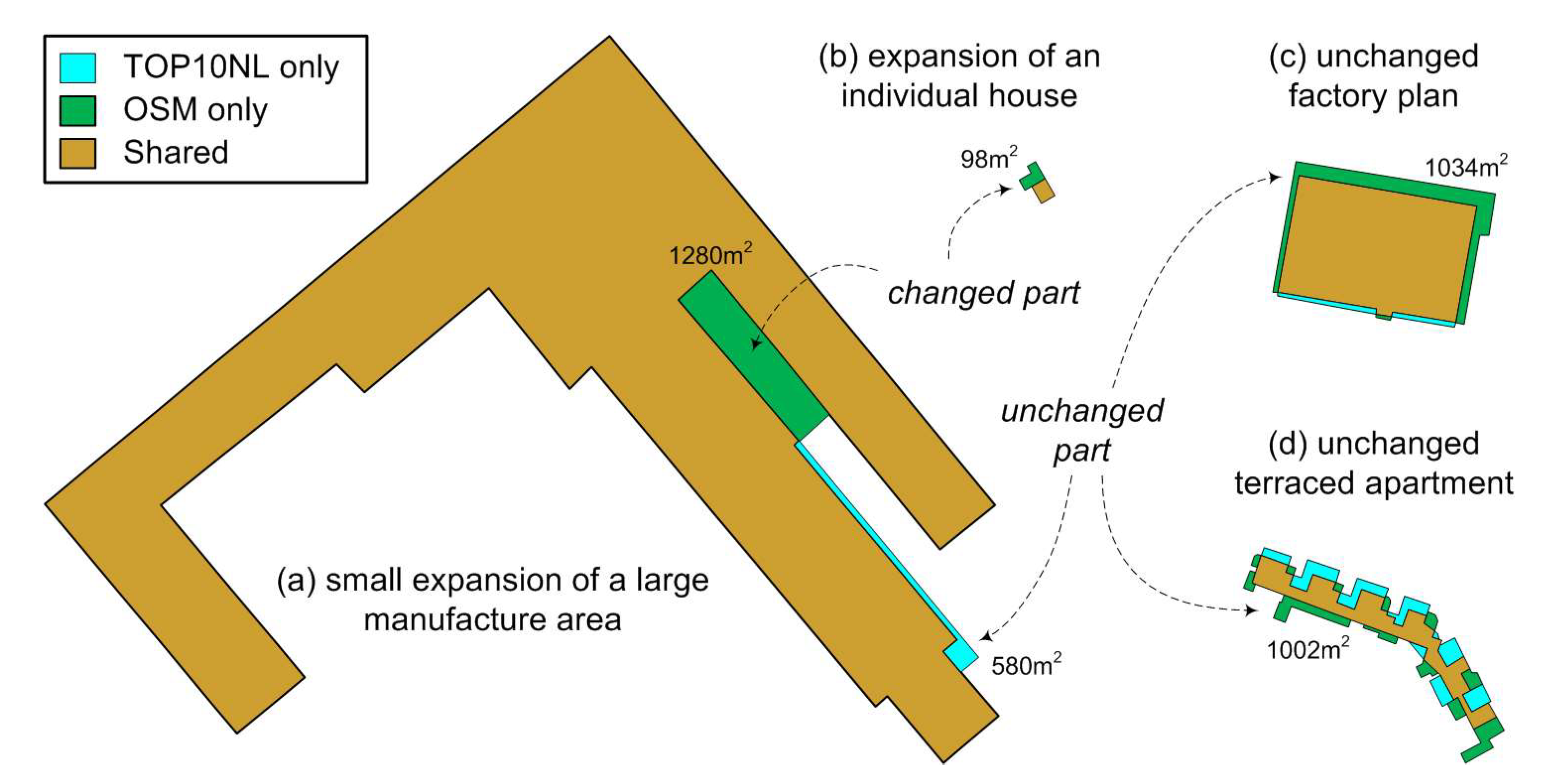
Absolute and relative size of the differences.

(2)

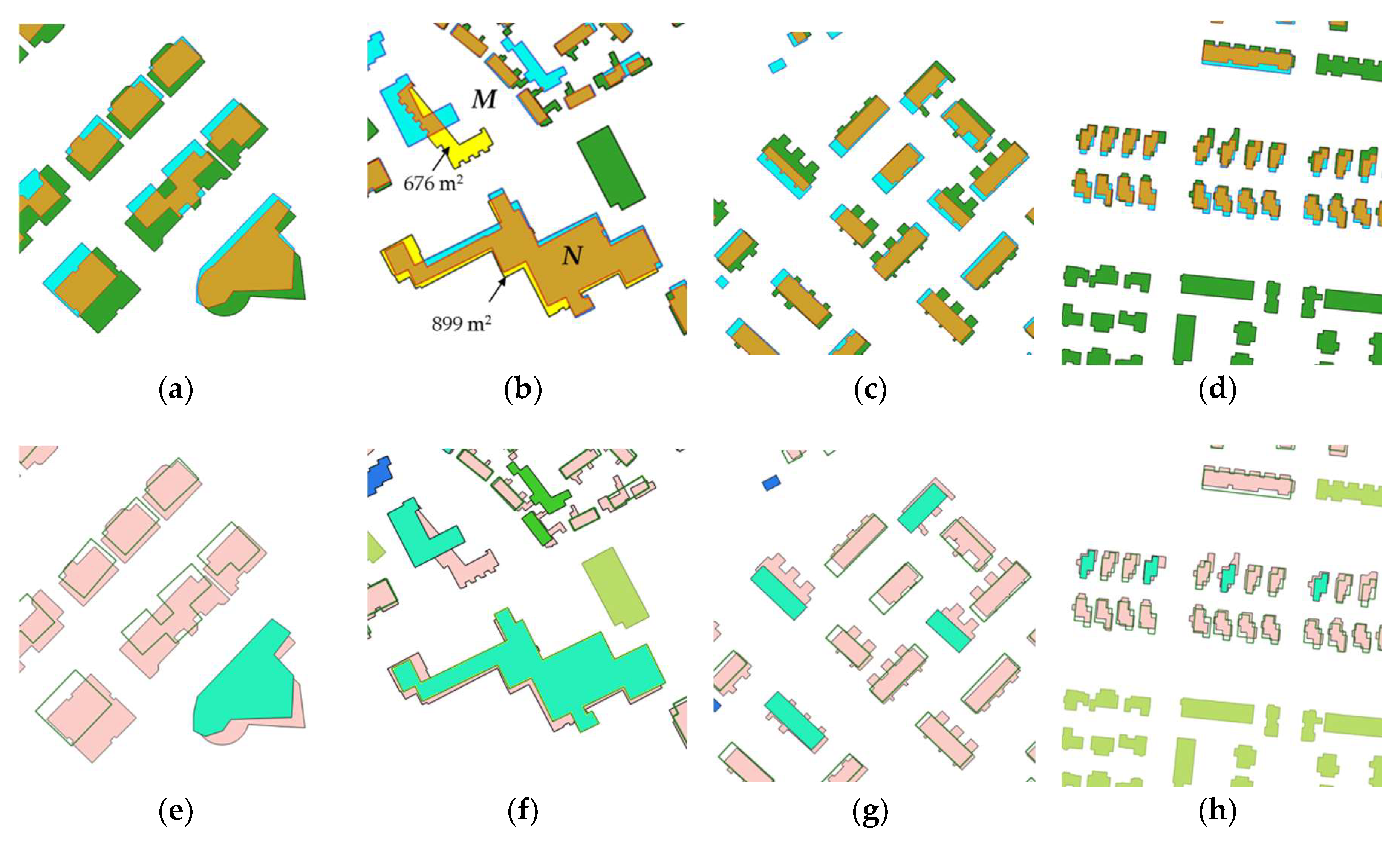
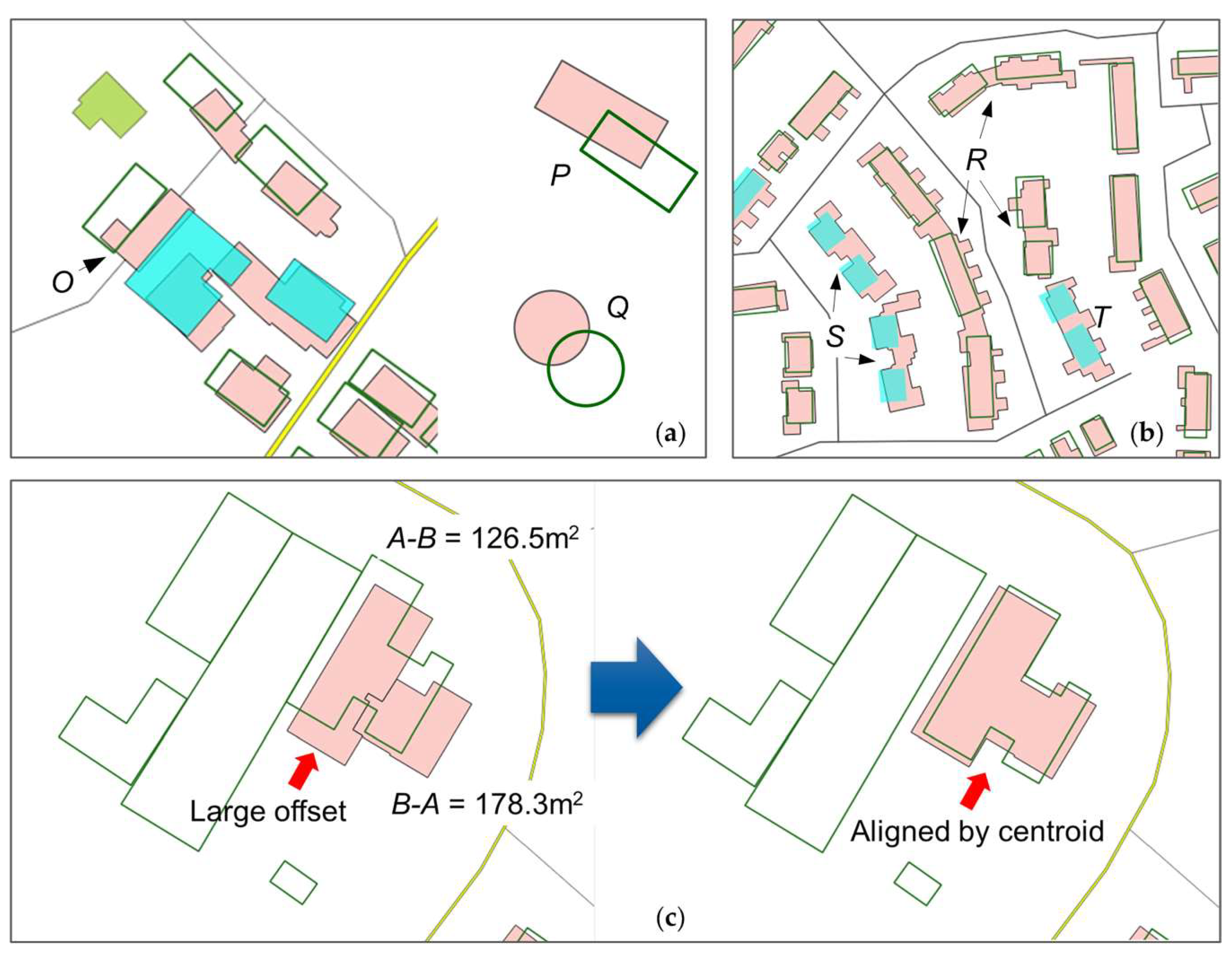
Set-based similarity: For any two overlapping polygons A and B, three basic sets can be distinguished: A-B, B-A, and A∩B (Figure 1). At the implementation level, A and B result in three non-overlapping polygons, some of which may contain multiple parts (Figure 1b). Basic geometric measures and advanced morphological analysis are performed on these parts.

(3)

Shape-based analysis [25] for measuring building similarity and characterizing the overall shape and difference parts.

Before presenting our rules, we first explain in greater detail some key factors that should be prepared for our change analysis. Because the many-to-many correspondence is not a good form for geometric analysis, we first converted the relation to a 1-to-1 relation by the following aggregation.

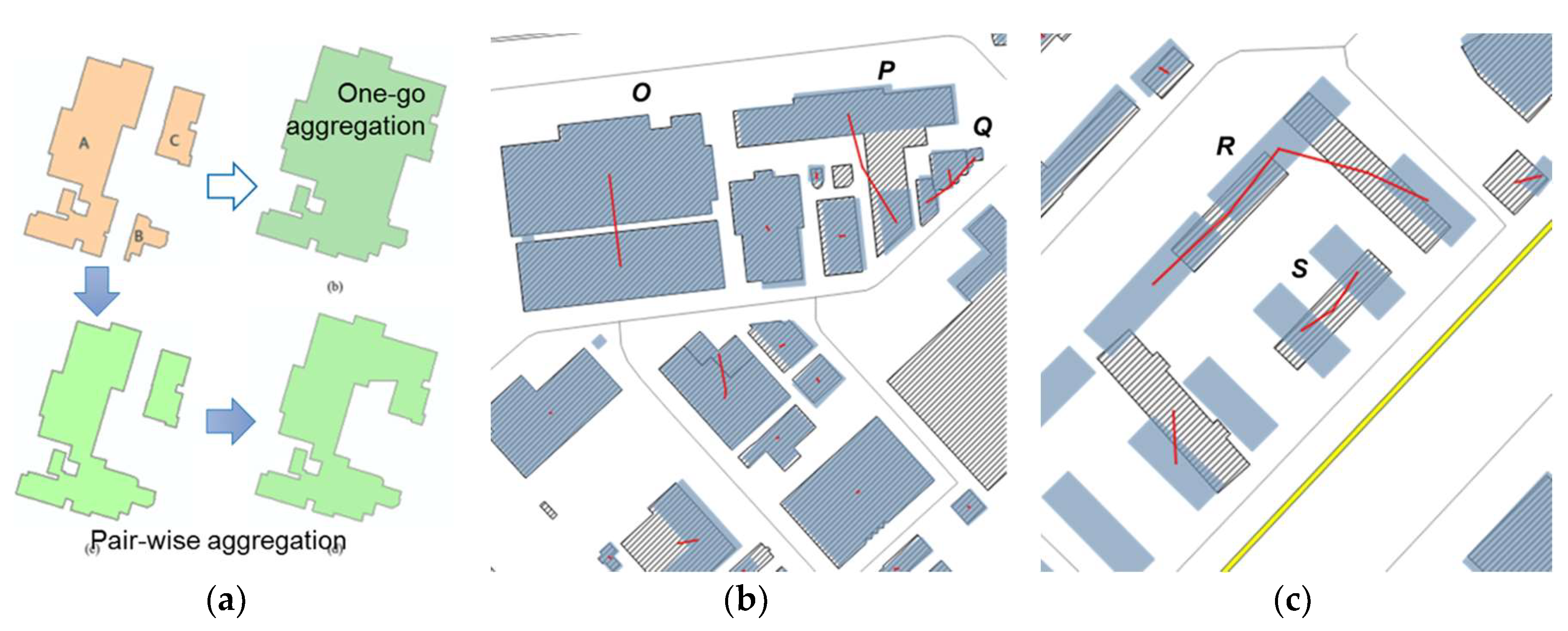
2.3.1. Aggregation with Minimum Cost for the Many-to-Many Correspondence

To perform change analysis for any m-to-n relationship, aggregation of the many objects in the relation is needed. Our aggregation was guided by the corresponding relation. For example, if {A₁, A₂, A₃} corresponds to {B₁, B₂}, then A₁, A₂, and A₃ should be aggregated to B₁ and B₂. To do so, we advocated a pair-wise aggregation (based on ArcGIS’s aggregation), which approximated the original outlines (Figure 3a) better than the one-go aggregation (available in ArcGIS). This is because each m-to-n relationship requires a different distance value for them to be aggregated. As a result, in the one-go aggregation, the value should be very large to ensure that all buildings included in the relation are aggregated. This could lead to an over-aggregated polygon (Figure 3a). Our pair-wise aggregation proceeds as follows: (1) calculating the distance between the m or n objects {o_i}; (2) aggregating building pairs with ArcGIS’s aggregation functionality in increasing order of distance until there are no more buildings to be aggregated; and (3) the aggregation is guarded with a post-evaluation: if too much empty space is enclosed by the aggregation, the buildings should have changed physically. The post-evaluation is performed using the following equation:

AggRatio ({o_i}) = (Area(Aggregate({o_i})) − Area({o_i}))/Area({o_i})

(2)

where {o_i} is either the m or n part in the m-to-n relation. If AggRatio ≥ T_{agg_ratio} (threshold for aggregation ratio), we stopped the aggregation as well as the subsequent shape analysis. The buildings in the relation were then marked ‘changed’. For example, P, R, and S in Figure 3 are situations where the aggregation could have enclosed too much empty space (e.g., T_{agg_ratio} = 0.2), indicating that they are situations where changes may occur. If the two buildings in P are aggregated, the shape comparison would lead to a conclusion that it had not changed. Finally, if the aggregation passes the post-evaluation, the m-to-n relation becomes a 1-to-1 relation and proceeds with the subsequent comparison.

2.3.2. Controlled Alignment of Corresponding Objects

To overcome the boundary mismatch issue (Section 2.2), objects should be aligned to ensure a more reliable shape-based change analysis. However, such an alignment should not be overdone, as offset is caused mainly by cartographic displacement, which is relatively large for small buildings. As a result, we mainly aligned small objects (<150 m²) with simple shapes (quantified in the following) by moving the objects toward each other’s centroid. For buildings with more complex shapes, such an alignment could introduce extra errors and is hence prohibited. For instance, building pairs in the center of Figure 4a,b are largely offset by just looking at their centroids. They are actually perfectly aligned with each other with expansion or contraction to the plans. As an exception, when A-B and B-A are comparable in size (i.e., Min(Area(A-B)/Area(B-A), Area(B-A)/Area(A-B)) ≥ 0.6), the two buildings are also aligned even for complex shapes (Figure 4c). This is because, in such situations, the discrepancy between the objects may be because of the positional deviation. The movement is used to alleviate this deviation and help the similarity comparison.

Offset is calculated as the distance between building centroids. To determine if a building in the corresponding relationship has a simple shape or not, we firstly simplified OSM buildings with a parameter suitable for TOP10NL, for example, we simplified intrusions and protrusions smaller than 5 m (Figure 4c), and then we calculated the convex hull of the simplified building. If the condition Area(simplified building)/Area(convex hull) ≥ 0.9 holds for both buildings in a corresponding relation, meaning that they are very similar to a rectangle, then we moved the two buildings so that their centroids aligned before the subsequent analysis. After the alignment, the difference parts A-B, B-A, and A∩B were re-generated.

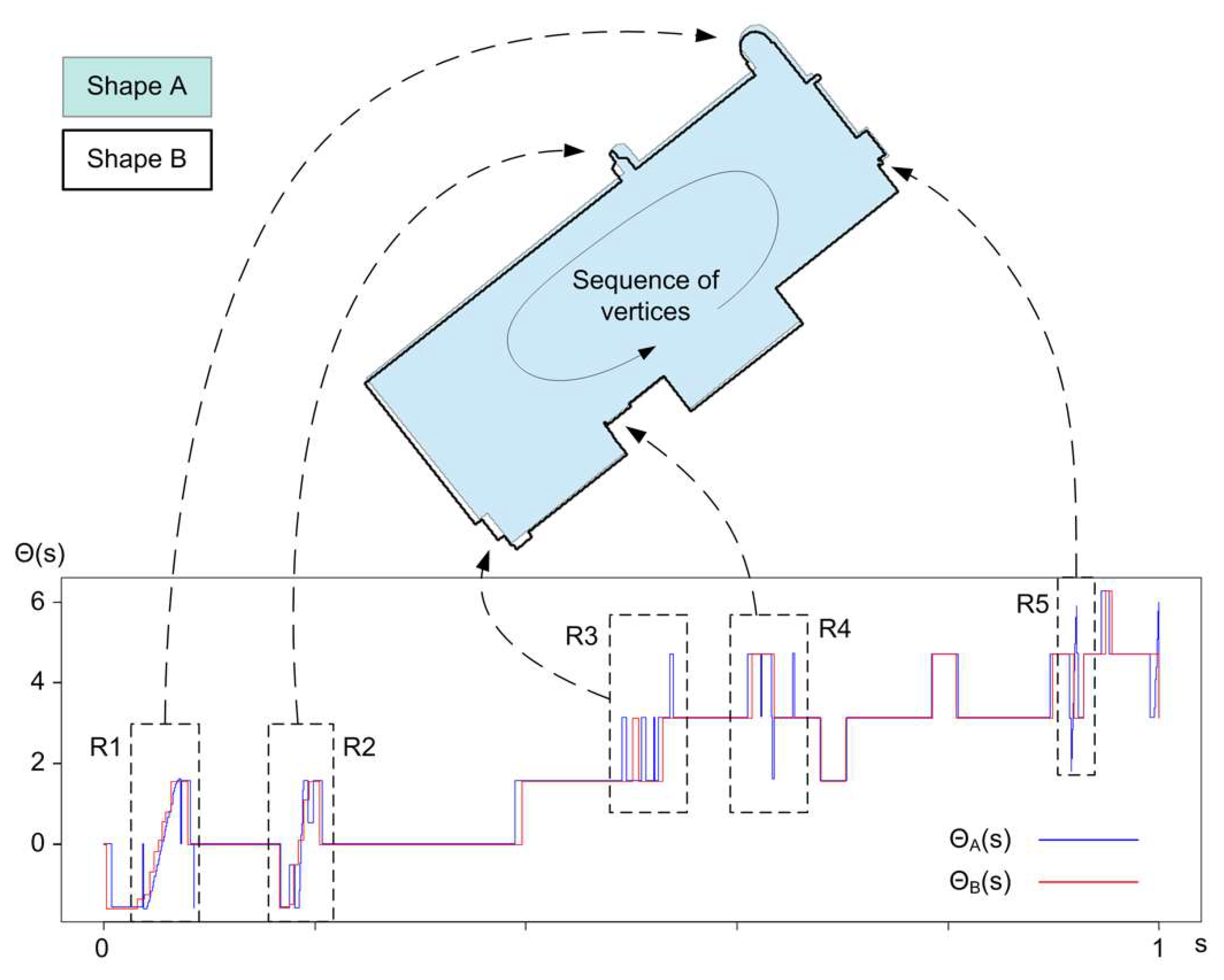
2.3.3. Global Shape Similarity Using Turning Function

Note that the above alignment cannot completely address the boundary mismatch problem for all situations, especially when the shapes are complex. In such cases, there is a reasonable chance that two similar shapes had shifted away from each other. The basic geometry-based change detection cannot properly handle this situation and indicates that changes occur for these situations (see, for example, Figure 1e).

The turning function is used here as a global shape similarity measure for building footprints and is given in the following equation [26]:

$$d^{A,B}\left(t,\theta \right)={\left(mi{n}_{\theta \in ℛ, t\in \left[0,1\right]}\underset{0}{\overset{1}{{\displaystyle \int }}}{\left({\Theta }_A\left(s+t\right)-{\Theta }_B\left(s\right)+\theta \right)}^{2}ds\right)}^{\frac{1}{2}}$$

(3)

For any polygon, the turning function Θ(s) describes the variation in the tangent-angle of its outline (in radians) in relation to the normalized arc-length s (e.g., Θ_A(s) and Θ_B(s) in Figure 5), where s ∈ [0, 1] is any point along the polygon outline and when s = {0,1}, it is situated on the start/end vertex. The distance d^A,B(t,θ) is the turning function similarity between A and B. For more details, please refer to previously published reports [26,27].

This shape similarity measure is used in here in two ways: to measure the general similarity of shapes, and to address the issue where very similar shapes are not aligned with each other. If the two similar shapes had a small turning function distance (e.g., d^A,B(t,θ) < 1.0) and were further comparable in size, we aligned them by their centroids for the subsequent analysis. This should be able to improve the change detection.

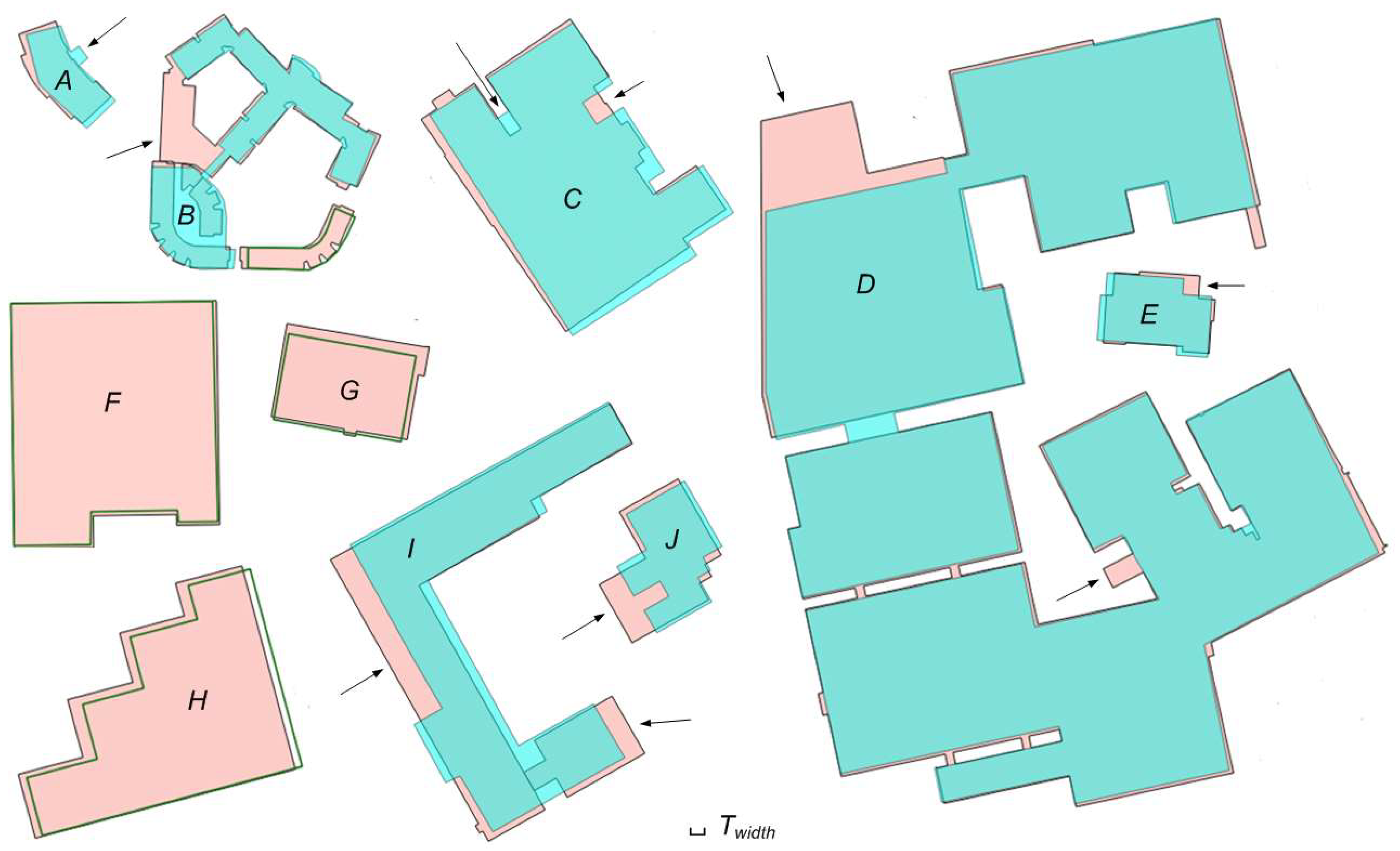
2.3.4. Morphological Analysis of Difference Parts

After merging m-to-n relations and performing necessary alignment, we overlapped two polygons A and B, which resulted in three parts (A-B, B-A, and A∩B). Analysis of these difference parts yielded insight into the change analysis. In particular, the morphology of the differences is important (e.g., Figure 1b). When the size of the difference is the same, the morphology of the difference significantly influenced our decisions about the results. For example, the green parts of Figure 6a,c,d are similar in size and all largely exceed the threshold for absolute size of the difference T_{size_diff_abs} (e.g., 100 m²) accounting for a change, but only the green part in Figure 6a is an obvious change (i.e., a small expansion). If we considered absolute size, all three cases should be regarded as ‘changed’; if we considered the relative size of the difference in relation to the entire building (i.e., Area(difference part)/Area(x), where x ∈ {A, B}), the situation in Figure 6a would be regarded as ‘unchanged’. What makes them different is whether the difference is fragmented into small pieces (Figure 6d) and how the parts are shaped and distributed (c.f. Figure 6a,c). For the individual house in Figure 6b, the expansion is not even up to T_{size_diff_abs}. To account for the fact that it changed, the threshold for the relative size of the difference (T_{size_diff_rel}) had to be used.

The above observations have two implications: (1) a fixed threshold is insufficient for identifying true changes, and distinguishing between small and large objects is useful in establishing our rules and parameters. Although more size classes may be proven even better, we wanted to keep the rules simple and more intuitive to better demonstrate our approach and the identified factors; (2) analysis of the morphology of the difference becomes important. We thus derived the following process in our morphologic analysis:

• For small buildings, absolute and relative size of the difference should be considered.
• For large buildings, absolute size of the difference is used as a first criterion, and if the size of the difference exceeds T_{size_diff_abs},
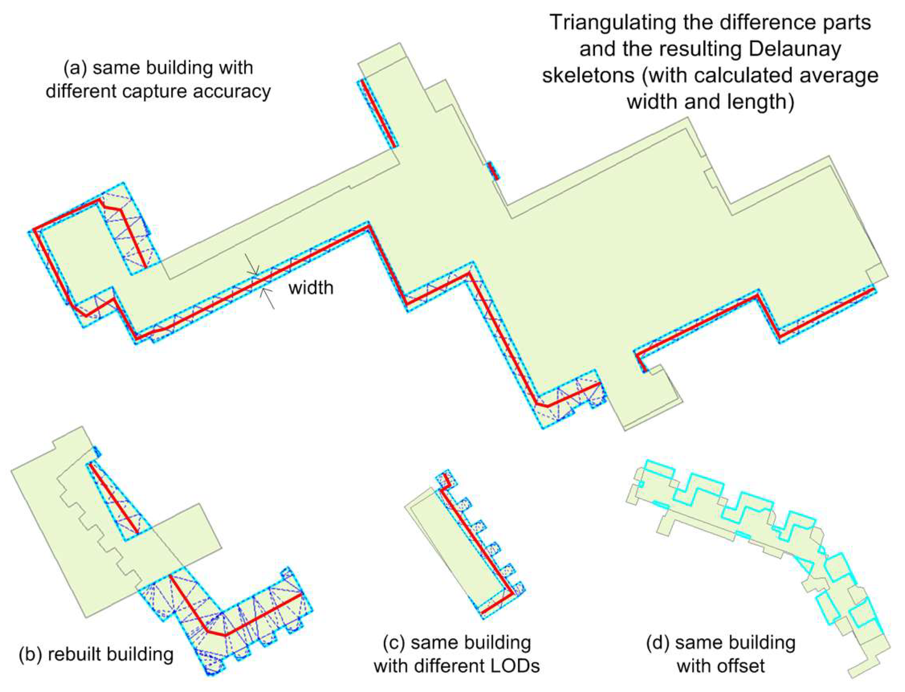
  • First check if the part can be segmented into multiple smaller pieces (Figure 7d). If any of them exceeds T_{size_diff_abs}, proceed with the analysis in sub-step b; if none of them is large enough, the building is regarded as unchanged;
  • For any significant part (or segmented piece), quantify their shape by examining if it is long and narrow, thin belt-shaped (not changed), or in a more compact form (changed).

Now, we present the details concerning the characterization of difference parts in sub-step b. For any difference part (whether original or segmented) that qualifies as a potential change (i.e., ≥T_{size_diff_abs}), we computed the constrained Delaunay triangulation (DT) on the polygon (dashed blue in Figure 7). The use of DT for morphologic analysis has a long history [28,29] and we used it to generate skeletons (i.e., center lines) for characterizing the morphology of difference parts. The basic idea was to track the triangles along the corridor of the polygon from end to end (red lines in Figure 7). This is a well-established technique, and the technical details of this technique have been previously published [30,31,32].

With skeletons and triangles, we were able to characterize the shape of the part. For example, the skeleton reflects the length (L_skeleton) along the stretch of the polygon (Figure 7a–c). With the triangles aligned along the skeleton, we calculated the average width (W_skeleton) [33]. The width of the difference is important for distinguishing changes from non-changes. If it is wider than the threshold (T_width), the difference part is regarded to be significant enough for a change. For example, Figure 6a and Figure 7b are regarded as changed. The elongation ratio as given below is also useful for characterizing if the difference is belt-shaped (if it is smaller than T_{elong_ratio}). We observed that if the difference part was a thin belt shape, for example, Figure 6c and Figure 7a,c, the object was also untouched.

ElongationRatio = W_skeleton/L_skeleton,

(4)

Note that in our approach, the above two thresholds T_width and T_{elong_ratio} are exposed as user parameters, so that in different applications, users can control the change detection results (see Section 4.1 for discussion).

2.3.5. Rules and Parameters

The above-mentioned rules, measures, and operations are organized in a directed acyclic graph (DAG) structure in our rule system (Figure 8). The algorithm starts from matching corresponding objects (Section 2.2), which results in different types of relations. The 1-to-0 and 0-to-1 relations indicate new and demolished buildings, respectively. The m-to-n relations are aggregated into 1-to-1 relations using the procedures in Section 2.3.1. All qualified 1-to-1 relations were aligned (Section 2.3.2.) before the rule-based change detection occurred. For small buildings in particular, we did not look at their turning function similarity (Section 2.3.3), because the measure is easily influenced by the discrepancies in LOD between OSM and our TOP10NL data and is hence not reliable. However, the morphology of difference parts (Section 2.3.4) was still used to leave out those small and belt-shaped parts from true changes (the last rules in Figure 8). Specifically, if the part was wide enough (e.g., W_skeleton ≥ 5 m), it was considered a changed part (e.g., expansion); if it was not wide enough but was large enough (e.g., the part was larger than Min(100 m²), 20% of the building) and in a compact form (e.g., ElongationRatio ≥ 0.2), it was also considered a change. The definitions of wide parts and belt-shape parts were controlled by T_width and T_{elong_ratio}, which are exposed as user parameters.

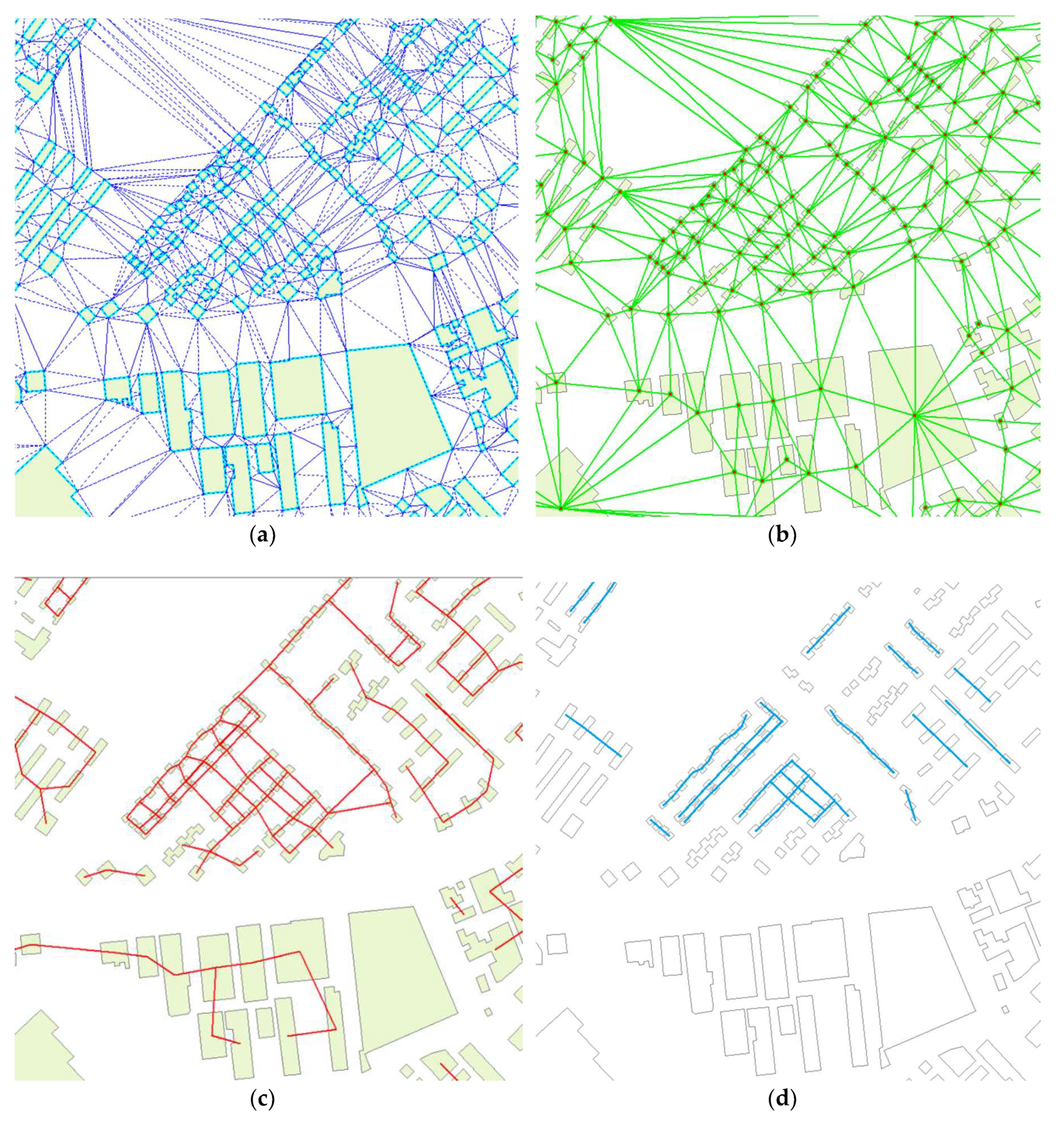
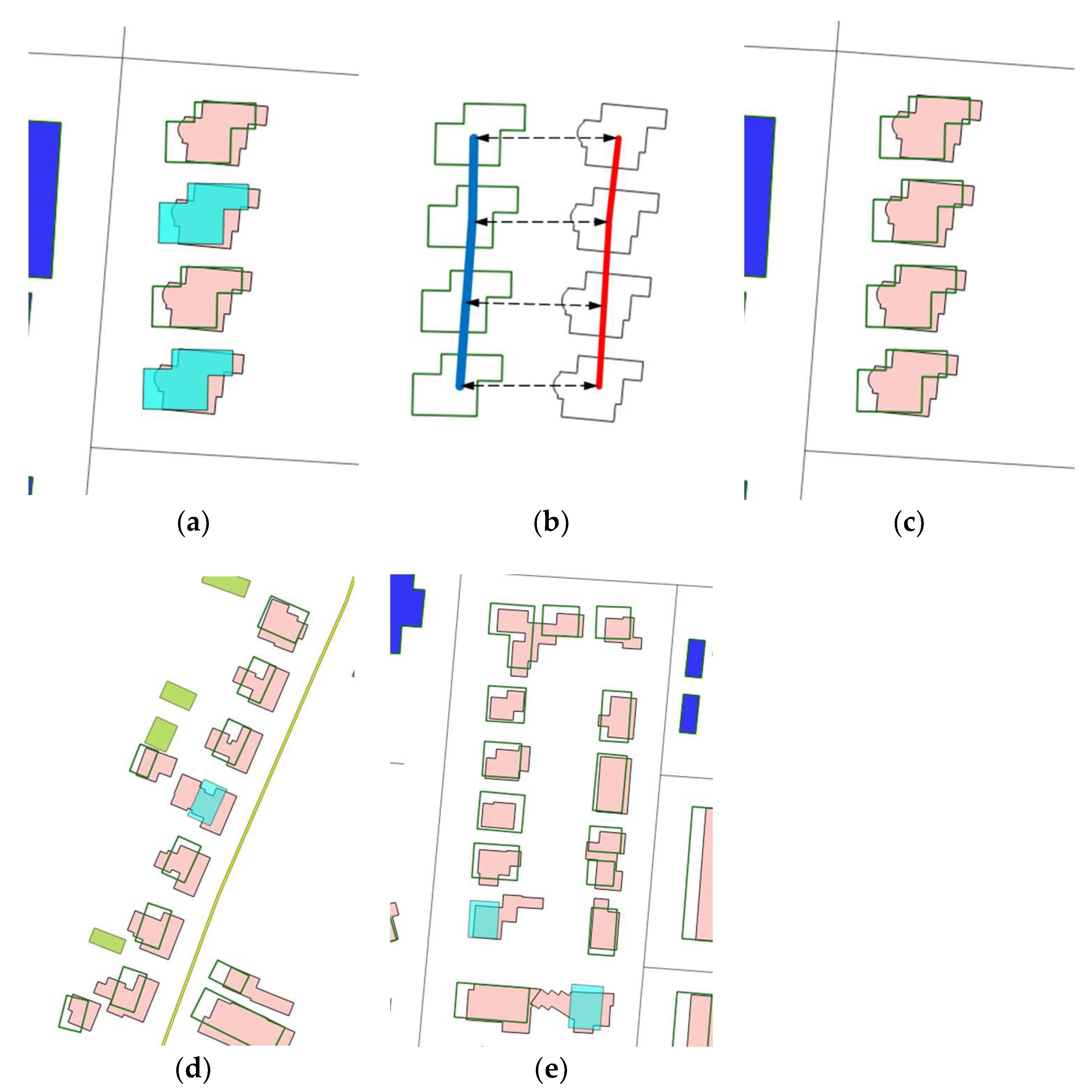
2.4. Correcting Detected Changes with Pattern and Contextual Information

As noted in Section 2 (Figure 1h), the detected changes are sensitive to small variations in size and position of the buildings. We observed that such sensitivity can be counteracted by viewing buildings in a group, where building patterns and alignments provide useful heuristics [34,35]. The underlying assumption is that buildings in certain alignments (e.g., grid-like and linear patterns) are less likely to be modified as an individual; replacement or rebuilding as a whole and addition/removal of buildings from the plan are more probable. This is because a significant alignment (e.g., a residential neighborhood) commonly indicates that its constituent buildings were designed, built, and managed as a whole. This heuristic is used in our approach to refine the inconsistent changes in such alignments.

An alignment is a homogeneous group of buildings that are evenly spaced and have similar forms, sizes, and regular layout. The steps in recognizing the alignments from building footprints are briefly outlined in the following section (for details, refers to Zhang et al. [35], Figure 9):

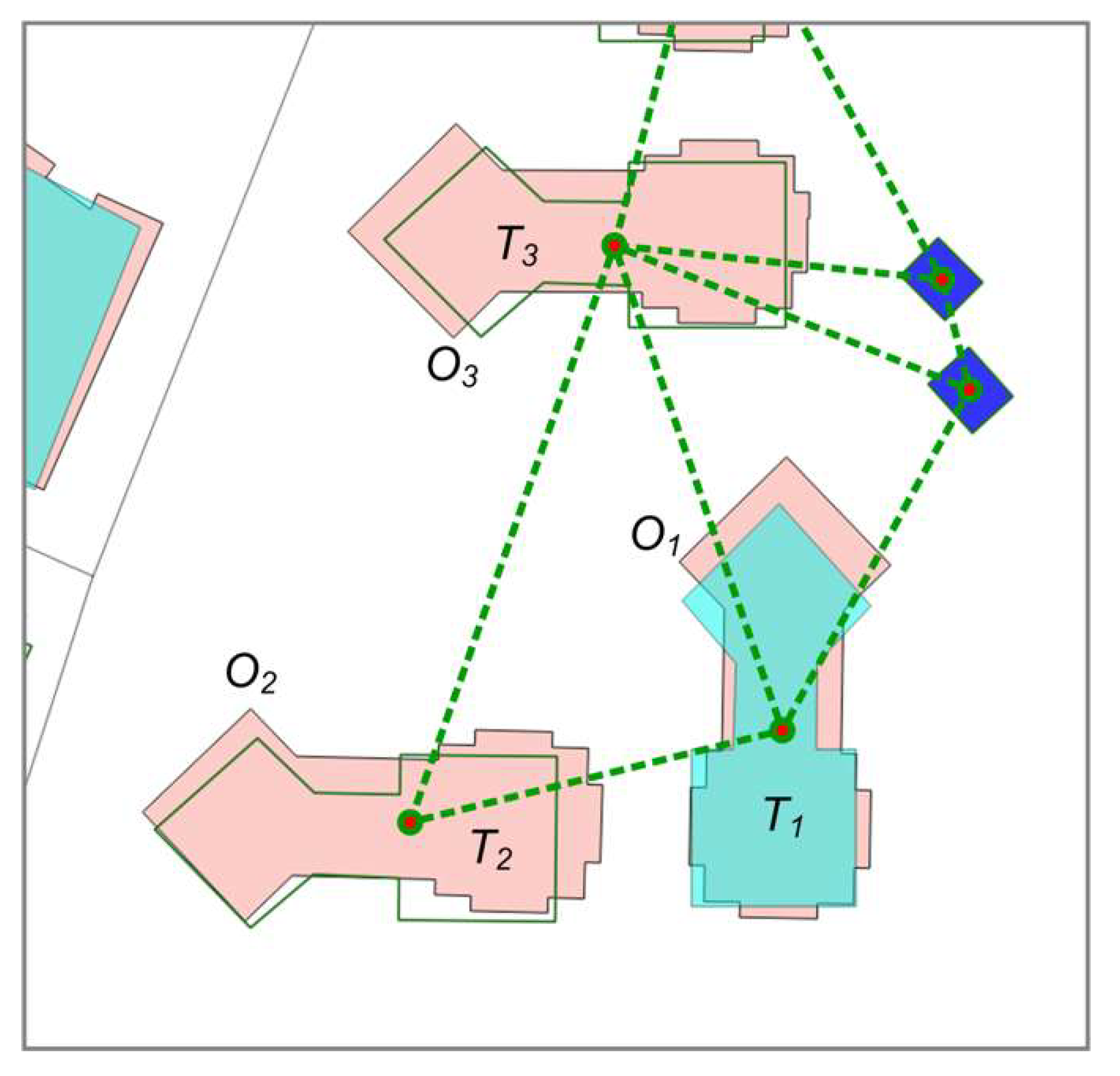
• Compute Delaunay triangulation (DT) on the data area.
• Derive the proximity graph of building footprints, ProxG〈V, E〉, where V is the set of buildings and E is the set of building pairs connected by at least a triangle.
• Prune any edge in ProxG if its two connecting buildings are very different in size, shape, and orientation.
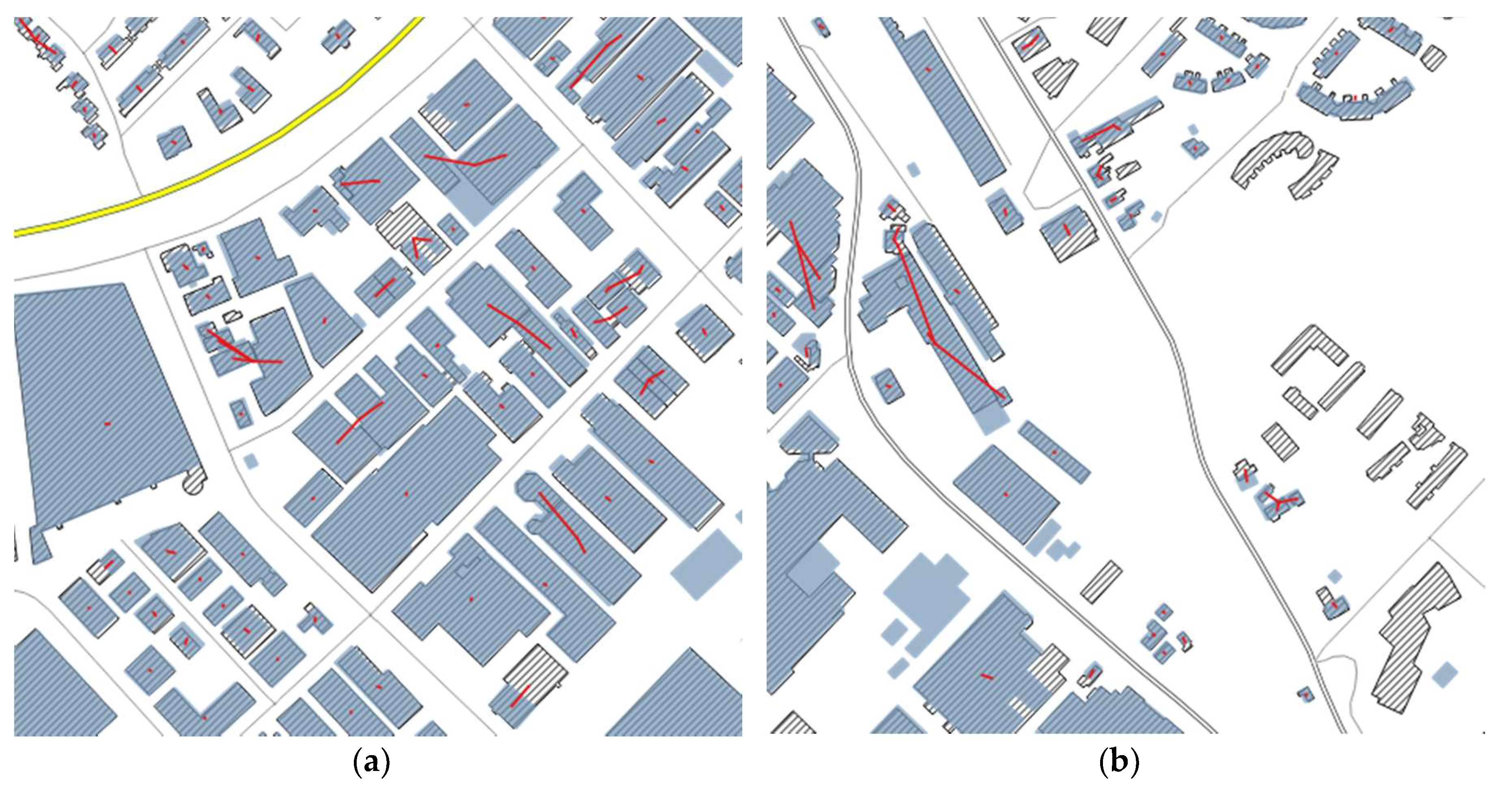
• Trace alignments in the pruned ProxG following the criteria in Zhang et al. [35] and characterized by their homogeneity value (i.e., significance).

For this type of knowledge to be useful, we needed to know if the pattern/alignment was maintained in its entirety in the two datasets. If the alignment was maintained in both datasets, the buildings in the group were considered unchanged with a higher probability. To be on the safe side, we only re-assigned the detected changes that slightly exceeded the threshold (i.e., within a small tolerance) in a kept alignment to be unchanged (we call this inconsistency correction).

To implement this idea, significant alignments were recognized for both current and to-be-updated data. Then, corresponding alignments in the two data sets were matched using simple positional and geometric similarity measures [36]. Finally, if we found all buildings in the two alignments also corresponded to each other, we considered the two alignments to be well maintained and applied the above inconsistency correction procedure (see Section 3.2.3 for a demonstration).

3. Experiment Design and Results

Our change detection methodology, including the measures (e.g., turning function), building simplification, DT-based morphology analysis, and building pattern recognition, were implemented with ArcObject and partly in C++.

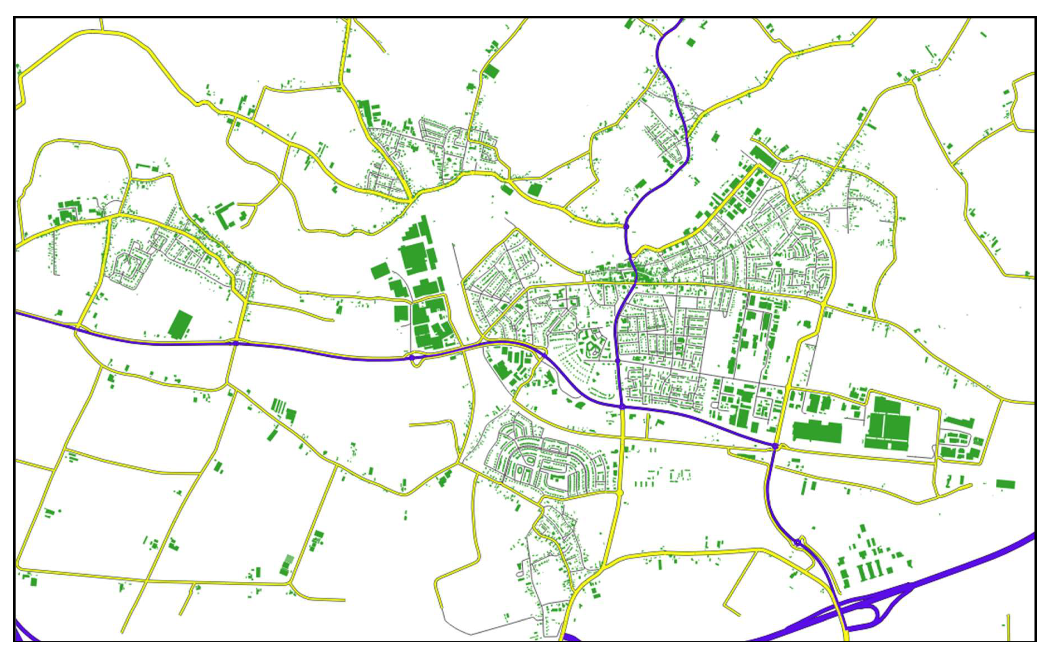
3.1. Data Description and Evaluation Methods

Our datasets consisted of the more current OSM data (5420 buildings) and the to-be-updated TOP10NL data (4606 buildings) in Geldermalsen, NL. Figure 10 shows a sample area of our test datasets, which is populated with diverse land-use characteristics. First, OSM data were projected with ‘Amersfoort/RD New’ to minimize its offset (positional discrepancy) to TOP10NL. We then measured the offset between the two for the 1-to-1 relation, which was generally below ~9 m (with a median of 3.38 m). This confirms that the boundary mismatch issue is widespread. A measure of building size showed that about 60% of buildings were smaller than 150 m², which is just about the size of an individual house. Thus, we used it as a threshold to distinguish small from large buildings.

Reference values for change detection were labeled by human experts. We measured true positives (tp; when our algorithm agreed with experts on a change; here, change includes ‘New’, ‘Changed’, and ‘Removal’ in Figure 11), false positives (fp; algorithm finds a change but experts do not agree), true negatives (tn; algorithm agree with experts on a non-change), and false negatives (fn; algorithm finds a non-change but experts do not agree). Precision = tp/(tp + fp), recall = tp/(tp + fn), accuracy = (tp + tn)/(tp + fp + tn + fn) and Cohen’s kappa coefficient (k) were used to evaluate the performance of our approach. To obtain further insight into the effectiveness of our approach, especially the chosen rules, we ran our approach in different versions (with and without some of the rules and components).

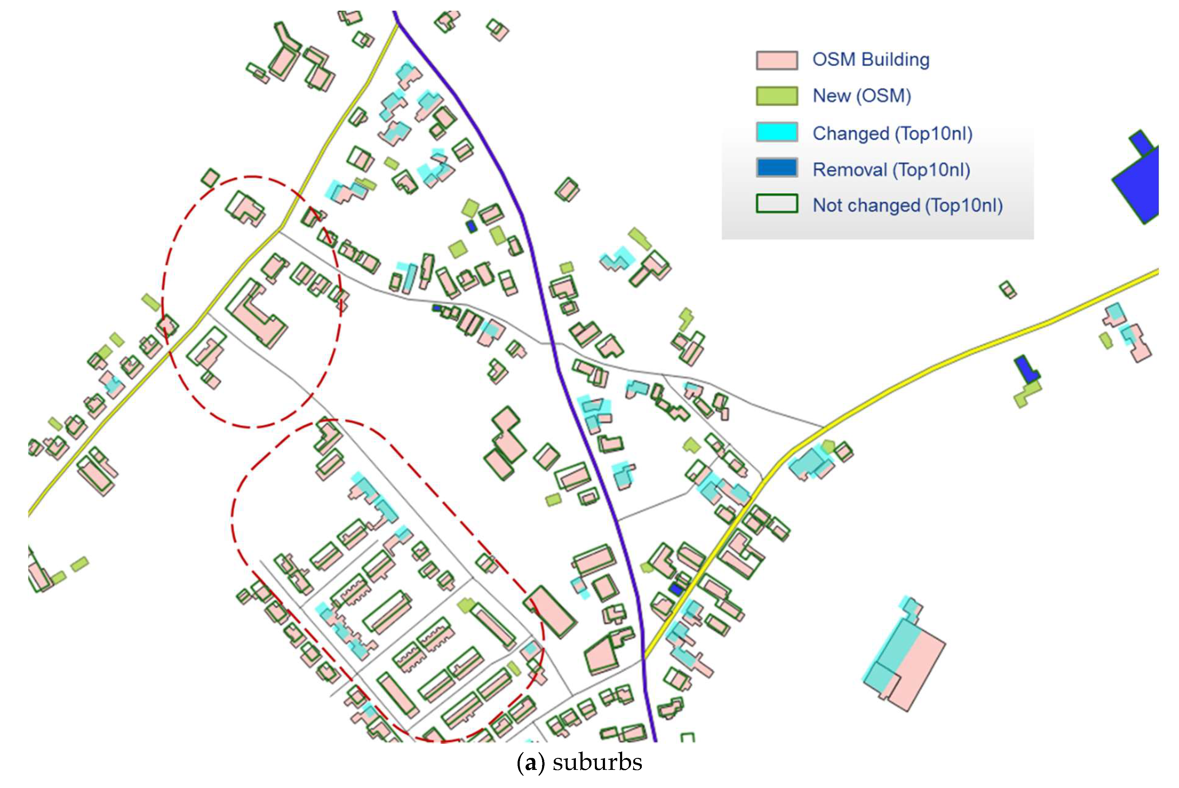
3.2. Detected Changes

3.2.1. General Results

In general, our approach performed well in identifying the changes (Figure 11), though there were some imperfections. We noticed that in the areas highlighted in Figure 11a, the offset and boundary mismatch, caused much difficulty in change detection. However, our approach produced a satisfactory result owing to the use of the controlled alignment technique (Section 2.3.2). We noticed that uncertainty existed in some situations where experts were not sure of their labelling (Section 4.1 for further discussion). In Figure 11b,c, many detected changes are large buildings modified in part (e.g., expanded or contracted). This is attributed to the use of morphology analysis (Section 2.3.3). The general performance is measured in

Table 1. The performance of our change detection algorithm in three versions (all values range from 0 to 1 and a higher value indicates a higher level of satisfaction).

Method	precision	recall	accuracy	k
Basic 1	0.55	0.76	0.77	0.47
Advanced 2	0.82	0.87	0.90	0.77
Advanced + Pattern 3	0.87	0.87	0.92	0.81

¹ basic geometric analysis without controlled alignment and morphology analysis (the one produced the results in Figure 1); ² with controlled alignment and morphology analysis; ³ corrected by the pattern constraint.

(i.e., ‘Advanced’).

3.2.2. Effectiveness of the Chosen Rules and Parameters

First, we used CommonAreaRato ≥ 15% for object matching, which was relaxed from the value of 30% that was previously used [5,24] (Section 2.2). Without this relaxation, pairs O, P, and Q in Figure 12a could not be matched because of the large offset. Because O, P, and Q are simple shapes, they were aligned by our algorithm to reduce their apparent difference and were classified as unchanged (true negatives). With the basic method (based solely on sizes of difference parts) in Table 1, however, they were classified as changed (false positives). As the positional discrepancy was pervasive and could not be corrected by geo-referencing, errors resulted from the basic geometric analysis. The basic method reduced the number of false negatives (high recall) at the risk of including more false positives (low precision).

The threshold for aggregation ratio (T_{agg_ratio} = 0.2) that was used to evaluate whether we could turn an m-to-n relation into a 1-to-1 relation (Section 2.3.1) also had an effect on the detected results. For instance, R in Figure 12b points to situations where the post-evaluation was passed and the subsequent analysis (e.g., morphology analysis) proceeded. S and T failed to pass the post-evaluation and were directly identified as changed (see our rules in Figure 8). By adjusting T_{agg_ratio}, we obtained different results. However, S, R, and T in Figure 12b are highly ambiguous and we did not have a golden standard to judge which result was more correct (see Section 4.1).

Note that the parameter values were empirically determined so they might have fitting or overfitting problems. To generalize our approach to other datasets, machine learning could be an option (see Section 4.4).

Figure 12c demonstrates how a large offset can be counteracted by controlled alignment, and hence correct results were produced. First, our algorithm merged the two OSM buildings in this 2-to-1 relationship. Then, it concluded that A-B and B-A are comparable in size, indicating a possible case of similar shapes shifted away from each other. Finally, our algorithm tried to align the TOP10NL building to its OSM counterpart, and carried out the subsequent set-based, shape, and morphology analysis, which predicted that the situation had not changed. This exemplifies the importance of controlled alignment in handling the boundary mismatch problem in certain situations.

Now, we look into some details of the morphology analysis (Section 2.3.4) in Figure 13. Here, the difference parts in A, C, and E are the smallest, even smaller than those of F, G, and H. Our morphology analysis was able to identify that F, G, and H were unchanged, as the skeleton width of their parts was less than T_width (e.g., 5 m in the presented results) and the elongation ratio was very low. Many long and thin-belt parts in other buildings in Figure 13 were identified using the same process. This was useful for further identifying where the expansion or contraction occurred (e.g., arrows in Figure 13).

The advanced method (Table 1) that considered the above factors performed remarkably better than the basic method. A closer look at the process revealed that about 63% of the buildings were temporarily aligned in the advanced version, which is a major improvement in performance.

3.2.3. Corrections Guided by Building Patterns

As mentioned in Section 2.2, small variations in geometry can lead to inconsistent results if viewed in context. Here, we evaluate how contextual knowledge, such as building alignments (Section 2.4), could help improve our change detection.

In total, we recognized 126 alignments that were present in both OSM and TOP10NL, among which we only selected significant alignments with homogeneity values ≤1.5 [35]. In these alignments, we looked for buildings that were assigned as ‘changed’ by the advanced method. If these buildings only slightly exceeded the criteria, for example, (measured value − threshold)/threshold ≤ 10%, they were re-assigned by this inconsistency correction procedure as ‘unchanged’. For example, the two light blue buildings in Figure 14a were classified as ‘changed’ because their parts were large compact shapes (i.e., larger than 20% of the original building) by exceeding the threshold slightly by less than 1%. The other two (white) in the alignment were below this threshold, though their parts were also compact (i.e., ElongationRatio > 0.2). Therefore, the two blue buildings were corrected to be ‘unchanged’ (Figure 14a,c). We cannot be sure about this correction if the buildings are not present in a special pattern.

On the other hand, the blue buildings in alignment in Figure 14d,e were not corrected in this procedure because their parts significantly exceeded the criteria. Consequently, they stayed as ‘changed’. Although experts labelled the two cases as ‘unchanged’ (they said that the differences were the result of different specifications), they agreed that the situations are highly uncertain, and hence their reference value should be taken with care. Thus, we tried not to overanalyze this aspect.

Finally, our algorithm corrected 94 cases with this conservative treatment, substantially improving performance (Table 1). Because such a correction only reduces false negatives and increases true negatives, it does not improve the recall rate.

To summarize, we experimentally confirmed that the controlled alignment, morphology analysis, and pattern constraint are three important components in this challenging problem. Given the ambiguities involved, we found that the final results are quite satisfactory.

4. Discussion

4.1. Uncertainty and User Parameters

We showed that to determine whether an object is changed or not is highly ambiguous even for datasets of a similar scale (e.g., OSM and TOP10NL). The experts also confirmed such uncertainty in the labeling of changes. For example, S, R, and T in Figure 12 and A, C, E, I, and J in Figure 13 were classified differently by different experts. Recording this uncertainty during the labeling should be insightful for evaluating our approach in the future. Noticeably, the uncertainty was partly because OSM and TOP10NL datasets use different specifications in this particular region (Geldermalsen, NL). We did not explicitly handle this issue, as some further assumptions were required that may not be applicable elsewhere. From a different perspective, it would also be useful to inform stakeholders of the uncertainty in the detected changes for better decisions.

Nevertheless, the question is sometimes more about whether a change is significant enough for a certain purpose, rather than if it is a change. To this end, the user parameters that determined the width of a significant part (T_width) and its elongation ratio (T_{elong_ratio}) are useful. For example, we set T_width = 5 m because in our TOP10NL data, protrusions or intrusions with a width less than five meters were simplified when the data were registered in the database. For instance, by setting T_width = 10 m, A, C, E, and I in Figure 13 became ‘unchanged’ to a different application. This provides a flexible method for users to decide which changes are meaningful to them for their own purposes.

4.2. Effect of Scales on Change Detection

For datasets produced by the same data provider, boundary mismatch may not be a problem. It is thus possible to detect changes within an acceptable rate even when there is substantial discrepancy in scale [17]. However, sometimes boundary mismatch still exists for the data within the same organization, where finding corresponding objects across multiple scales becomes challenging [23]. For datasets maintained by different organizations (e.g., OSM and professional data), change detection becomes challenging because of differences in data capture, specification, and LOD among the organizations. The task as presented in this paper is already challenging enough given their similar scales in data capture. Zhang et al. [19] showed that as the difference in scale increases, reliable change detection tends to be increasingly difficult (if not impossible). As a result, we recommend that, without prior knowledge, change detection should be applied only for datasets that have scales as close to each other as possible. Furthermore, change detection is better performed at larger scales. This is because different organizations tend to adopt different protocols in generalizing their datasets at smaller scales, leading to false positive discrepancies.

4.3. Potential Use of Contextual Information

Currently, we used knowledge of building alignments to constrain our detection results. In essence, when buildings are located in an alignment they are in a functional context. We showed that such contextual information improved our detection accuracy (Table 1). In our experiment, we found that the proximity relationship can be used to improve inconsistent results.

As illustrated in Figure 15, T₁ was classified as ‘changed’ (a false positive). When compared with its surrounding cases, this inconsistency was the result of small geometric variations. First, the turning function value between O₁ and T₁ was 1.2, so they were not aligned to reduce the apparent difference. Then, it could not be corrected by the alignment constraint as the buildings were not in any alignment. Here, we propose the following idea: if a situation is very similar to its neighbors, the result among the similar neighbors can be cross-validated for inconsistency correction. Specifically, the turning function value among T₁, T₂, and T₃ was about 0.012, and that between O₁, O₂, and O₃ was about 0.19, which means that situations 〈O₁, T₁〉, 〈O₂, T₂〉, and 〈O₃, T₃〉 were nearly identical. Then, along a similar line of thought as in Section 3.2.3, T₁ can be corrected and re-assigned as ‘unchanged’. This shows another way where contextual information can play a role. We think that greater usage of contextual information can be identified in change detection when presented with more diverse data.

4.4. Fit into Machine Learning?

Without doubt, the change detection can be formulated as a classification problem using C4.5, naïve Bayes, or support vector machine (SVM) models. However, it is not currently clear if the results from machine learning can be comparable to our results. The main reason is that some of the prominent factors used in our approach are not readily accessible in the form of features in a classification problem. For example, morphological analysis of difference parts can lead to a non-fixed number of descriptors for different objects, which causes difficulties in a standard machine learning framework. Hence, by translating our approach into a machine learning model, we have to simplify or even discard some of the analysis shown to be critical in change detection.

Our approach is a mixture of rules and operations (e.g., displacement, simplification, shape analysis). The latter is applied on-demand for certain situations during change detection. For example, whether buildings in Figure 12c need to be aligned or not depends on whether or not the difference parts are comparable in size. Currently, we used a parameter value of 0.6. If this value was learned from data, it would be hard to predetermine which objects should be aligned from the outset. This is critical because the movement of buildings generates an updated set of features, that is, shape and size descriptors of the difference parts, as in Figure 12c. It will be challenging to mix rules and operations in machine learning correctly, as the algorithm tries different parameter values, and each turn generates dynamically new features for the training in this round.

Additionally, because parameters are learned from training samples in machine learning, not much room is left for user-specified parameters. The prediction of whether a building is changed or not can be determined, but the details concerning a change are not provided. In our approach, however, the dimensions (width, length, and elongation ratio) of the parts are left to the user to fine-tune the results, as in Section 4.1. However, this can be ill-fitted for machine learning. To achieve similar effects, different versions of training samples could be prepared for different user-defined parameter values, leading to many learned models (one model for each parameter value). This can be frustrating for both training and predicting.

Note that the main objective of this paper was to identify the factors crucial for change detection and propose computational methods for their measurement. Hence, we tried to keep our rules as clear and compact as possible. A more complicated rule system would definitely yield better results, but that is not the point for a manually crafted rule set. With machine learning, we obtain more complicated models (e.g., rule tree), optimized parameter values, and probabilistic prediction power (with certain classifiers). In a next step, we will determine how the important factors identified here can be fitted into a machine learning framework.

5. Conclusions

In this paper, we identified several measurable factors for change analysis that can properly handle boundary mismatch, LOD differences, generalization, and non-systematic offset that exist between datasets and are commonly encountered in current database update scenarios. In our case, OpenStreetMap was used to update professional data, so changes were derived by comparing the two. Specifically, data matching, aggregation of the many-to-many correspondence, controlled alignment, and morphology analysis of difference parts were identified as important factors and integrated for our change detection. The rules and operations were parameterized and organized in a directed acyclic graph structure, which is different from a typical decision tree.

The results showed that our approach based on these factors is much more powerful (accuracy = 0.90, kappa = 0.77) than a basic geometric method (0.77, 0.47, respectively). The main reason for this finding is that the pervasive non-systematic offset (median: 3.38 m, max.: ~9 m) between OSM and our data was largely handled by the controlled alignment in our approach. By further using knowledge of building patterns, many inconsistent results were corrected, yielding even better performance (0.92, 0.81, respectively). Considering the uncertainty involved, we are quite satisfied with this result.

We found further that distinguishing between small and large objects and setting different rules for them was a useful strategy in change detection. For heterogeneous data, shape discrepancies were common for small objects due to different levels of generalization used. As a result, it is less meaningful to compute shape similarity for small objects. In the future, we will look at how the important factors can be transferred into a machine learning framework to better handle the uncertainty during change detection, which could further facilitate applications in urban studies, geoinformatics, and real estate practices.

References

1. Haklay, M. How good is volunteered geographical information? A comparative study of OpenStreetMap and ordnance survey datasets. Environ. Plan. B Plan. Des. 2010, 37, 682–703. [Google Scholar] [CrossRef]
2. Neis, P.; Zipf, A. Analyzing the contributor activity of a volunteered geographic information project—The case of OpenStreetMap. ISPRS Int. J. Geo-Inf. 2012, 1, 146–165. [Google Scholar] [CrossRef]
3. Stoter, J.E.; van Smaalen, J.; Bakker, N.; Hardy, P. Specifying map requirements for automated generalisation of topographic data. Cartogr. J. 2009, 46, 214–227. [Google Scholar] [CrossRef]
4. Zielstra, D.; Zipf, A. A Comparative Study of Proprietary Geodata and Volunteered Geographic Information for Germany. In Proceedings of the 13th AGILE International Conference on Geographic Information Science, Guimarães, Portugal, 10–14 May 2010. [Google Scholar]
5. Fan, H.; Zipf, A.; Fu, Q.; Neis, P. Quality assessment for building footprints data on OpenStreetMap. Int. J. Geogr. Inf. Sci. 2014, 28, 700–719. [Google Scholar] [CrossRef]
6. Touya, G.; Brando-Escobar, C. Detecting level-of-detail inconsistencies in volunteered geographic information data sets. Cartogr. Int. J. Geogr. Inmation Geovis. 2013, 48, 134–143. [Google Scholar] [CrossRef]
7. Olteanu-Raimond, A.-M.; Hart, G.; Foody, G.M.; Touya, G.; Kellenberger, T.; Demetriou, D. The scale of VGI in map production: A perspective on European national mapping agencies. Trans. GIS 2016, 21, 74–90. [Google Scholar] [CrossRef]
8. Matikainen, L.; Hyyppä, J.; Ahokas, E.; Markelin, L.; Kaartinen, H. Automatic detection of buildings and changes in buildings for updating of maps. Remote Sens. 2010, 2, 1217–1248. [Google Scholar] [CrossRef]
9. Tian, J.; Cui, S.; Reinartz, P. Building change detection based on satellite stereo imagery and digital surface models. IEEE Trans. Geosci. Remote. Sens. 2014, 52, 406–417. [Google Scholar] [CrossRef] [Green Version]
10. Bouziani, M.; Goïta, K.; He, D.-C. Automatic change detection of buildings in urban environment from very high spatial resolution images using existing geodatabase and prior knowledge. ISPRS J. Photogramm. Remote Sens. 2010, 65, 143–153. [Google Scholar] [CrossRef]
11. Ye, S.; Chen, D.; Yu, J. A targeted change-detection procedure by combining change vector analysis and post-classification approach. ISPRS J. Photogramm. Remote Sens. 2016, 114, 115–124. [Google Scholar] [CrossRef]
12. Wijngaarden, F.; Putten, J.; Oosterom, P.; Uitermark, H. Map Integration—Update Propagation in a Multi-source Environment. In Proceedings of the 5th ACM International Workshop on Advances in Geographic Information Systems, Las Vegas, NV, USA, 10–14 November 1997; pp. 71–76. [Google Scholar]
13. Mas, J.F. Change estimates by map comparison: A method to reduce erroneous changes due to positional error. Trans. GIS 2005, 9, 619–629. [Google Scholar] [CrossRef]
14. Kuo, C.; Hong, J. Interoperable cross-domain semantic and geospatial framework for automatic change detection. Comput. Geosci. 2016, 86, 109–119. [Google Scholar] [CrossRef]
15. Qi, H.; Li, Z.; Chen, J. Automated change detection for updating settlements at smaller-scale maps from updated larger-scale maps. J. Spat. Sci. 2010, 55, 133–146. [Google Scholar] [CrossRef]
16. Zhang, X.; Guo, T.; Huang, J.; Xin, Q. Propagating updates of residential areas in multi-representation databases using constrained Delaunay triangulations. ISPRS Int. J. Geo-Inf. 2016, 5, 80. [Google Scholar] [CrossRef]
17. Yang, M.; Ai, T.; Yan, X.; Chen, Y.; Zhang, X. A map-algebra-based method for automatic change detection and spatial data updating across multiple scales. Trans. GIS 2018, 22, 435–454. [Google Scholar] [CrossRef]
18. Brychtová, A.; Çöltekin, A.; Paszto, V. Do the visual complexity algorithms match the generalization process in geographical displays? In Proceedings of the XXIII ISPRS Congress, Commission II, Prague, Czech Republic, 12–19 July 2016; pp. 375–378. [Google Scholar]
19. Zhang, X.; Yin, W.; Yang, M.; Ai, T.; Stoter, J. Updating authoritative spatial data from timely sources: A multiple representation approach. Int. J. Appl. Earth Obs. Geoinf. 2018, 72, 42–56. [Google Scholar] [CrossRef]
20. Xie, X.; Wong, K.; Aghajan, H.; Veelaert, P.; Philips, W. Road network inference through multiple track alignment. Transp. Res. Part C 2016, 72, 93–108. [Google Scholar] [CrossRef]
21. Liu, C.; Xiong, L.; Hu, X.; Shan, J. A progressive buffering method for road map update using OpenStreetMap data. ISPRS Int. J. Geo-Inf. 2015, 4, 1246–1264. [Google Scholar] [CrossRef]
22. Touya, G.; Reimer, A. Inferring the scale of OpenStreetMap features. In OpenStreetMap in GIScience: Experiences, Research, Applications; Jokar Arsanjani, J., Zipf, A., Mooney, P., Helbich, M., Eds.; Springer: Berlin, Germany, 2014; pp. 81–99. [Google Scholar]
23. Zhang, X.; Ai, T.; Stoter, J.; Zhao, X. Data matching of building polygons at multiple map scales improved by contextual information and relaxation. ISPRS J. Photogramm. Remote Sens. 2014, 92, 147–163. [Google Scholar] [CrossRef]
24. Rutzinger, M.; Rottensteiner, F.; Pfeifer, N. A comparison of evaluation techniques for building extraction from airborne laser scanning. IEEE J. Sel. Top. Appl. Earth Obs. Remote Sens. 2009, 2, 11–20. [Google Scholar] [CrossRef]
25. Pászto, V.; Brychtová, A.; Marek, L. On shape metrics in cartographic generalization: A case study of the building footprint geometry. In Modern Trends in Cartography; Brus, J., Vondrakova, A., Vozenilek, V., Eds.; Springer: Berlin, Heidelberg, 2014; pp. 397–407. [Google Scholar]
26. Arkin, E.M.; Chew, L.P.; Huttenlocher, D.P.; Kedem, K.; Mitchell, J.S. An efficiently computable metric for comparing polygonal shapes. IEEE Trans. Pattern Anal. Mach. Intell. 1991, 13, 209–216. [Google Scholar] [CrossRef] [Green Version]
27. Yan, X.; Ai, T.; Zhang, X. Template matching and simplification method for building features based on shape cognition. ISPRS Int. J. Geo-Inf. 2017, 6, 250. [Google Scholar] [CrossRef]
28. Jones, C.B.; Bundy, G.L.; Ware, J.M. Map generalization with a triangulated data structure. Cartogr. Geogr. Inf. Sci. 1995, 22, 317–331. [Google Scholar] [CrossRef]
29. Ai, T.; Guo, R.; Liu, Y. A binary tree representation of curve hierarchical structure based on Gestalt principles. In Proceedings of the 9th international symposium on Spatial Data Handling, Beijing, China, 10–12 August 2000; pp. 2a30–2a43. [Google Scholar]
30. Haunert, J.-H.; Sester, M. Area collapse and road centerlines based on straight skeletons. Geoinformatica 2007, 12, 169–191. [Google Scholar] [CrossRef]
31. Zhang, X.; Ai, T.; Stoter, J. The evaluation of spatial distribution density in map generalization. In Proceedings of the XXI ISPRS Congress, Beijing, China, 3–11 July 2008; Volume XXXVII, Part B2. pp. 181–187. [Google Scholar]
32. Ai, T.; Ke, S.; Yang, M.; Li, J. Envelope generation and simplification of polylines using Delaunay triangulation. Int. J. Geogr. Inf. Sci. 2016, 31, 297–319. [Google Scholar] [CrossRef]
33. Ai, T.; Zhang, X.; Zhou, Q.; Yang, M. A vector field model to handle the displacement of multiple conflicts in building generalization. Int. J. Geogr. Inf. Sci. 2015, 29, 1310–1331. [Google Scholar] [CrossRef]
34. Anders, K.H. Grid typification. In Progress in Spatial Data Handling; Riedl, A., Kainz, W., Elmes, G.A., Eds.; Springer: Berlin, Heidelberg, 2006; pp. 633–642. [Google Scholar]
35. Zhang, X.; Ai, T.; Stoter, J.; Kraak, M.-J.; Molenaar, M. Building pattern recognition in topographic data: Examples on collinear and curvilinear alignments. Geoinformatica 2011, 17, 1–33. [Google Scholar] [CrossRef]
36. Zhang, X.; Stoter, J.; Ai, T.; Kraak, M.-J.; Molenaar, M. Automated evaluation of building alignments in generalized maps. Int. J. Geogr. Inf. Sci. 2013, 27, 1550–1571. [Google Scholar] [CrossRef]
Figure 1. Typical discrepancies between OpenStreetMap (OSM) (~1:10,000) and our dataset at 1:10,000: (ad) the more current OSM data A is in green and to-be-updated data B is in cyan; color blending shows A-B in green, B-A in cyan, and AB in brown; changes detected in each situation using basic geometric analysis alone are shown in (eh), where A is in pink, B is hollow polygons with bold outlines, and detected changes in both A and B are highlighted with color fills and contain false positives.
Ijgi 07 00406 g001
Figure 2. Identified corresponding buildings in OSM (filled with hash lines) and TOP10NL (blue) in (a) industrial area and (b) its outskirt: 1-to-1 and m-to-n relations are visualized by red links, and 1-to-0 and 0-to-1 relations are those without a link.
Ijgi 07 00406 g002
Figure 3. (a) Pair-wise vs. one-go aggregation illustrated; (b) the need for post-evaluation after the pair-wise aggregation. (c) For the m-to-n relations O and Q, the aggregation is helpful for the change comparison; for P, R, and S, too much empty space is enclosed by the aggregation and may lead to misleading results (e.g., the situation of P in particular).
Ijgi 07 00406 g003
Figure 4. (a,b) Situations where complex shapes should not be aligned by their centroids, (c) with a known exception where offset causes A-B and B-A being comparable in size; (d) determination of simple vs. complex shapes by looking into their simplified shapes (the red outlines are simplified OSM buildings; see text for explanation).
Ijgi 07 00406 g004
Figure 5. Shape similarity measure using turning function: A and B are very similar shapes with small variations in the levels of detail (dA,B(t,θ) ≈ 0.94); the regions R1–R5 that contribute to the increase in their turning function value are highlighted.
Ijgi 07 00406 g005
Figure 6. Difference parts by overlapping two building footprints (TOP10NL is in cyan and OSM is in green, while the shared area is in brown. Note that the relative sizes of these buildings are to scale: absolute or relative size of the difference, and the morphology or distribution of the difference should be treated differently with respect to small and large buildings. The sizes of the difference areas (green) in (a, c, d) are comparable, whereas the difference area in (b) is much smaller.
Ijgi 07 00406 g006
Figure 7. The morphology and distribution of the difference is critical in determining the status of change. By triangulating the difference polygons and extracting the skeletons (red lines), we were able to quantify the morphology (e.g., length and average width) of the difference.
Ijgi 07 00406 g007
Figure 8. The outline of our rule system for change detection (rules and operations are mixed in the directed acyclic graph structure); the shaded boxes are operations detailed in Section 2.3.1, Section 2.3.2, Section 2.3.3 and Section 2.3.4.
Ijgi 07 00406 g008
Figure 9. Steps in recognizing the building alignments: (a) computing Delaunay triangulation (DT) on building footprints, (b) derived proximity graph, (c) pruned proximity graph, and (d) recognized alignments.
Ijgi 07 00406 g009
Figure 10. Sample area of our datasets (Geldermalsen, NL) consisting of city centers, urban, suburban, rural, and industrial/commercial regions. For clarity, only OSM buildings are shown in green.
Ijgi 07 00406 g010
Figure 11. Results obtained by our rule-based approach in (a) suburban, (b) industrial areas, and an area of mixed land use (TOP10NL is superimposed on OSM data; the status ‘Changed’ indicates that the buildings were modified in part).
Ijgi 07 00406 g011aIjgi 07 00406 g011b
Figure 12. Effectiveness of the use of (a) ‘CommonAreaRatio’ in data matching, (b) ‘AggRatio’ in merging the m-to-n relation, and (c) controlled alignment in our change detection approach.
Ijgi 07 00406 g012
Figure 13. Detected changes (non-changes) as a result of the morphology analysis: situations are potentially modified in part (expansions and contractions are identified by small arrows).
Ijgi 07 00406 g013
Figure 14. Demonstration of how the building pattern constraint is used to correct inconsistent results: (a) inconsistent change detection; (b) alignments are well kept in both datasets; and (c) corrected result. (d,e) cases where the correction does not play a role (see text for explanation).
Ijgi 07 00406 g014
Figure 15. Potential use of contextual relations in correcting inconsistent results.
Ijgi 07 00406 g015