


Best BiCubic Method to Compute the Planimetric Misregistration between Images with Sub-Pixel Accuracy: Application to Digital Elevation Models
 , , , and
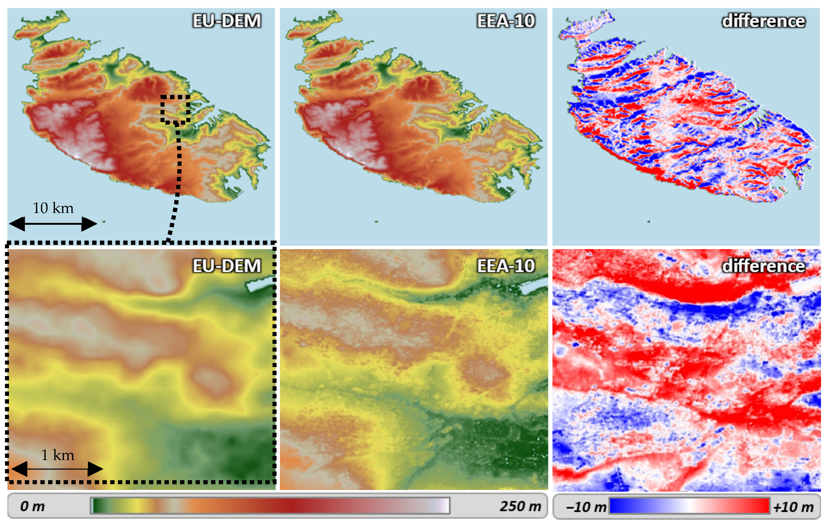
Abstract
:1. Introduction
1.1. Context
1.2. Effect of Planimetric Misregistration
1.3. Disparity Analysis
2. Methods
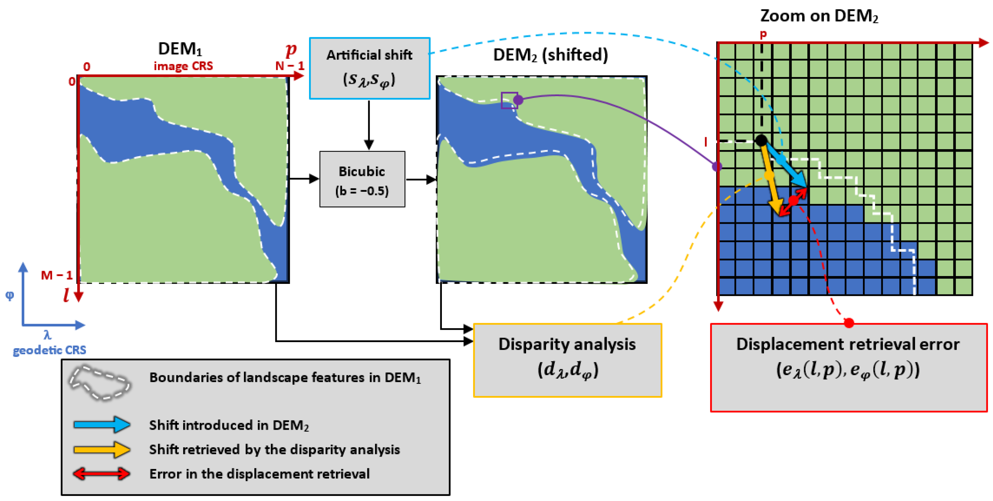
2.1. Principles
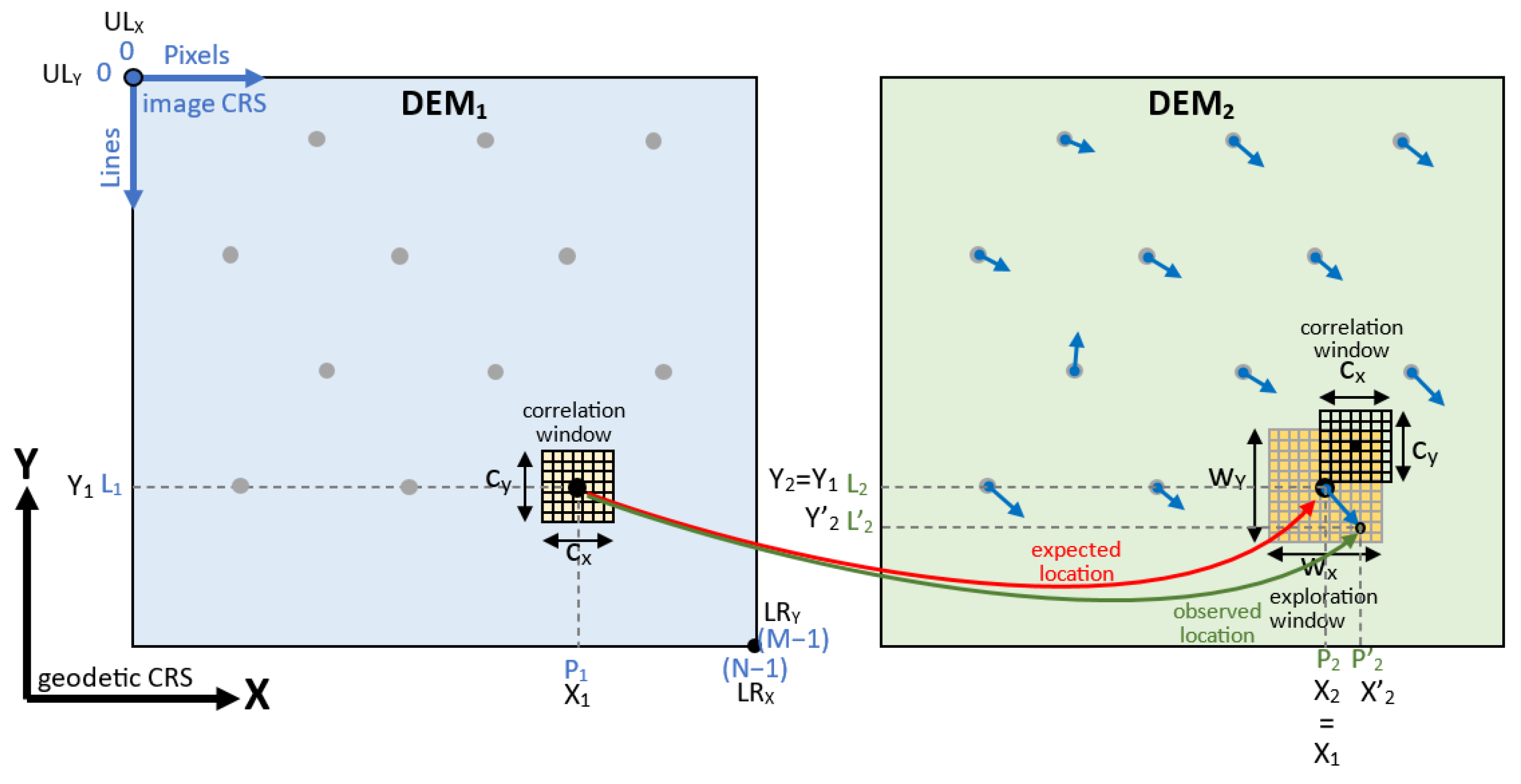
2.2. Pixel Matching
- r(dL,dP) is the linear regression coefficient computed at position (dL,dP) in the exploration window, i.e., between the correlation window around (L1,P1) of DEM1 and the correlation window around (L2 + dL,P2 + dP) of DEM2.
- Cov(DEM1(L1,P1),DEM2(L2 + dL,P2 + dP)) is the covariance computed between (L1,P1) of DEM1 and (L2 + dL,P2 + dP) of DEM2.
- σ1(L1,P1) is the standard deviation computed within a correlation window (cX × cY) centred on (L1,P1) in DEM1.
- σ2(L2 + dL,P2 + dP) is the standard deviation computed within a correlation window (cX × cY) centred on (L2 + dL,P2 + dP) in DEM2.

2.3. Sub-Pixel Matching
- x is the horizontal coordinate (longitude or easting) in the geodetic coordinates reference system. For geocoded images, this coordinate is given by x = ULX + PxGSDw (pixel width).
- y is the vertical coordinate (latitude or northing) in the geodetic coordinates reference system. For geocoded images, this coordinate is given by y = ULY − LxGSDh (pixel height).
- r(x,y) is the linear regression coefficient computed (for integer values as shown in previous section) or estimated using the paraboloidal interpolation (for sub-pixel floating values).
- R(X,Y) represents one of the 3 × 3 linear regression coefficients computed at pixel level, X = X0 − 1,X0,X0 + 1, Y = Y0 − 1,Y0,Y0 + 1.
- a,b,c,d,e,f are the 6 coefficients estimated from the 3 × 3 linear regression coefficients R(X,Y).
2.4. Choice of the Exploration and Correlation Window Sizes
3. Validation of the Sub-Pixel Displacement Retrieval
3.1. Principle
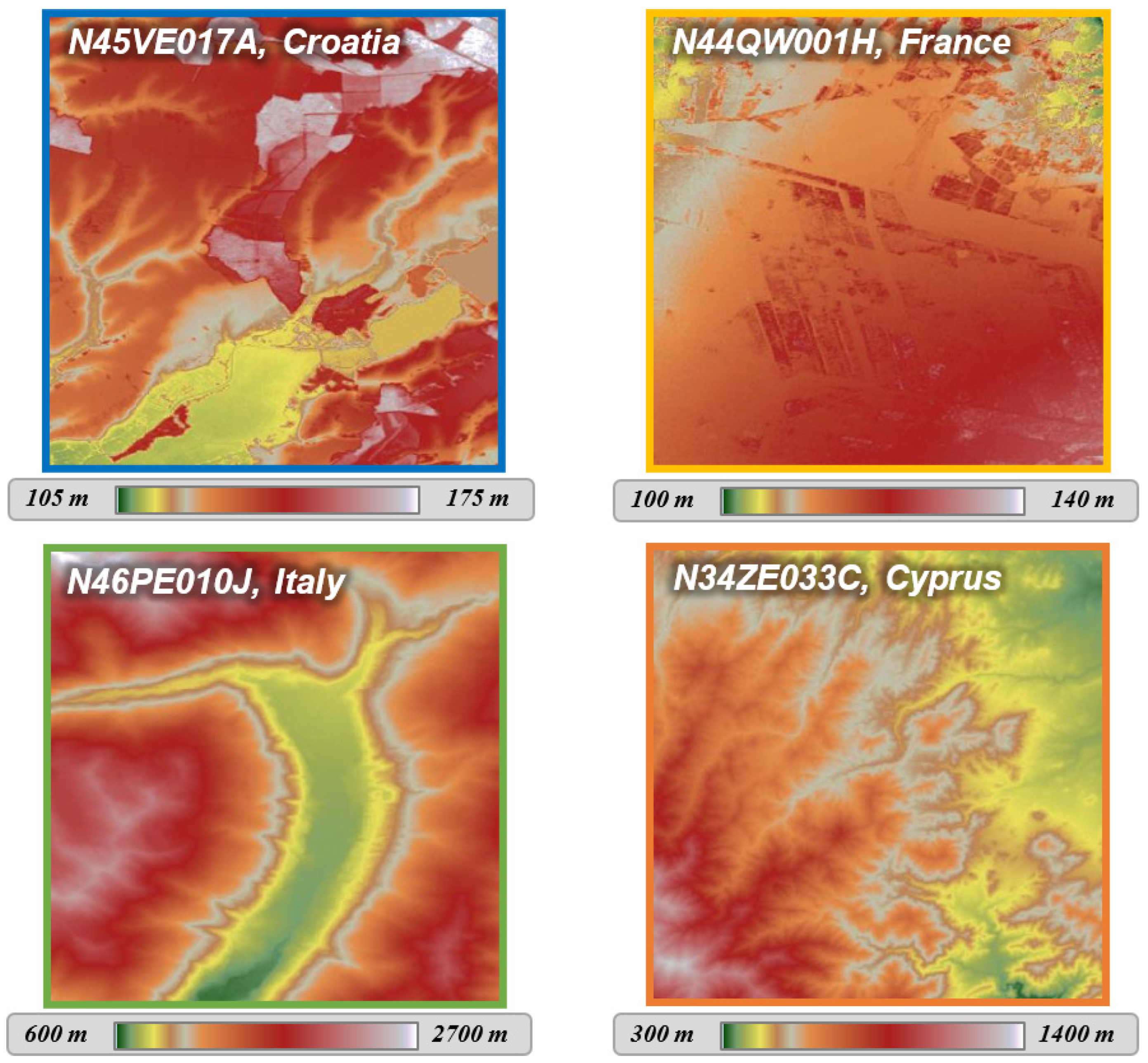
3.2. Study Areas
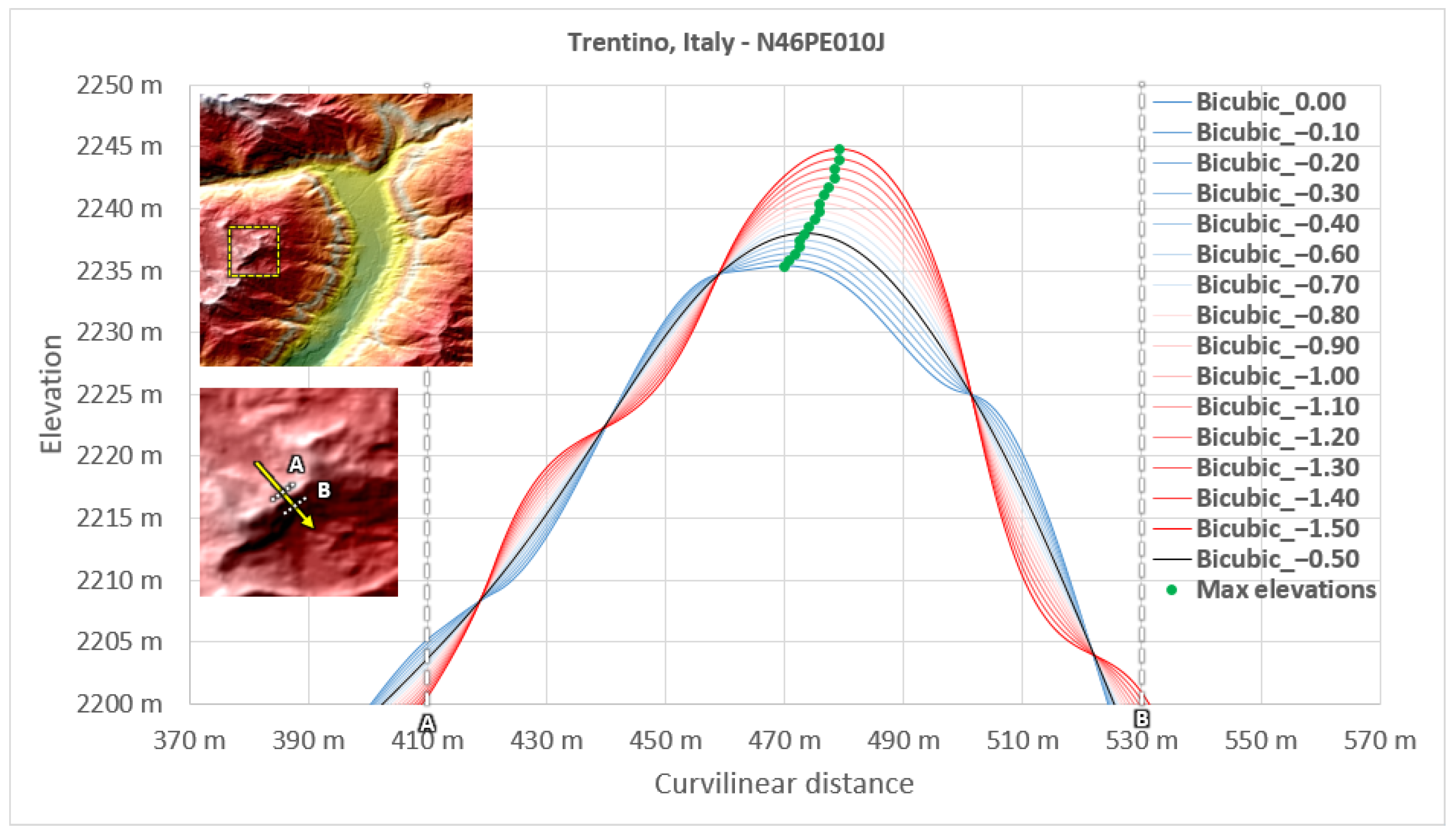
3.3. Bicubic Formula
3.4. Shift Validation
3.5. Error Matrices and Surfaces
3.6. Results
4. Finding the Best BiCubic (BBC) Parameter for Disparity Analysis
4.1. Principle
4.2. Displacement Error Graphs
4.3. Interpolation of the BBC
4.4. Results
5. Relation between BBC and DEM Slope Variations
5.1. Principle
5.2. Study Areas
5.3. Slopes Computation and Statistics
- DEM[l,p] is the elevation in the DEM in line l column p (in metres);
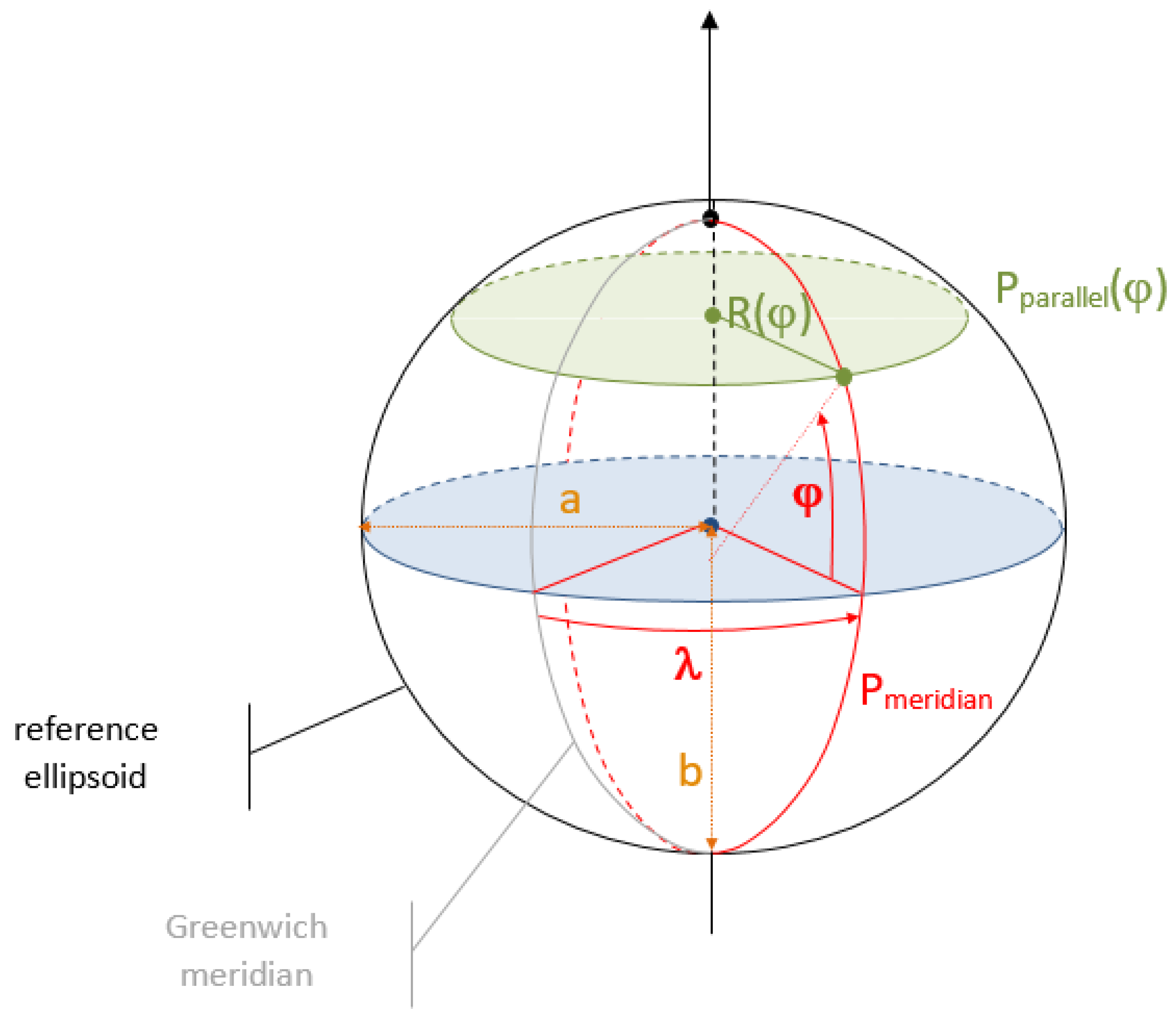
- Φ is the latitude;
- a is the semi-major axis of the ellipsoid;
- b is the semi-minor axis of the ellipsoid;
- GSDx is the horizontal ground sampling distance (in metres) (1);
- GSDy is the vertical ground sampling distance (in metres) (1);
- Δx is the horizontal angular resolution (in radians) (2);
- Δy is the vertical angular resolution (in radians) (2);
- Pparallel is the horizontal circumference of the ellipsoid at latitude φ;
- Pmeridian is the vertical circumference of the ellipsoid passing through the poles, approximately equal to 40,007.863 km for WGS84 ;
- e is the eccentricity of the ellipsoid.
- (1)
- Case of DEM expressed in a projected CRS, where x matches the Easting and y matches the Northing expressed in metres. In this case, Equations (24)–(28) are not needed.
- (2)
- Case of DEM expressed in the Geographic CRS (EPSG:4326), where x matches the longitude and y matches the latitude expressed in radians.

5.4. Logarithmic Correlation
- is the function predicting the best bicubic parameter.
- is the standard deviation of slope norm computed within the DEMIX tile.
5.5. Results
6. Discussion
7. Conclusions
Author Contributions
Funding
Data Availability Statement
Acknowledgments
Conflicts of Interest
Appendix A. Matrices and Surfaces of the Displacement Retrieval Errors


References
- Guth, P.; Van Niekerk, A.; Grohmann, C.; Muller, J.-P.; Hawker, L.; Florinsky, I.; Gesch, D.; Reuter, H.; Herrera, V.; Riazanoff, S.; et al. Digital Elevation Models: Terminology and Definitions. Remote Sens. 2021, 13, 3581. [Google Scholar] [CrossRef]
- Strobl, P.A.; Bielski, C.; Guth, P.L.; Grohmann, C.H.; Muller, J.-P.; López-Vázquez, C.; Gesch, D.B.; Amatulli, G.; Riazanoff, S.; Carabajal, C. The Digital Elevation Model Intercomparison Experiment Demix, A Community-Based Approach at Global Dem Benchmarking. Int. Arch. Photogramm. Remote Sens. Spat. Inf. Sci. 2021, XLIII-B4-2021, 395–400. [Google Scholar] [CrossRef]
- Guth, P.L.; Strobl, P.; Gross, K.; Riazanoff, S. DEMIX 10k Tile Data Set; Zenodo: Geneve, Switzerland, 2023. [Google Scholar] [CrossRef]
- Van Niel, T.; McVicar, T.; Li, L.; Gallant, J.; Yang, Q. The impact of misregistration on SRTM and DEM image differences. Remote Sens. Environ. 2008, 112, 2430–2442. [Google Scholar] [CrossRef]
- Hawwa, M.; Knudsen, T.; Kokkendorff, S.; Olsen, B.; Rosenkranz, B. Horizontal Accuracy of Digital Elevation Models; National Survey and Cadastre: Copenhagen, Denmark, 2011. [Google Scholar] [CrossRef]
- Mozas-Calvache, A.T. Positional Accuracy Assessment of Digital Elevation Models and 3D Vector Datasets Using Check-Surfaces. ISPRS Int. J. Geo-Inf. 2023, 12, 348. [Google Scholar] [CrossRef]
- Sutton, M.A.; Wolters, W.J.; Peters, W.H.; Ranson, W.F.; McNeill, S.R. Determination of displacements using an improved digital correlation method. Image Vis. Comput. 1983, 1, 133–139. [Google Scholar] [CrossRef]
- Barnard, S.; Thompson, W. Disparity Analysis of Images. Pattern Anal. Mach. Intell. IEEE Trans. 1980, PAMI-2, 333–340. [Google Scholar] [CrossRef] [PubMed]
- Guan, L.; Pan, H.; Zou, S.; Hu, J.; Zhu, X.; Zhou, P. The impact of horizontal errors on the accuracy of freely available Digital Elevation Models (DEMs). Int. J. Remote Sens. 2020, 41, 7383–7399. [Google Scholar] [CrossRef]
- Ghandehari, M.; Buttenfield, B.; Farmer, C. Comparing the accuracy of estimated terrain elevations across spatial resolution. Int. J. Remote Sens. 2019, 40, 5025–5049. [Google Scholar] [CrossRef]
- Keys, R. Cubic convolution interpolation for digital image processing. IEEE Trans Acoust Speech Signal Process. Acoust. Speech Signal Process. IEEE Trans. 1982, 29, 1153–1160. [Google Scholar] [CrossRef]
- Thevenaz, P.; Blu, T.; Unser, M. Interpolation revisited [medical images application]. IEEE Trans. Med. Imaging 2000, 19, 739–758. [Google Scholar] [CrossRef]
- Aganj, I.; Yeo, B.; Sabuncu, M.; Fischl, B. On Removing Interpolation and Resampling Artifacts in Rigid Image Registration. IEEE Trans. Image Process. 2013, 22, 816–827. [Google Scholar] [CrossRef] [PubMed]
- Lv, H.; Liu, Z.; Xu, B.; Cheng, B.; Hu, X. Interpolation Parameters in Inverse Distance-Weighted Interpolation Algorithm on DEM Interpolation Error. J. Sens. 2021, 2021, 3535195. [Google Scholar] [CrossRef]
- Shi, W.; Wang, B.; Tian, Y. Accuracy Analysis of Digital Elevation Model Relating to Spatial Resolution and Terrain Slope by Bilinear Interpolation. Math. Geosci. 2014, 46, 445–481. [Google Scholar] [CrossRef]
- Amante, C. Accuracy of Interpolated Bathymetric Digital Elevation Models; University of Colorado Boulder: Boulder, CO, USA, 2012. [Google Scholar]
- Zevenbergen, L.W.; Thorne, C.R. Quantitative analysis of land surface topography. Earth Surf. Process. Landf. 1987, 12, 47–56. [Google Scholar] [CrossRef]
- Ousguine, S.; Essannouni, F.; Essannouni, L.; Abbad, M.; Aboutajdine, D. A New Image Interpolation Using Laplacian Operator. In Advances in Ubiquitous Networking; Springer: Singapore, 2016; Volume 366, pp. 403–413. [Google Scholar] [CrossRef]
- Li, X.; Jiapei, H.; Liu, X.; Yu, J.; Feng, C. Adaptive digital elevation models construction method based on nonparametric regression. Trans. GIS 2022, 26, 2263–2282. [Google Scholar] [CrossRef]


Disclaimer/Publisher’s Note: The statements, opinions and data contained in all publications are solely those of the individual author(s) and contributor(s) and not of MDPI and/or the editor(s). MDPI and/or the editor(s) disclaim responsibility for any injury to people or property resulting from any ideas, methods, instructions or products referred to in the content. |
© 2024 by the authors. Licensee MDPI, Basel, Switzerland. This article is an open access article distributed under the terms and conditions of the Creative Commons Attribution (CC BY) license (https://creativecommons.org/licenses/by/4.0/).
Share and Cite
Riazanoff, S.; Corseaux, A.; Albinet, C.; Strobl, P.A.; López-Vázquez, C.; Guth, P.L.; Tadono, T. Best BiCubic Method to Compute the Planimetric Misregistration between Images with Sub-Pixel Accuracy: Application to Digital Elevation Models. ISPRS Int. J. Geo-Inf. 2024, 13, 96. https://doi.org/10.3390/ijgi13030096
Riazanoff S, Corseaux A, Albinet C, Strobl PA, López-Vázquez C, Guth PL, Tadono T. Best BiCubic Method to Compute the Planimetric Misregistration between Images with Sub-Pixel Accuracy: Application to Digital Elevation Models. ISPRS International Journal of Geo-Information. 2024; 13(3):96. https://doi.org/10.3390/ijgi13030096
Chicago/Turabian StyleRiazanoff, Serge, Axel Corseaux, Clément Albinet, Peter A. Strobl, Carlos López-Vázquez, Peter L. Guth, and Takeo Tadono. 2024. "Best BiCubic Method to Compute the Planimetric Misregistration between Images with Sub-Pixel Accuracy: Application to Digital Elevation Models" ISPRS International Journal of Geo-Information 13, no. 3: 96. https://doi.org/10.3390/ijgi13030096