Distinguishing the Intervalley Plain from the Intermountain Flat for Landform Mapping Using the Sightline Algorithm

Abstract

The intervalley plain is an important type of landform for mapping, and it has good connectivity for urban construction and development on the Loess Plateau. During the global landform mapping of the Deep-time Digital Earth (DDE) Big Science Program, it was found that slope and relief amplitude hardly distinguished intervalley plains from intermountain flats. This study established a novel descriptive method based on a digital elevation model to describe the difference between intervalley plains and intermountain flats. With the proposed method, first the pattern of variation in the elevation angle is described using a sight line on the terrain profile, and the lowest elevation angle (LEA) is extracted. The maximum value of the LEA is subsequently used among multiple terrain profiles to represent the maximum velocity of the elevation decrease, that is, the three-dimensional lowest elevation angle (3D LEA), to represent the intervalley plains with lower 3D LEA values. The sight parameters of the 3D LEA are evaluated to optimize the intervalley plain mapping. The functional mechanism of the sight parameters is presented from a mathematical perspective and a comparative analysis of the 3D LEA is performed for the relief amplitude and slope angle at multiple scales. This study explores sight-line analysis in a novel way, providing a new terrain factor for landform mapping involving intervalley plains.

1. Introduction

An intervalley plain is a basic element of landform mapping and an important land resource for urban development. Any landform has a certain form that reflects the characteristics of the development and evolution of the landform at a certain moment, and the morphology can be characterized by a digital elevation model (DEM) [1]. In previous studies, plains were often judged by the slope and relief amplitude of the terrain. The Committee on Geomorphic Survey and Mapping (CGSM) specifies plains (0–0.5°), slight slopes (0.5–2°), gentle slopes (2–5°), slopes (5–15°), steep slopes (15–35°), scarps (35–55°), and vertical walls (55–90°) [2]. Chen and Han applied a relief amplitude of less than 30 m to determine the range of a plain [3,4]. Hu and Nie defined a plain as having a relief amplitude of no more than 30 m [5]. Sun classified relief amplitudes as plains if they were less than 20 m [6]. Zeng classified plains based on both slope and relief amplitude, with a slope of 2° and an undulation of 20 m [7].

In the past two years, Nanjing Normal University has conducted global landform mapping research under the framework of the Deep-time Digital Earth (DDE) Big Science Program. However, significant problems were encountered when extracting plains based on slope and relief amplitude. At the regional scale, the Earth’s surface has relatively flat components within mountains, resulting in the presence of low-value zones of slope and relief amplitude. Plains extracted by slope and relief amplitude not only contain intervalley plains but also many pseudoplains caused by intermountain flats, which necessitates a significant amount of removal work. Therefore, constructing new terrain factors to replace or supplement slope and relief amplitudes is highly important for regional landform mapping.

Previous researchers have conducted extensive research on the automatic classification of landforms based on terrain factors. Wood established standards based on four morphological parameters (slope, cross-sectional curvature, maximum curvature, and minimum curvature), dividing the land surface into six elements: channels, ridges, planes, peaks, pits, and saddles [8]. Ehsani and Quiel combined the four morphological parameters mentioned above into a 4-dimensional vector as the input vector for self-organizing mapping (SOM) and trained SOM to classify landform elements on the surface [9]. Yan applied the SOM method to loess-landform mapping and found that eight elements are suitable for loess areas [10]. Unlike previous methods, Jasiewicz and Stepinski abandoned slopes and proposed a geomorphon method based on line-of-sight analysis [11]. This method evaluates the changes in elevation in eight directions, namely north, northeast, east, southeast, south, southwest, west, and northwest, and it identifies ten basic elements: slope, ridge, valley, flat, spur, hollow, shoulder, footslope, peak, and pit. The geomorphon method has been widely applied in the study of various landforms such as glacial landforms, submarine landforms, and loess landforms [12,13,14,15,16,17,18,19,20]. However, it is unclear whether the line of sight can replace the slope and relief amplitude for identifying intervalley plains.

The aim of this study was to develop sight-line algorithms to distinguish intervalley plains from intermountain flats. A quantitative indicator, 3D LEA, is generated by the sight-line algorithm and optimized by analyzing the impact of sight parameters such as the sight direction, distance, and skip radius for intervalley plain identification.

2. Study Area and Data

The Loess Plateau is widely developed with loess ridges, dense gullies, and relatively scarce flat terrain suitable for construction. The intervalley plain in the Loess Plateau region is low and flat, adjacent to the Yellow River system, and has good connectivity for urban construction and development in the loess ridge and hill region. The distribution of intervalley plains is highly important for estimating land resources for urban development on the Loess Plateau. The intervalley plain is close to water sources, and many important towns on the Loess Plateau have to develop along the intervalley plain. It is important to explore the spatial distribution of intervalley plains on the Loess Plateau and promote urban development along the valley. Previous studies have focused more on extracting gully shoulder lines, which indicate the boundaries of soil erosion on the Loess Plateau. The literature has divided loess gullies into positive and negative terrains. The gully shoulder line is the middle boundary between the negative and positive terrains. Many extraction methods proposed by previous researchers [21,22,23] have been developed for high-resolution DEMs to improve the extraction accuracy for gully shoulder lines. Several scholars have focused on the extraction of tablelands or highlands [24,25]. Unlike previous studies, this study focused on the extraction of Loess Intervalley Plain data.

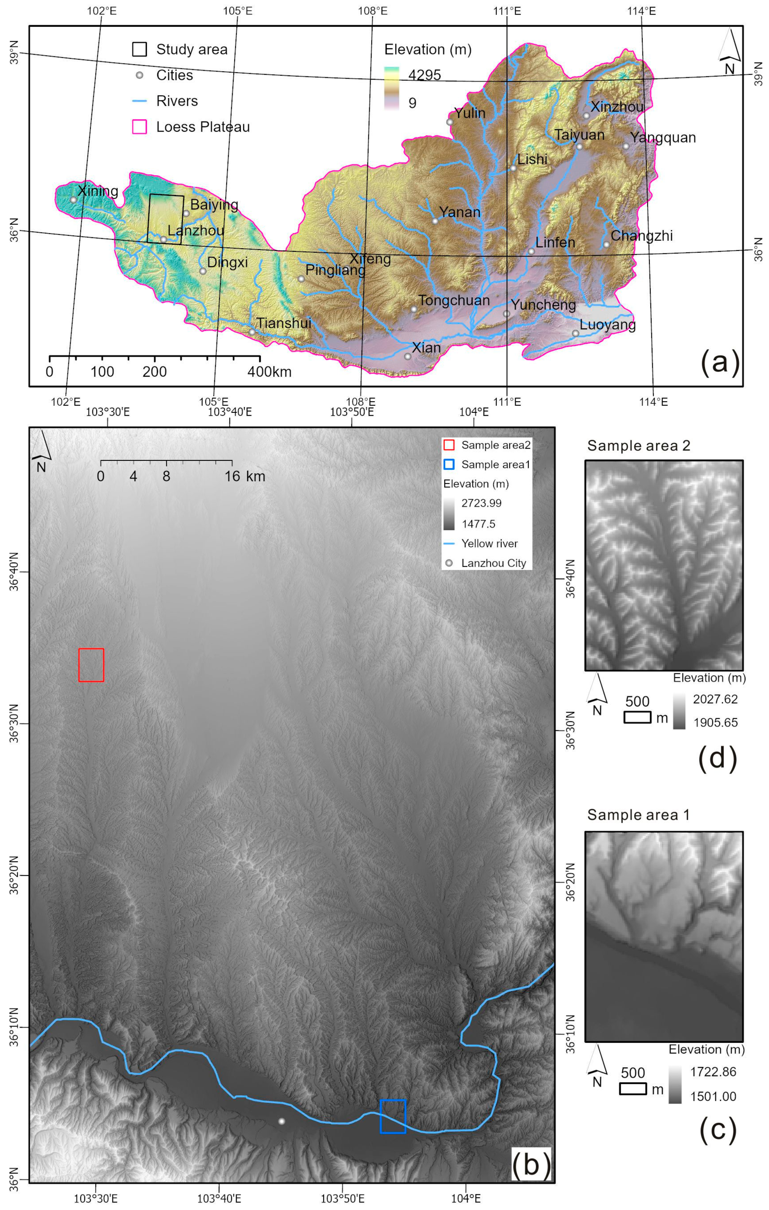
Lanzhou city is located in the geometric center of Northwest China and mainland China. The terrain is high in the west and south and low in the northeast. Lanzhou has benefited from the Silk Road and has become an important transportation hub and commercial port. It was identified as one of the key industrial bases for construction, becoming an important national base for petrochemical, biopharmaceutical, and equipment manufacturing. In 2012, the State Council approved the construction of the Lanzhou New Area, the first national-level new area in the northwestern region, as an important measure for deepening the implementation of the Western Development Strategy.

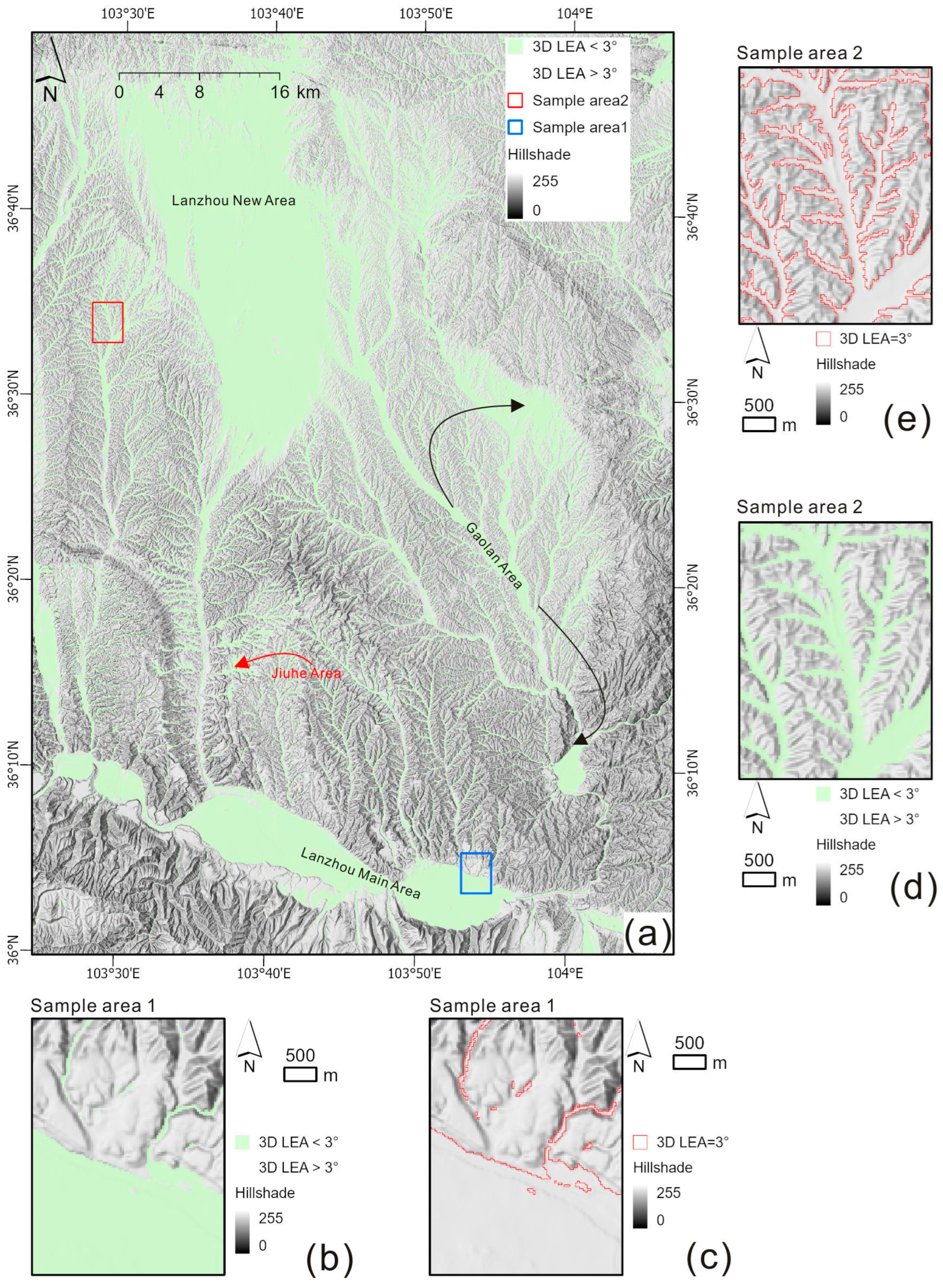
Lanzhou and surrounding areas were selected as examples for conducting research on the extraction of intervalley plains. The case area is located at 103°24′–104°6′ E, 36°00′–36°50′ N (Figure 1). The southern part includes two intervalley basins containing the urban area of Lanzhou, through which the Yellow River flows. The northwest region is the location of the Lanzhou New Area. The Lanzhou New Area has a total area of 1744 square kilometers, and as of the end of 2021, the permanent population of the Lanzhou New Area was 300,000. Two sample areas were selected for the presentation of extraction details. Sample area 1 is located at the northern boundary of the intervalley basin in the main urban area of Lanzhou. Sample area 2 is located in the valley, which is near the new Lanzhou area. The DEM data were obtained from FABDEM [26], which was used as the data source for DDE’s global landform mapping and was provided by the University of Bristol in 2021 and downloaded from the website https://data.bris.ac.uk/data/dataset (accessed on 1 May 2022). The precision is approximately 3–14 m with a resolution of 1″ and two significant decimal places. The data are projected onto a WGS1984 48 N grid with a size of 30 m. Figure 1c,d shows the locally amplified FABDEM for the sample areas. The Yellow River in sample area 1 cuts the intervalley plain near the northern foothills, whereas the valley bottom is basically flat for sample area 2.

3. Methodology

3.1. Problems Faced with Slope and Relief Amplitude

For the DEMs, the early built-in slope tool in ArcGIS was the linear regression-plane method at the 3 × 3 window scale. Subsequently, GRASS GIS has integrated Wood’s unweighted quadratic surface, providing the slope calculation tool “r.param.scale” for different window sizes from 3 × 3 to 499 × 499. The latest ArcGISpro provides a surface parameter tool that can calculate slopes for different window sizes of 3 × 3–15 × 15, with the aim of smoothing laser point-cloud data noise. The slope tool approximates the slope by fitting a plane to nine nearby cells [27] and it may not accurately represent the landscape, as it can potentially obscure or amplify important natural variations. The GRASS GIS and ArcGIS Surface Parameters tools fit a surface to the surrounding cells, resulting in smooth terrain. The relief amplitude also displays significant scale dependence and is commonly used for landform classification [28,29]. Therefore, slope and relief amplitude issues at multiple scales are also the focus of this study.

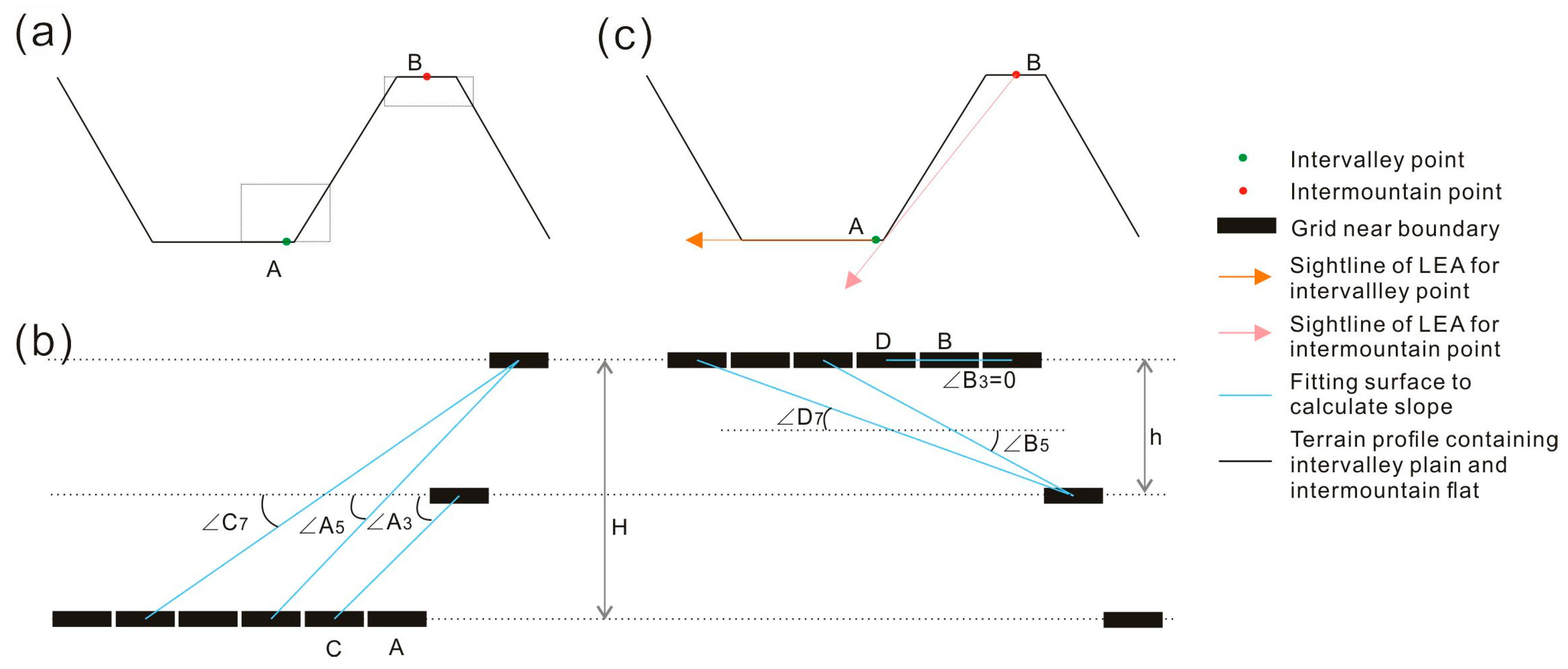
Figure 2 illustrates the problem of extracting pseudo plains within mountains via slope and relief-amplitude data. Point A is the point on the intervalley plain, and point B is the point on the intermountain flat. The values of relief amplitude and slope depend on the distance from the hillslope. In Figure 2a, point A is closer to the hillslope than point B is, so larger values of slope tends to be obtained. In Figure 2b, the grids are used to represent the local terrain profile in detail. When the window size is 3 × 3, the slope of A “∠A₃” is greater than the slope of B “∠B₃”. For dividing a plain with a critical slope value, if point A is to be classified as a plain, then this critical value must be greater than “∠A₃” and also greater than “∠B₃”. When the window size is 5 × 5, “∠A₅” is also greater than “∠B₅”, and point B is also classified as a plain. If the size is chosen to be 7 × 7, then similar situations occur at points C and D. If C is to be classified as a plain, then D is also classified as a plain, because “∠C₇” is greater than “∠D₇”.

For relief amplitude, point B is more easily divided into plains than point A. When the window is 3 × 3, the fluctuation in point A is equal to H-h, while the fluctuation in point B is 0. When the window size is 5 × 5, the fluctuation in point A is H, while the fluctuation in point B is h and lower than H. When the window size is 7 × 7, the fluctuation in C is H, while the fluctuation in D is h. C is more difficult to divide into plains than is D. Similarly, the change in window size cannot solve the problem that the boundary of intervalley plains is more difficult to classify as plains than is the center of flat components within mountains.

3.2. Positioning an Intervalley Plane Using LEA in a 2D Profile

The sight line seems to avoid this problem, as indicated in Figure 2c. The sight line defines the lowest (minimum) elevation angle (LEA) and maximum elevation angle (MEA) [30]. Figure 2c introduces sight lines to present the distribution of the lowest elevation angle (LEA) along the 2D profile. Due to the elevation difference of hillslopes, the LEA of point B is much larger than that of point A. Therefore, when setting a critical LEA to attribute A to the plain, this critical value can be smaller than B’s LEA, avoiding attributing B to the plain.

Figure 3 compares LEA and MEA within a profile from the upper hill to the lower valley. The top part, AB, is a hillslope with large undulations and steep slopes, and the bottom part, CD, is an intervalley plain that is nearly horizontal. Because the slope of the terrain profile decreases from top to bottom, the LEA values in sections AB, BC, and CD are different. As shown in Figure 3, the LEA of point H is greater than that of point F even though they are near point B. The LEA of point F is greater than that of point P even though they are near point C. Therefore, the LEA can reflect the slope changes near the footslope BC. At the hill peak, even if it is relatively flat, there is still a relatively large LEA. In contrast to that of the LEA, the maximum elevation angle (MEA) of the footslope was not able to change with slope because the MEA at point H was similar to that at F when the two points were near B, and the MEA at point F was similar to that at P when they were near C (Figure 3).

3.3. Calculation of 2D LEAs

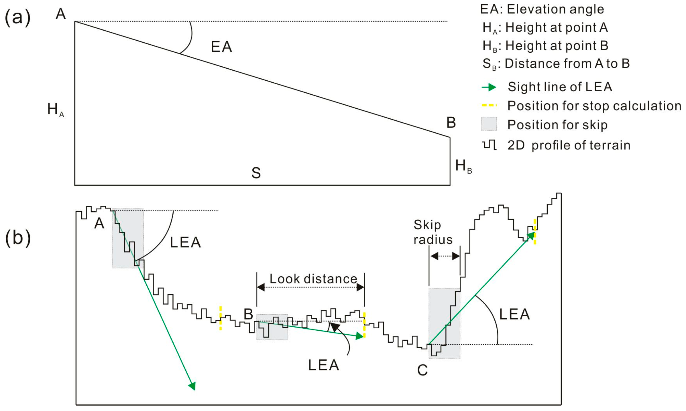
The calculation of the elevation angle (EA) between the traversal grid and the central grid is shown in Figure 4a. The calculation formula for the elevation angle of neighborhood unit B to A is

$$\mathrm{E}\mathrm{A}=\mathrm{a}\mathrm{r}\mathrm{c}\mathrm{t}\mathrm{a}\mathrm{n} \left(\frac{{\mathrm{H}}_{\mathrm{B}}-{\mathrm{H}}_{\mathrm{A}}}{\mathrm{S}}\right)\ast 57.29578$$

(1)

where EA is the elevation angle in degrees; ${\mathrm{H}}_{\mathrm{B}}$ and ${\mathrm{H}}_{\mathrm{A}}$ are the elevations of the neighborhood unit (B) and the center unit (A), respectively; and S is the distance between point B and point A. The elevation of A is the original elevation that was not traversed. The elevation of B is obtained by traversing the 2D profile using the convolution approach. The range of elevation angle values is [−90, 90]. A negative value indicates that point B is at the oblique downward position of A.

To calculate the 2D LEA, it is necessary to further compare all elevation angles obtained by traversing the 2D profile (Figure 4b). Then, the opposite number of minimum values is used as the lowest elevation angle (LEA) in this direction. The value range of the LEA is also [−90, 90]. A positive value indicates that the sight line of LEA is downward, while a negative value indicates that the sight line is upward. A value of 0 indicates that a line of view is basically horizontal. The formula for calculating the LEA in each direction is given as follows:

$${\mathrm{L}\mathrm{E}\mathrm{A}}_{\mathrm{i}}=-\mathrm{m}\mathrm{i}\mathrm{n}({\mathrm{E}\mathrm{A}}_{\mathrm{i}}^1,{\mathrm{E}\mathrm{A}}_{\mathrm{i}}^2,{\mathrm{E}\mathrm{A}}_{\mathrm{i}}^{\mathrm{j}},\dots ,{\mathrm{E}\mathrm{A}}_{\mathrm{i}}^{\mathrm{m}})$$

(2)

where ${\mathrm{L}\mathrm{E}\mathrm{A}}_{\mathrm{i}}$ represents the lowest elevation angle to be solved in the ith direction. ${\mathrm{E}\mathrm{A}}_{\mathrm{i}}^{\mathrm{j}}$ represents the elevation angle calculated for the jth grid in the ith direction. m is the maximum number of grids, depending on the size of the analysis scale. Therefore, LEA can consider the slope of a surface at a relatively global scale rather than at a local analysis window.

3.4. Three-Dimensional LEA Calculation

Figure 4 shows a 2D profile of the terrain, whereas the actual terrain exists in 3D space. The direction of the profile usually needs to be along the inclination to ensure that the LEA is the largest in 3D space. Therefore, it is necessary to test different directions to determine the three-dimensional lowest elevation angle, abbreviated as 3D LEA.

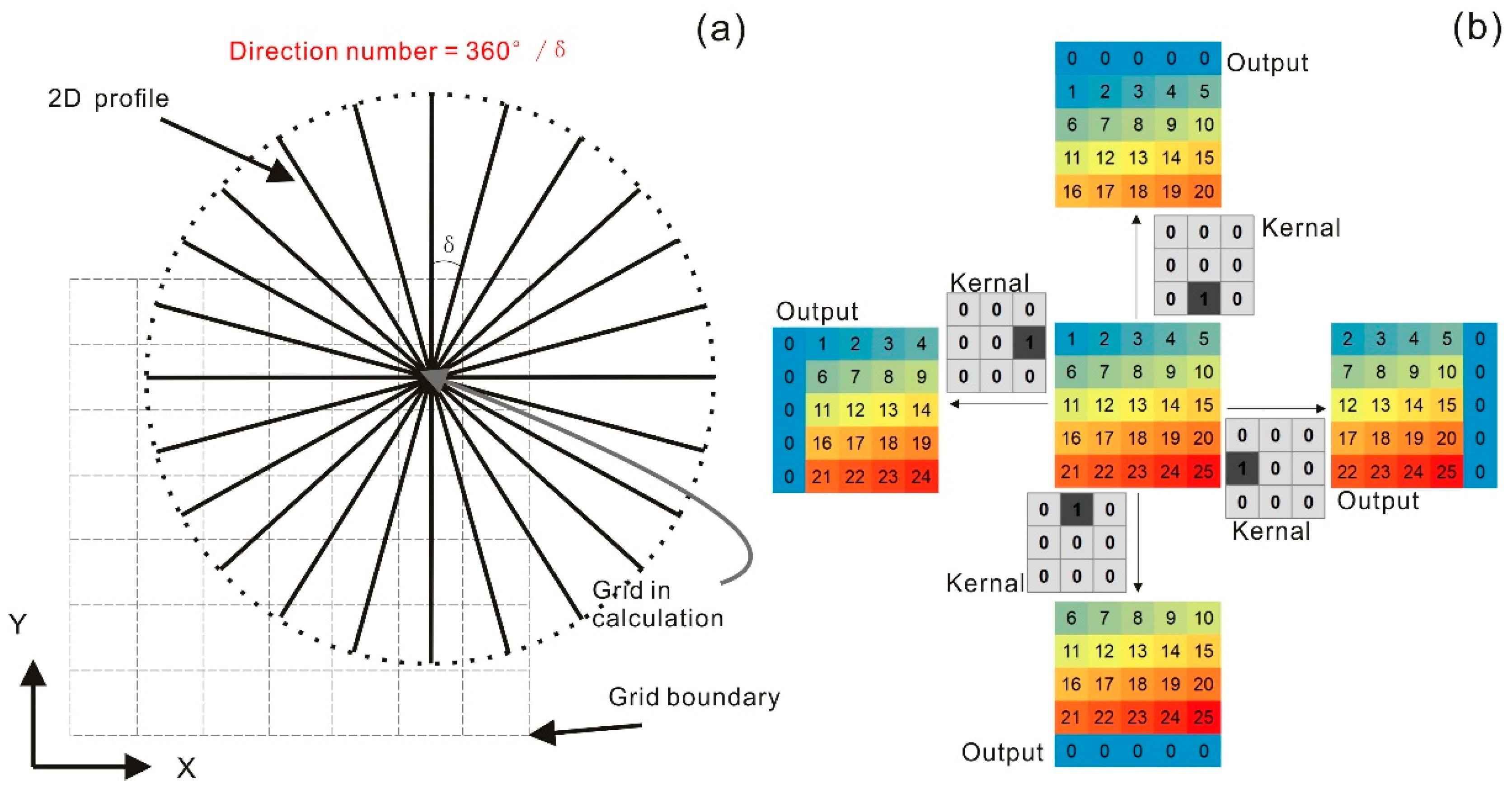
Figure 5a shows a schematic diagram of multidirectional traversal. The azimuth of 0–360° is first divided into a certain number of directions at a specific interval. By setting a sufficiently small interval, the 3D LEA is obtained by calculating the elevation changes in as many directions as possible. The maximum value of LEAs in multiple directions is taken as the 3D LEA, and the calculation formula is given as follows:

$$3\mathrm{D}\mathrm{L}\mathrm{E}\mathrm{A}=\mathrm{m}\mathrm{a}\mathrm{x}({\mathrm{L}\mathrm{E}\mathrm{A}}_1,{\mathrm{L}\mathrm{E}\mathrm{A}}_2,{\mathrm{L}\mathrm{E}\mathrm{A}}_{\mathrm{i}},\dots ,{\mathrm{L}\mathrm{E}\mathrm{A}}_{\mathrm{n}})$$

(3)

where n is the number of directions. The numerical range of the 3D LEA is [−90, 90]. A positive value indicates that at least one neighborhood grid is lower than the central grid. A negative value indicates that all neighborhood grids are higher than the central grid.

The traversing of the DEM matrix can be implemented by convolution operations in all four compass directions: north, east, west, and south. Figure 5b shows a schematic diagram of the convolution movement principle for the four main compass directions. Notably, there are no data outside the DEM range, and the value changes to 0 after the grid at the boundary is moved. Therefore, the loaded DEM data must be larger than the target area; this effect is considered the “edge effect” during computational experiments on digital elevation models.

When the interval is 45°, the DEM is traversed in eight compass directions. Additional directions, including the northeast, northwest, southeast, and southwest, can be combined with the four main compass directions. For example, the northeast direction can be combined with the east and north directions once each. When the interval is less than 45°, traversing in any direction requires the combination of multiple convolution kernels. The 3D LEA-calculation script was written in MATLAB 2020. Due to the independent nature of multidirectional computations, the computation time depends on the time required for traversing in one direction when the number of CPU cores and the amount of memory are large enough.

3.5. Sight Parameters Affecting 3D LEA

Three parameters affect the 3D LEA: direction number (Figure 5a), look distance, and skip radius (Figure 4b).

The first parameter is the number of directions that need to be considered when using the multidirectional traversal mode. The greater the number of directions is, the closer the result calculated by the multidirectional traversal mode is to the ideal 3D LEA.

The second parameter is the look distance, which determines the allowable length of the terrain profile. Relatively large look distances can be used to calculate 3D LEAs at a relatively global scale; accordingly, the results are also on a relatively macro scale. However, the greater the look distance is, the greater the amount of computation required. For parallel computation of CPU i7 10700, it takes approximately 0.1 million grids per second when look distance is 3000 m.

The third parameter is the skip radius, which filters out terrain changes in areas very close to the central grid. Due to the inevitable inclusion of abnormal elevation information in DEM data, when this information is very close to the central grid, and because the distance S between the grids is very small, the impact of this abnormal information on the LEA calculation will increase.

3.6. Critical 3D LEA for the Intervalley Plain

After the 3D LEA was calculated, the critical value was determined for the 3D LEA through human interpretation to obtain the intervalley plain. Overall, the 3D LEA layer was overlaid on the hillshade, and the transparency was set to 30% in ArcGIS. The intervalley plain should contain a low value of 3D LEA, while the sloping land should host a relatively larger 3D LEA. Therefore, by setting a threshold value, the intervalley plain can be recognized.

However, in reality this process is very complex. As mentioned earlier, three sight parameters simultaneously affect the 3D LEA. The critical value that leads to the differentiation of intervalley plains may also be uncertain. For example, when we set different skip radii, the threshold values may be different. According to the literature [8] and our previous experience, slopes of 2–5° can be used as slope thresholds for dividing mountains and plains. This study divides 3D LEAs into eight segments at 1-degree intervals, namely, below 1°, 1–2°, 2–3°, 3–4°, 4–5°, 5–6°, 6–7°, and above 7°, which are expected to contain the threshold of the intervalley plain. By observing which segments are included in the intervalley plain, we can roughly determine the threshold and select the appropriate part as the intervalley plain. In addition, the influence of sight parameters on the threshold may also be considered.

4. Results

4.1. Influence of Direction on 3D LEAs

The terrain has anisotropic characteristics, and multiple directions must be used to resolve azimuth bias [31,32,33]. Yokoyama et al. (2002) calculated the elevation angles and nadir/zenith angles of eight compass directions to describe surface morphology [30]. Prima et al. (2006) classified volcano landform types from nadir and zenith angles in eight directions [34]. Jasiewicz and Stepinski [11] mapped ten landform elements based on the difference between the nadir and zenith angles from eight compass directions. Other studies have shown that the extraction of loess gully shoulder lines is relatively complete when 12 directions are used [22,23]. 3D LEA is used to integrate multiple directions of LEA to distinguish between sloping land and intervalley plains.

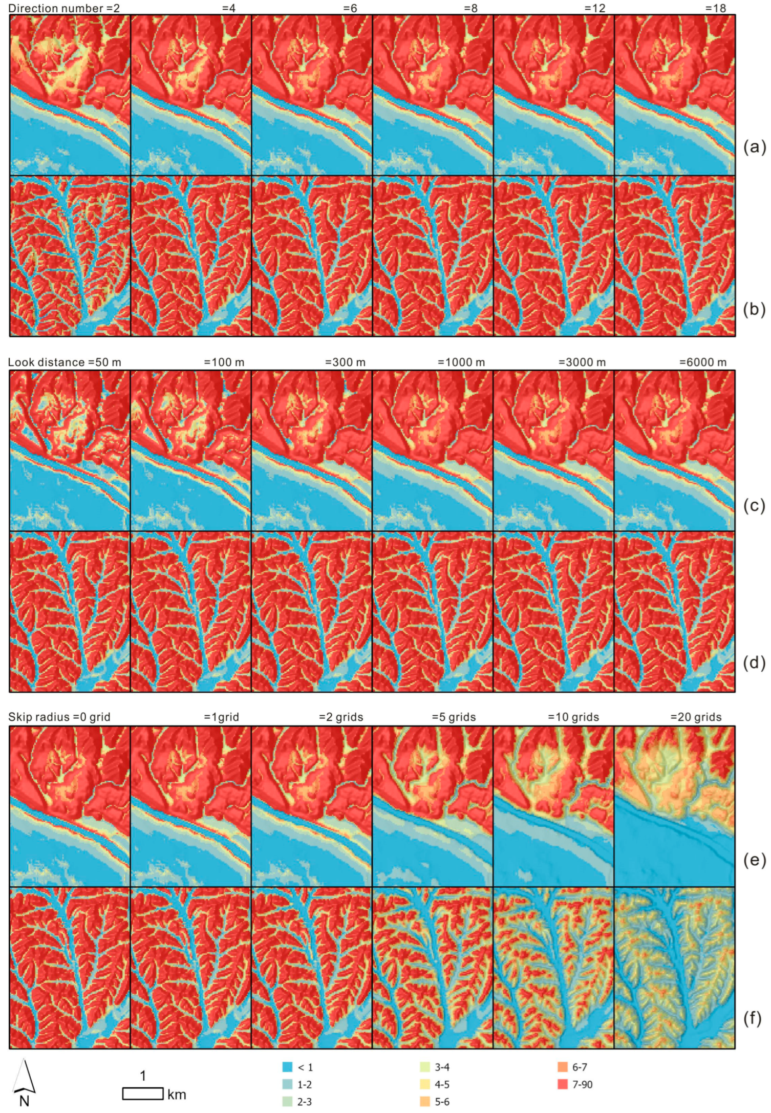
Figure 6 shows the change in the 3D LEA with the number of directions, with a fixed skip radius of 0 m and a look distance of 3000 m. When the number of directions increases from two to six, there is a significant change in the distribution of the 3D LEA. For sample area 1, the area of low 3D LEAs on the hillslope decreases significantly, and there is little change when the number of directions is greater than six. For sample area 2, there is a significant difference between the two directions and the four directions, and as the number of directions continues to increase, the small patches formed by low values of 3D LEA inside the hillslope gradually decrease.

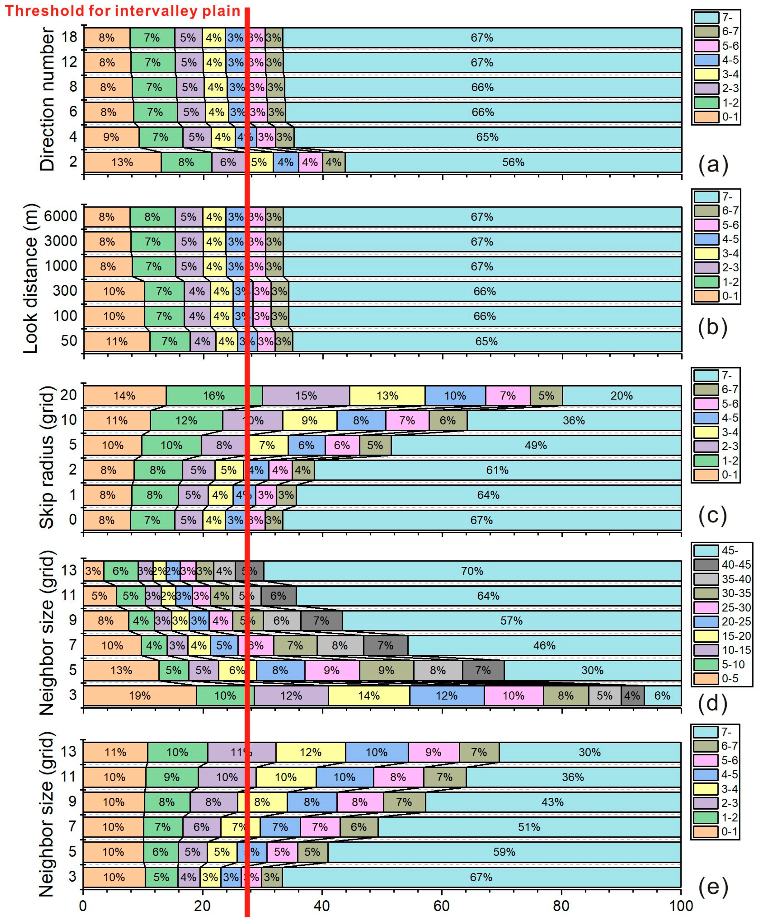
Figure 7 shows the statistical results for various 3D LEAs in the entire research area. As the number of directions increases, the area of 3D LEAs above 7° increases. Especially from two directions to six directions, changes are the most meditative. After reaching six directions, the changes in 3D LEAs are relatively small. According to previous research [11,22,23], 8 directions is considered the minimum number of directions, and 12 directions are recommended. The following analysis will uniformly set 12 directions.

4.2. Influence of Look Distance on 3D LEAs

The look distance controls the analysis scale of 3D LEAs. When the observation distance is 50 m, calculations are equivalent to calculations under the 3 × 3 window. The local undulation of terrain controls the value of 3D LEA, causing many low values to appear on gentle hillslopes. The pseudo plain within the mountain will also be extracted because it does not reach the scale of the pseudo plain within the mountain. For sample area 1, there are relatively large terraces on the hillside, with low 3D LEA values converging into large blocks (Figure 6c). For sample area 2, there are many small fragments on the hillside (Figure 6d). As the look distance increases, the low-value areas within the hillslope gradually shrink and disappear, causing the removal of pseudoplains. When the distance exceeds 1000 m, the change in the 3D LEA distribution is not significant, and the area of the pseudoplain does not decrease. It is believed that above 1000 m the content of pseudo plains within the mountain is greatly reduced. The statistical results indicate that the area of 3D LEAs above 7° in the entire study area increased from 65% for a look distance of 50 m to 67% for a look distance of 1000 m. After 1000 m, the overall change was relatively small (Figure 7b). In addition, as the look distance increases from 50 m to 1000 m, the 3D LEA gradually increases in the plains on both sides of the deep cutting channel.

There should be a minimum analysis window requirement for analyzing the surface morphology of the Loess Plateau. For the research area, the minimum look distance is 1000 m. This result is slightly lower than that of the study by Jasiewicz and Stepinski [11], who believe that a minimum look distance of 1500 m is necessary. This result also reflects the dense distribution of loess gullies and the small spacing between gullies due to cutting and fragmentation. In addition, the look distance required for identifying underwater geomorphic elements in the Yangtze River can reach 100 m [35]. Compared to that on the riverbed topography, the look distance on the Loess Plateau is much greater. Considering the small computational burden, we suggest setting a larger look distance that will be uniformly set to 3000 m for the following analysis.

4.3. Intervalley Plain Extraction

4.3.1. Influence of Skip Radius on 3D LEAs

The skip radius can smooth 3D LEAs and effectively filter out some small outliers. The local high values that appear within the intervalley plain of sample area 1 gradually decrease with increasing skip radius, especially for the banded 3D LEA with high values on both sides of the deep cutting channel. When the skip radius is 20 grids, the 3D LEA of the intervalley plain is less than 1°. The skip radius of 20 grids also has a significant impact on the boundary morphology of the 3D LEA classification, resulting in a significant deviation in the boundaries of the valley plain. Therefore, it is not suitable to use a particularly large skip radius. The increase in the skip radius also resulted in a decrease in the overall 3D LEA (Figure 6e). Similar phenomena also occur in sample area 2, where the overall 3D LEA decreases as the skip radius increases (Figure 6f). Therefore, an appropriate skip radius is necessary, and five grids are recommended because these artifacts are generally eliminated.

The statistical results also indicate that the impact of the skip radius on 3D LEAs is significant and persistent. A 3D LEA above 7° decreases from 67% at a skip radius of 0 to 20% at a skip radius of 20 grids. The decrease is approximately 2.3–2.4%/grid. When the skip radius is from 2 to 5, the decrease is the greatest, reaching 4%/grid. However, the 3D LEA at 0–5° increases from 27% to 68%, which is the most significant increase (Figure 7c). This indicates that as the skip radius increases the 3D LEA decreases to less than 5° for most areas.

4.3.2. The Threshold Value for the Intervalley Plain

Figure 8 shows the distribution of 3D LEAs below 3° when the skip radius is five grids. Overall, the low 3D LEA value is consistent with the spatial distribution characteristics of the intervalley plain in the study area, especially for the intervalley basins in the main urban area of Lanzhou and the plains in the new Lanzhou area. Moreover, the width of the intervalley plains varies for different developed gullies within the study area. The relatively wide intervalley plain in the east is the location of Gaolan County. For the mountain area on the southern edge, there is almost no intervalley plain, which limits the expansion of Lanzhou city. Therefore, when the skip radius is five grids, 3° can be considered the critical value for distinguishing between intervalley plains and mountains/hillslopes that may contain flat components.

As mentioned earlier, skipping the radius will change the distribution of 3D LEAs. Assuming that the area of the intervalley plain remains constant, the critical value should change with the change in the skip radius. Figure 7c depicts the reference threshold line. When the skip radius is 0, setting the critical value to 5° is more appropriate. When the skip radius is 10 grids, the critical value should not exceed 2.5°, while when the skip radius is 20 grids, the critical value should be smaller, that is, approximately 1.8°.

5. Discussion

5.1. Explanation of the Computer-Sight Parameters

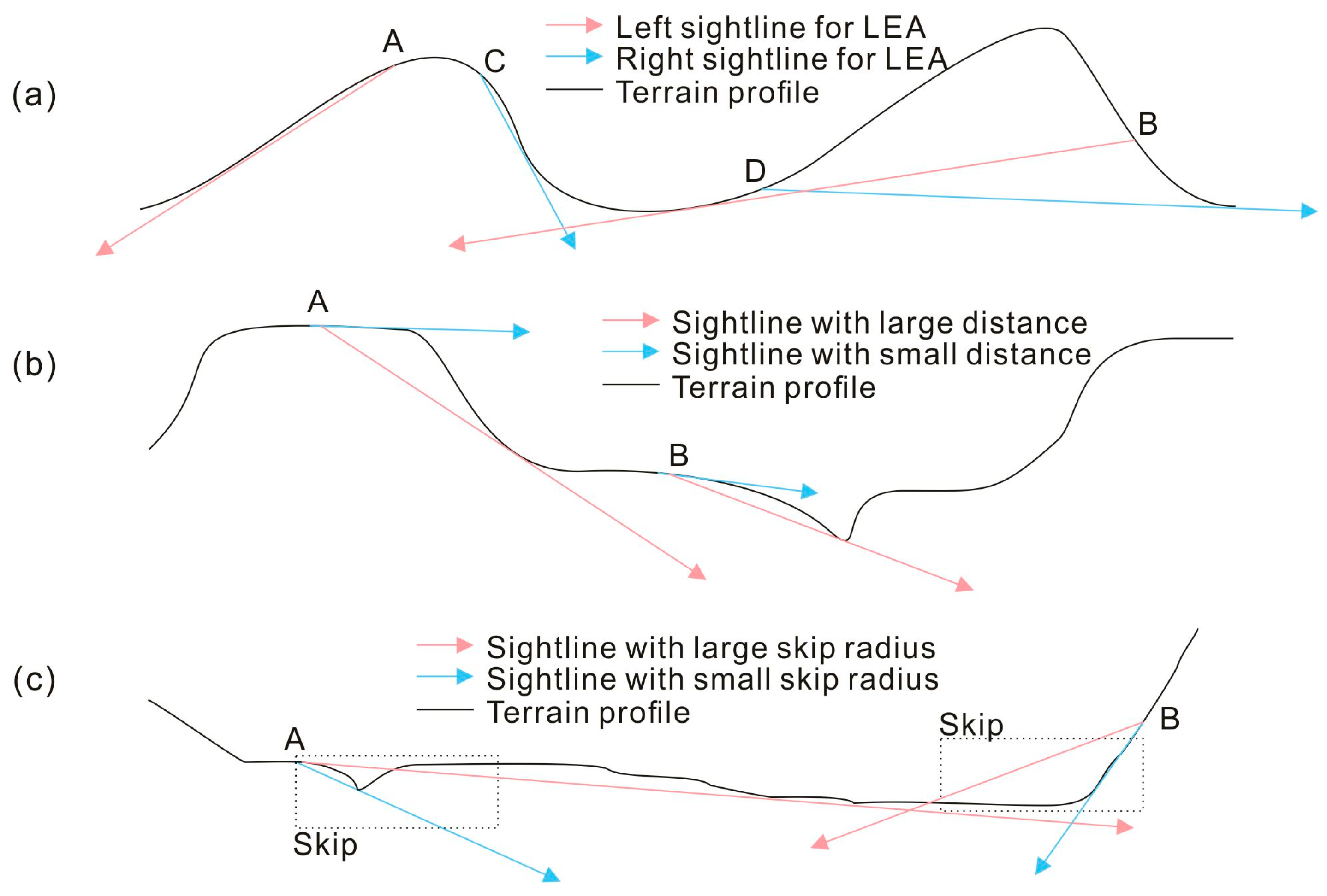
Below, the impact of the abovementioned sight parameters on the 3D LEA calculation is explained through a terrain profile (Figure 9). First, the sight direction affects the distribution of LEA, and only slopes that tend to have the same direction have a large LEA value. The central grid for the blue line and the red line in Figure 9a is located on hillslopes with opposite inclination directions. Point A is located on a slope with the same inclination as the red line of sight, while point B is located on a hillslope with the opposite inclination. Although the undulations of the mountain are close, point A is closer to the tangent point of the line of sight, while point B is relatively far away. Therefore, the LEA value at point A is greater. Similarly, when the direction of the line of sight is the opposite, the LEA value at point C increases. Therefore, to fully distinguish between sloping land and intervalley plains, many different directions of sight are needed. This is the significance of integrating multidirectional LEAs into 3D LEAs.

Figure 9b shows the effect of the look distance on the 3D LEA calculation. Point A is a point on the hilltop tableland. When the look distance is relatively small, the height difference between point A and the foot of the hillslope cannot affect the calculation of the 3D LEA, so the pseudo plains are extracted, reflecting the local flat surface, as shown by the blue line. When the look distance is smaller than the 1/2 width of the tableland, there will be many flat components on the tableland that are reclassified as plain. With increasing look distance, the 3D LEA of point A increases with increasing hillslope elevation. This look distance should be assigned a distance larger than the distance between point A and the hillslope, so that the number of pseudo plains within the mountain is greatly reduced, as shown in Figure 7b. Similarly, point B is located in the intervalley plain and adjacent to the incised channel. When the look distance is small, the fluctuation of the channel will not affect the 3D LEA of point B, so only the 3D LEA of the channel wall is relatively large. When the look distance increases, the height difference of the undercut will have an impact on the 3D LEA of point B. Additionally, as the look distance increases, the impact scope of undercutting the channel will gradually increase. Taking 3° as the critical value, the impact range of a 10 m deep channel is approximately 190 m, which is approximately six grids.

Figure 9c shows the impact of the skip radius on 3D LEA. The skip radius can filter local terrain changes smaller than the skip radius. Therefore, there is a certain correlation between the setting of the skip radius and the terrain data. Terrain data with significant outliers require larger-skip radius filtering. Point A in the valley plain is adjacent to the undercut channel. When the skip radius is 0, the adjacent undercut channel controls the 3D LEA of point A. When the skip radius is set, the impact of the downstream channel is significantly filtered. Point B is the point at the bottom of the mountain slope. When the skip radius is 0, the slope at the foot of the slope causes Point A to have a larger 3D LEA, as shown by the blue line. When the skip radius increases, the 3D LEA of Point A decreases, causing the high value of 3D LEA to gradually retreat toward the direction of the mountain slope, as shown by the red line. As shown in Figure 6e, when the skip radius is five grids, the 3D LEA’s high value formed by the downward cutting of the Yellow River disappears. The five grids selected in this article are equivalent to 150 m. If 0.2–1 mm on the map is considered the minimum resolution that can be distinguished by the naked eye, then converting it to a scale is equivalent to 1:150,000–1:750,000. Therefore, the skip radius also reduces the scale of the mapping. Although there are advantages and disadvantages in setting a skip radius, the skip radius is meaningful because it provides cartographers with options to balance outliers and the mapping scale. Additionally, if the intervalley plain is further deepened by the river channel, then the plain is transformed into a terrace and becomes a part of the hillslope. In this case, although the surface of the high terrace inside the valley is relatively flat, it is still unrecognizable.

5.2. Comparison of Relief Amplitude and Slope Angle

The previous text explained from a theoretical perspective that there is a problem of extracting pseudo plains within mountains in terms of slope and relief amplitude at multiple scales. Here, plain extraction experiments in two sample areas are used to compare 3D LEAs to slope and relief-amplitude data. Considering that both the slope and relief amplitude have multiscale effects, we calculated them at multiple scales. The calculation of relief amplitude can be achieved through the neighborhood calculation of ArcGIS, with window sizes ranging from 3 × 3 to 13 × 13. The slope calculation for window sizes of 3 × 3 still relies on the slope tool in ArcGIS, while the slope calculation for window sizes of 5 × 5 to 13 × 13 relies on the GRASS GIS tool. According to previous research, the slope is divided into eight categories to include the critical slope of the plain, 2°, 3°, and 5°. The relief amplitude was divided into ten categories, including critical values of 20 m and 30 m. Figure 7d,e presents the distributions of the lower relief amplitude and slope at various scales, respectively.

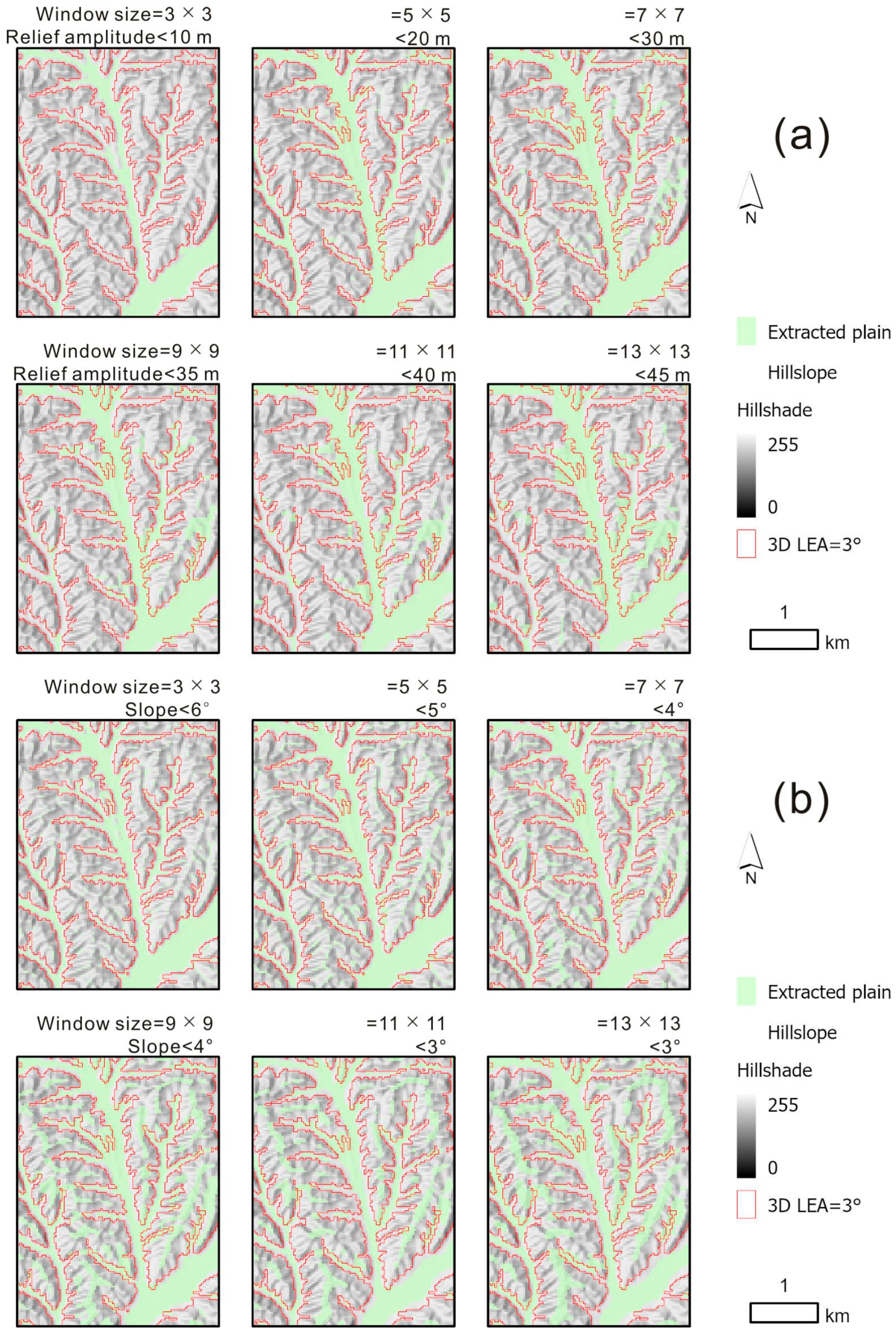
Given the results of previous studies, it was estimated that the area of the intervalley plain was approximately 28%. We can roughly determine the critical values of relief amplitude and slope at different scales by using the 28% low-value area as the intervalley plain. The critical values for relief amplitude can be obtained as 5–10 m, 15–20 m, 25–30 m, 30–35 m, 35–40 m, and 40–45 m for window sizes of 3 × 3, 5 × 5, 7 × 7, 9 × 9, 11 × 11, and 13 × 13, respectively. To prevent plains from appearing on hillslopes, relatively small critical values such as 5 m, 15 m, 25 m, 30 m, 35 m, and 40 m are preferable. Figure 10a shows that, regardless of how large the window size is set, a critical value always extracts a larger plain on the hillslope. Because the total area of the intervalley plain remains constant, excessive extraction of pseudo plains on hillslopes can lead to an underestimation of the true intervalley plain area. The same method can estimate the critical values of multiscale slopes as 5–6°, 4–5°, 3–4°, 3–4°, 2–3°, and 2–3°. Figure 10b shows the slope distribution of sample area 1. To reduce the amount of flat land on the hillside, a relatively small critical slope should be set; thus, we are setting it at 5°, 4°, 3°, 3°, 2°, and 2°. Regardless of how the analysis size changes, there are always low slope values on the hillslope, which are regarded as plains. The 3D LEA = 3° line shows the boundary of the intervalley plain, which is also shown in Figure 10. The figure shows that the relief amplitude and slope are not as good as those of the 3D LEA at many different scales for sample area 1 because of the extraction of pseudoplains within mountain/hillslopes.

Figure 11a shows the relief-amplitude distribution in sample area 2. To increase the area of the intervalley plains, a relatively large critical relief amplitude should be set; thus, we are setting it at 10 m, 20 m, 30 m, 35 m, 40 m, and 45 m. When the window size exceeds 7 × 7, the area below 30 m is very small. The plain extracted by relief amplitude is narrower than the actual distribution pattern of the intervalley plain; otherwise, many pseudo plains are distributed on the hillside. Figure 11b shows the slope distribution for various scales. To better estimate the valley plain by considering low slope values, we set relatively high slope values of 6°, 5°, 4°, 4°, 3°, and 3°. A slope below the critical value is inconsistent with the actual distribution pattern of the intervalley plain, and many pseudo plains are distributed on the hillside. The relief amplitude and slope are unable to distinguish intervalley plains from intermountain flats at many different scales.

In recent years, many studies have carried out automatic landform mapping, with more focus on the selection of mapping models instead of terrain factors [36,37,38,39]. Plains are geomorphic objects that often need to be represented in geomorphic mapping. Slope and relief amplitude are terrain factors that are usually used for landform mapping. The expression of the 3D LEA in the intervalley plain is significantly better than that of the slope and relief amplitude. As mentioned in the text, the slope approaches zero at the maximum elevation position, which usually occurs at the ridge position. On the other hand, the slope is also affected by small fluctuations on the boundary of the intervalley plain, resulting in relatively large values. This new terrain factor 3D LEA is expected to be introduced in future landform mapping. The 3D LEA differs from the previous proposal of 3D MEA [40], which eliminates flat terrain within negative terrain through macroscopic terrain features.

6. Conclusions

This study focused on the limitations of slope and relief amplitude to describe the difference between intervalley plains and intermountain flats. A computer-sight model was built to calculate a novel terrain factor, 3D LEA, to determine the difference. Lanzhou and the surrounding area was used as a case study for the Loess Plateau, where the spatial distribution of intervalley plains is highly important for estimating land resources for urban development. The effects of sight parameters, including the number of directions, look distance, and skip radius, were studied.

The results show that when there are relatively few observation directions, the area of the intervalley plain will be overestimated, so sufficient observation directions are needed. It is recommended to have 12 directions. For 3D LEA to express global terrain features, a sufficient look distance is needed, and it is recommended that this distance exceeds 1000 m. The skip radius can filter small-scale local changes and control the 3D LEA threshold for the intervalley plain. The larger the skip radius, the smaller the critical value. When the skip radius is five grids, the critical 3D LEA should be set to 3°. Furthermore, the function of the sight parameters was explained mathematically on the terrain profile. Additionally, 3D LEA better distinguishes intervalley plains from intermountain flats than do relief amplitude and slope in various analysis windows because the pseudo plains in the mountains are identified by the latter two factors, which leads to an underestimation of the intervalley plains.

The test parameters should vary for different landforms, and additional experimental research is needed. The 3D LEA-based method tends to identify the lowest point on the valley bottom, and this method poorly extracts high terraces in valleys. Although the skip radius can filter out channels with less significant cuts, it does not perform well for channels with particularly significant cuts. However, further research is needed on the impact of intervalley terraces and on targeted-extraction optimization. Future research should focus on the difference between the intervalley plain and upper flat of the lower and wider tablelands. When the look distance reaches a certain value, the area of the pseudo plain does not decrease because the 3D LEA of the upper flat would be lower than the critical value for intervalley plains.

References

- Xiong, L.; Li, S.; Tang, G.; Strobl, J. Geomorphometry and terrain analysis: Data, methods, platforms and applications. Earth-Sci. Rev. 2022, 233, 104191. [Google Scholar] [CrossRef]
- Zhu, M.; Li, F. Influence of slope classification on slope spectrum. Sci. Surv. Mapp. 2009, 34, 165–167. [Google Scholar]
- Chen, W.; Zhou, C.; Chai, H.; Zhao, S.; Li, B. Quantitative extraction and analysis of basic morphological types of land geomorphology in China. J. Geo-Inf. Sci. 2009, 11, 725–736. [Google Scholar]
- Han, H.; Wang, Y.; Li, J.; Gao, T. Classification of Tibetan Plateau Landform Using SRTM-DEM. Remote Sens. Inf. 2015, 30, 43–48. [Google Scholar]
- Hu, Z.; Nie, Y. DEM-Based Landform Taxonomic Features of Hunan Province. Geogr. Geo-Inf. Sci. 2015, 31, 67–71. [Google Scholar]
- Sun, H.; Tang, L.; Yang, S.; Liu, Q. Geomorphology Classification of Anhui Province Based on Digital Elevation Model in Shuttle Radar Topography Mission Data Format. J. Water Resour. Archit. Eng. 2016, 14, 189–192. [Google Scholar]
- Zeng, C. Classification and Regionalization of Geomorphological Types Based on Typical Terrain Indicators and Landform Unit for Sichuan Province, China. Mt. Res. 2021, 39, 587–599. [Google Scholar]
- Wood, J. The Geomorphological Characterization of Digital Elevation Models. Ph.D. Thesis, University of Leicester, Leicester, UK, 1996. [Google Scholar]
- Ehsani, A.H.; Quiel, F. Geomorphometric feature analysis using morphometric parameterization and artificial neural networks. Geomorphology 2008, 99, 1–12. [Google Scholar] [CrossRef]
- Yan, G.; Liang, S.; Ke, Y.; Liu, S.; Zhao, H.; Yang, Z. Optimizing classification of landform element using feature space: A case study in a loess area. Electron. J. Geotech. Eng. 2016, 21, 5814–5824. [Google Scholar]
- Jasiewicz, J.; Stepinski, T.F. Geomorphons—A pattern recognition approach to classification and mapping of landforms. Geomorphology 2013, 182, 147–156. [Google Scholar] [CrossRef]
- Libohova, Z.; Winzeler, H.E.; Lee, B.; Schoeneberger, P.J.; Datta, J.; Owens, P.R. Geomorphons: Landform and property predictions in a glacial moraine in Indiana landscapes. Catena 2016, 142, 66–76. [Google Scholar] [CrossRef]
- Kramm, T.; Hoffmeister, D.; Curdt, C.; Maleki, S.; Khormali, F.; Kehl, M. Accuracy assessment of landform classification approaches on different spatial scales for the Iranian loess plateau. ISPRS Int. J. Geo-Inf. 2017, 6, 366. [Google Scholar] [CrossRef]
- Kang, X.; Wang, Y.; Qin, C.; Chen, W.; Zhao, S.; Zhu, A.; Zhang, S. A new method of landform element classification based on multi-scale morphology. Geogr. Res. 2016, 35, 1637–1646. [Google Scholar]
- Jiang, L.; Ling, D.; Zhao, M.; Wang, C.; Zeng, W. Object-oriented Terrain Position Classification Based on Multi-scale Geomorphons. J. Geo-Inf. Sci. 2018, 20, 281–290. [Google Scholar]
- Stefano, M.D.; Mayer, L.A. An automatic procedure for the quantitative characterization of submarine bedforms. Geosciences 2018, 8, 28. [Google Scholar] [CrossRef]
- Luo, W.; Liu, C.C. Innovative landslide susceptibility mapping supported by geomorphon and geographical detector methods. Landslides 2018, 15, 465–474. [Google Scholar] [CrossRef]
- Chea, H.; Sharma, M. Residential segregation in hillside areas of Seoul, South Korea: A novel approach of geomorphons classification. Appl. Geogr. 2019, 108, 9–21. [Google Scholar] [CrossRef]
- Flynn, T.; Rozanov, A.; de Clercq, W.; Warr, B.; Clarke, C. Semi-automatic disaggregation of a national resource inventory into a farm-scale soil depth class map. Geoderma 2019, 337, 1136–1145. [Google Scholar] [CrossRef]
- Cui, X.; Xing, Z.; Yang, F.; Fan, M.; Ma, Y.; Sun, Y. A method for multibeam seafloor terrain classification based on self-adaptive geographic classification unit. Appl. Acoust. 2020, 157, 107029. [Google Scholar] [CrossRef]
- Tang, G.; Xiao, C.; Jia, D.; Yang, X. DEM based investigation of loess shoulder-line. Geospat. Inf. Sci. 2007, 6753, 67532E. [Google Scholar]
- Yang, X.; Li, M.; Na, J.; Liu, K. Gully boundary extraction based on multidirectional hill-shading from high-resolution DEMs. Trans. GIS 2017, 21, 1204–1216. [Google Scholar] [CrossRef]
- Dai, W.; Yang, X.; Na, J.; Li, J.; Brus, D.; Xiong, L.; Tang, G.; Huang, X. Effects of DEM resolution on the accuracy of gully maps in loess hilly areas. Catena 2019, 177, 114–125. [Google Scholar] [CrossRef]
- Wei, H.; Xiong, L.; Zhao, F.; Tang, G.; Lane, S.N. Large-scale spatial variability in loess landforms and their evolution, Luohe River Basin, Chinese Loess Plateau. Geomorphology 2022, 415, 108407. [Google Scholar] [CrossRef]
- Yuan, S.; Xu, Q.; Zhao, K.; Wang, X.; Zhou, Q.; Chen, W.; Pu, C.; Li, H.; Kou, P. Loess tableland geomorphic classification criteria and evolutionary pattern using multiple geomorphic parameters. Catena 2022, 217, 106493. [Google Scholar] [CrossRef]
- Hawker, L.; Uhe, P.; Paulo, L.; Sosa, J.; Savage, J.; Sampson, C.; Neal, J. A 30 m global map of elevation with forests and buildings removed. Environ. Res. Lett. 2022, 17, 024016. [Google Scholar] [CrossRef]
- Travis, M.R.; Elsner, G.H.; Iverson, W.D.; Johnson, C.G. VIEWIT: Computation of Seen Areas, Slope and Aspect for Land-Use Planning; USDA Forest Service General Technical Report PSW-1V1975; Department of Agriculture, Forest Service, Pacific Southwest Forest and Range Experiment Station: Albany, CA, USA, 1975.
- Deng, J.; Cheng, W.; Liu, Q.; Jiao, Y.; Liu, J. Morphological differentiation characteristics and classification criteria of lunar surface relief amplitude. Acta Geodartica Cartogr. Sin. 2022, 77, 1794–1807. [Google Scholar] [CrossRef]
- Liang, H.; Zhao, S.; Ma, D. ALOS DEM-Based Extraction of geomorphological feature in Xishan mining area of Shanxi Province. J. Taiyuan Univ. Technol. 2022, 54, 950–958. [Google Scholar]
- Yokoyama, R.; Shlrasawa, M.; Pike, R.J. Visualizing Topography by Openness: A New Application of Image Processing to Digital Elevation Models. Photogramm. Eng. Remote Sens. 2002, 68, 257–265. [Google Scholar]
- Mark, R.K. Multidirectional, Oblique-Weighted, Shaded-Relief Image of the Island of Hawaii; US Geological Survey Open-File Report; US Department of the Interior, US Geological Survey: Reston, VA, USA, 1992; pp. 92–422.
- Smith, M.J.; Clark, C.D. Methods for the visualisation of digital elevation models for landform mapping. Earth Surf. Process. Landf. 2005, 30, 885–900. [Google Scholar] [CrossRef]
- Hiller, J.K.; Smith, M. Residual relief separation: Digital elevation model enhancement for geomorphological mapping. Earth Surf. Process. Landf. 2008, 33, 2266–2276. [Google Scholar] [CrossRef]
- Prima, O.D.A.; Echigo, A.; Yokoyama, R.; Yoshida, T. Supervised landform classification of Northeast Honshu from DEM-derived thematic maps. Geomorphology 2006, 78, 373–386. [Google Scholar] [CrossRef]
- Yan, G.; Cheng, H.; Jiang, Z.; Teng, L.; Tang, M.; Shi, T.; Jiang, Y.; Yang, G.; Zhou, Q. Recognition of fluvial bank erosion along the main stream of the Yangtze River. Engineering 2022, 19, 50–61. [Google Scholar] [CrossRef]
- Iwahashi, J.; Pike, R.J. Automated classifications of topography from DEMs by an unsupervised nested-means algorithm and a three-part geometric signature. Geomorphology 2007, 86, 409–440. [Google Scholar] [CrossRef]
- Drăguţ, L.; Eisank, C. Automated object-based classification of topography from SRTM data. Geomorphology 2012, 141–142, 21–33. [Google Scholar] [CrossRef]
- Iwahashi, J.; Kamiya, I.; Matsuoka, M.; Yamazaki, D. Global terrain classification using 280 m DEMs: Segmentation, clustering, and reclassification. Prog. Earth Planet. Sci. 2018, 5, 1. [Google Scholar] [CrossRef]
- Du, L.; You, X.; Li, K.; Meng, L.; Cheng, G.; Xiong, L.; Wang, G. Multi-modal deep learning for landform recognition. ISPRS J. Photogramm. Remote Sens. 2019, 158, 63–75. [Google Scholar] [CrossRef]
- Yan, G.; Tang, G.; Chen, J.; Li, F.; Yang, X.; Xiong, L.; Lu, D. Modeling computer sight based on DEM data to detect terrain breaks caused by gully erosion on the loess Plateau. Catena 2024, 237, 107837. [Google Scholar] [CrossRef]