What Local Environments Drive Opportunities for Social Events? A New Approach Based on Bayesian Modeling in Dallas, Texas, USA

Abstract

In-person social events bring people to places, while people and places influence where and what social events occur. Knowing what people do and where they build social relationships gives insights into the distribution and availability of places for social functions. We developed a Bayesian Network model, integrating points of interest (POIs) and sociodemographic characteristics, to estimate the probabilistic effects of places and people on the presence of social events. A case study in Dallas demonstrated the utility and performance of the model. The Bayesian Network model predicted the presence likelihoods for seven types of social events with an R² value around 0.83 (95% confidence interval). For both the presence and absence of social events at locations, the model predictions were within a 20% error for most event types. Furthermore, the model suggested POI, age, education, and population density configurations as important contextual variables for place–event associations across locations. A spatial cluster analysis identified likely multifunctional hotspots for social events (i.e., socially vibrant places). While psychological and cultural factors likely contribute further to local likelihoods of social event occurrences, the proposed conceptually informed geospatial data-science approach elucidated intricate place–people–event relationships and implicates inclusive, participatory places for urban development.

1. Introduction

Social events provide participatory opportunities that make human connections, cultivate social capital, and shape the social fabric of a community [1,2]. In this study, we consider places with social events as locales, where material context and settings meet the functional and operational needs of the correspondent social events. Locales bring people together across space at a particular time and serve as spatial catalysts for human dynamics.

Geospatial studies on human dynamics commonly adopt a Time Geography framework to model individuals’ movements as “space-time paths” and estimate accessibility and interaction opportunities subject to the constraints of capabilities, couplings, and authority structures [3]. Some research on human mobility patterns examines the regularities of movements between activity sites [4,5]. While these studies have yielded valuable insights into the rhythms, patterns, and purposes of movements, they consider locales as nodes in movement trajectories without attention to social events taking place there. Urban design promotes human interactions through pedestrian access, for example, and venues provide gathering places to facilitate in-person meetings [6]. While extensive research uses sociometric data to analyze social ties and positions in human relationships (e.g., kinships or friendships) and social networks [7], few studies consider social events that bring people to a specific physical space and how and what social events may effectively promote positive human relationships [8]. There are community-focused locales, such as a diner, with a proper material context to support gatherings of friends and families. There are also legendary locales equipped with multifunctional physical settings attract diverse social events and people. The Sydney Opera House, for example, hosts a wide range of cultural and social events, including concerts, festivals, and talks, attracting people from around the world. Locales individually support and are supported by people and their social activities and, furthermore, collectively characterize the communities where the locales operate.

This study aims to understand the spatial probabilities of locales for different social event types given various places and populations in a city. Locales are places where social events occur because these places provide the material context or physical settings capable of supporting the social events happening there. We assumed the existence of associations between places, people, and social events. Moreover, we assumed convergent attraction from proximate places (micro-locales) that together form a meso-locale with complementary affordances to support multiple social events (for example, a parent meeting and a play day at a coffee shop next to a children’s fun center). We expected that Bayesian inference with conditional probabilities could capture the place–people–event association more effectively than linear and logistic regression (LR), spatial autoregressive regression (SAR), and conditional autoregressive regression (CAR) because the place–people–event association and the convergent attraction would dwarf LR, SAR, and CAR interpolations of the probability of event occurrences based merely on spatial distributions of events. Furthermore, Bayesian Network modeling combines a graph structure and probabilities among variables to examine causal relationships on the ground that causal variables can increase the probabilities of their effects. In other words, if C is a causal factor to affect E, then the conditional probability P(E|C) shall be greater than the probability P(E) with the acknowledgment that we may not know all the causes and not all causes are equally important [9].

As such, we developed a Bayesian Network Model and tested the model using data from the 63-mile area around the city of Dallas in the U.S. The model predicted the spatial probabilities for each social event type based on variables for places and people. The social event type with higher prediction accuracy suggests a stronger spatial association of place types, people, and social event types and, hence, stronger locales. Furthermore, we applied local spatial autocorrelation statistics to identify macro-locales of clusters with high probabilities of social event types, place types, and characterized populations. We perturbed the input data with multiple spatial shifts to mitigate zoning effects on spatial clustering. The next section highlights recent geospatial studies on events to clarify the novel aims, conceptual framework, and proposed approach to geospatial modeling of social events in this research. The sections that follow detail the data, methods, findings, discussions, and conclusion of the study.

2. Geospatial Studies of Events, Places, and People

Social events are dispersed socially and geographically and are difficult to collect. While there are many databases that characterize places and people, to the best of our knowledge, there are no data sets systematically recording where and what ordinary people do. The rise in ambient geospatial big data has stimulated many novel approaches to identifying geospatial events and performing large-scale geospatial modeling. Moreover, geospatial research shifts foci from attributes, features, and fields to events, movements, and dynamics. Most of these geospatial events are public events, such as infections, hazards, festivals, political rallies, or hate speeches. Analytical emphases of these events center on the event patterns in space and time for the predictions of changes in event locations or spatial distributions over time. Our study differs from these studies by focusing on social events organized by ordinary people and the spatial associations of place, people, and social events. Despite the differences, the overview below highlights the conventional approaches to geospatial event modeling in contrast to this research.

Social sensing data, such as geo-tagged social media posts and Call Detail Records from smartphones, are popular sources for mining geospatial events. Studies on event extraction from social media data and ensuing analysis of these extracted events commonly apply some combinations of methods from natural language processing, regression modeling, semantic patterns, or machine learning. Xiang and Wang [10] detailed the tasks, methods, and algorithmic progress in the field. Geospatial event extraction follows the general workflow with added considerations of the spatial dimension.

For example, Gao et al. [11] used a bag-of-words model and support vector machine (SVM) algorithm with keyword filtering to classify tweets as event-related or event-unrelated. Then, they applied kernel density estimation (KDE) to model the surface of the rates of event-related posts to the total posts within individual spatial units for each period. These temporal surfaces represented spatial event prevalence and served as the basis to determine statistical p-values for anomalous event patterns, such as influenza activities. Beyond identifying anomalies in spatial event patterns over time, researchers applied semantic analysis to examine the content of posts to model the topical clusters among the posts and, furthermore, how these topics are distributed and correlated over space. Xu, Li, and Huang [12] detected irregular busts of tweets as candidates for local events during the Toronto International Film Festival (TIFF) and spatially aggregated clusters of similar topics with various thresholds that led to an estimate of 673 local events, among which 86 TIFF events and 498 non-TIFF events were correctly identified.

The idea that sudden changes in space and time signal event occurrences thrives with the proliferation of human mobility data from smart cities and location-aware sensing technologies, including GPS-equipped vehicles, transit smartcards, smart phones and watches, and various geo-tagged user-generated content (such as tweets, four-square check-ins, or customer reviews). These multimodal data of high density in space and time characterize human dynamics in a city and subserve the detection of anomalies that signal disruptive events, such as concerts or accidents that cause traffic jams. Jayarajah et al. [13] showed that events from anomaly detection from such multimodal data accounted for 30–50% of published events (e.g., concerts) within 1.5 km of the event venues or up to 80% within 4 km in Singapore and New York City. Relating mobility data to land use, Widhalm et al. [14] reconstructed trips, visited places, and clusters of home, work, shopping, and leisure activities in Vienna and Boston.

Research on how events relate to places and people commonly uses case studies of mega or hallmark events, such as Arts Festivals [15,16], Olympic Games [17,18,19], World Fairs, and Expositions, to investigate social, economic, and cultural impacts on the local communities. Yet, cultural festivals, such as The Notting Hill Carnival in London, have significant contributions to local cohesion. Despite their ephemerality, the intensity of social interactions at such festivals can foster a strong sense of belonging, particularly among younger community members and festival-goers, enhancing the social fabric of urban spaces [20].

Large-scale geospatial analysis of events, places, and people is scarce, but the two examples below suggest a rich ground for geographic knowledge. Calabrese et al. [21] used one million call detail records to show the origins of people attending events from 30 July to 12 September 2009 in Boston and 15 large-scale events from Boston Global news online. Under many caveats, the research suggests that what events people attend are strongly correlated with where people live (e.g., the closer, the more likely) and the type of events (e.g., people show event preferences). Currid and Williams [22] used Getty Images of 300,000 geotagged photos taken at 6000 arts and entertainment events from March 2006 to March 2007 in Los Angeles and New York City to analyze macro-geographic patterns of social milieus by identifying event enclaves and cultural hubs. Their study concluded two types of event locations: “overly frequented locations hosting multiple social events” and “places where major events were held annually or semi-annually” (p. 436). These popular event venues serve vital functions for place branding.

Places are pivotal to event making and human interactions. For example, urban design builds pedestrian access to promote human interactions and create venues to facilitate in-person meetings [6]. Hawker Center in Singapore serves not just as a dining place but as a vibrant community hub that promotes social connectedness and well-being [23]. These spaces become integral to community resilience, especially during stressful events like the COVID-19 pandemic, by maintaining a sense of normalcy and encouraging responsible behaviors. The design of public spaces, such as streets, can foster social encounters [24].

While the cited studies above are limited, their extensive references in literature reviews suggest similar tracks of inquiries and methodologies. Geospatial research on events is intensive, but most studies focus on one event type, one case, one place type, or one kind of relationship. In contrast, our study aims to seek spatial associations among multiple types of events, places, and people, and with the spatial associations, it aims to predict the likelihood of each event type to occur at a place type and the characteristics of the population residing around the place.

3. Data

Comprehensive data for social events and places of the event venues are dispersed across physical and digital media, such as classified posts in local newspapers, posters in public libraries and community centers, and announcements in various social media outlets (e.g., Facebook, X, Nextdoor, LinkedIn, and Google Event Calendar). As our emphasis is on community-based events, Meetup.com (henceforth, simply Meetup) captures a wide variety of social events from people who share common interests in communities nearby and brings online communities offline. Meetup has over 58 million members and 20 years of social events catering to diverse interests and hobbies. Studies showed that social events at Meetup enhanced attendees’ engagement and created bonded social capital [25], reflected the economically advantaged geographies associated with regional median income with the type of meeting venues and activities [26], and served alternative measures for entrepreneurial ecosystems [27,28]. The latest Meetup report (https://www.meetup.com/marketing-assets/PDF/Meetup+Trend+Report+v13.pdf, accessed on 21 October 2023) showed shifts in popular event types from technology and processional-focused events in 2019 to authentic friendships (including Queer and LGBTQ) in 2022. Meetup does not collect demographic data. However, web traffic analytics by similarweb.com (https://www.similarweb.com/website/meetup.com/#demographics, accessed on 21 October 2023) showed 49% female and 51% males among the 18.3 million site visits in September 2023, and approximately one-third (33.77%) of the visits from the age group 25–34 and reasonable spread across other age groups (12.75% 18–24, 19.72% 35–44, 16.31% 45–54, 11.32% 55–64, and 6.13% 65+).

For places of event venues, we choose Points of Interest (POI) data from SafeGraph.com (henceforth, simply SafeGraph). POIs traditionally represent visually and culturally important features on maps. The rise of digital maps and microeconomic interest popularizes the POIs with business establishments and tourist landmarks in cities. In this context, many POIs serve as third places complementary to home (the first place) and work (the second place) and become an essential part of many people’s daily lives. As such, POIs give meanings to locations and can be referred to as places [29]. When the meaning of POIs comes from social events that have produced shared experiences and memories, the POIs are not only places but micro-locales. Many POI data solicitors and providers exist, such as Google Places, OpenStreetMap, Yelp, Four Square, ArcGIS, and Maptitude. Our choice of SafeGraph POI dataset is due to three main reasons: (1) detailed technical documentation (https://docs.safegraph.com/docs/places, accessed on 21 October 2023) on data collection, processing, metadata, and accuracy assessment; (2) free access for academic research and used in 2000+ published studies; and (3) global coverage and routine updates and maintenance. The first reason asserts confidence in data quality. The other two reasons enable our proposed methods and research findings to be compared and contextualized in the literature, allowing for reproducibility and replicability beyond the study site.

Specifically, we used “DFW, TX” to retrieve events at Meetup from 26 February 2020 to 30 January 2021, a period of reduced social activities amid the COVID-19 pandemic. Meetup adopted GraphQL to handle data requests. On spatial queries, GraphQL requires longitudes and latitudes instead of city names and uses Geonames (http://www.geonames.org, accessed on 21 October 2023) as the default geocoder. The input “DFW, TX” was converted to us-tx-dfw to check Geonames entries. The matched city was Dallas, so Geonames returned the latitude and longitude coordinates (N 32°46′59″ and W 96°48′24″). Returned events were within 63 miles of the query center, so we set a 63-mile radius as the study area boundary. By removing online events and those lacking geographic coordinates, we retained 9445 social events across 1537 unique locations. These in-person social events took place during the COVID-19 pandemic, when many people opted to reduce human contact, signaling the robust nature of social gatherings and the social importance of micro-locales.

The Meetup platform categorized these events into 24 distinct categories, and we subsequently grouped the categories into seven (7) event types (

Table 1. Categories of social events from Meetup.

Reclassified Category	Original Category	Reclassified Category	Original Category
Movements (no similar events to merge up but instance is enough to be an isolate type, same for Career and Business)	Movements (e.g., women’s opportunity movements, decolonial movements)	Religion and Identity	Beliefs
Science and Education	Tech		LGBTQ
	Learning	Career and Business	Career and Business
	Writing	Sports and Health	Health and Wellness
	Book Clubs		Sports and Fitness
Hobbies and Passions	Sci-Fi and Games		Outdoors and Adventure
	Dance	Social Activities	Social
	Music		Language and Culture
	Food and Drink		Pets
	Hobbies and Crafts		Family
	Arts
	Photography
	Film
	Fashion and Beauty

) for a helpful heuristic in information processing. However, recent publications argued for even lower cognitive limits [30,31]. Many POIs are closely located to each other and quickly blur point distributions. We aggregated POIs by hexagons with an edge length of 2000 m to visualize the spatial distributions of POI types (Figure 1A). All seven social event types were commonly held in central Dallas, with trends towards the north and the southwest. A vast peripheral area had no posted social events at Meetup, which could indicate biases towards urban centers and spatially extensive POIs, like parks where all events would be geo-coded to their centroids. Sports and Health and Hobby and Passion were the most popular and widely held across the metroplex. In contrast, Movement events were most concentrated in residential areas, primarily due to their focus on community service and charitable activities. The widely distributed Hobby and Passion event type is attributed to its diverse activities across various populations. In contrast, the Movement event type is specific to social and political movements and, hence, often takes place at locations of social or political significance. Figure 2 shows word clouds from Meetup posts for the two event types to highlight event compositions in the two categories. The other four event types, Social Activities, Science and Education, Region and Identity, and Career and Business, were distributed comparably over space.

An event post on Meetup included the organizer, event description, location (POI and addresses), date and time, and attendees. Figure 1B shows an example of Hobbies and Passions: a drawing event from 7:30 to 9:30 p.m. on Wednesday, 4 March 2020, at Flagship Half Price Books, 5803 East Northwest Highway, Dallas. The event was for the Dallas Sketchers group but was also open to the public.

Similarly, we downloaded all POI data in March 2020 from SafeGraph and selected 102,920 POIs with North American Industry Classification Systems (NAICS) categories (

Table 2. SafeGraph POI categories and frequencies in the Study Area.

Category	# POIs	Category	# POIs
Retail Trade	26,181	Arts, Entertainment, and Recreation	5351
Health Care and Social Assistance	18,479	Educational Services	3709
Other Services (except Public Administration)	17,657	Real Estate and Rental and Leasing	2830
Accommodation and Food Services	16,825	Professional, Scientific, and Technical Services	1947
Finance and Insurance	7698	Information	1426
Public Administration	866	Transportation and Warehousing	1319
Wholesale Trade	743	Administrative and Support and Waste Management and Remediation Services	1058
Construction	189	Manufacturing	917
Utilities	116	Management of Companies and Enterprises	8
Agriculture, Forestry, Fishing and Hunting	9

) within the study area. To spatially relate social events and POIs, we tessellated the study area into a grid of hexagons with an edge length of 400 m, representing a common walkable distance [32,33]. In the subsequent spatial clustering analysis, hexagons were chosen over squares for their isotropic spatial relations to their neighbors and ensuing advantages. This study only considered those hexagons within 400 m from any POIs, which includes hexagons with POIs or within 400 m from any POI (Figure 3), because we intended to model the spatial probabilities of locales of different social event types given various places (i.e., POI types). Hexagons without POIs but within 400 m of any POI are considered reachable by foot, so social events in these hexagons could be associated with these POIs outside the hexagons. For simplicity, we subsequently used POI-hexagons to include both hexagons with POIs and hexagons within 400 m of any POI. Of the 9445 social events in this study, 9361 (or 99%) occurred in POI-hexagons. The remaining 1% of events predominantly comprised sports activities in lakes or parks with spatial extent far beyond the POI label points or private venues without POI designations. Therefore, hexagons without POI or beyond 400 m of any POI (i.e., not POI-hexagons) were removed from the study.

4. Methods

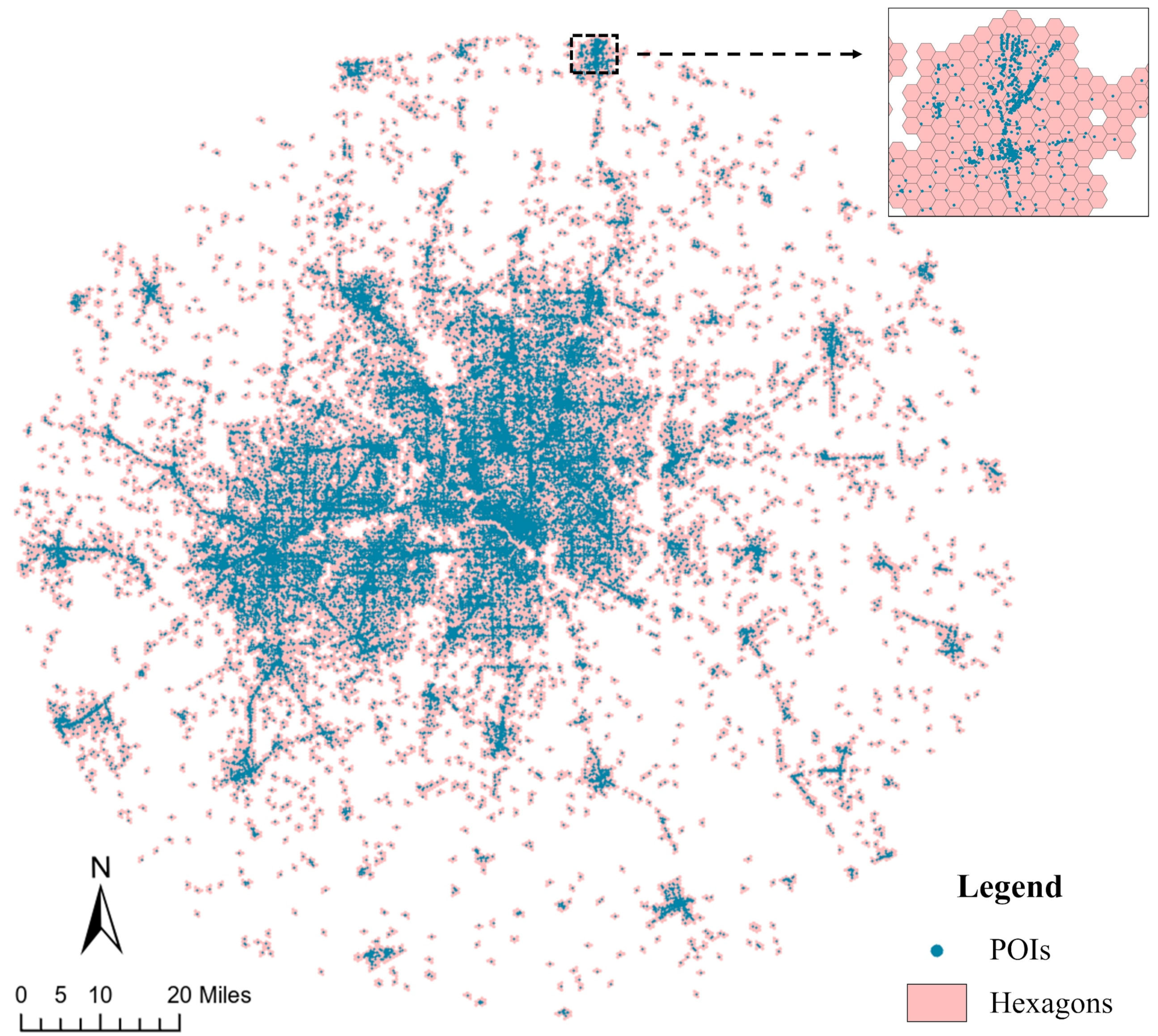
Each POI-hexagon served as a unit of analysis in our study to spatially associate places, people, and social event types. We developed a Bayesian Network model to explicitly compute the conditional probability of event occurrences, given the probabilities of sociodemographic quantities within a POI-hexagon and the POIs within 400 m of the POI-hexagon’s boundary. We then compared the Bayesian model with other conventional methods to affirm the advantages of Bayesian Network modeling.

We chose Bayesian Networks (BN), developed by Pearl [34] and also known as belief networks or Bayes nets, to model probabilistic relationships among places, people, and social events for three reasons. First, popular machine learning methods, such as Random Forests (RF), Support Vector Machines (SVM), and Neural Networks (NN), despite their predictive power, are characterized by their black-box operations and limited interpretability to relate input variables to the output variable [35]. BN can model multiple non-mutually exclusive distributions of predictive variables, but discriminative classifiers, like RF or SVM, are subject to the predicted probabilities summed to 100% [36]. Second, generalized linear regression and its spatial extensions, such as spatial autoregressive (SAR) and conditional autoregressive (CAR) models, assume predefined relationships among variables and therefore lack the flexibility to model complex associations. BN, in contrast, requires no predefined rigid functional forms [37]. The third reason is BN’s ability to maximize posterior queries to determine the most probable network configuration based on the learned joint distributions for a given observation.

4.1. Probability Modeling

BN modeling depends heavily on the underlying graphical structure that should align with the corresponding domain knowledge. In a graphical structure, nodes symbolize variables, and edges represent conditional dependencies between them. Network dependencies learned by data-driven approaches may sometimes contradict domain knowledge. For instance, in the context of this research, POIs support social events under the research assumption that an event takes place where material context and physical settings can meet the event’s functional needs. Therefore, the BN structure should direct edges from POI types to event types. Nevertheless, data-driven approaches may result in social events as precedents to POI types. While it is possible that a POI was built to host a preplanned event (such as building an arena for an Olympic game), this research is limited to using POIs to predict social events, as our interest is in the implications of what places we have in a community and what people do and relate to in the community.

To examine the validity of this research assumption, POI preceding social events, we calculated the presence rates of social events in POI-hexagons to show the POI effects on event presence. For social events, most POI presences are associated with higher event presence rates (Figure A1). The only exception was with Management and Remediation Services (MgmEnterp) and Agriculture, Forestry, Fishing and Hunting (AgriFish) POI-hexagons. In contrast, the effects of social event types on POI presence are negligible (Figure A2). Subsequently, we adopted the network structure with directed edges from POI types to social event types (Figure 4).

A social event cannot take place without participants. Therefore, population characteristics can affect what kinds of social events are likely to occur in a community. We acquired five-year (2017–2021) estimates of demographic and socioeconomic (henceforth simply sociodemographic) data at the census tract level from American Community Surveys (ACS). The selected ACS variables included population density per square meter; age brackets of under 18, 18–44, 45–64, and over 64 years old; race categories of White, Black, Asian, and Other; educational attainment levels of completing middle school, high school, or college; per capita income; and poverty rates, for a total of 14 sociodemographic variables. We calculated the area-weighted average of each variable in individual POI-hexagons. These sociodemographic variables and POI-type probabilities are input variables to predict the probabilities of social events in every POI-hexagon. Micro-locales would be identified if a particular POI type exhibited robust predictability for a specific social event type. Spatial clusters of POI-hexagons with high probabilities of social event types of interest suggest meso- or macro-locales.

The added sociodemographic variables necessitated the consideration of a condition in which the two variables (POI types and social event types) become dependence-separated (i.e., d-separated) in the BN. Figure 5 gives a d-separated example of a directed path from X₁ to S₁ through X₂. If X₂ is not an empty set, the path X₁ to S₁ is blocked by conditioning on the intermediary X₂; hence, X₁ and S₁ are dependence-separated upon X₂. Structural revisions to the Bayesian network aim to identify sociodemographic variables (X₁) that can mediate previously independent POI types (X₂) to a specific type of social event (S₁) and, therefore, improve the Bayesian network model’s predictability of social events. For illustrative purposes, let us examine the religious sociodemographic variable (e.g., Christianity, Islam, Hinduism) denoted as X₁. These variables are often associated with the presence of specific POIs, represented as X₂, such as churches, mosques, or temples. Consequently, the type of religious events (S₁) can be directly deduced from the type of worship place (POI), obviating the need for additional sociodemographic data in this context. In such instances, X₁ is deemed d-separated from S₁, with the observation of X₂. Conversely, in the absence of POI data, the local sociodemographic variables can still facilitate inferences about likely social events. Under these circumstances, X₁ is d-connected to S₁ in the absence of X₂ observations. An alternative, X₂ to S₁ through X₁, is also possible; some POI types may condition the dependence between sociodemographic variables and social event types. Because all hexagons under consideration have POIs and sociodemographic values (i.e., not empty sets), the proposed Bayesian Network model considered both d-separation alternatives.

BN modeling needs to account for the soundness and completeness of d-separation [38]. Given that all predictors, encompassing both local sociodemographic and POIs, are observable in this study, dependencies among these variables will form d-separation to social events nodes, which will inflate the computational load without improving model performance. Consequently, we constructed a graph with direct edges from all predictors to social events nodes, as the priori assumption in BN. In practice, the validity of these edges was evaluated using mutual information, ensuring the accuracy of the dependency assumptions [39]. This study considered 19 POI types, 14 demographic and sociodemographic variables, and 7 social event types. The conditional probability of presence for a given social event type (S_i) in a POI-hexagon is subject to the probabilities of a given possible state defined by the 33 variables characterizing POI types and sociodemographic conditions:

$$\mathrm{P}({\mathrm{S}}_{\mathrm{i}}={\mathrm{s}}_{\mathrm{i}}|{\mathrm{X}}_1={\mathrm{x}}_1,\dots ,{\mathrm{X}}_{33}={\mathrm{x}}_{33}) \mathrm{for} \mathrm{i} = 1 \mathrm{to} 7$$

(1)

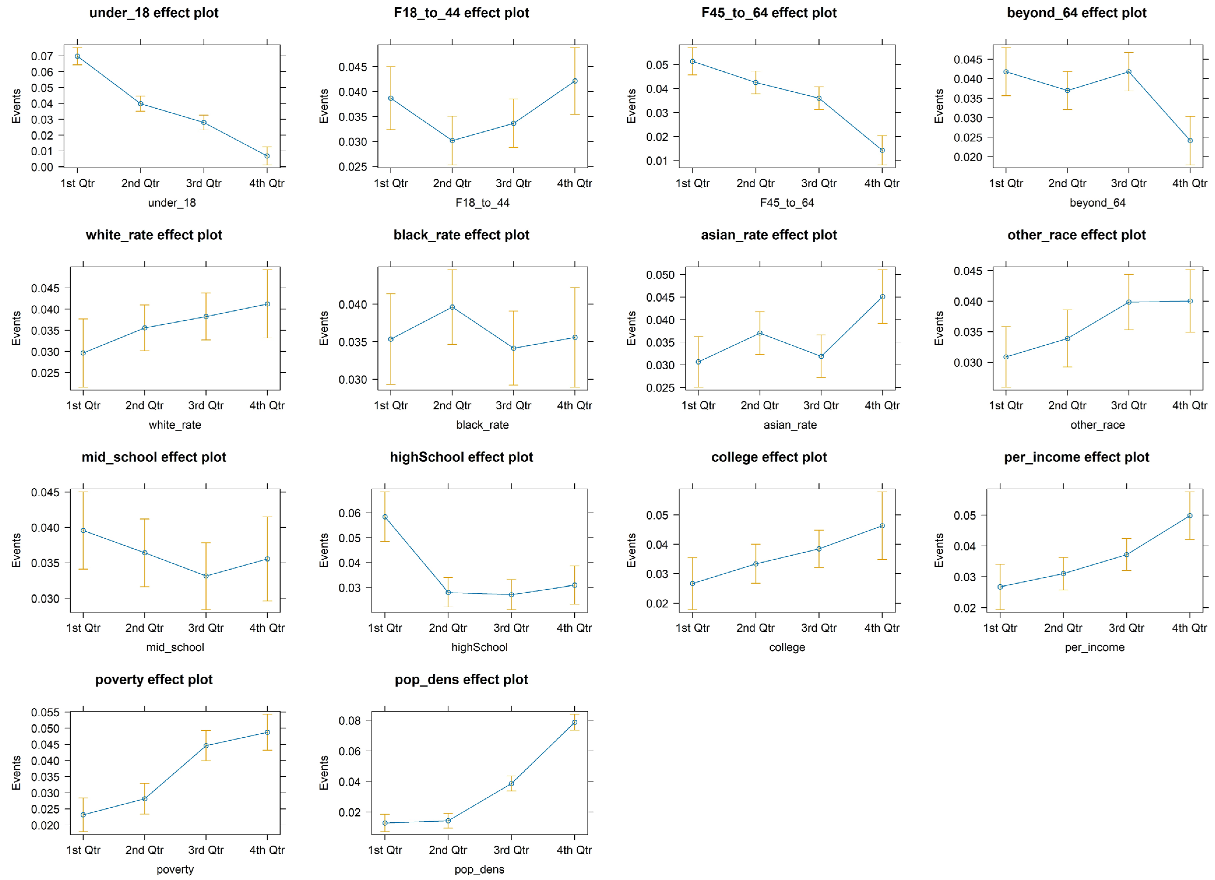
We treated POI types as binary variables to encode their presence (=1) or absence (=0) for each POI-hexagon. Sociodemographic variables were continuous values, and it would be infeasible to consider all possible combinations of unique values. As such, we transformed these sociodemographic data into categorical variables based on the quantile distributions of the respective variables. The percentages of POI-hexagons with social events varied across quantiles in each demographic and socioeconomic variable (see effects plots in Figure A3). Most of these variables as quantiles exhibited negative or positive effects on the presence of social events, albeit with different degrees of uncertainty. For instance, increasing quantiles of residents under 18 decreased the percentage of POI-hexagons with social events from 8% to 1% with high confidence intervals across all four quartiles. The decreasing effects implied that the majority of social events from Meetup in the study area were for adult participants. On the other hand, middle school attainment and the percentage of the Black population showed wide confidence intervals. Therefore, the quantiles of neither variable had robust effects on the presence of social events.

We applied a forward stepwise model selection approach to rank the predictive contributions of all 33 variables (19 POIs and 14 demographic and socioeconomic variables) under linear assumptions. For each iteration, the stepwise model selection added each variable into the model prediction and then compared the model performance with each added variable based on improvements in reducing the residual sum of squares and the Akaike Information Criterion (AIC) measure. While the study considered 33 variables, the results showed increases in the residual sum of square and AIC measures in the 27th iteration (

Table 3. Predictor importance rank by AIC.

Variables	Rank	Resid. Dev	AIC	Variables	Rank	Resid. Dev	AIC
	NA	890.58	−85,757	+ college	13	771.15	−89,410
+ Manufac	1	844.70	−87,106	+ RealEstate	14	770.47	−89,431
+ ProfSvcs	2	822.66	−87,780	+ HealthCare	15	770.04	−89,443
+ highSchool	3	807.71	−88,246	+ pop_dens	16	769.38	−89,463
+ Wholesale	4	798.15	−88,549	+ ArtsRec	17	768.99	−89,474
+ PubAdmin	5	791.17	−88,771	+ poverty	18	768.51	−89,488
+ F18_to_44	6	785.33	−88,959	+ AccomFood	19	768.23	−89,495
+ under_18	7	781.45	−89,083	+ EduSvcs	20	768.00	−89,500
+ Info	8	778.19	−89,188	+ mid_school	21	767.83	−89,504
+ TransWare	9	775.96	−89,259	+ other_race	22	767.73	−89,506
+ Utilities	10	774.00	−89,322	+ black_rate	23	767.65	−89,506
+ Construct	11	772.71	−89,362	+ per_income	24	767.58	−89,506
+ AdminSup	12	771.86	−89,389

).

Improvements to model fit in residuals and AIC decreased as the number of variables increased and became negligible around the 20th rank. For computability, we considered the first 20 variables, 14 POI types, and 6 sociodemographic variables to build a BN model for predicting the probability of the presence of each social event type: a total of seven probabilities for seven event types in a local environment (e.g., a POI-hexagon in the analysis). This resulted in approximately 67 million states for conditional probabilities: $\mathrm{P}\left({\mathrm{S}}_{\mathrm{i}}={\mathrm{s}}_{\mathrm{i}}{|\mathrm{X}}_1={\mathrm{x}}_1,\dots ,{\mathrm{X}}_{20}={\mathrm{x}}_{20}\right) \mathrm{for} \mathrm{i}=1 \mathrm{to} 7$. The final multivariate linear model accounted for 13.0–14.6% (95% confidence interval) of the spatial variance in social events, providing a baseline fit prior to BN modeling.

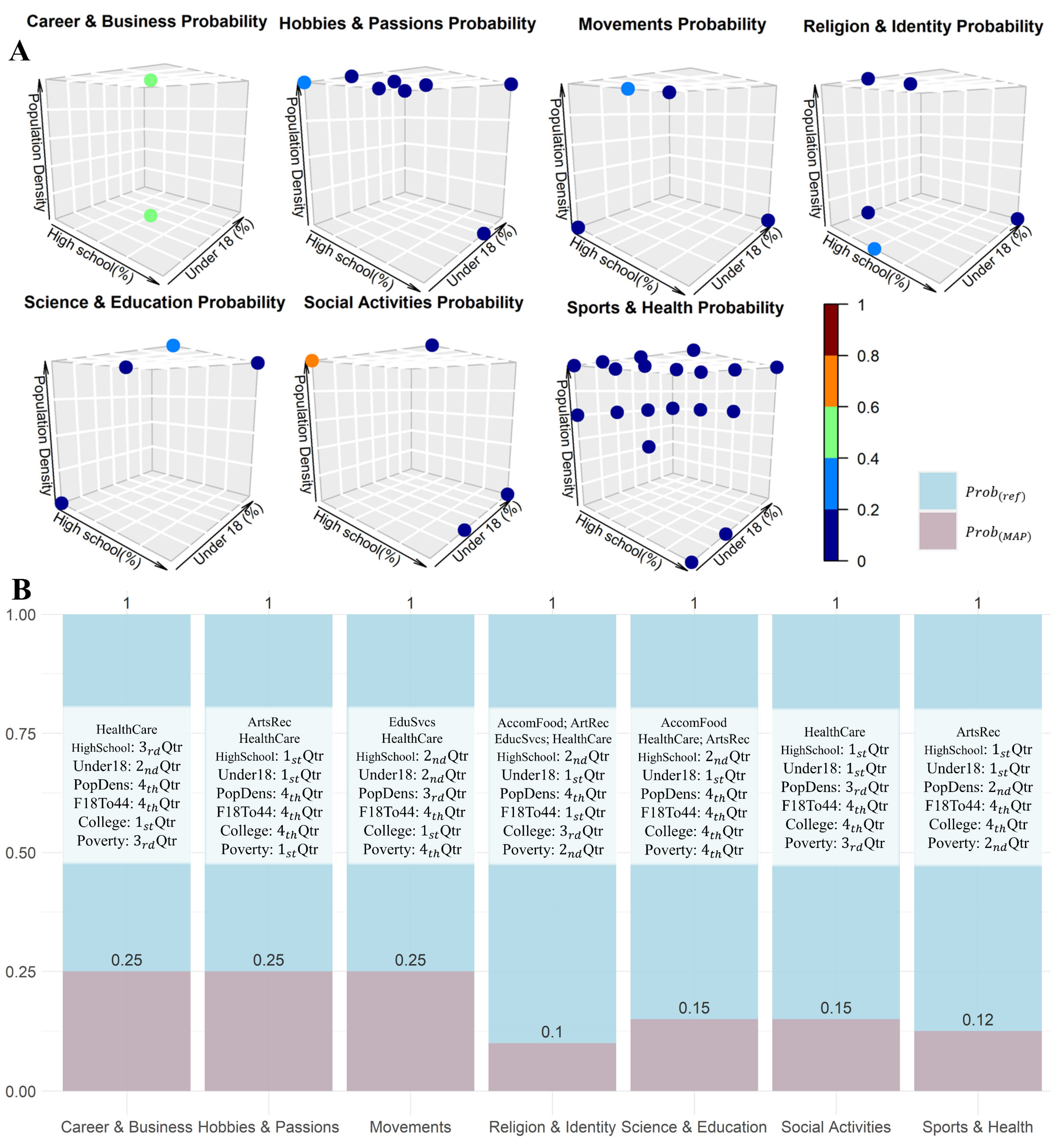
To further explore the influences on social event likelihoods, we applied conditional probability distributions (CPDs), a foundational statistical tool capturing event probabilities under specific conditions. This method models event probabilities in context-specific ways, offering insights into the collective contributions of different combinations of factors to social events [40,41]. Additionally, we utilized the Maximum A Posteriori (MAP) query to identify the most probable combinations of POIs and sociodemographic attributes in areas hosting social events. MAP, rooted in Bayesian statistics, estimates optimal parameter sets from observed data, effectively pinpointing pivotal factors facilitating social events. This approach is especially informative in urban studies, aiding urban planners and policymakers in making informed decisions about community engagement and urban development [42]. These statistical techniques estimated event probability distributions under varying conditions, revealed the critical contextual determinants conducive to social events, and drew valuable insights into POIs as a social infrastructure that can enhance the fabric of urban community life [43].

4.2. Spatial Clustering Analysis

The proposed BN model predicted the presence probability of each social event type in each POI-hexagon based on the assembly of POI types and sociodemographic characteristics for the respective POI-hexagon. As such, each POI-hexagon with social events is a meso-locale, while each POI with a high probability of at least one social event type is a micro-locale. A spatial cluster of POI-hexagons with high probabilities of at least one social event type gives rise to a macro-locale. We applied local spatial autocorrelation statistic (local Moran’s I) to identify significant hotspots representing macro-locales for each social event type. Local Moran’s I measures the similarity between a focal location and its spatial neighbors [44] to quantify the correlation of social event probabilities between the focal hexagon and its adjacent hexagons. Positive values indicate clustering of similar values (high–high or low–low), while negative values suggest marginalized or isolated meso-locales. Getis-Ord Gi* is another common local metric that assesses whether the values of individual neighborhoods differ from the global values in the study area [45]. Local Moran’s I fit better the conceptualization from meso-locales to macro-locales than Getis-Ord Gi*.

Since we tessellated the study area to a hexagon grid and used POI-hexagons as the spatial units of analysis in Bayesian Network modeling and spatial clustering, the findings would be subject to the modifiable areal unit program (MAUP), including scale and zoning effects from spatial aggregation [46,47]. To mitigate the effects, we ran the same analysis across multiple spatial tessellations with varying sizes and delineations and looked for consistent results across aggregation levels and zoning schemes [48]. The size of a POI-hexagon was based on the most common walk scale [32]. We shifted the POI-hexagon grid 400 m in six diagonal directions (Figure 6A) and ran the proposed Bayesian Network model and spatial clustering analysis with the seven spatial configurations (the original configuration plus six shifted configurations. For every POI-hexagon, we counted the number of times among the seven (7) configurations that the Moran’s I measure deemed it a hotspot (i.e., a high probability of having social events). The POI-hexagons with more numbers of hotspot designations were more consistent and, hence, more robust for a high likelihood of social event presence.

The final output (Figure 6B) integrated all model outputs using aggregating strategies—calculating the number of times that each location was predicted to have a high likelihood of being an event host place across the seven arrangements. Notably, the final output will be based on triangles since the intersection of the 7 (6 shifted + 1 original) models will be triangles.

5. Results and Discussion

5.1. Event Probability Surface

5.1.1. Bayesian Network Modeling with Only POI Types (BN_POI)

The hexagon grid consists of 25,550 POI-hexagons. The BN_POI model predicted probabilities represent the “affinity” of an area for social events based on conditional probabilities of the presence of POI types. For example, $P(Even{t}_1=1|PO{I}_1=1,PO{I}_2=0,PO{I}_3=1)$ = 0.75 indicates a 75% probability of observing at least one $Even{t}_1$ instance in an area with $PO{I}_1$ and $PO{I}_3$ present but not $PO{I}_2$, given the Meetup data. Hexagons with higher probabilities have POI combinations that more likely constitute meso-locales.

To evaluate model performance, we used the area under the receiver operating characteristic curve (AUC), mean absolute error (MAE), and mean squared error (MSE), as suggested in the literature [49,50]. The high AUC value indicates a robust overall classification accuracy between the predicted probabilities of event occurrence and the observed presences and absences. This method involves plotting the True Positive Rate (TPR) against the False Positive Rate (FPR) at different threshold settings, thereby offering a comprehensive evaluation of the model’s ability to discriminate between classes at various levels of probability cut-offs. To calculate the AUC, we combined the seven types of social events into one general social event type and simplified the observations into presence or absence. Figure 7A shows an AUC of 0.951 for modeling general social event occurrences. Figure 7B shows the MAE and MSE for each event type to detail model performance. For example, the 1.0% MAE for Hobbies and Passions events indicates a 1.0% average deviation between predictions and observations. Figure 7C visualizes the spatial distribution of predicted probabilities, with heightened probabilities in red depicting likely meso-locales. In general, POI combinations account for 29% spatial variance in social events, which is calculated by

$$R^2=\frac{{{\displaystyle \sum }}_i{\left({\widehat{p}}_i-{\overline{p}}_i\right)}^2}{{{\displaystyle \sum }}_i{\left(p_i-{\overline{p}}_i\right)}^2}$$

(2)

where $\widehat{p}$ is the probability of the predicted event on the hexagon $i$, and $p_i$ is the binary observation (presence/absence) of a social event type on the hexagon $i$.

However, the input data were significantly imbalanced: 99% of all social events took place in only 5% of the 25,550 POI-hexagons. The absence-skewed data push the model toward absence predictions. Error analysis of absent and present observations separately (

Table 4. BN_POI performance on events absence and presence.

Absence			Presence
Events	MAE	MSE	Events	MAE	MSE
Career and Business	0.41%	0.06%	Career and Business	77.54%	66.46%
Hobbies and Passions	0.85%	0.12%	Hobbies and Passions	77.00%	66.06%
Movements	0.27%	0.03%	Movements	81.43%	71.64%
Religion and Identity	0.42%	0.05%	Religion and Identity	79.95%	70.95%
Science and Education	0.49%	0.06%	Science and Education	77.10%	67.07%
Social Activities	0.69%	0.11%	Social Activities	73.10%	61.02%
Sports and Health	0.91%	0.11%	Sports and Health	79.13%	69.62%

) revealed that POI combinations performed well for predicting absence but poorly for presence, consistent with the much lower specificity value than the sensitivity value. This demonstrates that POIs are necessary but insufficient conditions for social events: events rarely occur without appropriate venues, yet POI presence alone does not guarantee that events will happen. Social events involve people. Population density, demographic compositions, and transportation connectivity are important considerations for event locations [51,52]. For instance, areas with higher population densities, younger age distributions, higher education levels, and higher income may provide fertile markets for social events where POIs are present. Next, we expanded the Bayesian Networks with POIs and sociodemographic data, including population density, age, race, education, and income distributions.

5.1.2. BN Modeling with POI and Sociodemographic Data (BN_combined)

Table 5. Performance comparison.

Models	R-Squared (95% CI)	AUC	MAEPresence	MAEAbsence
${\mathrm{LM}}_{\left(\mathrm{POI}\right)}$	0.108–0.122	0.851	73.66%	0.44%
${\mathrm{LM}}_{\left(\mathrm{Combined}\right)}$	0.130–0.146	0.875	70.18%	0.48%
${\mathrm{LR}}_{\left(\mathrm{Combined}\right)}$	0.166–0.183	0.892	66.49%	0.49%
${\mathrm{SAR}}_{\left(\mathrm{Combined}\right)}$	0.147–0.164	0.880	68.97%	0.47%
${\mathrm{CAR}}_{\left(\mathrm{Combined}\right)}$	0.149–0.166	0.872	66.97%	0.54%
${\mathrm{BN}}_{\left(\mathrm{POI}\right)}$	0.286–0.304	0.951	45.99%	0.88%
+ high school (%)	0.330–0.349	0.955	42.64%	0.83%
+ age from 18 to 44 (%)	0.476–0.494	0.978	30.68%	0.74%
+ age under 18 (%)	0.625–0.639	0.991	20.06%	0.59%
+ college (%)	0.666–0.679	0.993	17.80%	0.52%
+ population density	0.724–0.735	0.996	14.03%	0.46%
+ poverty (%)	0.813–0.821	0.997	9.34%	0.31%

summarizes the overall performance of predicting the presence of social events for the BN models considering POI only and the combined POIs and sociodemographic variables compared to linear (LM), logistic regression (LR), SAR, and CAR models. The spatial weight matrix used here was estimated from neighborhood relationships using a binary coding scheme based on adjacency.

Our input dataset may inherit a presence only bias where locations without social events may have unreported social events. Thus, an effective model should understand the relationship between event occurrences and local factors while minimizing the MAE. The BN models gave the best results in terms of both overall R-squared and minimum MAE for event presence hexagons. However, computational limits prevented exploring the full explanatory potential of the BN models, which was restricted to 20 input predictors.

Incorporating sociodemographic data notably improved the Bayesian networks’ performance, especially for event presence. The addition of six sociodemographic predictors increased the R-squared from 0.30 to 0.82 and decreased the MAE for event presence from 45.99% to 9.34%. Significantly influential were the age distribution variables, notably, the rates of adolescence, middle age, and elders, which markedly enhanced the models’ explanatory capacity on the presence of events. The age influence implies the importance of distinctive age-based social demands in communities.

Table 6. BN_Combined performance on events absence and presence.

Absence			Presence
Event Types	MAE	MSE	Event Types	MAE	MSE
Career and Business	0.12%	0.05%	Career and Business	22.37%	12.20%
Hobbies and Passions	0.16%	0.07%	Hobbies and Passions	14.60%	8.24%
Movements	0.08%	0.03%	Movements	23.19%	13.70%
Religion and Identity	0.08%	0.03%	Religion and Identity	16.05%	9.49%
Science and Education	0.12%	0.05%	Science and Education	19.41%	10.96%
Social Activities	0.18%	0.08%	Social Activities	19.01%	10.74%
Sports and Health	0.29%	0.09%	Sports and Health	24.91%	16.93%

shows the combined model performance for predicting both the presence and absence of social event types. For absence, MAEs remained low across all event types. However, for event presence, MAEs of nearly all types approached 15–20%, indicating approximately 80–85% accurate predictions for true occurrences in the majority. Sports and Health, Movements, and Career and Business events exhibited higher MAEs, around 25%, significantly exceeding MAEs for other event types. These social events could take place at various types of POI locations and were loosely connected to the selected built environment or appealing to broader populations, with wider potential that gave rise to meso-locales. Additional factors not included in the current model may further explain the comparatively poorer performance of these two event types. In contrast, the lower MAEs for most gatherings suggest a tighter geographical connection among POI types, sociodemographic, and social event types.

Figure 8 displays the probability predictions from the BN_combined model. Compared to the BN_POI model, the BN_combined model resulted in greater certainty in local affinity for hosting social gatherings (shown in red dots in the figure). The integrated POI and sociodemographic factors improved the model’s predictability of the presence of social events. Social events, by definition, involve people of common interest at locations. POIs provide the facility and affordance for social events, while people need to organize and participate in these events. Therefore, POIs alone represent only the capacity to host social events at locations. People, who they are, and what they like to do, are key to making events happen. Hence, the inclusion of socioeconomic–demographic variables improves the spatial prediction of social events significantly.

Figure 9A shows the ROC and AUC for the BN_Combined model, with the AUC being an impressive 0.997. This high AUC value reflects the strong capability of the model to classify both the presence and absence of social events correctly. Figure 9B presents the confusion matrix obtained by applying a threshold of 50% for converting probability to a binary classification outcome. At this threshold, the combined model exhibits 99.51% sensitivity and 84.96% specificity and generates 120 false-positive and 139 false-negative predictions across all test locations (i.e., POI-hexagons), displayed in Figure 9C as blue and red hexagons, respectively. Here, false positives represent locations incorrectly classified as event presence. Given the nature of the input data, these blue hexagons potentially indicate suitable locations with comparable combinations of POIs and people for the desired social events, although there were no posted social events on Meetup at these locations.

5.2. Relationships among Explanatory and Predictive Variables

BN modeling suggests the effects of explanatory variables on the predictive variable (i.e., the presence probability of a social event type) through conditional probability distributions of explanatory variables. Figure 10A displays the probabilities of event types subject to population density, high school education, and under 18 rates. Since each variable has been transformed to a quantile scale, BN produced event probability distributions with $4^3$ (or 64) conditions. For example, the presence probability of Career and Business events was high in two kinds of locations: (1) low population density, average high school education population percentage, and low percent population under 18 years old, and (2) high population density, average high school education population percent, and average percent population under 18 years old. Career and Business events in each kind of location likely targeted different workforces. The distinct location characteristics for each event type implied that these locations met different social needs. Neighborhoods with many school-age children and without children might have lower demand than the adult population for Career and Business events. The graphs for Movement and Religion and Identity events also showed distinctive location characteristics by the three variables. Location characteristics for the other social event types were dispersed, especially at locations with low event probabilities.

Figure 10B shows results from the Maximum A Posteriori (MAP) query that identified the most probable composition of POI types and sociodemographic variables for POI-hexagons of different social event types. The MAP query normalized the probability of occurrence for the reference event type to one (blue bars in Figure 10B) and then identified the variable composition with the highest posterior probability given event presence (red bars in Figure 10B). Among all POI types from the Safegraph data, Health Care and Social Assistance were the most popular choice for gatherings. Arts, entertainment, and recreation venues with a higher proportion of residents aged 18–44 were more common for Sports and Health events. Meanwhile, Science and Education and Religion and Identity events depended more on POI types than other types of events; these events commonly took place with multiple types of POIs. Most social event types were more likely to occur in communities with fewer children and a higher population density. Further discussion on these findings revealed that the predictive capabilities of POIs and sociodemographic factors are instrumental for strategic urban development. The nuanced understanding of these variables can be leveraged to optimize resource distribution, enhance public services, and inform urban planning. For example, the increased likelihood of Career and Business events in areas with specific demographic characteristics can prompt city planners to develop business hubs and employment opportunities in such locales. Conversely, identifying areas with a lower probability for such events may signal the necessity for amenities that cater to younger demographics, such as educational and recreational facilities. These insights emphasize the promising potential of integrating BN analyses in urban planning processes to effectively meet the diverse needs of urban populations and foster sustainable community development.

5.3. Event Probability Hotspots

Figure 11 displays the clusters of statistically significant high probability for each social event type based on Local Moran’s I. The gray shading depicts cluster boundaries, while the dark red indicates core areas with high probability values with p-values less than 0.05. The clusters were estimated by the BN_combined model rather than observed locations as in the conventional hotspot analysis. This approach allowed us to leverage the learned associations between social events and local variables to identify likely event locations. For example, the area highlighted with a red rectangle for Religion and Identity events had few observed instances but was classified as a highly probable location based on the model.

The distributions of these clusters among social event types suggested geographic variability in the prevalence of social event types across different communities. For instance, Hobbies and Passions and Social Activities clusters dispersed from downtown Dallas to Plano and further northward to Frisco along Highway 75 and Dallas’s north tollway corridors. This pattern reflected the sprawl of entertainment and recreation amenities to serve these growing northern communities. In contrast, Science and Education events were concentrated around major institutional anchors like the University of Texas at Dallas (UTD), Midwestern State University (MSU), University of Texas at Arlington (UTA), and Southern Methodist University (SMU), as expected. Sports and Health gatherings exhibit the widest dispersal, with numerous clusters surrounding water bodies that provide venues for athletic activities. Grapevine Lake (highlighted with a red rectangle in Sports and Health) arose as a hub for an active lifestyle culture. Overall, the spatial diversity and dispersion among social event types underscored how localized environments shaped social interactions.

5.4. Spatially Consistent Clusters

A single model with fixed spatial units may introduce zoning biases into the cluster results. To reduce such biases and assess robustness, we conducted probability modeling and cluster analysis with seven distinct spatial arrangements (Figure 6).

Table 7. Persistent hotspots out of the model runs across seven zoning arrangements.

Events	1–2 (%)	3–5 (%)	6–7 (%)
Career and Business	20.58	54.24	25.18
Hobbies and Passions	49.26	34.03	16.71
Movements	37.80	53.62	8.58
Religion and Identity	38.06	44.81	17.14
Science and Education	40.13	40.58	19.28
Social Activities	40.21	39.97	19.82
Sports and Health	60.69	34.13	5.18

lists the number of times that a location (a triangle resulted in the shift operation) was predicted as an event hotspot across the seven spatial arrangements, categorized as weakly (1–2 times), medium (3–5), or strongly (6–7) consistent. Only 50–60% of hotspots exhibited medium to high consistency, indicating substantial MAUP effects of zoning biases in single modeling with fixed spatial units. Changing the zoning strategies is essential to discovering more spatially robust patterns.

Meanwhile, the persistence of locations as hotspots varied greatly among event types. Nearly 60% of clusters were weak for Sports and Health events. One potential explanation was that the highly diversified POIs suitable for various sports led to comparatively poorer BN model performance on this social event type, suggesting a weaker relationship to the selected predictors and higher uncertainty in predictions. Since our spatial autocorrelation analysis relied on BN predictions, the results might have inherited the uncertainty from the model.

Figure 12 displays the spatial distribution of hotspots across event types. The main pattern of Hobbies and Passions and Social Activities dispersed from downtown Dallas up to Plano and northward along Highway 75 and the Dallas North Tollway. Downtown Dallas and the area near Carrollton showed robust hotspots for five of the seven event types, except for Movements and Religion and Identity gatherings. These areas comprised multi-functional meso-locales with diverse amenities, sociodemographic mixes, and transportation access that could support varied social events. In contrast, peripheral suburban cities like Denton and McKinney exhibited more specialized clusters catering to particular interests like Movements and Hobbies and Passion. The geographic differentials in social events suggested both general and niche event places that afforded flexible venues to serve local community functions.

6. Conclusions

People utilize the built environment to do things together and build social capital. The rise in big data on social events allows researchers to take a data-driven approach that deciphers where social events take place, the associated geographic context for human activities there, and the implications for urban planning and community building.

This research used POI data to represent locations useful for social activities and developed BN approaches to model the effects of POIs and local sociodemographic characteristics on the presence of social events. Due to computational limits, we restricted the model to 20 variables of POI types and sociodemographic characteristics and discretized the sociodemographic data into quantiles for probabilistic estimates. Compared with multivariate regression models, BN gave the best probability estimates with the fewest prediction errors. Furthermore, BN modeling enabled the assessment of predictor–target relationships through conditional probability distribution (CPD) and Maximum a Posteriori (MAP) queries. CPD gave inferences for generic causality that the presence of a causal factor (x) would increase the probability of its effect (y). If a POI type or sociodemographic variable is a causal factor of a social event type, then the conditional probability of the social event type subject to the POI type (or the sociodemographic variable), P(y|x), shall be greater than the probability of the social event alone, P(y). MAP applied the learned posterior distribution for probabilistic estimates of social event types at locations without reported events.

The BN results revealed diverse location capacities, represented by POIs, to support diverse social events across neighborhoods based on POI-hexagons of 400 m edge length corresponding to a walking distance. However, beyond POIs, the presence of social events also depended upon relevant sociodemographic characteristics. The BN model suggested that a community’s age distribution appeared to be a key factor in where and what social events took place in the community. Social events like Career and Business, Religion and Identity, Science and Education, and Social Activities appeared to have high local fidelity, and BN with age, education, population density, and POI types in individual 400 m hexagons could predict the presence of these events with under 10% averaged spatial error in the greater Dallas area. However, spatial errors were higher in predicting Sports and Health events than in other event types. The higher spatial errors implied that Sports and Health events occurred in much more diverse geographic contexts. This nuanced understanding of the interplay among sociodemographic variables, POI types, and social event types offers valuable insights for urban planners and public affairs managers, advocating for a data-driven approach to enhance the social utility of urban spaces. Urban development can foster more vibrant, inclusive, and socially active communities by aligning sociodemographic composition and POI distributions with community objectives.

The assumptions and spatial aggregation choices resulted in three apparent limitations for the research findings and gave opportunities for future research. First, dichotomizing POIs and social events into binary presence/absence data neglected the regularity or periodicity of routine gatherings and the seasonality of many social events. Second, like all spatial tessellation techniques, hexagonal tessellation inevitably inherited modifiable areal unit problems (MAUP). The study associated POIs within 400 m from the edge of a hexagon to determine POI-hexagons and their associated POI types. Nevertheless, some POI types might have a greater circumference of influence than 400 m (such as a large shopping mall) and should have been considered in associations with extensive, multiple POI-hexagons. The use of local Moran’s I on the BN predictions to identify hotspots of likely event locations assessed cluster robustness across predictions with different zoning strategies, but it also confirmed substantial MAUP effects when using a single model with fixed spatial units. As such, the findings highlighted the need for the proposed ensemble approach to mitigate potential zoning biases like edge effects. Analyzing multiple spatial arrangements helped uncover locale variations in multifunctionality and highlight flexible event zones, like downtown Dallas.

The third limitation was the consideration of only POI types and sociodemographic variables to characterize the local environmental context. Additional cultural, historical, and sociopsychological factors might contribute to the occurrences of some social events and warrant exploration. Furthermore, the result probability distribution from BN modeling was confined by a priori assumption that the occurrence of social events was dependent on local socioeconomic status and POIs. This assumption might not hold for certain types of events, such as sports and business events. Judea Pearl [53] introduced do-calculus and structural causal models (SCMs) for inferring causality among variables by altering the a priori assumption in BN, which might be applicable in the next steps to ascertain drivers for social events. Future work should address these limitations through data and scale-insensitive techniques to refine place-based social intelligence. Additional studies in different time periods and other cities are necessary to assess the generalizability of relationships among people, places, and social events.

References

1. Gehl, J. Live between Buildings; Island Press: Washington, DC, USA, 2012. [Google Scholar]
2. Oldenburg, R. Great Good Place Cafes, Coffe Shops, Bookstores, Bars, Hair Salons and Other Hangout at the Heart of the Community; Marlowe & Co.: Ashburton, VIC, Australia, 1989. [Google Scholar]
3. Miller, H.J. Necessary Space—Time Conditions for Human Interaction. Environ. Plan. B Plan. Des. 2005, 32, 381–401. [Google Scholar] [CrossRef]
4. Candia, J.; González, M.C.; Wang, P.; Schoenharl, T.; Madey, G.; Barabási, A.-L. Uncovering individual and collective human dynamics from mobile phone records. J. Phys. A Math. Theor. 2008, 41, 224015. [Google Scholar] [CrossRef]
5. Hasan, S.; Ukkusuri, S.V. Urban activity pattern classification using topic models from online geo-location data. Transp. Res. Part C Emerg. Technol. 2014, 44, 363–381. [Google Scholar] [CrossRef]
6. Thompson, C.W. Urban open space in the 21st century. Landsc. Urban Plan. 2002, 60, 59–72. [Google Scholar] [CrossRef]
7. Jackson, M.O. The Human Network How Your Social Position Determines Your Power, Beliefs, and Behaviors; Pantheon Books: New York, NY, USA, 2019. [Google Scholar] [CrossRef]
8. Mazumdar, S.; Learnihan, V.; Cochrane, T.; Davey, R. The Built Environment and Social Capital: A Systematic Review. Environ. Behav. 2018, 50, 119–158. [Google Scholar] [CrossRef]
9. Koller, D.; Friedman, N. Probabilistic Graphical Models: Principles and Techniques; MIT Press: Cambridge, MA, USA, 2009. [Google Scholar]
10. Xiang, W.; Wang, B. A Survey of Event Extraction from Text. IEEE Access 2019, 7, 173111–173137. [Google Scholar] [CrossRef]
11. Gao, Y.; Wang, S.; Padmanabhan, A.; Yin, J.; Cao, G. Mapping spatiotemporal patterns of events using social media: A case study of influenza trends. Int. J. Geogr. Inf. Sci. 2018, 32, 425–449. [Google Scholar] [CrossRef]
12. Xu, S.; Li, S.; Huang, W. A spatial-temporal-semantic approach for detecting local events using geo-social media data. Trans. GIS 2020, 24, 142–173. [Google Scholar] [CrossRef]
13. Jayarajah, K.; Subbaraju, V.; Athaide, N.; Meeghapola, L.; Tan, A.; Misra, A. Can multimodal sensing detect and localize transient events? In Ground/Air Multisensor Interoperability, Integration, and Networking for Persistent ISR IX; SPIE: Bellingham, WA, USA, 2018; Volume 10635. [Google Scholar] [CrossRef]
14. Widhalm, P.; Yang, Y.; Ulm, M.; Athavale, S.; González, M.C. Discovering urban activity patterns in cell phone data. Transportation 2015, 42, 597–623. [Google Scholar] [CrossRef]
15. Finkel, R.; Platt, L. Cultural festivals and the city. Geogr. Compass 2020, 14, e12498. [Google Scholar] [CrossRef]
16. Waterman, S. Carnivals for elites? The cultural politics of arts festivals. Prog. Hum. Geogr. 1998, 22, 54–74. [Google Scholar] [CrossRef]
17. Kassens-Noor, E.; Vertalka, J.; Wilson, M. Good games, bad host? Using big data to measure public attention and imagery of the Olympic Games. Cities 2019, 90, 229–236. [Google Scholar] [CrossRef]
18. Tufts, S. Building the ‘competitive city’: Labour and Toronto’s bid to host the Olympic games. Geoforum 2004, 35, 47–58. [Google Scholar] [CrossRef]
19. Wise, N.; Kohe, G.Z. Sports geography: New approaches, perspectives and directions. Sport Soc. 2020, 23, 1–10. [Google Scholar] [CrossRef]
20. Taylor, E.; Kneafsey, M. The Place of Urban Cultural Heritage Festivals: The Case of London’s Notting Hill Carnival. Cult. Herit. Chang. World 2016, 181–196. [Google Scholar] [CrossRef]
21. Calabrese, F.; Pereira, F.C.; Di Lorenzo, G.; Liu, L.; Ratti, C. The geography of taste: Analyzing cell-phone mobility and social events. In Pervasive Computing, International Conference on Pervasive Computing; Lecture Notes in Computer Science; LNCS; Springer: Berlin/Heidelberg, Germany, 2010; Volume 6030, pp. 22–37. [Google Scholar] [CrossRef]
22. Currid, E.; Williams, S. The geography of buzz: Art, culture and the social milieu in Los Angeles and New York. J. Econ. Geogr. 2010, 10, 423–451. [Google Scholar] [CrossRef]
23. Radomskaya, V.; Bhati, A.S. Hawker Centres: A Social Space Approach to Promoting Community Wellbeing. Urban Plan. 2022, 7, 167–178. [Google Scholar] [CrossRef]
24. Mehta, V. Life between Buildings Using Public Space; Routledge: London, UK, 1987. [Google Scholar] [CrossRef]
25. Sessions, L.F. How Offline Gatherings Affect Online Communities. Inf. Commun. Soc. 2010, 13, 375–395. [Google Scholar] [CrossRef]
26. Horan, T. Meeting Up Together: Economic Embeddedness of Social Capital in America. Soc. Sci. 2022, 11, 158. [Google Scholar] [CrossRef]
27. Rocha, A.; Brown, R.; Mawson, S. Capturing conversations in entrepreneurial ecosystems. Res. Policy 2021, 50, 104317. [Google Scholar] [CrossRef]
28. Rocha, A.; Brown, R.; Mawson, S. Reprint of: Capturing conversations in entrepreneurial ecosystems. Res. Policy 2022, 51, 104666. [Google Scholar] [CrossRef]
29. Psyllidis, A.; Gao, S.; Hu, Y.; Kim, E.-K.; McKenzie, G.; Purves, R.; Yuan, M.; Andris, C. Points of Interest (POI): A commentary on the state of the art, challenges, and prospects for the future. Comput. Urban Sci. 2022, 2, 1–13. [Google Scholar] [CrossRef]
30. Ma, W.J.; Husain, M.; Bays, P.M. Changing concepts of working memory. Nat. Neurosci. 2014, 17, 347–356. [Google Scholar] [CrossRef] [PubMed]
31. Doumont, J.L. Magical numbers: The seven-plus-or-minus-two myth. IEEE Trans. Prof. Commun. 2002, 45, 123–127. [Google Scholar] [CrossRef]
32. Morioka, W.; Kwan, M.P.; Okabe, A.; McLafferty, S.L. A statistical method for analyzing agglomeration zones of co-location between diverse facilities on a street network. Trans. GIS 2022, 26, 2536–2557. [Google Scholar] [CrossRef]
33. Yang, Y.; Diez-Roux, A.V. Walking Distance by Trip Purpose and Population Subgroups. Am. J. Prev. Med. 2012, 43, 11. [Google Scholar] [CrossRef]
34. Pearl, J. Fusion, Propagation, and Structuring in Belief Networks. Orig. Publ. Artif. Intell. 1986, 29, 241–288. [Google Scholar] [CrossRef]
35. Athey, S.; Imbens, G.W. Machine Learning Methods That Economists Should Know About. Annu. Rev. Econ. 2019, 11, 685–725. [Google Scholar] [CrossRef]
36. Friedman, N.; Geiger, D.; Goldszmidt, M. Bayesian Network Classifiers. Mach. Learn. 1997, 29, 131–163. [Google Scholar] [CrossRef]
37. Aguilera, P.A.; Fernández, A.; Fernández, R.; Rumí, R.; Salmerón, A. Bayesian networks in environmental modelling. Environ. Model. Softw. 2011, 26, 1376–1388. [Google Scholar] [CrossRef]
38. Geiger, D.; Verma, T.; Pearl, J. Identifying independence in bayesian networks. Networks 1990, 20, 507–534. [Google Scholar] [CrossRef]
39. Tschiatschek, S.; Paul, K.; Pernkopf, F. Integer Bayesian network classifiers. In Joint European Conference on Machine Learning and Knowledge Discovery in Databases; Lecture Notes in Computer Science; LNAI; Springer: Berlin/Heidelberg, Germany, 2014; Volume 8726, pp. 209–224. [Google Scholar] [CrossRef]
40. Nordhaus, W.D. The Economics of Tail Events with an Application to Climate Change. Rev. Environ. Econ. Policy 2011, 5, 240–257. [Google Scholar] [CrossRef]
41. Maruyama, M. Heterogram analysis: Where the assumption of normal distribution is illogical. Hum. Syst. Manag. 1999, 18, 53–60. [Google Scholar] [CrossRef]
42. Ramer, A. A Note on Defining Conditional Probability. Am. Math. Mon. 2018, 97, 336–337. [Google Scholar] [CrossRef]
43. Rey, J.; Hollister, W.; Walker, H.A.; Usepa, J.F.P. CProb: A Computational Tool for Conducting Conditional Probability Analysis. J. Environ. Qual. 2008, 37, 2392–2396. [Google Scholar] [CrossRef]
44. Anselin, L. Local Indicators of Spatial Association—LISA. Geogr. Anal. 1995, 27, 93–115. [Google Scholar] [CrossRef]
45. Ord, J.K.; Getis, A. Local Spatial Autocorrelation Statistics: Distributional Issues and an Application. Geogr. Anal. 1995, 27, 286–306. [Google Scholar] [CrossRef]
46. Fotheringham, A.S.; Wong, D.W.S. The Modifiable Areal Unit Problem in Multivariate Statistical Analysis. Environ. Plan. A Econ. Space 1991, 23, 1025–1044. [Google Scholar] [CrossRef]
47. Wong, D.W.S. The Modifiable Areal Unit Problem (MAUP). In World Minds: Geographical Perspectives on 100 Problems; Springer: Dordrecht, The Netherlands, 2004; pp. 571–575. [Google Scholar] [CrossRef]
48. Subramanian, S.V.; Duncan, C.; Jones, K. Multilevel Perspectives on Modeling Census Data. Environ. Plan. A Econ. Space 2001, 33, 399–417. [Google Scholar] [CrossRef]
49. Van der Stap, L.; van Haaften, M.F.; van Marrewijk, E.F.; de Heij, A.H.; Jansen, P.L.; Burgers, J.M.N.; Sieswerda, M.S.; Los, R.K.; Reyners, A.K.L.; van der Linden, Y.M. The feasibility of a Bayesian network model to assess the probability of simultaneous symptoms in patients with advanced cancer. Sci. Rep. 2022, 12, 22295. [Google Scholar] [CrossRef]
50. Zou, X.; Yue, W.L. A Bayesian Network Approach to Causation Analysis of Road Accidents Using Netica. J. Adv. Transp. 2017, 2017, 2525481. [Google Scholar] [CrossRef]
51. Larson, N.I.; Story, M.T.; Nelson, M.C. Neighborhood Environments: Disparities in Access to Healthy Foods in the U.S. Am. J. Prev. Med. 2009, 36, 74–81.e10. [Google Scholar] [CrossRef] [PubMed]
52. Solymosi, R.; Bowers, K.; Fujiyama, T. Mapping fear of crime as a context-dependent everyday experience that varies in space and time. Leg. Criminol. Psychol. 2015, 20, 193–211. [Google Scholar] [CrossRef]
53. Pearl, J. Causality: Models, Reasoning, and Inference, 2nd ed.; Cambridge University Press (CUP): Cambridge, UK, 2011; pp. 1–464. [Google Scholar] [CrossRef]
Figure 1. Social events from Meetup.com (26 February 2020–30 January 2021): (A) spatial distributions of social events; (B) an event instance.
Ijgi 13 00081 g001
Figure 2. Word Clouds that show words, their relative frequency, and relative positions in Meetup posts for Hobby and Passion and Movements events.
Ijgi 13 00081 g002
Figure 3. The study area comprised POI-hexagons, including hexagons with POIs and hexagons without POIs but within 400 m of a POI in adjacent hexagons. The edge length of these hexagons was 400 m.
Ijgi 13 00081 g003
Figure 4. The network structure with directional edges from POI types to social event types: (A) a simplified representation; (B) the network used in the proposed BN model.
Ijgi 13 00081 g004
Figure 5. D-separation of X1 and S1 in a directed path (i.e., a subgraph in a BN).
Ijgi 13 00081 g005
Figure 6. Spatial shifts to perturb zoning effects: (A) shift a hexagon to the left; (B) ensemble results from seven configurations into a final prediction.
Ijgi 13 00081 g006
Figure 7. Results of the BNPOI (Bayesian Network with POI types) model only: (A) ROC-AUC for general events; (B) MAEs and MSEs of seven types of social events; (C) probability of having events across POIs in the study area.
Ijgi 13 00081 g007
Figure 8. BNcombined predicted the probability of having events in POI-hexagons that constitute the study area.
Ijgi 13 00081 g008
Figure 9. Model results of BNcombined: (A) ROC-AUC for general events; (B) confusion matrix using 50% threshold; (C) classification error map.
Ijgi 13 00081 g009
Figure 10. (A) Conditional probability distribution of events; (B) Maximum A Posteriori query.
Ijgi 13 00081 g010
Figure 11. Highly likely locations for seven types of social events from the BNcombined model.
Ijgi 13 00081 g011
Figure 12. Highly likely locations for seven types of events from seven BN models.
Ijgi 13 00081 g012