A Spatiotemporal Hierarchical Analysis Method for Urban Traffic Congestion Optimization Based on Calculation of Road Carrying Capacity in Spatial Grids

Abstract

Traffic congestion is a globally widespread problem that causes significant economic losses, delays, and environmental impacts. Monitoring traffic conditions and analyzing congestion factors are the first, challenging steps in optimizing traffic congestion, one of the main causes of which is regional spatiotemporal imbalance. In this article, we propose an improved spatiotemporal hierarchical analysis method whose steps include calculating road carrying capacity based on geospatial data, extracting vehicle information from remote sensing images to reflect instantaneous traffic demand, and analyzing the spatiotemporal matching degree between roads and vehicles in theory and in practice. First, we defined and calculated the ratio of carrying capacity in a regional road network using a nine-cell-grid model composed of nested grids of different sizes. By the conservation law of flow, we determined unbalanced areas in the road network configuration using the ratio of the carrying capacity of the central cell to that of the nine grid cells. Then, we designed a spatiotemporal analysis method for traffic congestion using real-time traffic data as the dependent variables and five selected spatial indicators relative to the spatial grids as the independent variables. The proposed spatiotemporal analysis method was applied to Chengdu, a typical provincial capital city in China. The relationships among regional traffic, impact factors, and spatial heterogeneity were analyzed. The proposed method effectively integrates GIS, remote sensing, and deep learning technologies. It was further demonstrated that our method is reliable and effective and enhances the coordination of congested areas by virtue of a fast calculation speed and an efficient local balance adjustment.

1. Introduction

Since the end of the 20th century, with the rapid development of urbanization, traffic congestion has become increasingly severe in large cities of China. Traffic congestion not only causes delays, economic losses, and environment problems but also considerably affects the urban transportation system. Traffic congestion occurs when travel demand exceeds road capacity; while improving road traffic infrastructure is a solution; road capacity cannot be infinitely increased. Further, the unreasonable allocation of road traffic infrastructure restricts the sustainable development of cities [1]. A feasible method that policy makers may implement to reduce traffic congestion in large cities is optimizing road supply and guiding traffic demand. Moving objects in urban road traffic include motor vehicles, non-motor vehicles, and pedestrians, with the driving conditions of motor vehicles most obviously reflecting the overall conditions and operation status of urban traffic [2]. Most studies on road congestion focus on the techniques of monitoring motor vehicles, detecting traffic jams, and characterizing traffic conditions [3]. The analysis of the spatial and temporal distribution and variation characteristics of urban road congestion can provide basic support for the study of the spatiotemporal imbalance between road supply and traffic demand and provide direct guidance for congestion management and trend assessment [4]. At present, the grid-based method has become popular in many fields due to its fast and convenient calculation. The construction of a traffic geographic information data set based on spatial grids can aid not only urban traffic management but also urban intelligent platforms, which have important application value and broad development prospects [5]. The structure of the considered spatial grid affects the accuracy of using this method for traffic management and urban management. Failing to take into consideration spatial grid heterogeneity greatly affects the accuracy of analyses applying grid-based methods [6]. In urban transportation planning, following the construction of a road, the carrying capacity is calculated as a quantitative value within a range, where the upper limit indicates the maximum number of vehicles of values the road can withstand; carrying capacity is also used as a parameter in road traffic planning and design configuration [7,8]. Furthermore, for certain carrying-capacity value ranges and specific areas, combining carrying capacity and spatial grids to conduct a spatiotemporal analysis and ascertain the spatiotemporal imbalance of resource allocation is an effective method to analyze and locate urban traffic congestion problems and propose solutions.

In this study, we constructed a road carrying capacity analysis model for the city of Chengdu by employing GIS technology and geospatial data. The vehicle information extracted from remote sensing images reflected the instantaneous traffic demand. The spatiotemporal matching relation between roads and vehicles was analyzed according to theoretical and actual carrying capacity. First, we chose the traditional nine-cell-grid model [9], including nested grids of different sizes, to construct an evaluation model of road carrying capacity balance. The ratio of carrying capacity, Q, was calculated to measure the configurational rationality of regional road network carrying capacity. Then, we designed a spatiotemporal analysis method for traffic congestion optimization, with the dependent variables being represented by real-time traffic data and the independent variables being five selected spatial indicators of the grids, namely, density of road network, node complexity, carrying capacity of road network, density of bus lines, and coverage rate of bus stops. The relationships among regional traffic, impact factors, and spatial heterogeneity were analyzed using the proposed method and variables. We took the city of Chengdu as an example to test our method.

2. Related Works

At present, there are many definitions of traffic carrying capacity [10]. Calculation theories and models of road network carrying capacity include the space–time consumption method, the nearest-neighbor query method, the linear programming method, the cut set method, the traffic distribution simulation method, and the narrow road network carrying capacity model [2,11,12]. Some models and algorithms have strong theoretical guiding significance, but it is difficult to obtain parameters and data and to apply these methods in practice [7,13]. The space–time consumption method considers the capacity balance relationship between carriers and individuals in traffic, and it is suitable for studying the carrying capacity of road networks in large areas [14]. However, this method cannot comprehensively study all aspects of traffic, including the impact of different road types on key parameters such as speed and lane, the difference between the front distance between vehicles and the space they occupy, the impact of safe vehicle distance, and the impact of roads connecting main streets and residential areas on traffic flow congestion reduction [15,16]. The spatial information grid is an important form of geospatial grid in research on urban traffic [17,18,19]. On the basis of urban spatial grids, the analysis of road carrying capacity and congestion can effectively solve the complexity and difficulty of obtaining parameters for the abovementioned existing models and ensure the accuracy and timeliness of calculation [20]. Accordingly, the analysis of spatiotemporal changes in road congestion using traffic information from urban spatial grids is of great significance to the study of frequent traffic congestion in large cities. Liu et al. adopted the grid mapping method to process floating car GPS data and determine the location and pattern of traffic congestion [21]. Both vehicle speed and impact factors present heterogeneity, and factors relative to different spatial positions affect each other and cause variations in vehicle speed. Geographical detectors not only analyze the spatial heterogeneity of impact factors but also quantify the interaction between pairwise independent variables and dependent variables [22,23].

Grid-based data management and analysis methods are commonly used in resource management, analysis applications of geographic information systems and geospatial information system platforms, and management and analysis applications of road traffic. On the one hand, grid models are used to establish resource and scene organization based on geospatial partitioning; an example is the organization method of two-dimensional base maps in combination models of two-dimensional image data or three-dimensional city models [24]. On the other hand, in national land, planning, and transportation applications, grid models are also used for regional resource analysis and planning, such as grid-based traffic flow analyses, vehicle-to-grid networks [25], vehicle-to-grid layout-based sustainable urban networks [26], and vehicle-to-grid power-grid service methods [27], which are used for electric vehicle location planning. Finally, OD grids are used in transportation resilience processes [28].

In previous research, an improved cellular automata model (CA model) considering driving styles was employed to analyze traffic flow characteristics and study traffic congestion reduction mechanisms [29]. Further, a cellular automaton traffic flow model was employed for online simulations of traffic in road networks; the model uses real-time traffic data stemming from inductive loops as input for high-speed micro-simulations to spatially and temporally classify information about traffic states in road networks [30]. The cellular automata model has also been widely applied in the field of transportation, especially to explore the underlying causes of congestion in large cities. For instance, the three-lane CA traffic flow model was applied on a ternary optical computer [31]. Further, in order to improve traffic efficiency and safety, the cellular automata model for mixed traffic flow was employed to analyze traffic congestion considering the driving behavior of connected automated vehicle platoons [32]. In another study, a heterogeneous traffic flow cellular automata model was proposed to establish safety conditions for following and lane-changing rules for heterogeneous traffic flow consisting of intelligent controlled vehicles (ICVs) and human-driven vehicles (HDVs) [32]. A multi-cell cellular automata model was also proposed for allowing emergency vehicles to travel rapidly in cities both by implementing new technologies in cars and road infrastructure and by educating drivers [33].

It is challenging to analyze road traffic congestion, as it is caused by multiple factors, such as road traffic capacity, travel needs at different times, and the differences in social and workplace conditions among residents in different regions. Such an analysis also presents computational difficulties in terms of locating, searching for, and preparing to calibrate the key elements, time periods, and locations of congestion. Heuristic algorithms can perform an effective analysis from any starting point. Metaheuristic algorithms are a group of techniques used to solve transportation-related optimization problems [34]. The problem in this study can be considered to consist of the non-linear multi-objective optimization of the transportation location routing problem (TLRP). In previous research, two metaheuristic solution algorithms based on the scatter tabu search procedure achieved efficient results in solution quality and computation time [35]. The enhanced bat algorithm was shown to enhance the original algorithm by incorporating adaptive parameter tuning and guided exploration techniques [36]. A genetic algorithm (GA)-based metaheuristic approach to deriving the OD demand pattern was employed in [37]. Finally, artificial neural network trained by particle swarm optimization (ANN-PSO) was used to unravel the problem of traffic congestion, which extends knowledge of traffic flow modeling at a signalized road intersection using metaheuristics algorithms [38].

3. Data and Methods

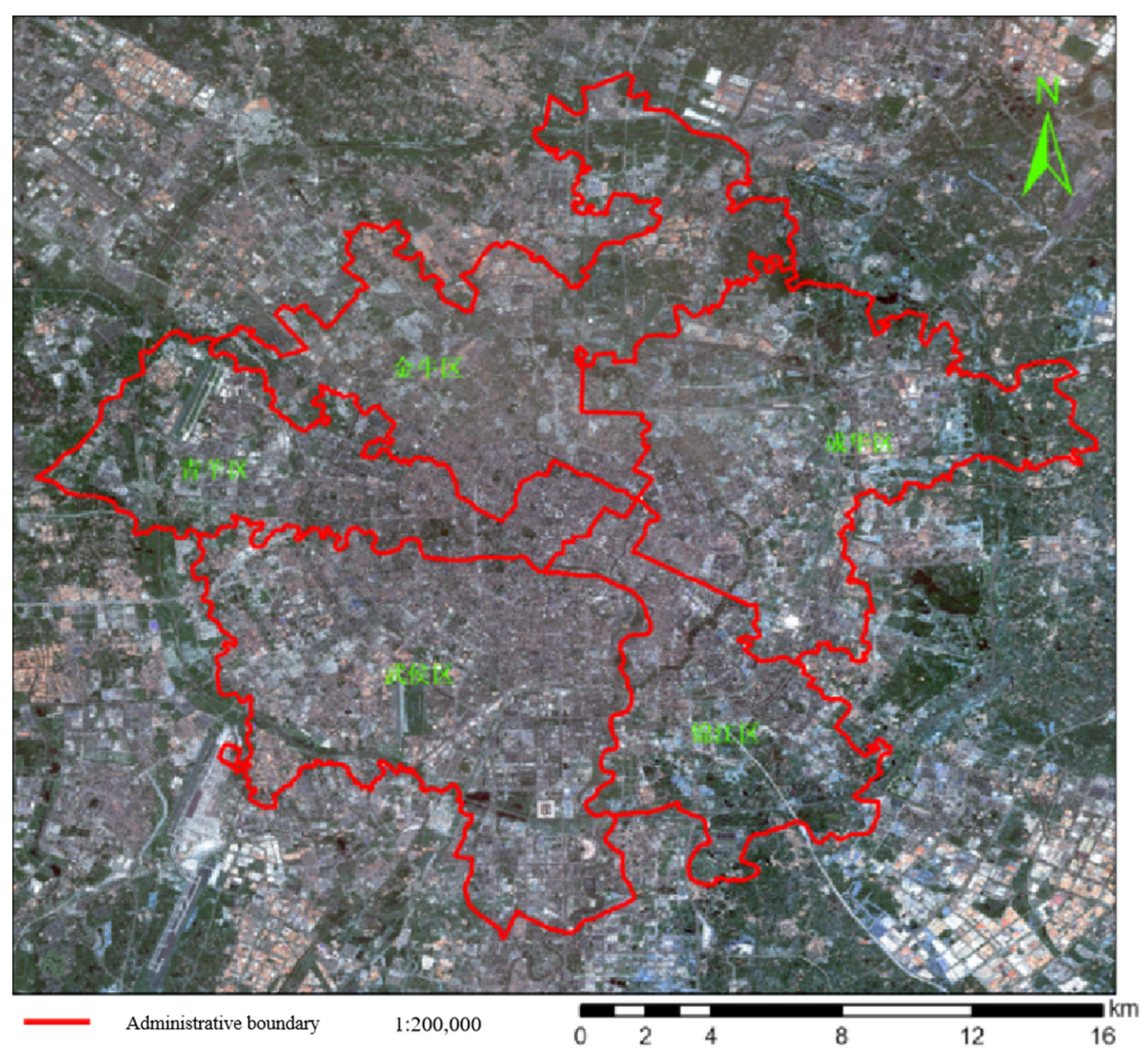
3.1. Study Area and Data Acquisition

The study area included selected core areas of the city of Chengdu, Sichuan Province, China: Qingyang District, Wuhou District, Jinjiang District, Jinniu District, and Chenghua District. The study area is located on a plain (103.9°E~104.2°E, 30.8°N~30.5°N) and is 464.7 km² large. Chengdu is the capital city of Sichuan Province and one of the earliest developed cities in southwestern China. With a high level of municipal infrastructure and public services, Chengdu is defined by the government as an important economic, science and technology, cultural and innovation, diplomatic, and transportation center in the western region of China [39]. Therefore, we chose Chengdu as the study area for analyzing and optimizing road congestion in large cities. Our research has significance in terms of demonstration and reference in traffic congestion management in large cities and medium-sized cities in China. The map of the study area is shown in Figure 1.

The data used in this study mainly included router vector data of Chengdu city and downtown from Amap.com, point-of-interest data from Amap.com and baidu.com, remote sensing images for the whole city, and data on the operating conditions of road traffic from documents from the administration department. Part of the data were used for quantitative analysis and extraction of road carrying capacity and vehicle conditions, while the rest were used to analyze the impact factors and spatiotemporal distribution of congestion and verify the effectiveness of the proposed method. The data used in this study are listed in

Table 1. Research data sources.

Data Category	Format	Area	Date	Coordinate System	Sample
Routers from Amap	Vector	Chengdu city	2015	GCJ-02
Routers from Amap	Vector	Main districts of Chengdu	2018	GCJ-02
POIs from Amap	Vector	Chengdu city	2015	GCJ-02
POIs from Baidu	Vector	Chengdu city	2018	B D-09
Actual operating conditions of road traffic	CSV	Chengdu city	2018	WGS-84
Remote sensing images	Raster	Chengdu city	2018–2019	WGS-84

.

3.2. Research Methodology

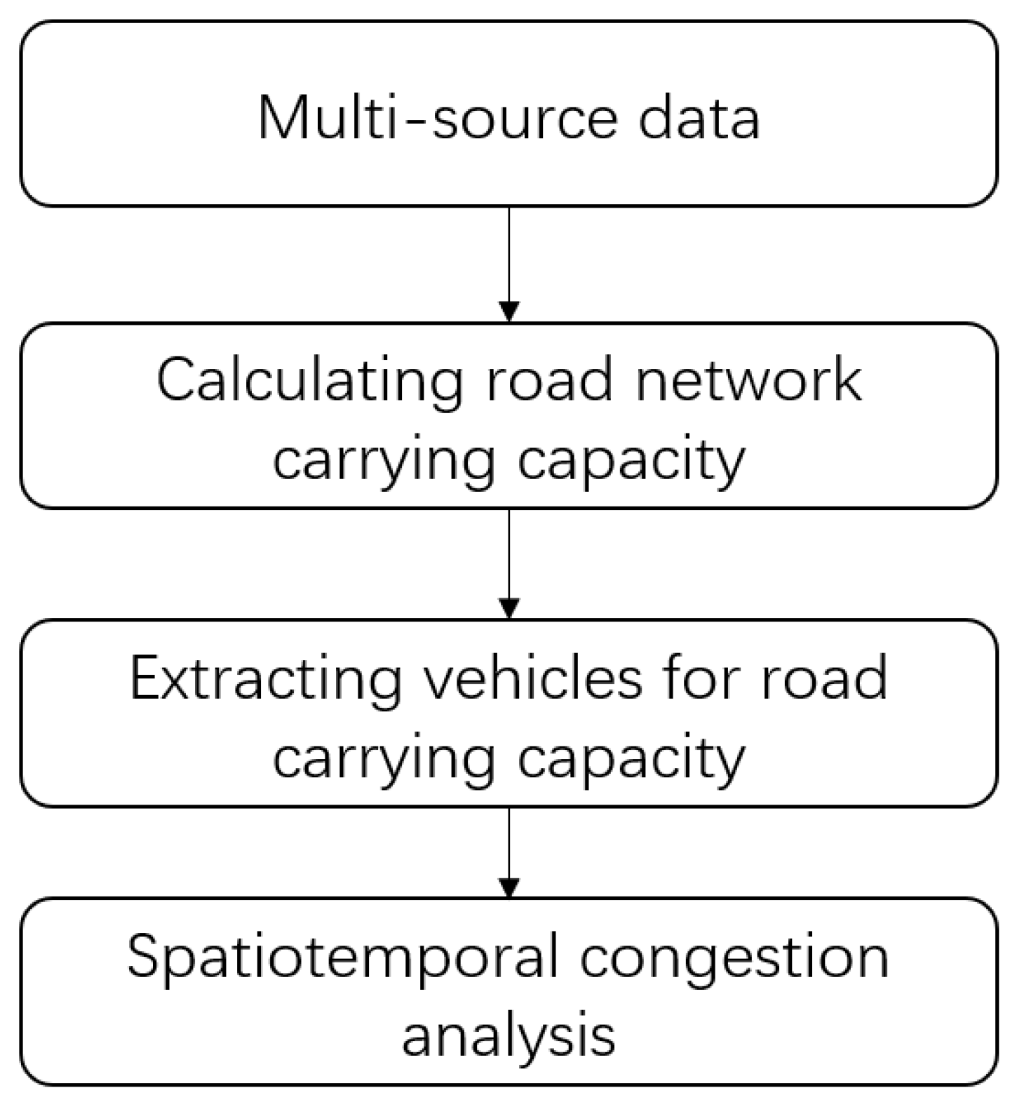
3.2.1. Overview of Proposed Method

In this study, we employed multi-resource data, including GIS vector data, high-resolution remote sensing data, and traffic operating condition data. We first applied the GIS data to calculate the road network carrying capacity for the research area; afterward, we extracted vehicle information for each road to calculate the carrying capacity and identify traffic congestion.The flowchart of the study is shown in Figure 2.

3.2.2. Calculation Model of Road Network Carrying Capacity

If we consider the geometric shape of a road to be a regular narrow belt or strip, the area of a road is approximately equal to the product of its length and width, and the calculation formula is

$$A=L·W$$

(1)

where A, L, and W are the area, length, and width of the road; the unit of length and width is kilometer.

We assumed that a vehicle is traveling at constant speed corresponding with the maximum speed designed for the road and that the number of lanes is ideally equal to the width of the road divided by the average width of the lane, with the result being forced to assume integral values.

Under ideal assumptions, the number of vehicles passing through a single lane is equal to the length of the road divided by the sum of the average length of the vehicles and the safe distance between them. If there are r types of roads in common, then the carrying capacity (C) of the entire road network is the sum of the carrying-capacity values of all roads, and the calculation formula is

$$C={{\displaystyle \sum }}_{j=1}^r{C}_j={{\displaystyle \sum }}_{j=1}^r{{\displaystyle \sum }}_{i=1}^n\frac{W_i}{\overline{w_i}}\frac{L_i}{l_i+s_i}$$

(2)

where C_j is the theoretical carrying capacity of the jth road; W_i and $\overline{w_i}$ are the width of the road and the width of lane, respectively; L_i is the length of the road; l_i and s_i are the average length of the vehicles and the safe distance between them, respectively, with i = 1, 2, …, n.

Thus, under certain road conditions, the width of the lane and the safe distance between two vehicles become the key factors restricting the carrying capacity of the road. l_i can be calculated from statistical vehicle data; s_i is directly related to the driving speed of a vehicle; W_i and L_i can be calculated from spatial data; and $\overline{w_i}$ can be determined in accordance with the state standards on road construction, with lane information extracted from high-resolution remote sensing images being employed for assessment. The maximum value of s_i was set according to national regulations, which means that when the vehicle speed exceeds 100 km/h, the safe distance is above 100 m; when the vehicle speed is below 100 km/h, the safe distance, in meters, is not lower than the spatial component of vehicle speed, in kilometers.

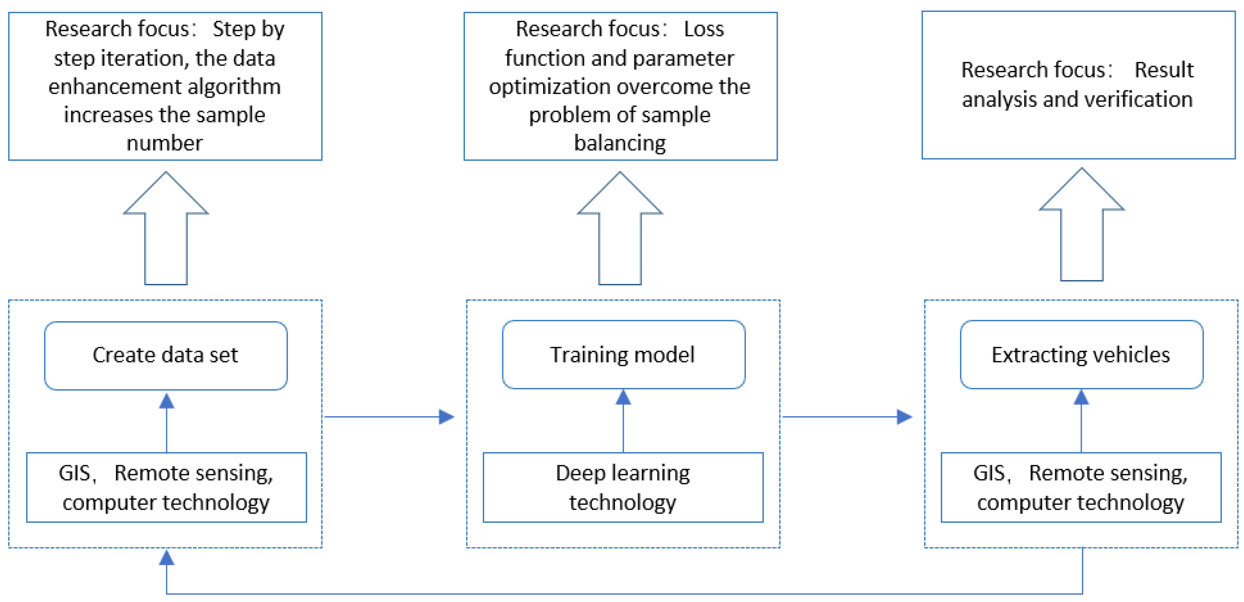
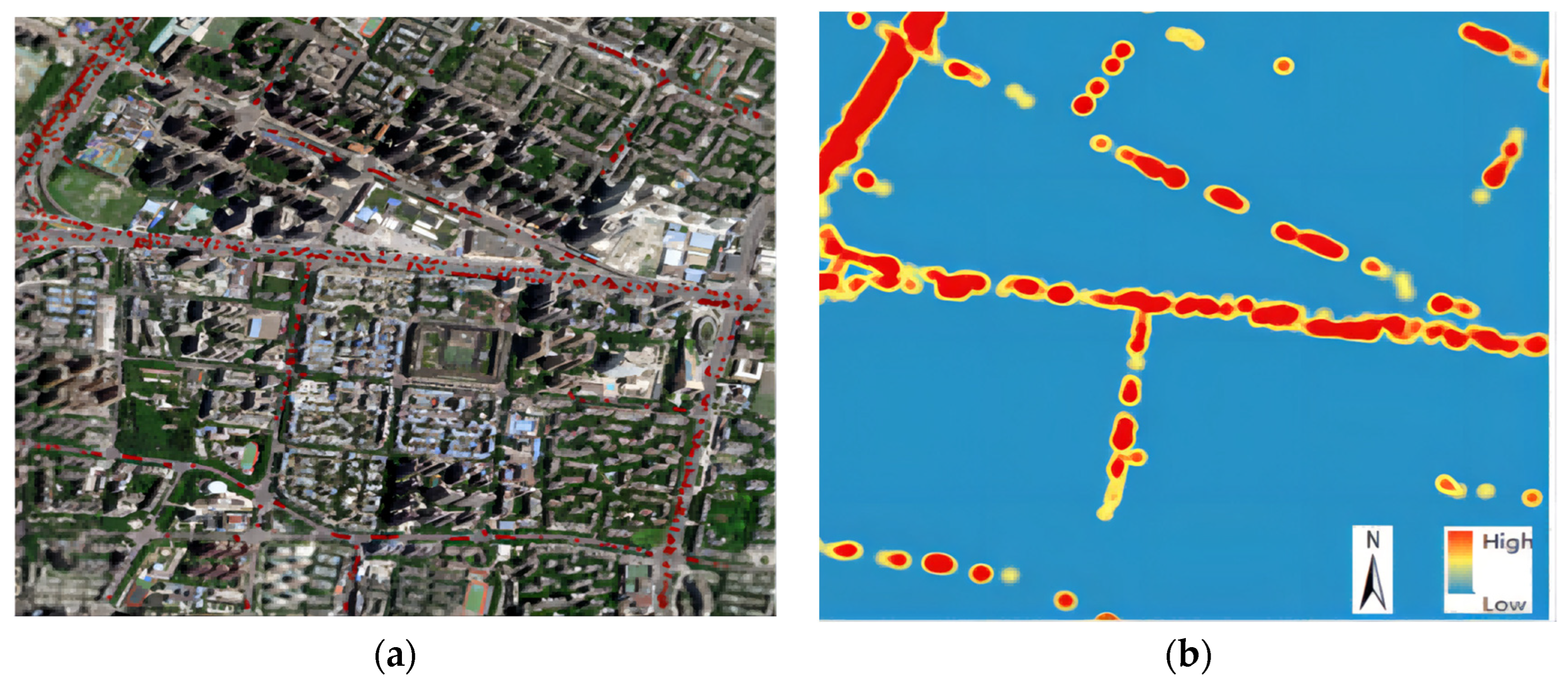
3.2.3. Calculation of Road Carrying Capacity Based on Number of Motor Vehicles

Deep learning is a method for learning data representation and modeling high-level abstractions in data. The basic network architecture proposed in this study is based on the that of two commonly used deep learning algorithms, U-Net and Retinanet. In order to optimize the data set construction process and the loss algorithm, we constructed a model for vehicle extraction from high-resolution remote sensing images. The overall technical framework is shown in Figure 3.

We employed the concept of probability density field [40] to measure the probability density distribution of each pixel in remote sensing images, analyze the contribution of samples to all pixels of the image in probability density, and control the weights of every category. The closer a pixel in the image is to the center point of the vehicle, the greater the probability of it belonging to the vehicle. Taking the spatial position of a pixel as a random variable, the probability density field was established by calculating the distance between the pixel and the center point of the vehicle, thus obtaining the probability of every pixel in the image belonging to the vehicle.

We used Equation 3 to calculate the density of the vehicles in the remote sensing images. The pixel density field kernel probability density function, F(x,y), was used to measure the probability density distribution of each remote sensing image belonging to a vehicle target. Pixels in remote sensing images were distributed discretely, so pixel coordinates (x,y) were discrete variables. According to the definition of probability density function, F(x,y) needs to satisfy two conditions, normalization and non-negativity, that is, the sum of the probability density function has to be equal to 1 throughout the entire domain, and the value of the probability density function must always be greater than or equal to 0. Therefore, F(x,y) needs to satisfy the following conditions:

$${{\displaystyle \sum }}_x{{\displaystyle \sum }}_{y}F\left(x,y\right)=1;F\left(x,y\right)\ge 0 \forall \left(x,y\right)$$

(3)

where F(x,y) is the pixel density field kernel probability density function, and x and y are the coordinates of any point P in the remote sensing image.

Then, the joint probability density distribution is

$$J\left(x,y\right)=\frac{1}{N_c}{{\displaystyle \sum }}_{j=1}^{N_c}F\left(x-x_j,y-y_j\right)$$

(4)

where N_c is the number of vehicle samples, and $x_j$ and $y_j$ are the coordinates of the center point of every vehicle sample, with j = 1, 2, …, $N_c$.

The closer pixel P is to the center point of the vehicle, the greater the probability of it belonging to the vehicle. In the same way, the farther its distance is, the smaller the probability of the point belonging to the vehicle. Therefore, the Gaussian function can be selected as the kernel function, and Formula (4) can be presented as

$$J\left(x,y\right)=\frac{1}{N_c}{{\displaystyle \sum }}_{j=1}^{N_c}\frac{1}{\sqrt{2\pi }}{e}^{\left(\frac{\left(x-x_j\right)+\left(y-y_j\right)}{2}\right)}$$

(5)

By using Formula (5), the probability density of each pixel in the image can be calculated as the weight of every category. Then, the loss function of vehicle extraction can be obtained with the following formula:

$$los{s}_{bfl}=\{\begin{array}{c}-J\left(x,y\right){\left(1-p_i\right)}^{\gamma }log{p}_i, i=1\\ -\left(1-J\left(x,y\right)\right)p_i^{\gamma }log\left(1-p_i\right),i=0\end{array}$$

(6)

where loss_bfl is the binary focal loss function for Gaussian function J, which controls the proportion of positive and negative samples; γ represents hyperparameters, which adjust the weights of difficult and easy samples; p_i is the predicted probability of class i samples; i is the label of the real sample, where 1 is positive and 0 is negative.

Figure 4 shows the probability density field results obtained using the proposed method.

3.2.4. A Spatiotemporal Analysis Method for Congestion Management through Calculation of Road Carrying Capacity

• A Road Network Carrying Capacity Balance Model Based on Geospatial Grids

A geospatial grid is a continuous unit grid with multi-resolution whose settings follow certain rules and whose uncertain spatial factors can be controlled within the corresponding scale range [41]. By constructing a road traffic geospatial grid, an integrated description of the spatial location and feature information of road traffic geographic entities can be realized.

In order to calculate the grid, it was first necessary to convert the spherical coordinate system into the Cartesian coordinate system. This is achieved with Formula (7), where X and Y are the projected Cartesian coordinate values, $L_{on}$ and $L_{at}$ are the longitude and latitude coordinates of the Earth’s surface, and G₁ and G₂ are the transformation functions:

$$\{\begin{array}{c}X=G_1\left(L_{on},L_{at}\right)\\ Y=G_2\left(L_{on},L_{at}\right)\end{array}$$

(7)

In the geospatial grid of an urban road network, each grid usually contains multiple roads; under certain conditions of road traffic and traffic control, if the number of vehicles entering the roads of a grid and that of vehicles exiting the roads of an adjacent one are consistent, then the total traffic flow in that urban area is considered constant. This is the basis of the conservation of regional traffic flow. Nine-palace-grid region analysis is a fast and effective method for determining the balance of regional road network carrying capacity. We propose a road network carrying capacity balance model based on geospatial grids. Taking into account the flow conservation concept by Lighthill [42], we defined the directions of the grid as either “in” or “out”, so that the number of vehicles departing from the center cell should be equal to the number of vehicles entering its adjacent eight cells within the nine-cell-grid model. If the road network carrying capacity of the central cell is greater than the total road network carrying capacity of its adjacent cells, then the former reaches a saturation state. Due to the inability of adjacent cells to carry the vehicles flowing out of the central cell, the regional road network becomes congested. In summary, the equilibrium of the regional road network configuration can be identified by analyzing the relationship between the carrying capacity of the central cell and the total road network carrying capacity of its adjacent 8 cells.

The encoding rule of the nine-cell-grid model is shown in Figure 5. The center cell is marked as S9, and the other grids are numbered clockwise as S1–S8. The road network carrying capacity of the entire area is equal to the sum of the road carrying capacity values of every cell. In the nine-cell-grid model, we defined Q as the ratio of the road network carrying capacity of the central cell to that of the other eight grid cells; thus, Q represents the rationality of the structure and configuration of the road network within this area. The calculation formula is

$$Q=\frac{C_{s9}}{C-C_{s9}}=\frac{{{\displaystyle \sum }}_{j=1}^r{C}_{s9,j}}{{{\displaystyle \sum }}_{m=1}^8{{\displaystyle \sum }}_{j=1}^r{C}_{sm,j}}$$

(8)

In the limit state, the minimum value of C_S9 is 0, which means there are no roads in the central cell. At this time, Q = 0, which means it is impossible to evaluate the regional road network configuration. Therefore, further analysis of the spatial configuration of the road network should be conducted in conjunction with the grids at different scales and the related road parameters. Conversely, Q = 1, which means that the carrying capacity of the central cell is equal to the total carrying capacity of the surrounding 8 cells; the road network configuration within this area reaches a critical state in theory. Based on the above assumption, without considering the departure of vehicles from the road network, the number of vehicles flowing out of S9 should be equal to the number of vehicles flowing into S9. When Q > 1, the number of vehicles flowing out of S9 is greater than that of the other 8 cells, resulting in a severely unbalanced road network configuration. When 0 < Q < 1, a smaller Q value indicates a better traffic configuration and a larger Q value indicates a worse traffic status in the nine-cell-grid area. Therefore, by analyzing the Q value, the equilibrium status of the regional road network spatial configuration can be identified; the Q value can be further used as a parameter for exploring the balance of carrying capacity.

For geospatial research at different scales, grids of different sizes and their combinations are usually designed. As shown in Figure 6, we constructed an equilibrium model with a combination of nine-cell grids at three levels, where the grid size at a higher level is one-third of that at a lower level. The construction process of the combination of nine-cell grids at three levels is shown in Figure 7. First, we divided study area A into 9 grid cells at the first level, where parameter Q of area A was obtained by calculating the carrying capacity ratio of 9 cells. Then, every grid cell at the first level was divided into 9 cells at the second level, and parameter Q of a grid at the first level was obtained by calculating the carrying capacity ratio of 9 cells at the second level. Therefore, we can obtain parameter Q at different levels in order to analyze the balance of road carrying capacity at different scales, especially for areas of interest, as shown in Figure 8, Figure 8a for small scale and Figure 8b for large scale.

2.

Analysis of spatiotemporal changes in urban road congestion and spatiotemporal detection of impact factors

Recently, real-time traffic data obtained using ArcGIS or QGIS have been increasingly used to study traffic congestion due to their advantages of comprehensive coverage, efficient updating, and flexible acquisition through multiple channels. By analyzing the overall traffic conditions of an urban road network, congested sections of roads can be identified. Furthermore, by integrating the real-time traffic conditions of surrounding roads and historical road condition data, the development trend of road conditions can be predicted and provided to users, such as drivers and pedestrians, who, in turn, also provide references for urban road network operation and management. In this study, we employed real-time traffic data from electronic navigation maps as the main data source to analyze the spatiotemporal changes in road congestion conditions and locations in large cities.

Spatial clustering and statistical algorithms were applied to analyze the spatiotemporal changes in congestion distribution during morning and evening peak hours and to determine the areas where congestion occurred frequently. Severely congested road sections were selected for spatial clustering analysis. Kernel density analysis, an important algorithm in spatial analysis, was used to calculate the spatial aggregation effect of spatial points or line elements. The entire research area was treated as a continuous density surface, and the density changes in elements within the search radius were automatically searched for and calculated in a certain window. The calculation formula is

$$f_h\left(x\right)=\frac{1}{n}{{\displaystyle \sum }}_{i=1}^n{w}_i{H}_h\left(x-x_i\right)$$

(9)

where $f_h\left(x\right)$ is the kernel density function, F denotes an independent distribution, $x_i$ is the sample point, n is the number of total sample points, $x-x_i$ is the distance between the calculated point and the sample point, $w_i$ is the power value, and h is the selected search radius.

Geographic detectors, a set of statistical methods based on the theory of geographic spatial differentiation, were used to detect the impact factors and driving mechanisms of the spatial patterns of geographical elements [43]. Compared with common statistical analysis methods, geographic detectors can demonstrate the similarity in spatial distribution between independent variables and dependent variables, which has significant impacts on the dependent variables. In this study, factor detection and interaction detection modules were used to explore the impact factors affecting vehicle driving speed and the interaction among different factors, respectively. The equation for the detection module is as follows:

$$q=1-\frac{1}{n{\sigma }^2}{{\displaystyle \sum }}_{i=1}^m{n}_i{\sigma }_i^2$$

(10)

where q is an impact factor affecting vehicle driving speed (value range of [0,1]), where the larger its value, the stronger its influence on vehicle driving speed; n is the number of grids; m is the number of types of impact factors; n_i is the number of grids with type i impact factors; σ is the variance in vehicle speed in all grids of the study area; σ_i is the variance in vehicle speed in grids of type i.

The ultimate goal of factor detection is to solve the bottleneck problem of congestion, and the impact factors selected for this goal should be quantifiable at a small spatial scale. From the perspective of road resource allocation, the impact factors were selected according to three objective aspects, which included the scale and structure of the road network, the connectivity and carrying capacity of the road network, and the scale and structure of public transport. Finally, the five impact factors selected included the density of the road network, node complexity, carrying capacity, and bus lines and the coverage rate of bus stops. In this study, we employed geospatial grids to spatially discretize factors using spatial information technology and detect the correlation between carrying capacity and other factors, providing a scientific basis for optimizing road resource allocation.

4. Case Study and Results Analysis

4.1. Analysis of Road Carrying Capacity Balance

The spatial statistics of the road network in the study area show that the average length of the road was 72 m and the maximum value of safe distance was 100 m. According to the traffic standard, we set the distance between the main roads to 800–1200 m and constructed three-level grids, with the first level of 3 × 3 km, the second level of 1 × 1 km, and the third level of 1/3 × 1/3 km. The structure and overlay of the nine-cell grids of different sizes are shown in Figure 5 and Figure 6, respectively. For the built-up area of Chengdu, the number of grid cells in the study area was calculated from the number of rows and columns. The resulting number of grid cells of the first level was 11 × 12 = 132; that of the second level was 33 × 36 = 1188; that of the third level was 99 × 108 = 10,692.

At the first level, the maximum carrying capacity of the grid was found to be 15,356 vehicles, and the minimum value, 5521 vehicles. At the second level, the maximum carrying capacity of the grid was calculated to be 2148 vehicles, and the minimum value 76 vehicles. At the first level, the average value of Q was calculated as 0.125, and the proportion of grid cells with a Q value greater than 0.125 was approximately 50%. The road network configuration within the area was assumed to be uniformly distributed, so the carrying capacity of the central cell was 1/9 of the total carrying capacity of the nine grid cells, and Q = 1/8 = 0.125. In this study, we took Q = 0.125 as the basis for determining whether the regional road network configuration was balanced. If Q > 1, the regional road network configuration was severely unbalanced and expected to experience congestion upon saturation of the carrying capacity of the central cell of the nine-cell-grid model. At the first and second levels, there were no grid cells with Q > 1. At the first level, there were 17 grid cells with Q > 0.125, and the maximum value of Q was 0.243. At the second level, there were 189 grid cells with Q > 0.125, and the maximum value of Q was 0.392. Figure 9 shows the distribution of Q values at the first level.

In this study, we obtained real-time urban traffic data from Gaode Map for verification and analysis. The top 10 congested roads within one week were selected, with a total of 8 roads being in the study area. At the first level, there were five road sections overlapping grid cells with Q > 0.125. Among these five roads, three road sections overlapped the area with the highest Q value, with the congestion rank orders of 1st, 5th, and 6th. At the second level, there were seven road sections overlapping grid cells with Q > 0.125, with an average Q value of 0.18. According to the grid analysis, the matching degree between the large-scale grid at the first level and the actual conditions was 62.5%, while that between the small-scale grid at the second level and the actual conditions was 87.5%.

The analysis of the correlation between the road network conditions and the carrying capacity ratio (Q) showed that at a 95% confidence level, there was a significantly negative correlation between morning and evening peak hours. The higher the Q value is, the greater the possibility of an unbalanced regional road network configuration, and the more likely a road is to be congested. A spatial matching analysis was conducted on the areas with Q > 0.125 and the areas frequently congested during morning and evening peak hours. At the first level, the proportion of road sections overlapping the marked grid cells was 68%, and at the second level, it was 73%. Therefore, the Q value can be used as an important reference indicator to purposefully optimize the allocation of road carrying capacity.

The main vehicles on urban roads are small cars. According to statistical data, the total number of vehicles in Chengdu was 4.35 million in 2018, of which 3.98 million were private cars, with nearly 90% being estimated to be small cars. Generally, the length of a small car is 4–5 m, with an average length of 4.5 m. The theoretical carrying capacity of the road network in the core areas of Chengdu was calculated to be 464,552 vehicles. Based on the natural breakpoint method, the carrying capacity per kilometer was divided into five categories. The spatial statistical results of every district are shown in Figure 10, where Figure 10a–e represent the visualization results of the road network carrying capacity grading for Wuhou District, Chenghua District, Jinniu District, Jinjiang District, and Qingyang District, respectively. The proportion distribution of road carrying capacity in each district and category showed certain similarities, with the section with the highest carrying capacity per unit length ranging from 20 to 50 vehicles, accounting for more than 30% of the total road length. The carrying capacity of most roads was 20–50 vehicles per kilometer, and these road sections accounted for over 30% of the total road length. Jinniu District had the highest carrying capacity, 35.82%, and Wuhou District had the lowest carrying capacity, 31.75%.

We firstly selected high-resolution remote sensing images of three time points to extract vehicle information for our experiment. Taking Wuhou District as an example, as shown in Figure 11, the numbers of vehicles extracted from the images of three time points were 2.2663, 4.0757, and 1.5886, respectively. The comparison of the theoretical carrying capacity and the actual vehicles on the road showed that the carrying capacity was greater than the number of actual vehicles on the road during non-peak hours; thus, the contradiction between road supply and vehicle demand was not obvious.

We matched the carrying capacity of the road network with the extracted road vehicle samples to the same 1 × 1 km spatial grid to calculate the matching degree between carrying capacity after grid transformation and actual transport vehicles, as shown in Figure 11. We then analyzed the spatiotemporal changes in the spatial distribution of supply and demand hotspots, from which we extracted heat maps. From the results, it can be seen that at the first time point, presenting relatively idle traffic (b), the conditions most closely matched the distribution of road carrying capacity (a). At the second time point, presenting peak traffic (c), the hotspots were concentrated within a radius of one kilometer around Tianfu Interchange. At the third time point, presenting relatively severe traffic (d), several traffic hotspots centered on Third Ring Road–Wuhou Avenue, Renmin South Road–Second Ring Road, Jiannan Avenue, and Tianfu Second Street formed.

Finally, we analyzed the spatiotemporal changes in road supply and vehicle demand in the hotspot areas, from which we obtained heat maps, as shown in Figure 12. Similar to the heat map results reported above, at the first time point, with relatively idle transportation, the traffic conditions were the most visually similar to the distribution of road carrying capacity. At the second time point, with mid-peak-hour transportation, the hotspot areas were concentrated within a radius of one kilometer centered on Tianfu Interchange. At the third time point, with relatively severe traffic, several hotspot areas appeared at the intersection of Third Ring Road and Wuhou Avenue, the intersection of Renmin South Road and Second Ring Road, Jiannan Avenue, and Tianfu Second Street.

4.2. Analysis of Road Congestion Status and Impact Factors

The road congestion status in Chengdu was analyzed using comprehensive geographic information technologies. Figure 13 shows the analysis results of the distribution of road congestion over different periods, i.e., a day and a week. On weekdays, the morning peak period was found to start at around 7:00 a.m. and reach its peak at around 8:00 a.m. The evening peak period was found to start at around 5:00 p.m. and continue until around 7:00 p.m. The morning peak period showed a trend of spreading from the surrounding areas to the central urban area, while the evening peak period showed the opposite trend. On weekends, traffic was different from that on weekdays, with the morning peak period appearing at around 9:00 a.m. and the evening peak period showing a longer duration.

During the week, congestion was the most severe on Monday and Friday, with the lowest average vehicle speed occurring on Monday, followed by Friday. Congestion during the evening peak period was more severe than that during the morning one because of the lower average vehicle speed and longer congestion mileage. During the week, the daily accumulated congestion mileage on weekdays was longer than that on weekends.

Figure 14 shows the extracted distribution maps of congested road sections during peak hours on weekdays. The extraction results of commonly congested areas in Chengdu as a whole are shown in Figure 15. There was a certain degree of similarity between morning and evening peak congestion areas, as well as significant differences. The southwestern section of Chengdu Ring Expressway outside Third Ring Road was a frequently congested area, with a clear trend of congestion during morning and evening peak hours. In the central urban area, the southern section of Second Ring Road presented a high incidence of morning and evening peak congestion. Overall, the congestion trend in the southeast of the core urban area was more pronounced during morning rush hours and that in the southwest was more severe during evening rush hours.

In order to analyze the traffic data of roads and vehicles at different times of the day, we selected vehicle speed as the dependent variable and five spatial indicators, including density of road network, node complexity, carrying capacity, density of bus lines, and coverage rate of bus stops, as the independent variables. The geographical exploration results are shown in

Table 2. Factor interaction results during morning peak hours.

Factor	Road Network Density	Bus Network Density	Node Density	Carrying Capacity	Bus Stop Coverage Rate
Road network	0.113632568
Bus network density	0.325978842	0.228960028
Node density	0.313461364	0.435280958	0.121162787
Carrying capacity	0.216198816	0.348898826	0.368858841	0.164306987
Bus stop coverage rate	0.433570493	0.473625342	0.446629476	0.405571841	0.315829605

. The explanatory power of each factor was the strongest at 8:00 a.m. and 6:00 p.m., while it was the weakest in the early morning and at 9:00 a.m.

The experimental results are consistent with the previous analysis of the congestion status. Among these five factors, the coverage rate of bus stops had the strongest explanatory power, with the value of 0.32 at 8:00 a.m. and the value of 0.29 at 6:00 p.m. during peak hours. The explanatory power of road network density was the weakest, with the value of 0.11 at 8:00 a.m. and the value of 0.09 at 6:00 p.m. during peak hours. Overall, the explanatory power of the five factors during peak traffic hours was ranked as follows: bus station coverage rate, bus network density, carrying capacity, node degree, and road network density. Lastly, the explanatory power of the node degree during idle traffic hours was greater than that of carrying capacity, as shown in Figure 16.

We further explored the interactive influence of the above factors. The type of interaction among various factors was classified into dual-factor enhancement mode and non-linear enhancement mode. We found no weakening nor independent relationship between any two factors, indicating that compared with the impact of a single factor, the dual interactions of different factor combinations had a stronger explanatory power for the spatial distribution of vehicle speed; in other words, the spatial distribution of vehicle speed was the result of the joint action of multiple factors. From the perspective of the role of single factors in dual-factor interactions, the influence of public transport factors on the interaction among factors was greater than that of other factors at 8:00 a.m. The interaction proportions between bus station coverage and road network density was above 0.4, and the interaction proportions between bus station coverage and node degree, the interaction proportions between bus station coverage and carrying capacity, the interaction proportions between bus network density and node degree/bus station coverage were all above 0.4; these results indicate that each of the above two factors of public transport had a strong impact on dual-factor interactions and greatly enhanced the influence of dual factors when combined with other factors. At 8:00 a.m., during morning peak hours, the interaction influence between bus station coverage and bus network density was 0.47, the interaction influence between bus station coverage and node degree was 0.45, the interaction influence between bus network density and node degree was 0.44, the interaction influence between bus station coverage and road network density was 0.43, and the interaction influence between bus station coverage and carrying capacity was 0.41.

There was significant spatial heterogeneity in the factors influencing vehicle speed. The impact of single factors on road traffic status varied significantly at different times and showed a certain regularity. As shown in Figure 17, the impact of road network density and node degree on vehicle speed was positive in idle traffic in the early morning. However, during peak traffic, the density of bus network and road carrying capacity increased, vehicle speed significantly decreased, and the impact of the node degree on vehicle speed first showed a negative trend and then a positive one.

According to the analysis of the equilibrium of road carrying capacity in Chengdu applied using the proposed method for congestion coordination, we advise that the node degree and public transport factors be combined to adjust the spatial distribution of bus stops in areas with a relatively high node degree. This adjustment is expected to optimize the resource utilization rate of congested road sections, achieve optimized resource allocation, improve travel efficiency, and thus increase road speed in congested areas.

5. Discussion

Methods for identifying and optimizing road congestion represent a challenging topic in interdisciplinary research. Traffic carrying capacity has dynamic, fuzzy, and uncertain characteristics, and its influencing factors have obvious spatiotemporal heterogeneity characteristics. In this study, we aimed at addressing existing needs of traffic management departments and travelers by combining GIS technology and the classic spatiotemporal consumption method [44] to construct an urban road carrying capacity analysis model based on geospatial data. Our method effectively solves the complexity and difficulty of obtaining historical model parameters and improves the accuracy and timeliness of calculations. Taking high-resolution remote sensing images as the research object, by detecting and identifying vehicle targets through this method, one can quantitatively analyze the actual number and spatial distribution of motor vehicles on the road on a large scale [45]. This traffic carrying capacity analysis method was designed from a spatiotemporal perspective, and a spatiotemporal balance analysis model of road network carrying capacity was constructed based on spatial geographic grids. Taking the regional balance of road network carrying capacity in Chengdu at different spatial scales as an example, we explored the spatiotemporal variation characteristics of the factors influencing carrying capacity and the spatial variation characteristics and rules of the dependent and independent variables [46], explaining the causal relationships among them. Compared with the actual congestion status, our analysis results achieve good accuracy. Thus, this method is effective in detecting traffic congestion in urban areas.

The advantage of the spatial nine-cell-grid-based equilibrium analysis model proposed in this study is that it can efficiently perform the dynamic calculation of the equilibrium degree at different spatial levels of the road network. Based on this, the established criteria for judging the equilibrium degree of regional carrying capacity can provide a basis for adjusting road supply capacity at the micro- and meso-levels. Based on a regional representation grid, the integrated description of the spatial positions and feature information of road traffic geographical entities can be achieved. Further, the use of spatial grids can provide a reference framework for the spatial location of transportation elements and represents a means of integrating various road traffic spatial information.

However, this method also has some shortcomings and limitations. For example, although it provides new solutions for analyzing road traffic supply optimization in the experiment, there may be inconsistencies in the experimental conclusions under conditions of complex road environments, management methods [47], etc. In this study, we only focused on the overall region, without considering the state of the road network, flow direction, attributes of urban areas, and other traffic facilities other than road traffic in the region in detail. As for the nine-cell-grid equilibrium model, its use only allows for the detection of problems from the perspective of road configuration itself. To avoid introducing too many parameter conditions, the following ideal assumptions were set: (1) vehicles in the nine-cell-grid area operated at a set speed; (2) the situation where vehicles leave the road network was not considered. In practical applications, when using the nine-cell-grid model to assess actual road vehicle conditions, it is necessary to further consider key factors such as road driving direction, entrances and exits, and large parking lots for vehicle allocation. In future work, traffic control data could be considered to further improve the matching of model and reality [48].

In addition, using high-resolution remote sensing data to extract vehicles has its own inherent limitations. For instance, the limitation of transit time on high-resolution remote sensing data makes it difficult to obtain morning and evening peak hour data. High-resolution data make it difficult for a single image to cover the entire research area, and extracting vehicles cannot strictly reflect the instantaneous distribution of vehicles. Due to the shadow of buildings and the obstruction of elevated bridges, there is a deviation in the estimated number of vehicles based on vehicle speed.

We compared the complexity requirements of previous models and those of our model in

Table 3. Comparison of the complexity requirements of previous models and our model.

Factors	Previous Models	Proposed Model
Road network key element extraction	Multi-steps using GIS tools and image processing tools	One-step extraction using deep learning method
Road network carrying capacity calculation	Difficulty in obtaining correction coefficients	Spatiotemporal analysis with grids to obtain results quickly
Balance analysis of regional road network carrying capacity	The inversion calculation of multiple types of data is complex and difficult	Nine-cell-grid balanced regression analysis

. The proposed method reduces the necessary steps for road network key element extraction for analysis. Further, our model uses grid computing for quickly performing road network carrying capacity calculations. Finally, the proposed method uses a nine-cell-grid regression analysis for easily accomplishing the balance analysis of regional road network carrying capacity.

6. Conclusions

From the perspective of spatial management, in this study, we propose a method for urban road carrying capacity calculation based on geospatial grids. The study area was divided into spatial grids of different sizes, nesting three levels of nine-cell grids. By calculating the carrying capacity ratio between the central cell and the surrounding cells in the nine-cell-grid model, the areas where the road network configuration may be unbalanced are identified. For our experiment, we took actual traffic operating condition data (dependent variables) and five spatial indicators (independent variables), including density of road network, node degree, carrying capacity, density of bus lines, and coverage rate of bus stops. The relationships among regional traffic conditions, impact factors, and spatial heterogeneity were analyzed. It was found that the proposed method effectively reduces the complexity requirements of parameters of previous theoretical models and the difficulty of obtaining such parameters; it also improves the accuracy and timeliness of the results, representing a new and quick processing technique for the planning of smart cities and smart transportation.

The method proposed in this study may represent a new solution for regional road traffic resource allocation. However, there may be inconsistencies between theoretical and experimental results because of the conditions of complex road environment, management methods, regional disequilibrium, etc.; therefore, more geographical and practical factors should be considered. Finally, in line with the significant existing research interest in traffic congestion, the following should be pursued in future work: the selection of impact factors needs to be further discussed; more types of urban and road traffic modes should be selected for further exploration; and the adaptability of this model needs further investigation.

References

1. Afrin, T.; Yodo, N. A Survey of Road Traffic Congestion Measures towards a Sustainable and Resilient Transportation System. Sustainability 2020, 12, 4660. [Google Scholar] [CrossRef]
2. Wei, X.; Shen, L.; Li, J.; Du, X. An alternative method for assessing urban transportation carrying capacity. Ecol. Indic. 2022, 142, 109299. [Google Scholar] [CrossRef]
3. Dubey, P.P.; Borkar, P. Review on techniques for traffic jam detection and congestion avoidance. In Proceedings of the 2015 2nd International Conference on Electronics and Communication Systems (ICECS), Coimbatore, India, 26–27 February 2015; pp. 434–440. [Google Scholar]
4. Song, J.; Zhao, C.; Zhong, S.; Nielsen, T.A.S.; Prishchepov, A.V. Mapping spatio-temporal patterns and detecting the factors of traffic congestion with multi-source data fusion and mining techniques. Comput. Environ. Urban Syst. 2019, 77, 101364. [Google Scholar] [CrossRef]
5. De-Ren, L. On Generalized and Specialized Spatial Information Grid. J. Remote Sens. 2005, 9, 513–520. [Google Scholar] [CrossRef]
6. Gao, P.; Liu, Z.; Tian, K.; Liu, G. Characterizing Traffic Conditions from the Perspective of Spatial-Temporal Heterogeneity. ISPRS Int. J. Geo-Inf. 2016, 5, 34. [Google Scholar] [CrossRef]
7. Shariff, M.A.; Faheem, M.I. A study on traffic carrying capacity of urban arterials under mixed traffic conditions. Int. J. Eng. Res. Ind. Appl. 2013, 6, 209–228. [Google Scholar]
8. Li, X.; Wang, L.; Fan, Y. Literature Review on Urban Road Traffic Carrying Capacity. J. Transp. Syst. Eng. Inf. Technol. 2022, 22, 15. [Google Scholar]
9. Jiang, D.; Zhao, W.; Wang, Y.; Wan, B. Analysis of urban road spatiotemporal situation by geographically weighted regression with spatial grid computing method. Geomat. Inf. Sci. Wuhan Univ. 2023, 48, 988–996. [Google Scholar] [CrossRef]
10. Gao, Y.; Qu, Z.; Song, X.; Yun, Z.; Zhu, F. Coordinated perimeter control of urban road network based on traffic carrying capacity model. Simul. Model. Pract. Theory 2023, 123, 102680. [Google Scholar] [CrossRef]
11. Iida, Y. Methodology for maximum capacity of road network. Transl. Jpn. Soc. Civ. Eng. 1972, 22, 147–150. [Google Scholar] [CrossRef]
12. Sumalee, A.; Kurauchi, F. Network capacity reliability analysis considering traffic regulation after a major disaster. Netw. Spat. Econ. 2006, 6, 205–219. [Google Scholar] [CrossRef]
13. Arasan, V.T.; Arkatkar, S. Derivation of capacity standards for intercity roads carrying heterogeneous traffic using computer simulation. Procedia-Soc. Behav. Sci. 2011, 16, 218–229. [Google Scholar] [CrossRef]
14. Chao, C.; Zhang, Y. Study on traffic carrying capacity of Tangshan city. In Proceedings of the International Conference on Computer Science and Service System (CSSS), Nanjing, China, 27–29 June 2011; pp. 2642–2646. [Google Scholar]
15. Fenton, R.E. A headway safety policy for automated highway operations. IEEE Trans. Veh. Technol. 1979, 28, 22–28. [Google Scholar] [CrossRef]
16. Yuan, Z.; Wang, T.; Zhang, J.; Li, S. Influences of dynamic safe headway on car-following behavior. Phys. A: Stat. Mech. Its Appl. 2022, 591, 126697. [Google Scholar] [CrossRef]
17. Kim, M.; Lee, J. A data transformation method for visualizing the statistical information based on the grid. Spat. Inf. Res. 2015, 23, 31–40. [Google Scholar]
18. Tollefsen, A.F.; Strand, H.; Buhaug, H. PRIO-GRID: A unified spatial data structure. J. Peace Res. 2012, 49, 363–374. [Google Scholar] [CrossRef]
19. Li, D.; Shao, Z.; Zhu, X. Spatial Information Multi-grid and Its Typical Application. Geomat. Inf. Sci. Wuhan Univ. 2004, 29, 945–950. [Google Scholar]
20. Shi, J.; Chen, L.; Qiao, F.; Yu, L.; Li, Q.; Fan, G. Simulation and analysis of the carrying capacity for road networks using a grid-based approach. J. Traffic Transp. Eng. 2020, 7, 498–506. [Google Scholar] [CrossRef]
21. Liu, Y.; Yan, X.; Wang, Y.; Yang, Z.; Wu, J. Grid mapping for spatial pattern analyses of recurrent urban traffic congestion based on taxi GPS sensing data. Sustainability 2017, 9, 533. [Google Scholar] [CrossRef]
22. Ye, S.; He, Z.; Jia, Y.; Luo, J. Analysis of spatial heterogeneity and influencing factors of urban traffic congestion based on gis. In Proceedings of the 2020 3rd International Conference on Geoinformatics and Data Analysis, Paris, France, 15–17 April 2020; pp. 48–52. [Google Scholar]
23. Lakshna, A.; Ramesh, K.; Prabha, B.; Sheema, D.; Vijayakumar, K. Machine learning Smart Traffic Prediction and Congestion Reduction. In Proceedings of the 2021 International Conference on Innovative Computing, Intelligent Communication and Smart Electrical Systems (ICSES), Chennai, India, 24–25 September 2021; pp. 1–4. [Google Scholar]
24. Yu, J.; Zeng, P.; Yu, Y.; Yu, H.; Huang, L.; Zhou, D. A Combined Convolutional Neural Network for Urban Land-Use Classification with GIS Data. Remote Sens. 2022, 14, 1128. [Google Scholar] [CrossRef]
25. Sharma, G.; Joshi, A.M.; Mohanty, S.P. sTrade: Blockchain based secure energy trading using vehicle-to-grid mutual authentication in smart transportation. Sustain. Energy Technol. Assess. 2023, 57, 103296. [Google Scholar] [CrossRef]
26. Li, Y.; Lin, H.; Jin, J. Decision-making for sustainable urban transportation: A statistical exploration of innovative mobility solutions and reduced emissions. Sustain. Cities Soc. 2024, 102, 105219. [Google Scholar] [CrossRef]
27. Harnischmacher, C.; Markefke, L.; Brendel, A.B.; Kolbe, L. Two-sided sustainability: Simulating battery degradation in vehicle to grid applications within autonomous electric port transportation. J. Clean. Prod. 2023, 384, 135598. [Google Scholar] [CrossRef]
28. Pan, X.; Dang, Y.; Wang, H.; Hong, D.; Li, Y.; Deng, H. Resilience model and recovery strategy of transportation network based on travel OD-grid analysis. Reliab. Eng. Syst. Saf. 2022, 223, 108483. [Google Scholar] [CrossRef]
29. Feng, T.; Liu, K.; Liang, C. An Improved Cellular Automata Traffic Flow Model Considering Driving Styles. Sustainability 2023, 15, 952. [Google Scholar] [CrossRef]
30. Wahle, J.; Neubert, L.; Esser, J.; Schreckenberg, M. A cellular automaton traffic flow model for online simulation of traffic. Parallel Comput. 2001, 27, 719–735. [Google Scholar] [CrossRef]
31. Zhang, S.; Shen, Y.; Zhao, Z. Design and implementation of a three-lane CA Traffic Flow model on ternary optical computer. Opt. Commun. 2020, 470, 125750. [Google Scholar] [CrossRef]
32. Jiang, Y.; Wang, S.; Yao, Z.; Zhao, B.; Wang, Y. A cellular automata model for mixed traffic flow considering the driving behavior of connected automated vehicle platoons. Phys. A Stat. Mech. Its Appl. 2021, 582, 126262. [Google Scholar] [CrossRef]
33. Thaysen, J.; Boisen, A.; Hansen, O.; Bouwstra, S. Atomic Force Microscopy Probe with Piezoresistive Read-out and a Highly Symmetrical Wheatstone Bridge Arrangement. Sens. Actuators A Phys. 2000, 83, 47–53. [Google Scholar] [CrossRef]
34. Toaza, B.; Esztergár-Kiss, D. A review of metaheuristic algorithms for solving TSP-based scheduling optimization problems. Appl. Soft. Comput. 2023, 148, 110908. [Google Scholar] [CrossRef]
35. Martínez-Salazar, I.A.; Molina, J.; Ángel-Bello, F.; Gómez, T.; Caballero, R. Solving a bi-objective Transportation Location Routing Problem by metaheuristic algorithms. Eur. J. Oper. Res. 2014, 234, 25–36. [Google Scholar] [CrossRef]
36. Khasawneh, M.A.; Awasthi, A. Intelligent Meta-Heuristic-Based Optimization of Traffic Light Timing Using Artificial Intelligence Techniques. Electronics 2023, 12, 4968. [Google Scholar] [CrossRef]
37. Waller, S.T.; Chand, S.; Zlojutro, A.; Nair, D.; Niu, C.; Wang, J.; Zhang, X.; Dixit, V.V. Rapidex: A Novel Tool to Estimate Origin–Destination Trips Using Pervasive Traffic Data. Sustainability 2021, 13, 11171. [Google Scholar] [CrossRef]
38. Olayode, I.O.; Tartibu, L.K.; Okwu, M.O.; Ukaegbu, U.F. Development of a Hybrid Artificial Neural Network-Particle Swarm Optimization Model for the Modelling of Traffic Flow of Vehicles at Signalized Road Intersections. Appl. Sci. 2021, 11, 8387. [Google Scholar] [CrossRef]
39. Rao, L.; Chen, F.; Zhou, H. Analysis of Traffic Accessibility in Tianfu New Area of Sichuan Province Based on Geographical Census. Geomat. Spat. Inf. Technol. 2019, 42, 72–74. [Google Scholar]
40. Li, J.; Cao, J.; Zhu, Y.; Cheng, B. Built-up area detection from high resolution remote sensing images using geometric features. J. Remote Sens. 2020, 24, 233–244. [Google Scholar] [CrossRef]
41. Peng, M. Division of Urban Spatial Information Multigrid Based on Hierarchical Spatial Reasoning. Geomat. Inf. Sci. Wuhan Univ. 2010, 35, 1112–1115. [Google Scholar]
42. Lighthill, M.J.; Whitham, G.B. On kinematic waves II. A theory of traffic flow on long crowded roads. Proc. R. Soc. London. Ser. A. Math. Phys. Sci. 1955, 229, 317–345. [Google Scholar] [CrossRef]
43. Wang, J.; Xu, C. Geodetector: Principle and prospective. Acta Geogr. Sin. 2017, 73, 219–231. [Google Scholar] [CrossRef]
44. Zhou, D.; Jiang, G.; Yu, J.; Liu, L.; Li, W. The Analysis of Task and Data Characteristic and the Collaborative Processing Method in Real-Time Visualization Pipeline of Urban 3DGIS. ISPRS Int. J. Geo-Inf. 2017, 6, 69. [Google Scholar] [CrossRef]
45. Tsitsokas, D.; Kouvelas, A.; Geroliminis, N. Modeling and optimization of dedicated bus lanes space allocation in large networks with dynamic congestion. Transp. Res. Part C: Emerg. Technol. 2021, 127, 103082. [Google Scholar] [CrossRef]
46. Przewozniczek, M.W.; Goścień, R.; Lechowicz, P.; Walkowiak, K. Metaheuristic algorithms with solution encoding mixing for effective optimization of SDM optical networks. Eng. Appl. Artif. Intell. 2020, 95, 103843. [Google Scholar] [CrossRef]
47. Almasi, M.H.; Oh, Y.; Sadollah, A.; Byon, Y.-J.; Kang, S. Urban transit network optimization under variable demand with single and multi-objective approaches using metaheuristics: The case of Daejeon, Korea. Int. J. Sustain. Transp. 2020, 15, 386–406. [Google Scholar] [CrossRef]
48. Liu, Q.; Li, X.; Liu, H.; Guo, Z. Multi-objective metaheuristics for discrete optimization problems: A review of the state-of-the-art. Appl. Soft Comput. 2020, 93, 106382. [Google Scholar] [CrossRef]
Figure 1. Map of the study area.
Ijgi 13 00059 g001
Figure 2. The flowchart of the study.
Ijgi 13 00059 g002
Figure 3. Technical framework of the proposed deep learning method for vehicle extraction.
Ijgi 13 00059 g003
Figure 4. Image classification based on probability density estimation. (a) Vehicle targets extracted from remote sensing images. (b) Probability density estimation of vehicle targets in remote sensing images.
Ijgi 13 00059 g004
Figure 5. Diagram of the nine-cell-grid model for regional road network configuration.
Ijgi 13 00059 g005
Figure 6. Three-level nine-cell-grid model of different sizes (red grid for the second level and the yellow grid for the third level).
Ijgi 13 00059 g006
Figure 7. Schematic diagram of the combination of nine-cell grids at three levels.
Ijgi 13 00059 g007
Figure 8. Analysis of the balance of road carrying capacity at different scales in the nine-cell-grid model. (a) for small scale of 1 × 1 km (nine numbers in blue circle note for nine-cell-grid), (b) for large scale of 3 × 3 km.
Ijgi 13 00059 g008
Figure 9. Distribution of Q values at the first level. (a) Q value distribution. (b) Grid cells with Q > 0.125.
Ijgi 13 00059 g009
Figure 10. Spatial distribution of road network carrying capacity at different levels in different districts of Chengdu. (a) Wuhou District; (b) Chenghua Distrcit; (c) Jinniu District; (d) Jinjiang Disctrict; (e) Qingyang Disctrict.
Ijgi 13 00059 g010
Figure 11. Comparison of supply and demand grid results for road motor vehicles in Wuhou District. (a) Carrying capacity. (b) First time point. (c) Second time point. (d) Third time point.
Ijgi 13 00059 g011
Figure 12. Supply and demand analysis of road carrying capacity in Wuhou District. (a) Carrying capacity. (b) First time point. (c) Second time point. (d) Third time point.
Ijgi 13 00059 g012
Figure 13. Spatial distribution of congested road sections during the day (red roads represent for congested).
Ijgi 13 00059 g013
Figure 14. Distribution of congested areas during morning and evening peak hours on weekdays. (a) Morning. (b) Evening.
Ijgi 13 00059 g014
Figure 15. Analysis of frequent congestion zones during morning and evening peak hours. (a) Morning. (b) Evening.
Ijgi 13 00059 g015
Figure 16. Changes in explanatory power of factors for major roads in Chengdu at different times.
Ijgi 13 00059 g016
Figure 17. Trends of impact factors relative to vehicle speed over time. (a) Impact of different times. (b) Impact of different factors on vehicle speed at the same times.
Ijgi 13 00059 g017