Article

Bayesian Structural Time Series and Geographically Weighted Logistic Regression Modelling Impacts of COVID-19 Lockdowns on the Spatiotemporal Patterns of London’s Crimes

CUSP London, Department of Informatics, King’s College London, London WC2B 4BG, UK
*
Author to whom correspondence should be addressed.
ISPRS Int. J. Geo-Inf. 2024, 13(1), 18; https://doi.org/10.3390/ijgi13010018
Submission received: 27 October 2023 / Revised: 28 December 2023 / Accepted: 28 December 2023 / Published: 4 January 2024

Abstract

:
Given the paramount impacts of COVID-19 on people’s lives in the capital of the UK, London, it was foreseeable that the city’s crime patterns would have undergone significant transformations, especially during lockdown periods. This study aims to testify the crime patterns’ changes in London, using data from March 2020 to March 2021 to explore the driving forces for such changes, and hence propose data-driven insights for policy makers and practitioners on London’s crime deduction and prevention potentiality in post-pandemic era. (1) Upon exploratory data analyses on the overall crime change patterns, an innovative BSTS model has been proposed by integrating restriction-level time series into the Bayesian structural time series (BSTS) model. This novel method allows the research to evaluate the varied effects of London’s three lockdown periods on local crimes among the regions of London. (2) Based on the predictive results from the BSTS modelling, three regression models were deployed to identify the driving forces for respective types of crime experiencing significant increases during lockdown periods. (3) The findings solidified research hypotheses on the distinct factors influencing London’s specific types of crime by period and by region. In light of the received evidence, insights on a modified policing allocation model and supporting the unemployed group was proposed in the aim of effectively mitigating the surges of crimes in London.

1. Introduction

To mitigate the impact of COVID-19 on the residents’ health and well-being, the UK government implemented a series of restrictions and policies in 2020 and 2021 to prevent the spread of the pandemic but with significantly influences on people’s behaviour patterns and psychological states [1,2,3,4,5,6,7,8]. Drawing upon criminological theories such as the routine activity approach and general strain theory, patterns of both acquisitive and expressive crimes may undergo noteworthy changes under such transitions, hence exhibiting varied patterns [9,10,11,12,13], attracting scholars to investigate the spatiotemporal changes in crime patterns between 2020 and 2021.
For instance, Abrams and Yang compared the United States’ crime data in 2019 and 2020 to examine the impact of lockdowns through time-series analysis [14,15] and found a rapid decline in all types of crime in 25 major US cities, except for the violent crime without any significant changes [14]. It is also testified that all acquisitive crimes in Chicago exhibited a pattern of initial decline during the lockdown but were then followed by a subsequent increase afterwards [15]. In addition to the analyses of historical recorded data, predictive studies also simulated counterfactual crime predictions without lockdown measures using models and compared them to real-world data [16,17,18]. For example, Kemp and colleagues utilised an ARIMA model to uncover the fact that COVID-19 restrictions in the UK led to a notable increase in cybercrime and fraud, although the impact varied among different types of fraud [16]. Furthermore, Paramasivan and colleagues enhanced the counterfactual prediction accuracy using an RNN model. Similarly to the findings of Yang et al., their results also demonstrated a significant decrease in acquisitive crime during the lockdown period, followed by a rebound after the restrictions were lifted [15,17].
In addition, some studies combined their spatiotemporal analysis approaches with mainstream crime research [15,16,17,18,19]. For example, Yang et al. employed SPPT and Moran’s I to examine changes in crime spatial patterns [15], Campedelli et al. innovatively used a logistic regression model to explore the marked reduction in crime in Chicago during the pandemic period and identified influencing factors, shedding some lights onto the methodological design for this research deploying regression models [19].
However, there were still some persistent crime issues that did not receive sufficient exploration. Firstly, the majority of studies focused on a pan-city analysis but missed the regional disparities at a finer scale [14,16,17,18]. Secondly, most research [15,16,17] has yet to attribute the effects of COVID-19 quantitatively, while they treated the pandemic as a singular observatory period for modelling, but overlooked the differences between various lockdown phases. In light of such lacunas, this paper has two main objectives.
The first objective is to quantify and analyse the impacts of COVID-19 on London’s crimes in specific areas. By integrating the methodologies of seasonal-trend decomposition using LOESS (STL), spatial panel pointtests (SPPTs), and local Moran’s I, a preliminary examination of the spatiotemporal changes of London’s crimes during the year 2020 was conducted. Furthermore, this paper employed the Bayesian structural time series (BSTS) model to assess the three lockdowns’ effects on crimes, respectively. The second objective was to analyse the underlying factors contributing to identified crime changes across various regions in London. Utilising the logistic regression (LR) and geographically weighted logistic regression (GWLR) model, this study analysed the factors contributing to the increase in crime during the lockdown periods in different Middle Super Output Areas (MSOAs).
The contribution of this study lies in its establishment of distinct BSTS models for evaluating crime changes during three different lockdown periods, which enables a comparative analysis measuring various influences on crime patterns in London during different stages of the pandemic. Secondly, the GWLR model, compared to traditional regression models, better accounts for the spatial autocorrelation among variables at localised scales, hence allowing researchers and practitioners to compare the varied impacts of selected influencing factors across different geographic regions (MSOAs).

2. Background

2.1. COVID-19 and Restrictions in England and London

The COVID-19 pandemic, as one of the most significant public health events in recent decades, has exerted profound global impacts. According to data provided by the UK government [1], in England, from the first identified case in January 2020 to August 2023, approximately 21 million confirmed cases and nearly 200,000 deaths were recorded—in London specifically, the capital and largest city in the UK, around 3 million confirmed cases were reported, resulting in approximately 26,000 deaths.
In response to the pandemic, the Greater London Authority (GLA) [2] took substantial measures to mitigate the threats posed by COVID-19. On 17 March 2020, the UK Prime Minister recommended working from home to the public, followed by the initiation of first lockdown on 24 March 2020 in England to mitigate the virus’s rapid spread. During this period, schools, pubs, shops, and restaurants were closed, and individuals were instructed to stay at home, with exceptions for essential venues; on 10 May 2020, the Prime Minister announced the conditional easing of the lockdown and work-from-home restrictions, signifying the end of first lockdown; hence, this period from March to May 2020 is considered as the first observation period to assess the impacts on crime changes.
With the emergence of the delta variant, England entered Tier 1 emergency status in October 2020. Subsequently, in November, the Prime Minister declared the start of a second lockdown lasting four weeks. Consequently, November and December 2020 were selected as the second observation period for this study. Later on, England entered into the third lockdown after the Christmas holiday until March 2021, when the Prime Minister issued a roadmap for gradually lifting restrictions. Thus, January–March 2021 is defined as the third observation period for this study.

2.2. Social and Economic Impacts of the Restrictions

Throughout the three observation periods, the closures of businesses and the implementation of social distancing due to COVID-19 restrictions incurred paramount impacts on the UK’s economy and employment market. According to statistics from the UK Office for National Statistics (ONS), the first lockdown led to a reduction of approximately 20% in both GDP and household expenditures, constituting the most significant decline in history [3], but both swiftly rebounded to normal levels once the lockdown was lifted. The effects of COVID-19 on employment rates were relatively mild in that UK unemployment rates only experienced a marginal increase (1.1%), reaching 5.2%, and subsequently continued to decline [4] from March to October 2020; such a phenomenon was considered to be attributed by Mayhew et al. to the job retention scheme introduced in May 2020, wherein employers could access 80% of furloughed employees’ wages [5]. Nonetheless, the resolution foundation’s research findings suggested that unemployment rates remained significantly high among low-income workers and young individuals [5,6].
On the other hand, social distancing also affected people’s mental well-being. Data from the UK Household Longitudinal Study (UKHLS) reveal that, compared to the same period in the preceding year, the number of adults experiencing psychological issues due to lockdown increased by nearly 10% [7]. Additionally, research by Chandola et al. indicated that the economic and psychological stresses brought about by lockdowns significantly elevated the incidences of common mental disorders, particularly among adults engaged in long-term remote work arrangements [8].

3. Related Work

In light of such, this study aimed to explore the pandemic-incurred impacts on London’s crime patterns by categorising the main crime types into acquisitive crimes (ACs) and expressive crimes (ECs). Acquisitive crimes refer to the premeditated illegal acquisition of others’ property, such as theft and robbery [9]; while expressive crimes represent those that generally lack a specific target and aim to vent personal negative emotions, including drug offences and violent crime [10]. Empirical studies had demonstrated significant variations in the impacts of COVID-19 restrictions on these two crime categories, and inspired the research hypotheses for this study to differentiate the impacts by their distinct motivations and natures.
On the basis of well-established classic theories in criminology, there are already theoretical foundations for explaining the notable shifts in crime patterns during the lockdown period in London. For example, Cohen and Felson’s routine activity theory captures the fact that shifts in crime trends are the results of changes in people’s daily routines and behavioural patterns [11,12]. Lockdowns brought forward significant alterations in people’s work and lifestyles, thus establishing prerequisites for changes in crime trends. The theory further highlights the direct interaction between offenders and victims as a crucial condition for predatory violations to occur [11]: for those affected by the social distancing policy, the absence of criminal opportunities is supposed to incur reductions in acquisitive crimes such as burglary, robbery, and theft [10]. Another theory proposed by Agnew, the general strain theory, posits that crime is related to the pressure and negative emotions (strain) that individuals experience in their lives, such as juvenile drug offences [13]. To reflect on the economic, psychological, and social pressures resulting from lockdowns [7,8], an increased risk of expressive crimes is predicted. Hence, this study is designed to explore the acquisitive and expressive crimes patterns in the case study city of London, as well as their connections and distinctions.
Inspired by such criminological theories, empirical studies have tried to examine the spatial and temporal impacts of COVID-19 restrictions on crime patterns. The current and ongoing temporal research could be broadly categorised into two approaches:
(1)
Some scholars compared the crimes’ time series during the lockdown with their historical series to observe the effects resulting from lockdown restrictions. For instance, Abrams employed difference-in-difference regressions to contrast crime time series between 2019 and 2020 in various US cities [14], and revealed decreases in most crime types in 2020, with notably drug offences exhibiting the most significant decrease, but violent crime being without distinct impacts from restrictions. Yang et al. utilised the Watson U² test to assess the similarity between Chicago’s crime time series in 2020 and that from 2016 to 2019. It also applied the Seasonal and Trend decomposition using the LOESS (STL) method to decompose a crime time series, allowing for a comparison of the composition of crime time series during the lockdown with historical data [15]. Findings showed substantial differences in the overall trend between crime time series and those of 2019, with the most acquisitive crimes exhibiting a trend of initial decline at the early stage of the lockdown, followed by an increase in crimes, and those significant outliers in crime time series were notably correlated with the issuance of restrictions [15].
(2)
Alternative temporal research approaches involve predicting counterfactual crime time series without the influence of lockdowns based on historical crime data, and quantifying the impact of lockdown on crime trends. In this regard, methods like ARIMA, BSTS, and RNN are mostly employed to forecast counterfactual crime time series. For instance, Kemp et al. conducted a counterfactual prediction using an autoregressive integrated moving average (ARIMA) model on the UK’s cybercrime and fraud crime data from the three years prior to the first lockdown [16]. The findings indicated that the actual counts of cyber and fraud crimes significantly exceeded the model-predicted values, suggesting a substantial crime increase due to lockdown. However, it is worth noting that different types of fraud crimes experienced varied impacts from the pandemic, such as ticket fraud, which relies on offline activities, and had significantly decreased [16]. This observation aligned with the hypothesis suggested by routine activity theory [11], but was found to be subject to data bias due to the lack of long-term regression analysis. Similarly, Paramasivan et al. employed a recurrent neural network (RNN) to predict and analyse the impact of India’s stay-at-home (SAH) policy on different crime types. Unlike ARIMA, the RNN model accounts for the effects of seasonality and holidays on crime time series [17]. As a return, the results indicated that the errors of the RNN model were significantly lower than those of the ARIMA and BSTS models. The RNN model’s performance on predicting acquisitive crimes were markedly higher than the actual values in an earlier lockdown period, signifying a significant reduction due to SAH; upon the lifting of the lockdown, actual counts of theft and robbery significantly exceeded the predicted values, suggesting an anomalous increase [17] afterwards. Therefore, this study would expect the analysis of changes in the two aforementioned crimes upon the lifting of lockdown restrictions. Moreover, Campedelli et al. employed a Bayesian structural time series (BSTS) model for the counterfactual prediction of Los Angeles crime data. The study incorporated temperature and holiday time series as covariates to mitigate the influence of seasonality and noise on model fitting. The findings revealed that the most acquisitive crimes, except for burglary, significantly decreased during lockdowns. Conversely, expressive crimes, except for intimate partner assault, did not change significantly [15,18].
Building on the content outlined above, standard time series analysis could be employed to investigate general shifts in crime trends, such as at the aggregated geographical level [17]. Contemporary empirical studies tend to further integrate spatial analysis into time series analysis in the aim of better capturing the regional impacts of lockdowns on different regions within a target city. For example, Yang et al. employed the spatial point pattern test and Moran’s I to assess the spatial changes in Chicago’s crimes, and the results obtained indicated that alterations in crime spatial patterns were primarily localised with the emergence of new crime clusters during the lockdown [15]. Campedelli et al.’s study in Chicago managed to evaluate the impact of social distancing on crimes, and innovatively combined the BSTS model with Firth’s logistic regression [19], and successfully established respective BSTS models for unique census tracts in Chicago to evaluate whether significant increases in crime occurred during the lockdown. It also employed Firth’s logistic regression to analyse the transformed binary data from BSTS, and was therefore able to investigate the potential factors contributing to significant reductions in crime during the lockdown. However, the study’s limitation lies in adopting a global regression model, which overlooks the crime’s spatial autocorrelation [19]. This study draws inspiration from their work and aims to analyse the factors influencing London’s crime changes by combining the BSTS model with a regression model. Another work performed by Wang et al. combined the BSTS model with a geographically and temporally weighted regression model (GTWR) to analyse the impact of the lockdown on Beijing’s subway passenger flow. It brought further insights into this study for effectively analysing the impacts of lockdown on varied locations at different times, considering the spatial correlation of the subway passenger flow [20], which was deemed suitable for analysing the spatiotemporal crime patterns’ changes and identifying the potential influencing factors.

4. Approach

4.1. Workflow

As illustrated in Figure 1, there are three milestone research steps in the workflow of research design. This study is initiated from identifying the spatiotemporal variations in London’s crime patterns during the pandemic period. Historical crime data and the results from the seasonal and trend decomposition using the LOESS (STL) method were combined to examine the changes in crime trends, seasonality, and residuals both prior to and after the lockdown. Meanwhile, the spatial point pattern test (SPPT) model was deployed to assess the alterations in the spatial distribution of London’s crimes between 2019 and 2020 in line with the utilisation of local Moran’s I to investigate shifts in crime hotspots. The second step is designed to quantify the impact of COVID-19 restrictions on crime counts using the Bayesian structural time series (BSTS) model, to assess the influence of restrictions on both the overall crime counts in London and in London MSOAs among the three lockdown periods. Based on the outcomes derived from the BSTS model, the third step employs logistic regression (LR) and geographically weighted logistic regression (GWLR) models to analyse the factors contributing to significant increases in crime counts across various MSOAs. Additionally, the project delved into criminogenic or crime-mediating demographic and socio-economic factors to analyse their impacts on the different types of crimes in London during the three lockdown periods.

4.2. Data

4.2.1. Study Area

London, the capital city, is a study area with approximately 607 square miles and a population of 8.8 million [21]. According to 2021 UK Census data, London is divided into 983 Middle Super Output Areas (MSOAs) (Figure 2), and this study adheres to the geographical boundary data published by the Greater London Authority in 2011 [22,23]. It was recorded that each MSOA encompasses a resident population of 5000–15,000 individuals, distributed among 2000–6000 households [23]. However, due to the absence of the City of London in the crime data provided by the Metropolitan Police, 982 MSOAs (excluding the City of London) are included in this study.

4.2.2. Crime Data

The crime data utilised in this study were provided by the Metropolitan Police [24], spanning from March 2011 to July on a monthly basis at the MSOA scale, to encapsulate the monthly occurrences of eleven distinct crime types among 982 London MSOAs. In pursuit of the comprehensive representation, this paper selected three acquisitive crimes (burglary, robbery, and theft) and two expressive crimes (drug offences and violence against the person) for in-depth investigation. Table 1 illustrates the definitions assigned by the Metropolitan Police to selected crime types [25]. The crime data used in this article refer to the number of crimes.
This study uses point-based crime location data to construct the spatial point pattern test (SPPT) model, enabling an analysis of alterations in the crime point patterns across London. To facilitate this endeavour, we included London’s crime data from 2011 to 2021, provided by data.police.uk (accessed on 5 May 2023) [26], including the information on the temporal features (year–month), precise geographical coordinates, and the categorisation of crimes for all occurrences within London. In addition, London’s stop and search data from data.police.uk were also included in the model, to evaluate the efficacy of stop and search, including similar information on the timing (year–month) and geographic locations of stop and search instances [26].

4.2.3. Holiday and Temperature Data

Given the notable impact of variations from holidays and temperature (seasonality) on specific types of crime [13,18], this study incorporated these two factors as covariates in the BSTS model. Temperature data were sourced from Weather Spark, encompassing London’s monthly average maximum and minimum temperatures from 2011 to 2021 (as depicted in Figure 3a). Holiday data were derived from the holiday library in Python to include the count of bank holidays every month in the UK from 2011 to 2021, forming a time series of holiday occurrences (illustrated in Figure 3b).

4.2.4. COVID-19 Restriction Time Series

It is assumed that the impacts may vary by restrictions and lockdown policies among the target periods, so this study incorporates the COVID-19 restrictions time series provided by the Greater London Authority to capture lockdown restrictions from March 2020 to January 2022. For example, seven distinct restriction measures are documented as: school closures, pub shut-downs, shop closures, restaurant shut-downs, staying at home, household mixing indoors banned, and working from home [2]. Given that the data on restriction levels are organised on a weekly basis, the restriction level for each week was calculated by counting the quantity of varied restriction measures in place during the target week. For example, if a week experienced three types of restrictions, namely school closure, pub shutdown, and shop closure, then its restriction level is valued as 3. And, being align with the crime data, the monthly average restriction level is also a covariate in the designed BSTS model.

4.2.5. Demographic and Socio-Economic Data

This study managed to assess the demographic and socio-economic features on the alteration of crime patterns during London’s lockdown periods. The data were primarily derived from the 2021 Census data released by the ONS [27] at the MSOA level. Key variables include age, gender, population density, unemployment rates, and the proportion of households in poverty. The population density is the number of permanent residents per square kilometre. Given the contextual backdrop, the pandemic brought about a relatively inconspicuous decline in the overall unemployment rate in the UK, while individuals already grappling with unemployment and economic hardships faced heightened pressures [5,6]. As a result, this study assesses the employment status of individuals within MSOAs by examining the proportion of those who were employed and those who were not employed in the past 12 months. Furthermore, as evidenced by current research, a pronounced link exists between the population mobility and crime that has been identified, particularly with respect to acquisitive crimes during lockdown periods [17,28]. Thus, we utilised the reduction in mobility across the various boroughs of London during the pandemic, from Google Mobility data, as a predictive variable in the regression model [29].

4.3. Methods

4.3.1. Seasonal and Trend Decomposition Using LOESS (STL)

Findings from Yang et al.’s work suggest that COVID-19 restrictions exert an influence on urban crime patterns’ trend, seasonality, and residuals [15]. Thus, contrasting trends, seasonality, and residuals prior to and after lockdowns can offer enhanced insights into the impact of restrictions on the temporal patterns of crime. The seasonal and trend decomposition using the LOESS (STL) method was introduced by Cleveland and Devlin in 1990 [30], as an intuitive approach for time series decomposition. During the decomposition process, it disassembles the time series ( Y v ) into trend ( T v ), seasonality ( S v ), and residual ( R v ) components using third-order locally estimated scatterplot smoothing (LOESS) [15], as illustrated in Equation (1), where the trend represents the overall direction of data variation, seasonality captures repetitive patterns, and residuals encapsulate anomalies that cannot be accounted for by the two other components.
Y v = T v + S v + R v
To improve the precision of the model performance, this study employs London’s monthly crime data from April 2016 to March 2023 for model building and testing; and a seasonal period of 12 months is designated for the model in light of the crime data’s monthly recorded nature. The implementation of this model is facilitated through the utilisation of the STL function from the Statsmodels library in Python.

4.3.2. Spatial Point Pattern Test (SPPT)

The spatial point pattern test, introduced by Andresen in 2016, is usually employed to compare disparities in spatial point data patterns between the different time frames for the same geographical region [31]. The model’s philosophical foundation is to compare the proportion of point data (e.g., crime points) within all geographical regions (MSOAs) of a target city, between the base year and test years. For this specific study, 2019 is set to be the base year, with 2020 being the test year; in 2020, the model further employed a Monte Carlo simulation (200 iterations, each with an 85% sampling rate) to consider a 95% confidence interval for the proportion of crimes in each MSOA. When the proportion of crime occurrences in a given MSOA during the base year, 2019, falls into the confidence interval of the same MSOA during the test year in 2020, the model will then denote these two MSOAs as comparable [31].
S = i = 1 n s i n
In addition to aforementioned localised measurements among London MSOAs, this model also enables the assessment of disparities for the whole of London between 2019 and 2020 by using the index of similarity (S) depicted in Equation (2), where s i represents a binary variable denoting whether the crime distribution in an MSOA is similar between 2019 and 2020, and n signifies the total number of MSOAs in London. Thus, the index of similarity portrays the proportion of MSOAs that exhibit similarity between the two years. As S approaches closer to 1, it signifies a higher resemblance in crime patterns between the years 2019 and 2020 in London [31]. The parameters in the model were set to their default values according to a program developed by Nick Malleson [32].

4.3.3. Moran’s I

The Global Moran’s I index is utilised as a metric to quantify the overall spatial autocorrelation [33] and is expressed as in Equation (3).
I = N i j w i j ( x i x ¯ ) ( x j x ¯ ) i j w i j i ( x i x ¯ ) 2
In this context, the variable under investigation is represented by x, which is the crime count in MSOAs. x ¯ denotes the mean of x, signifying the average crime count across all MSOAs. N represents the total count of points against target MSOAs. The w i j represents the values in the spatial weight matrix (with i and j denoting its row and column position in the weight matrix, respectively), indicating the spatial relationships between distinct MSOAs, and Queen Contiguity is adopted to define adjacency relationships among MSOAs. The values of global Moran’s I range from −1 to 1, with values approaching absolute 1 indicating stronger spatial autocorrelation, and the sign indicating positive or negative correlations. A further examination of its pseudo p-value with a value of less than 0.05 will imply significant spatial autocorrelation [34]. Furthermore, local Moran’s I had been used to assess the spatial autocorrelation strength among different MSOAs, thereby to identify the presence of crime clustering phenomena. The calculation formula for local Moran’s I is presented in Equation (4), with the variables holding the same significance as in Equation (3).
I i = N ( x i x ¯ ) j w i j ( x j x ¯ ) i ( x i x ¯ ) 2
In receiving local Moran’s I for crimes across all London MSOAs, the LISA clustering method had been applied to further categorise the outcomes into four groups: high–high clusters, high–low outliers, low–high outliers, and low–low clusters; with particular interest been paid to those MSOAs in the high–high category. Additionally, an increase in the crime count in one MSOA suggests a likely increase in others as well.

4.3.4. Bayesian Structural Time Series Model (BSTS)

One of the objectives for this study is to ascertain whether the lockdown intervention has resulted in a notable increase in crimes in London. In light of the fact that the Bayesian structural time series (BSTS) model, serving as an inferential framework for assessing causal relationships, is frequently employed to determine the significant effects of interventions during specified timeframes [35], the model could be ideal to make predictions on counterfactual crime time series in the absence of lockdown measures to compare the predicted and actual sequences of lockdown, and to discern the presence of a significant increase in crime in a predictive scenario. As formulated as Equation (5),
y t = μ t + S t + β T x t + ε t
where y t represents the variable under prediction, which, in this context, pertains to the counterfactual crime time series. The BSTS regression equation consists of trend ( μ t ), seasonality ( S t ) and residual terms ( ε t ) [36] with the regression component ( β ) being of particular interest. x t signifies a time series associated with the crime time series. This incorporation of additional covariates enhances the prediction accuracy of the crime time series.
To further improve the crime time series model, some studies incorporated covariates such as holiday and temperature data for counterfactual prediction. This strategy allows the BSTS model to better account for the disturbances arising from factors like holidays and climatic variations compared to methods like ARIMA and RNN. In line with this approach, our study utilises monthly average temperatures (both highest and lowest) and the count of holiday days from March 2011 to March 2021 in London as covariates for the BSTS model. However, existing research has a notable limitation in generating a single counterfactual prediction curve for the entire lockdown period; for example, in Figure 4, by Troy Smith et al., the blue-dashed line represents the counterfactual murder crime prediction generated by the BSTS model [37]. In this sense, the prediction may be biased to sudden changes incurred by the first lockdown, whilst it is well acknowledged that London had indeed experienced three lockdowns, with each posed by distinct policies; it further made the universal modelling risky in overlooking potential inter-lockdown disparities.
In light of the above, this study incorporated the restriction level as a covariate by computing the average weekly COVID-19 restriction level for each month from March 2020 to March 2021. This enabled us to compare the impacts from three lockdowns on crimes in London. For instance, drying the month before the initiation of the second lockdown in November 2020, the average restriction level in London was 3.25, so the average restriction level for November 2020 and all subsequent months will be set at 3.25. This approach draws inspiration from interrupted time series analysis, albeit substituting the dummy variable representing intervention with the restriction level [38]. Within this framework, separate models were fitted for each of the three lockdowns utilising crime historical data from distinct periods. The pre-intervention and post-intervention periods for each lockdown were outlined in Table 2. To enhance curve fitting, the model was trained using monthly crime data dated back to March 2011. Furthermore, to achieve a more comprehensive analysis of the varying impacts of the three lockdowns on different crime types, three BSTS predictions were conducted for the time series of diverse crimes within each MSOA. The modelling process was executed using R’s CasualImpact library, with the seasonal parameter set at 12, while retaining default values for other parameters.
At last, two metrics were utilised to present the results of the Bayesian structural time series (BSTS) model, which are (1) the relative cumulative impact (RCE) [19], as shown in Equation (6), where y i represents the observed monthly crime counts during the lockdown period, and y ^ i denotes the predicted value. The cumulative difference between the observed and predicted values was computed during the post-intervention period of the lockdown, divided by the sum of the predicted values. The absolute value of RCE thus indicates the magnitude of the impact of the lockdown on crime counts, while its sign indicates the direction of the impact (increase/decrease).
RCE = i y i i y ^ i i y ^ i
Additionally, the p-value of the BSTS model was selected as a crucial assessment criterion, with a value of less than 0.05 indicating the significant impact from the lockdown on crime.
S I = 0 R C E 0 p 0.05 1 R C E > 0 p < 0.05

4.3.5. Logistic Regression Model

Logistic regression is a variation of linear regression. Still, it employs a logistic function (the sigmoid function) to transform the continuous linear output into probability values between 0 and 1. Consequently, logistic regression is particularly handy for binary classification problems. The logistic regression equation is illustrated in Equation (9).
P ( Y = 1 | X ) = 1 1 + e ( β 0 + β 1 X 1 + β 2 X 2 + + β p X p )
In this context, we can break down the components as follows: P ( Y = 1 | X ) represents the probability of observing class 1, where X denotes the input feature vector. Additionally, β 0 serves as the interception term, while β 1 , β 2 , , β p are the coefficients that characterise the influence of each variables.
The logistic regression model produces a probability. Samples with probabilities above 0.5 are classified as class 1 ( Y = 1 ), and those at or below 0.5 are classified as class 0 ( Y = 0 ). This versatility makes the logistic regression valuable for diverse classification tasks.

4.3.6. Geographically Weighted Logistic Regression

On top of the RCE and p-value through the significantly increased ( S I ) variable (Equation (7)), th-geographically weighted logistic regression (GWLR) model was established to identify those MSOAs that witnessed significant crimes increases by selecting those with an RCE greater than 0 and a p-value below the significance level of 0.05; conversely, an increase is considered insignificant when the RCE is not greater than 0 and the p-value is above 0.05.
The GWLR model is an extended variant of the geographically weighted regression (GWR) by constructing local regression models for each geographical region based on the observations of the target region itself and its neighbours [39], where the so-called neighbours bear higher weights if they are closer to the target. The regression equation for each region is illustrated in Equation (9).
ln ( p i 1 p i ) = β i 0 + k β i k ( u i , v i ) x i k + ε i
where β i k ( u i , v i ) represents for the coefficient of the kth predictor variable for the ith geographical region, and x i k denotes the observed value of the kth predictor variable for the same target region. Additionally, β i 0 stands for the intercept of the region’s regression equation, while ε i signifies the residual term [39]. Unlike the GWR model, GWLR deals with a binary response variable (categories 0 and 1), and thus the predicted outcome is the probability falling into named category 1, denoted by p i in Equation (9). Drawing inspiration from logistic regression principles, GWLR employs the sigmoid function to map the linear regression values onto the interval [0, 1] for predicting p i .
In this study, we employed the S I index generated from the BSTS model as the response variable for GWLR, and which allows the prediction of significant probability on crime growth in each MSOA during the three lockdown periods; the regression coefficients of the equation were designed to capture the relationship between different predictor variables and the significant increase in crimes, where the odds ratio (OR) was adopted as a measure for this relationship (Equation (10)).
O R i k = e β i k
where β i k retains its role as the coefficient of the kth predictor variable for the ith geographical region. O R i k represents for a positive value greater than 0, but indicates a negative correlation between the variable k and the risk of crime growth, when it is less than 1, with a stronger correlation the more it approaches 0. On the contrary, when it exceeds 1, a positive correlation between variable k and the risk of crime growth will be interpreted, with a higher value implying a stronger correlation. By adopting the OR of each MSOA, it is now possible to assess which potential factors affect the risk of increased crime during the lockdown periods [40].

5. Results

5.1. Temporal and Spatial Shifts in Crime Patterns

5.1.1. Temporal Variations

Figure 5 depicts the time series of crime incidents in London from 2019 to 2023. The grey-dashed lines P1, P2, and P3 represent the starts of the three respective lockdowns, while P4 represents the time point at which all restrictions were lifted. It is obvious that the implementation of social distancing policies during the first lockdown significantly reduced crime incidents, which plunged to their lowest historical levels in April 2020. In May 2020, following the conditional lifting of the first lockdown, crime incidents rapidly bounced back and peaked in July before another gradually slowing down. From November 2020 to January 2021, during lockdown 2 and lockdown 3, crime incidents sharply dropped again but rebounded since February 2021.
An in-depth look into the representative types of crimes in London is presented in Figure 6, where the time series of different types of crime incidents, including burglary, theft, robbery, and violence against persons, exhibit similar trends. Each of them experienced a decline following the start of a lockdown and rebounded after restrictions were lifted. Notably, the number of thefts showed a particularly significant change, which was consistent with the findings from Yang et al. in Chicago. The conclusion could be drawn that, at this stage, acquisitive crimes experienced a sharp decline during the initial stages of the lockdown but rebounded upon the lifting of restrictions [15]. On the other hand, drug offences in London displayed a distinctive pattern, with a significant increase only observed after lockdown 1, but followed by stable fluctuations thereafter. This finding was in contrast to Abrams et al.’s observations in finding drug crimes among 16 American big cities that experienced significant decreases during the lockdown period [14].
To further analyse the impact of the lockdown on the time series of crime incidents, STL decomposition was deployed to separate the crime incident data into trends, seasonality, and residuals. As illustrated in Figure 7b,d,f, the trend component indicates that acquisitive crimes (burglary, theft, and robbery) experienced a significant reduction during the lockdown due to social distancing policies and the closure of commercial areas, leading to decreased opportunities for crime. However, according to Figure 7c,e, expressive crimes (drug offences and violence against persons) exhibited an increasing trend which may be due to the psychological and economic stress incurred by isolation measures. It is also noteworthy that burglary and drug offences after the lifting of restrictions. Drug offences and burglary experienced a sharp decline to their lowest levels, while violent crime stabilised and ceased to increase since December 2021. On the contrary, the number of theft and robbery incidents significantly increased after April 2021, which suggested that the police force may prioritise crimes with higher social harm and costs in the earlier stage following the lockdown, leading to less attention being paid to crimes with relatively lower impacts.
The seasonal component shows that each type of crime exhibited a distinct seasonal pattern which did not appear to be significantly affected by COVID-19 restrictions. Theft and violence against the persons had typical peaks during the spring and summer months, and reached at their lowest levels in the winter. Drug offences and robbery crimes peaked during the summer and remain relatively stable throughout the other seasons. On the other hand, burglary and other crime types have more significant variations, often with two peaks in the autumn and winter but declined to lower levels in the spring and summer. The seasonal component confirms that seasonal and temperature variations will notably influence the occurrence of crime incidents, hence suggesting the inclusion of temperature as a covariate in the BSTS model in the aim of generating a predictive curve of crime incidents without the intervention of restrictions, and further to capture the seasonal patterns, especially the influence of temperature on crime trends.
The final residual component reveals the distribution of outliers in the discussed crime time series. Burglary, robbery, and theft showed significant negative outliers following lockdown, which further confirmed that restrictions led to an exceptional decrease in acquisitive crimes. As people became used to the lockdown routine activities, outliers decreased in volume and frequency; however, such a pattern was not evident for expressive crimes. Although negative residuals were also observed for expressive crimes during lockdowns, there was a notable positive outlier upon the lifting of the lockdowns (April 2020 and August 2021). Similarly, drug offences also showed an abnormal increase during the first lockdown, which may owe to the accumulated stress and tension out from prolonged social distancing, and the increase in expressive crimes; as well as the positive extreme values that occurred after restrictions were lifted.
Temporally, the COVID-19 restriction policies have different impacts on various types of crime in London. Burglary, robbery, and theft, the named acquisitive crimes, were easily influenced by the decrease in social activities, with their crime volumes significantly changing alongside the level of restrictions. On the other hand, expressive crimes experienced abnormal increases during lockdowns, but with exceptional violent crime being affected by reduced social activities, and hence decreases during lockdown and abnormal growths post-lockdown due to the potential release of negative emotions and pressure.

5.1.2. Spatial Variations

The results of the SPPT test (Table 3) indicated a global similarity index at 0.14 between 2019 and 2020, which was notably lower than the outcomes for the two other groups (2017 vs. 2018 and 2018 vs. 2019), suggesting a more pronounced shift in the spatial distribution of crimes between 2019 and 2020. Among all crime categories, the most noteworthy spatial disparity lay in theft, with a global ‘s’ value merely measured at 0.16. In comparison with the previous years’ similarity index, it became evident that theft displayed the most substantial spatiotemporal alterations among all crime types. Moreover, violent crimes also experienced a slight decrease in the similarity index compared to its preceding period. Consequently, both theft and violence underwent more conspicuous spatial distribution changes in terms of how they were affected by the pandemic.
Figure 8 describes the spatial changes for various types of crimes across the MSOAs of London by comparing 2020 and 2019, where the colour blue indicates a decrease in the crime proportion for the target region in 2020 against 2019; red highlights an increase in crime; and grey signifies a non-significant similarity index.
Table 4 presented the Global Moran’s I values for the volumes of crime in London in 2019 and 2020. Global Moran’s I provides insight into the overall spatial autocorrelation, with values closer to 1 indicating a more clustered spatial distribution of crimes. Given that the p-values for all results are less than 0.05, there is a significant spatial autocorrelation in the distribution of all crime types across London. Notably, the Global Moran’s I for the total crime count in 2020 is 0.41, signifying the persistence of crime hotspots even during the pandemic. Additionally, both the total crime incidents and the Moran’s I values for the three acquisitive crimes exhibited a slight decrease, while the global Moran’s I for expressive crimes showed a marginal increase compared to 2019.
Figure 9 illustrates the Local Moran’s I values for different crime types across the MSOAs of London. Red areas exhibit “high–high” clusters, or so-called “hot spots”, indicating that both the target areas themselves and their surrounding neighbourhoods have high crime rates. This pattern suggests regions with frequent criminal activity, possibly due to specific socio-economic or environmental factors. Conversely, the blue areas show “low–low” clusters, or so-called “cold spots”, meaning that both these regions and their adjacent areas have lower crime rates. This may indicate better community management, a higher sense of safety, or other crime deterrent factors in place. Examining the total crime count, similarly to 2019, crime hotspots in London during 2020 predominantly cluster in central boroughs such as Westminster, Camden, Islington, Hackney, and Tower Hamlets. However, Hackney and Tower Hamlets experienced an increased number of crime hotspots compared to 2019. Moreover, a sizable high–high cluster emerged at the boundary of Ealing and Brent in 2020. This region also serves as a hotspot for drug offences and violence against persons. Concurrently, a new high–high cluster for the total crime count, drug offences, and violent crime arises at the boundary between Haringey and Enfield. Finally, attention is drawn to a shared high–high cluster of burglary, drug offences, robbery, and violent crime on the northwest side of Croydon in 2020. This cluster demonstrates a notably expanded trend compared to 2019, particularly for the two expressive crimes.

5.2. The Impact of COVID-19 on the Spatiotemporal Patterns of Crime

5.2.1. Temporal Impact

Expanding on the preceding spatial and temporal analyses, we establish a noticeable shift in the spatiotemporal crime patterns in London during the year 2020. The upcoming results from the Bayesian structural time series (BSTS) model aim to quantify and examine the extent to which this alteration is connected to the implementation of lockdown measures.
Figure 10 illustrates the outcomes of BSTS modelling for London’s total crime time series from March to May 2020, corresponding to the initial lockdown period. In Figure 10a (original), the grey line represents the actual crime time series, while the orange line portrays the counterfactual prediction curve in the hypothetical scenario in which there are no COVID-19 restrictions.
It is noticeable that, due to the inclusion of monthly average temperature and holiday numbers, the prediction curve for the pre-intervention period aligns remarkably well with the actual time series, indicating a favourable model fit. However, starting from March 2020, the actual crime count begins to deviate notably below the projected count.
The red-dashed lines in the figure demarcate the start and end of the first lockdown. Figure 10b illustrates the absolute differences between the actual crime data and counterfactual predictions. Figure 10c displays the relative impact of the lockdown on the crime count, indicating the percentage of the absolute impact against the predicted crime count. By combining these insights from Figure 10b,c, it is evident that the restrictions imposed during lockdown 1 led to a sharp decline in absolute impact, signifying a substantial reduction in the crime count compared to the baseline. Specifically, in April, the restrictions contributed to a decrease in crime count of approximately 25,000 cases (approximately 35% of the predicted value without restrictions). By the end of May, lockdown 1 had cumulatively resulted in a reduction of approximately 57,000 instances of crime in London.
Figure 11 illustrates the results of the BSTS model for lockdown 2. By integrating the restriction level time series as a covariate in the BSTS model, the orange curve in Figure 11a represents the predicted crime curve assuming a constant level of restrictions as they were in October. Since lockdown 2 spanned only one month and featured specific restrictions (such as working from home and a curfew) in October, its impact is notably reduced compared to the effects of lockdown 1. In November 2020, the crime count was reduced by approximately 3100 cases in contrast to the scenario without lockdown, constituting around 5% of the total (as demonstrated in Figure 11b,c).
Moving to Figure 12, the modelling outcomes for lockdown 3 are presented. As shown in Figure 12a, if the restriction level remains unaltered after the end of lockdown 2, crime counts would cease their decline in January 2021 and instead display stable fluctuations. Lockdown 3 led to a reduction of around 13% in the predicted crime counts for January (Figure 12b) and a decrease of about 9.4% in February. While the decline in crime counts resulting from lockdown 3 are more noticeable compared to that for lockdown 2, it remains substantially less impactful than the effects observed during the initial lockdown period (lockdown 1).

5.2.2. Spatial Impact

To examine the impact of COVID-19 restrictions on crime counts across various regions of London, separate BSTS models were developed for different types of crimes in each MSOA.
Figure 13 presents the outcomes of the BSTS models for the total crime counts in each MSOA during the three lockdowns. The red shading indicates a significant increase in crime counts during lockdown 1 (RCE > 0 and p-value < 0.05), while blue shading represents a significant decrease (RCE < 0 and p-value < 0.05), and grey shading signifies non-significance (p-value > 0.05). Deeper colours correspond to larger absolute values of RCE, indicating greater increments or decrements. Appendix A Figure A1 and Figure A2 depict the top 10 boroughs with the lowest and highest average RCE values for different crime types across the three lockdowns, illustrating the boroughs with the most notable decreases and increases in crime counts attributed to lockdown impacts.
Consistent with the findings from our temporal analysis, lockdowns 1 and 3 had the most pronounced effects on crime counts across London, resulting in a significant reduction in crime counts in approximately 34% and 28% of MSOAs, respectively, (Appendix A Table A1). In contrast, lockdown 2 led to nearly equal proportions of MSOAs with significant increases and decreases (10% and 14%, respectively). In terms of spatial distribution, the MSOAs experiencing the most substantial reductions in crime counts during the three lockdowns were concentrated in Westminster, at the heart of London, and its neighbouring boroughs (Appendix A Figure A1). Notably, crime counts around Heathrow Airport also displayed significant reductions. Conversely, the MSOAs significantly affected by increases in crime were evenly distributed in areas closer to the city’s periphery (such as the northern part of Hillingdon in lockdown 1, and Enfield and Croydon in lockdown 2). It is worth highlighting that these areas encompassed many newly emerged hotspots of expressive crimes, particularly in the case of Croydon.
Figure 14 depicts how the spatial distribution of MSOAs was significantly impacted by the three distinct types of acquisitive crime. Similarly to the overall crime counts, a greater number of MSOAs experienced significant reductions in acquisitive crimes during the first and third lockdowns. Among the acquisitive crimes, MSOAs witnessing significant changes, particularly reductions, were more numerous for burglary and theft compared to robbery. As seen in Appendix A Figure A1, MSOAs where burglary significantly decreased were primarily located in the city’s periphery, including boroughs like Bexley, Hillingdon, and Kingston upon Thames, while central areas had relatively fewer such instances. In contrast, MSOAs with a significant decrease in theft were concentrated in the city centre, with some presence in the western and southwestern boroughs such as Kingston upon Thames and Bromley.
However, during the second lockdown, there was a noticeable increase in the number of MSOAs exhibiting statistically significant increases in both burglary and theft. Notably, a substantial area of significant increase in burglary was observed on the eastern side of Richmond upon Thames, with multiple clusters apparent in Lewisham. In the case of theft, a significant increase was mainly situated in the northeast and western regions of London, particularly in Hillingdon. Furthermore, during the third lockdown, the intersection between Barnet and Enfield saw a significant number of MSOAs with a noteworthy increase in theft.
In contrast, the number of regions with a statistically significant change in robbery was limited. Similarly to the other two acquisitive crime categories, robberies continued to significantly decrease in MSOAs located in the city centre. Notably, in each of the three lockdowns, certain MSOAs within the eastern part of Bromley, Enfield, and Barnet witnessed extreme and statistically significant increases, with magnitudes more than doubling.
Figure 15 portrays how the spatial distribution of MSOAs was significantly impacted by two distinct categories of expressive crimes due to the lockdown measures. Unlike acquisitive crimes, the majority of significantly impacted MSOAs experienced notable increases in expressive crimes, particularly in the case of drug offences.
The proportion of MSOAs exhibiting a significant increase in drug offences during the first lockdown (approximately 42%) surpassed that observed during the second and third lockdowns. Notably, in the first lockdown, the deep red-shaded MSOAs were evenly distributed throughout the city centre and densely populated along the periphery areas such as Havering, Bromley, Hillingdon, and Sutton. Meanwhile, the city centre exhibited a sparser distribution. As lockdown 2 commenced, the MSOAs with significant increases in drug offences became less prevalent around the southwestern and western peripheries of the city centre, while areas like Hillingdon, Enfield, and Havering still exhibited a greater prevalence. During lockdown 3, some MSOAs close to the city centre, such as Haringey, Islington, and Lewisham even experienced significant decreases in drug offences. However, the areas with significant increases remained more prevalent in the western and eastern outer peripheries of the city centre.
In comparison to drug offences, the number of MSOAs with a significant increase in violence against persons was relatively fewer and with milder magnitudes. In the first lockdown, deep red-shaded MSOAs were primarily distributed in remote regions to the northwest, north, and south of London (e.g., Hillingdon, Enfield, and Sutton). Additionally, MSOAs with significant decreases constituted 7% during lockdown 1, although the extent of reduction was modest (see Appendix A Table A2). During lockdown 2, MSOAs with significant increases shifted notably away from the western areas, while more areas exhibited deep red-shaded regions in the north and south. During lockdown 3, the distribution of violent crime resembled that of lockdown 1, albeit with slight reductions in the deep red-shaded regions to the north and southwest. Notably, certain MSOAs within the city centre, particularly in Westminster, exhibited a consistent pattern of a significant decrease across all three lockdowns.

5.3. Contributors to the Increase in Crime during Lockdowns

5.3.1. Spatial Autocorrelation and Multicollinearity

To address the potential issue of multicollinearity among variables, the variance inflation factors (VIFs) were calculated for all independent variables. For any given model, except for the variable “Aged 60 years and over”, which exhibited a slightly higher VIF (of approximately 6), all other variables had VIF values well below 5 (see Appendix A Table A3). This suggests a lack of severe collinearity among the independent variables.
To initially examine the spatial autocorrelation and contributors to the significant crime increases during the three lockdown periods in London, this study first established logistic regression models for different crime types based on the BSTS results. It assessed the spatial autocorrelation of their residuals. The Moran’s I of model residuals is presented in Table 5. Notably, for the two expressive crime categories, the model residuals exhibited statistically significant spatial autocorrelation during all three lockdown periods (p-value < 0.05). This signifies that the global logistic regression models are inadequate in explaining the spatial heterogeneity underlying these two crime types [41]. Consequently, we intend to analyse the potential factors leading to the significant increase in these crimes through the GWLR model. Conversely, since the residuals of the three acquisitive crime categories did not show significant spatial autocorrelation (p-value > 0.05), we will directly analyse them using the outcomes of the global models.

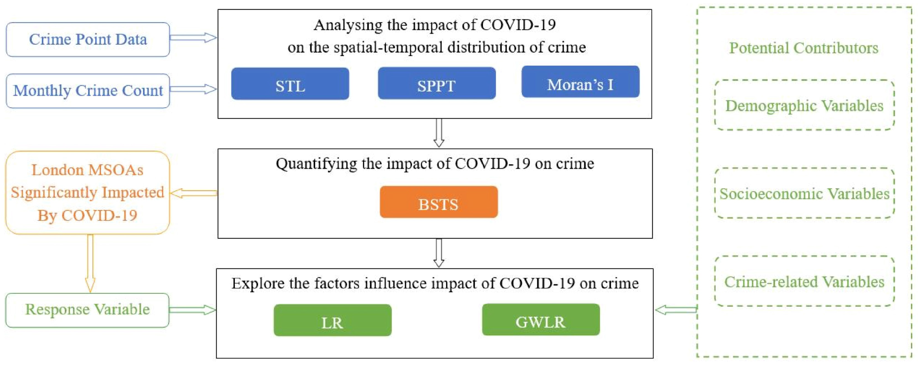
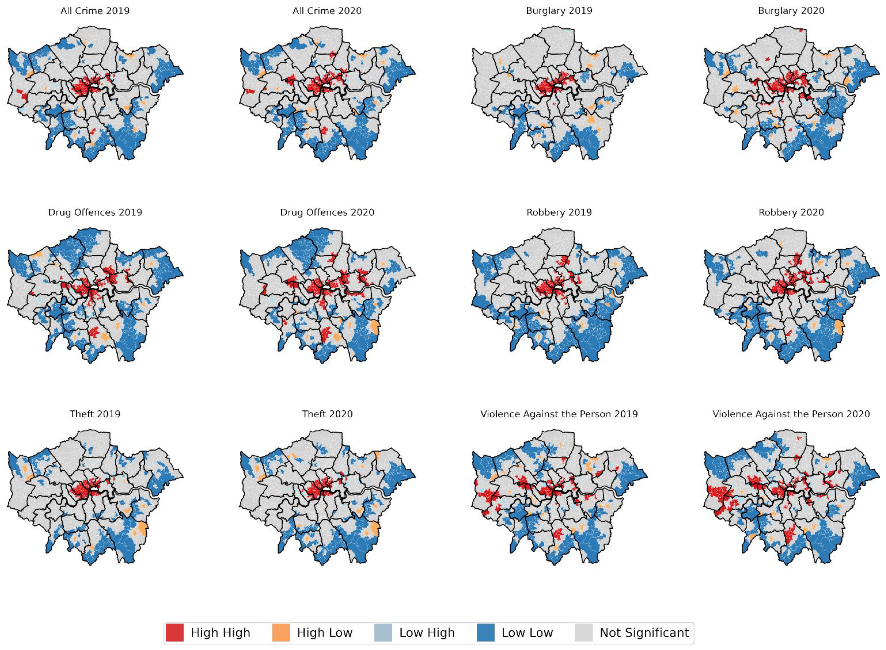
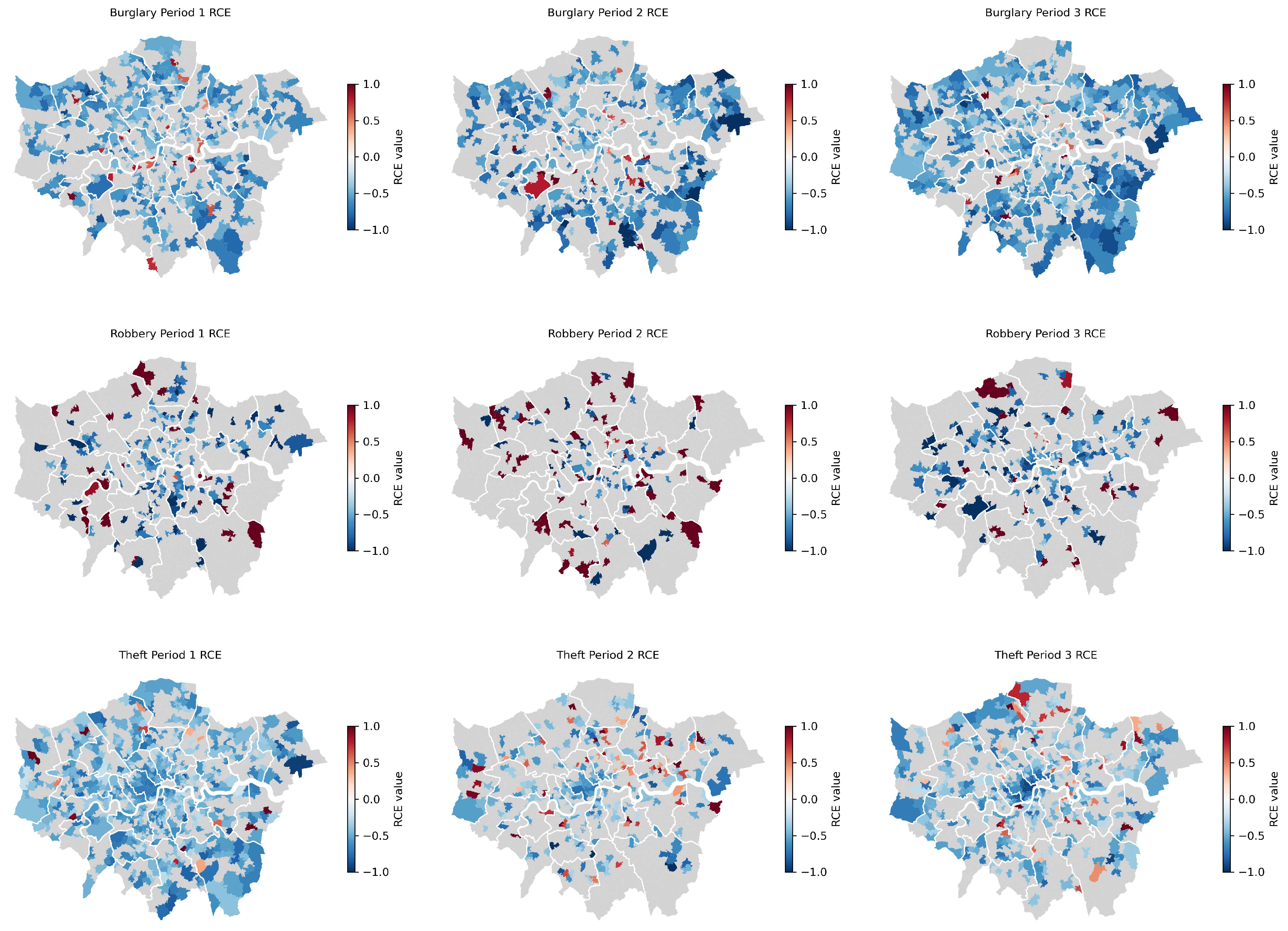
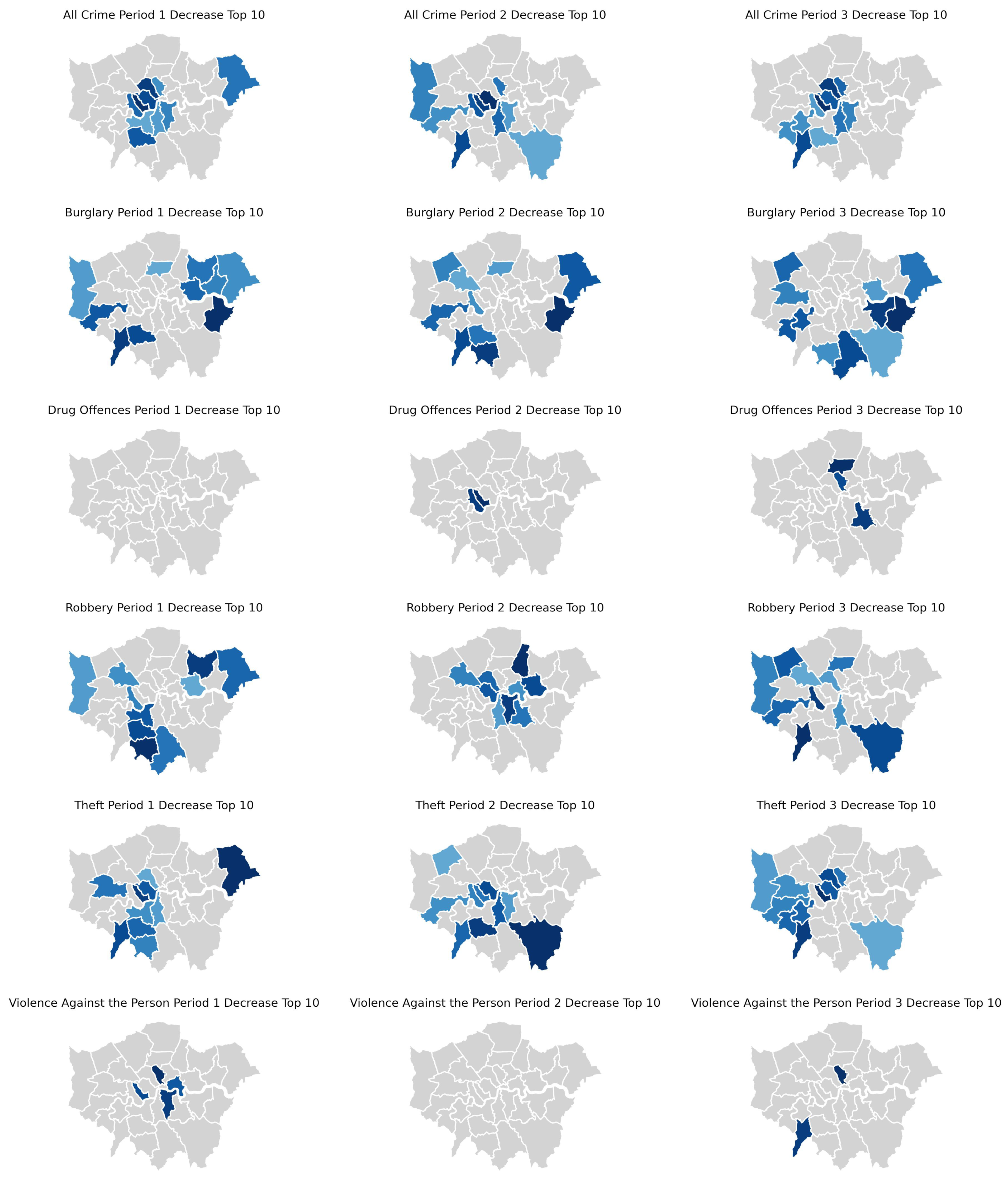
5.3.2. Analysis for Acquisitive Crimes

The outcomes of the logistic regression models for burglary during the three instances of lockdown are presented in Table 6, displaying the odds ratios (ORs) of all predictors.
Notably, during the first lockdown period, there was a significant reduction in the odds ratio risk associated with the proportion of males. According to its OR, for each unit increase in the proportion of males (normalised due to data standardisation), the risk of a significant burglary increase diminished by approximately 56% (OR = 0.44). Amid the second lockdown, the proportion of minors, population density, and the employment experience of the unemployed were the primary risk factors associated with an increase. Particularly, the latter two factors played significant roles. For each unit increase in the proportion of unemployed individuals without employment for a year, the risk of a notable burglary increase surged by a factor of 6.6 (OR = 6.6). An increase of one unit in population density translated to nearly a five-fold risk (OR = 5.1). Intriguingly, contrary to our expectations, mobility reduction only restrained the risk of burglary increase during the second lockdown, proving insignificant during the other two lockdown instances. Throughout the third lockdown, a substantial reduction in the proportion of elderly individuals markedly curbed the escalation of burglary. With each unit increase in the proportion of individuals aged 60 and over, the risk of escalation decreased by 93.6%. Furthermore, it is noteworthy that during all three lockdowns, the effectiveness of “stop and search” was not statistically significant.
In addition to the variables mentioned above, burglary’s variations displayed a robust correlation with the proportions of other crime types. Apart from the control variable “burglary ratio”, the risk of burglary demonstrated a strong positive correlation with the overall crime count. Furthermore, during the second lockdown period, regions with higher proportions of expressive crimes, such as drug offences and violence, also experienced an amplified risk of an increase in burglary.
During London’s first lockdown, a higher ratio of males in a population seemingly reduced the risk of burglary, possibly due to restrictions curtailing male offenders’ activities. However, such an effect diminished in subsequent lockdowns, owing to potential adaptations to lockdowns. In the second lockdown, a higher proportion of teenagers significantly increased the risk of burglary, coinciding with this being the only period with schools open. It also experienced increased burglary risks in areas with a higher population density and long-term unemployment, potentially due to financial strains and relaxed restrictions. Additionally, increased drug offences during this period might interactively influence an increase in burglaries. Simultaneously, the economic impacts during the first and second lockdowns was direct and profound, with the Coronavirus Job Retention Scheme (CJRS), also known as the ‘furlough’ scheme, providing support to help bridge the support gaps. By the time of the third lockdown, enhancements to the ‘furlough’ scheme had helped to provide relief to unemployment pressures, reducing the likelihood of potential offenders resorting to burglaries. Instead, during the third lockdown, a higher proportion of elderly people in the population surprisingly decreased burglary risks, who were thought to adhere more strictly to lockdown measures, enhancing household occupancy and thus preventing burglaries.
Table 7 presents the regression outcomes for robbery. It is evident that the number of variables associated with an increased risk of robbery is notably limited. This signifies that the following independent variables cannot explain the factors contributing to robbery during the lockdown period. The proportion of individuals within the unemployed category, specifically those who had not worked within the last year, emerged as the sole significant factor driving the increase in robbery during both lockdowns 1 and 2. Particularly during lockdown 1, for each unit increase in the proportion of individuals who had not worked within the last year, the risk of robbery escalation surged by nearly 3.8 times (OR = 3.8). This observation implies that economic pressures arising from the lockdown might augment criminal tendencies among the unemployed.
Furthermore, akin to burglary, during lockdown 2, the proportion of drug offences exhibited a strong positive correlation with the risk of robbery occurrence (OR = 1.5). Lastly, the reasons behind the increase in robberies during lockdown 3 remain unclear.
The increases in robberies during the initial lockdown phases appeared to be significantly correlated with the rises in long-term unemployment, a trend likely exacerbated by the economic pressures resulting from the lockdowns. However, with the continuous refinement of the ‘furlough’ scheme, this program started to see the significant easing of the financial strain on the unemployed population during the third lockdown, thereby reducing the propensity for robbery. Moreover, it is noteworthy that, during the second lockdown, the escalation in drug offences also increased the risks of robbery, suggesting that the increase in acquisitive crimes may be attributed to the rises in drug offences under the relaxed lockdown measures.
In Table 8, we delve into the regression results for theft. During lockdown 1, no variables can adequately account for the significant increase in theft. This could suggest that the marginal increase in theft within a few MSOAs during lockdown 1 might be attributed to random fluctuations. For lockdowns 2 and 3, the proportion of individuals within the employed category, specifically those who had worked within the last year, notably reduced the likelihood of theft escalation.
Additionally, during lockdown 2, the proportion of individuals aged 60 and above, and the proportion of those with reduced mobility, displayed negative correlations with the increase in theft. Intriguingly, unlike the other two acquisitive crime types, areas with higher drug ratios exhibited a lower risk of theft increase.
Initially, it was observed that the population aged over 60 exhibited a reduced risk of theft crimes, specifically during the second lockdown period. Such a reduction could be attributed to their continuing adherence to lockdown regulations and leaving home less frequently despite the relaxation of restrictions. As a consequence, it diminished their likelihood of becoming victims of thefts. Secondly, individuals without long-term unemployment showed a decreased risk of theft during the second and third lockdowns as opposed to the first lockdown. This variation may be due to the less severe economic pressures compared with the first lockdown. During later lockdowns, those who had been employed in the 12 preceding months were likely to have a more robust financial status, making them less prone to engaging in thefts. Lastly, an intriguing phenomenon was noted during the second lockdown in that areas with higher drug offences were inversely correlated with a lower risk of increased theft. This trend could be associated with the reallocation of police resources, especially following the surge in drug offences during the first lockdown, and further leading to a heightened focus on such crimes, possibly at the expense of addressing theft-related activities.

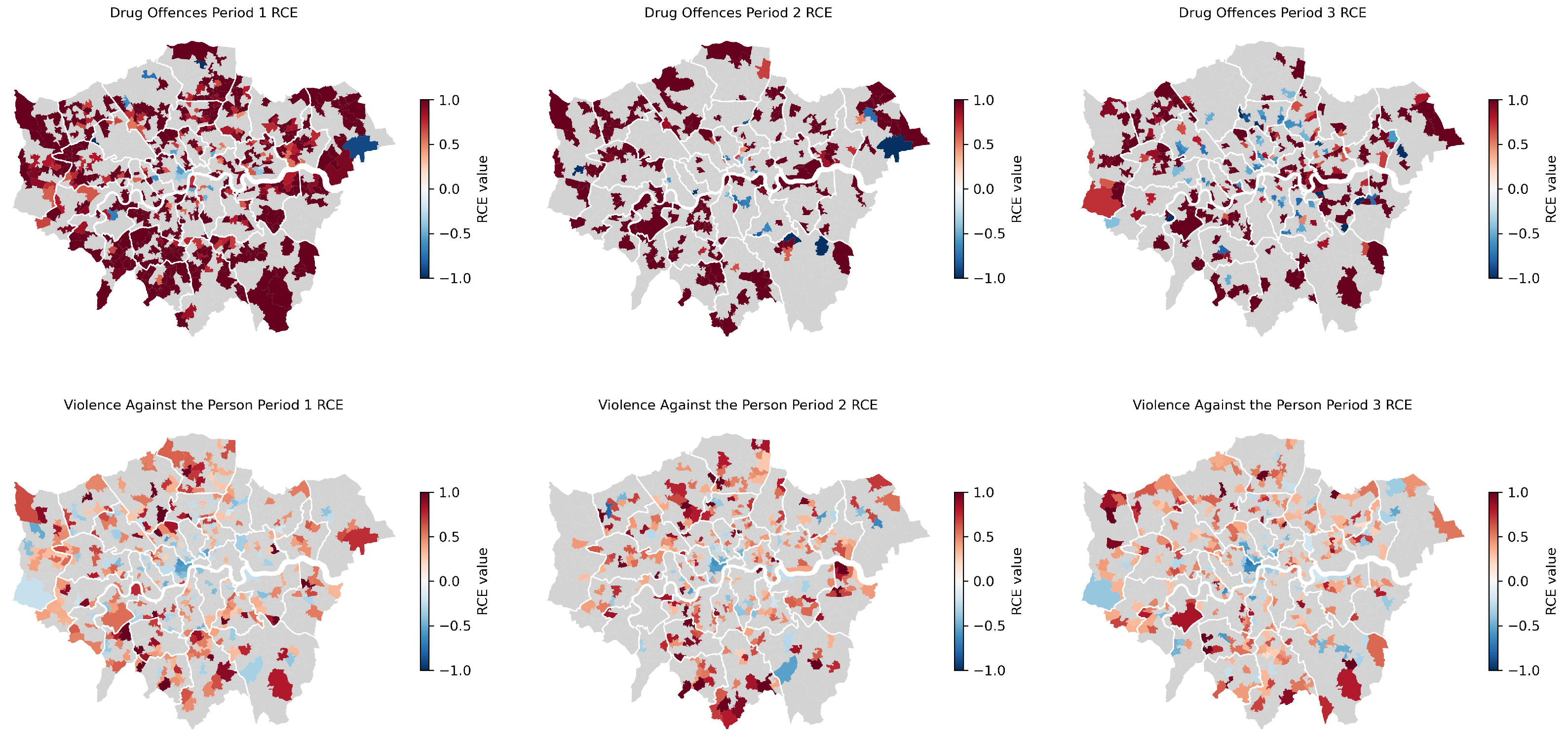
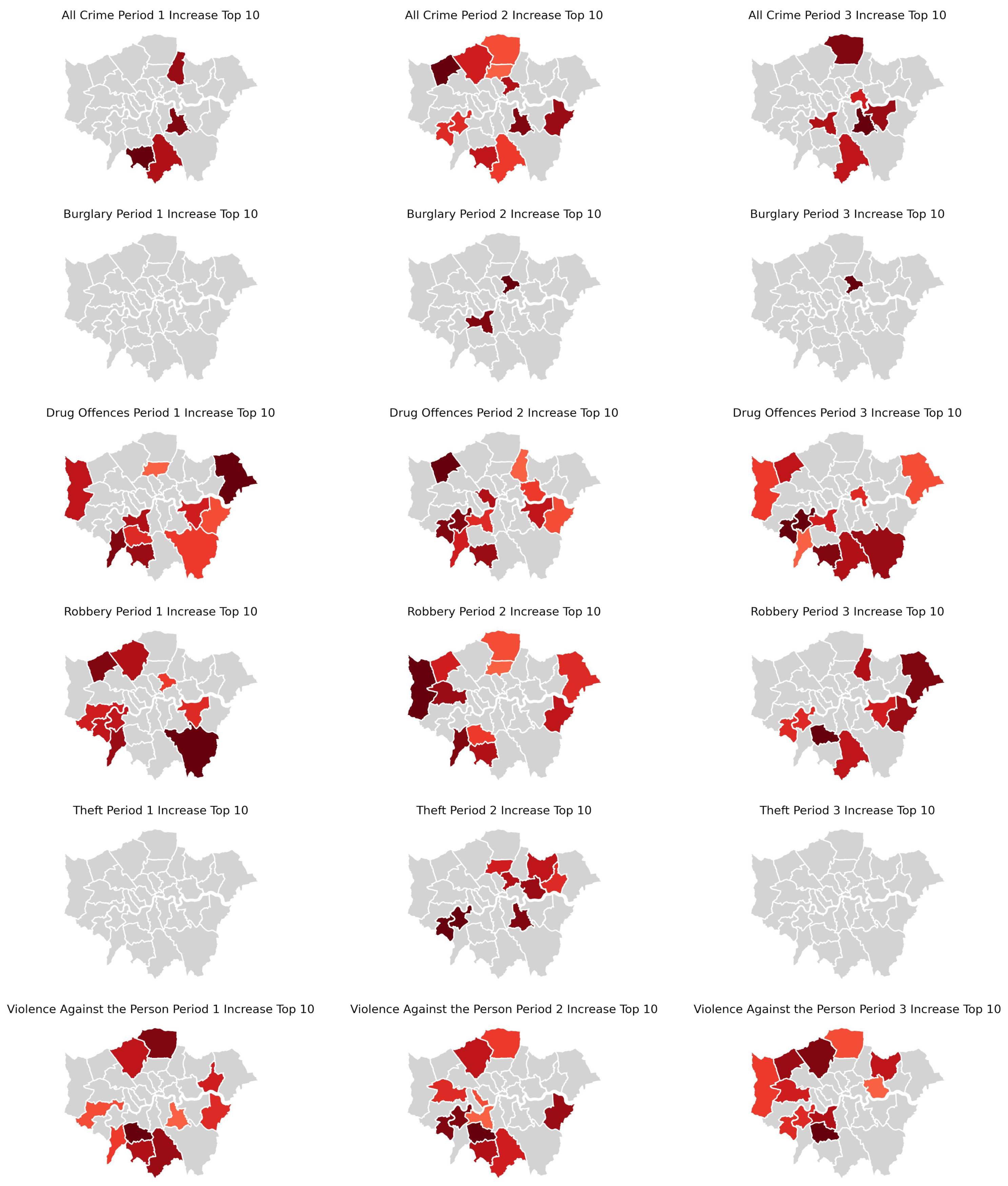
5.3.3. Analysis for Expressive Crimes

To start, Table 9 and Table 10 provided a comparison between the results of geographically weighted logistic regression (GWLR) and the global logistic regression models for expressive crimes (indicated as LR in the tables). The Akaike Information Criterion (AIC), a model selection criterion, is employed for assessment. It gauges the quality of a model in terms of both fit and complexity, preventing biased or overfit predictions [42]. A lower AIC signifies lower complexity and higher fit. The pseudo R-squared measures the goodness of fit for logistic regression models, indicating the percentage of explained variance. From the two tables, it is evident that, for both types of expressive crime, GWLR outperforms LR in terms of AIC and pseudo R-squared across all models. It is particularly noteworthy that, for drug offences during lockdown 2, the GWLR’s pseudo R-squared exceeded the LR’s by six percentage points. This demonstrates that the GWLR effectively eliminates redundant information and can better predict MSOAs with significantly increased crime.
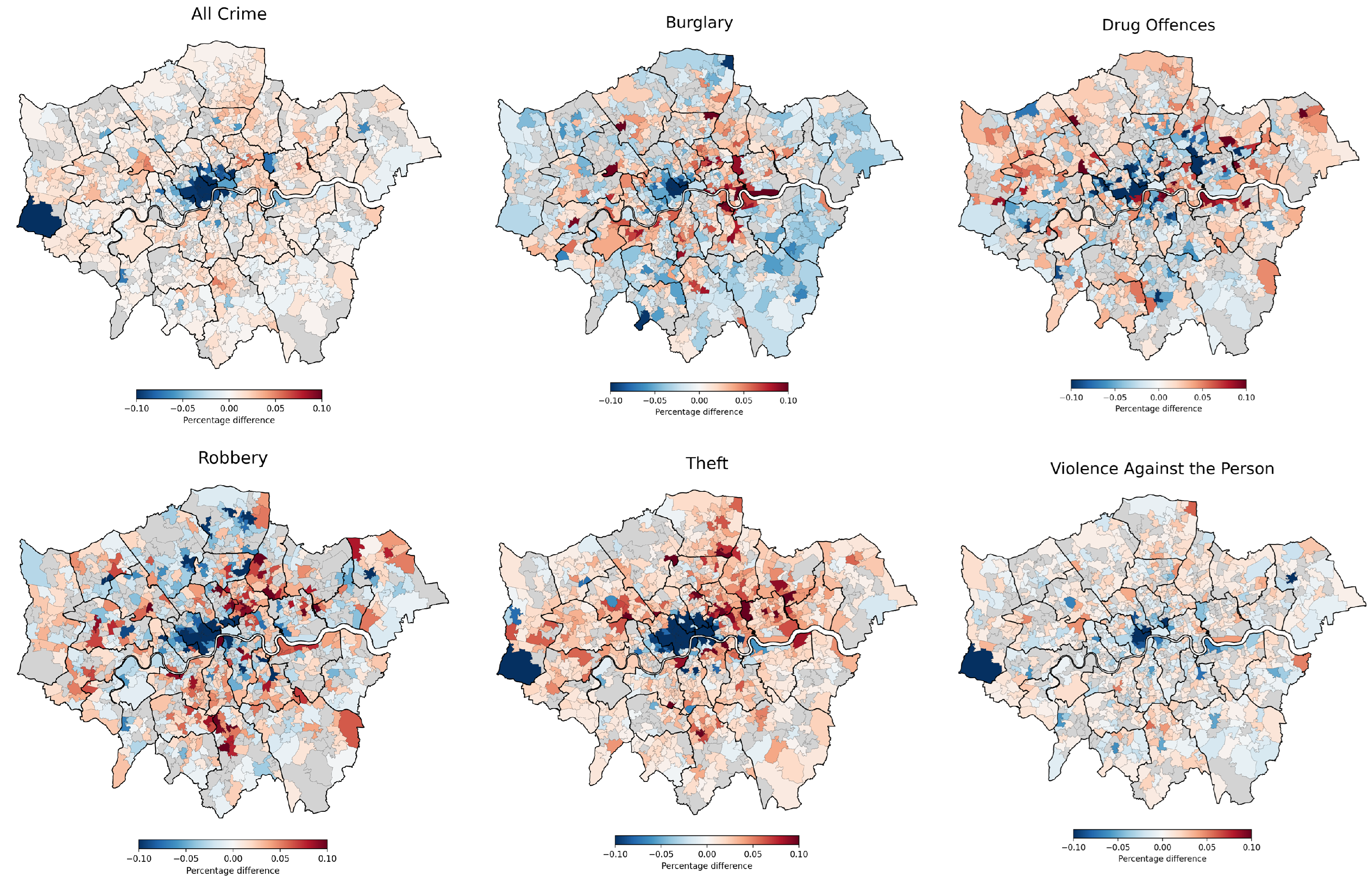
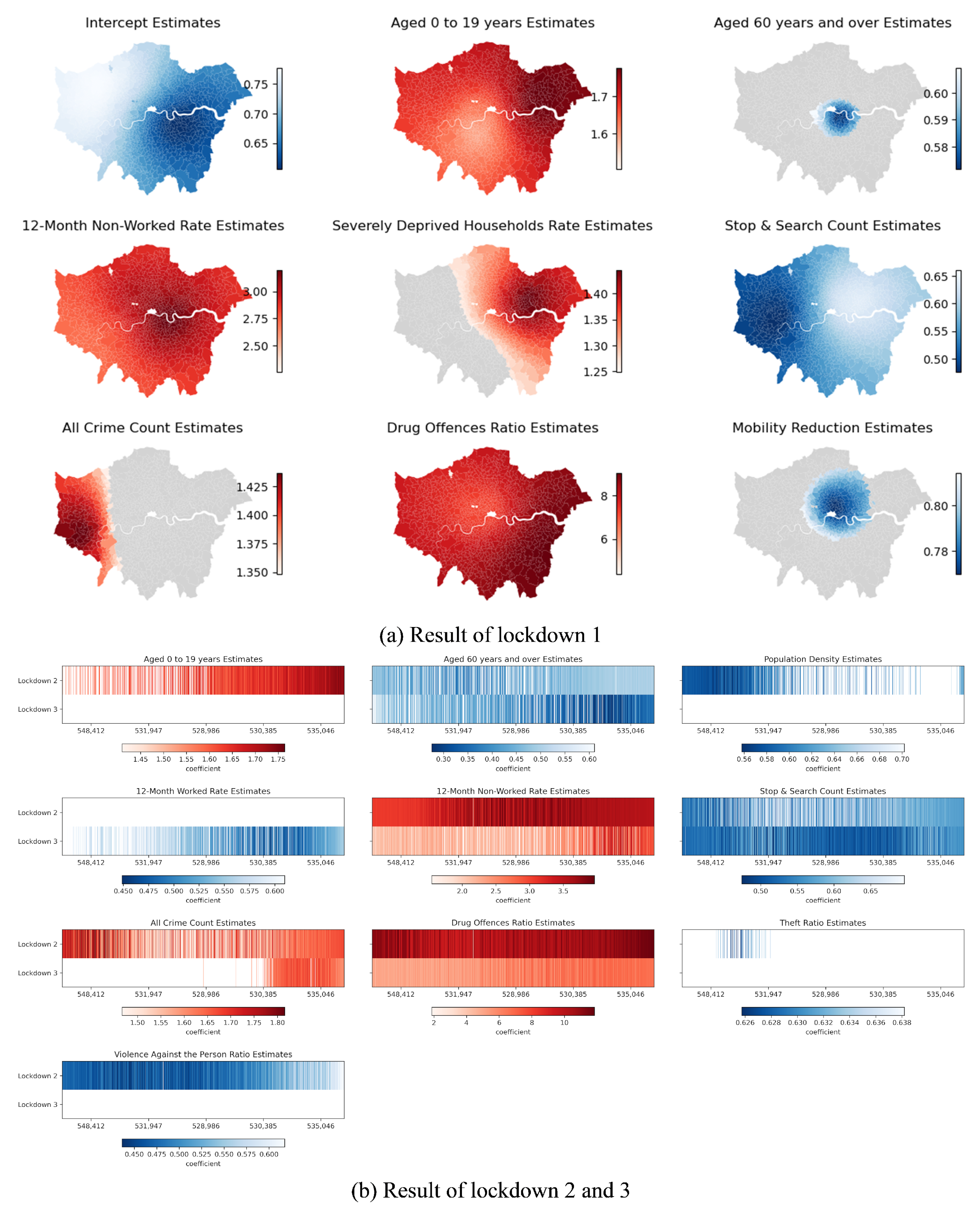
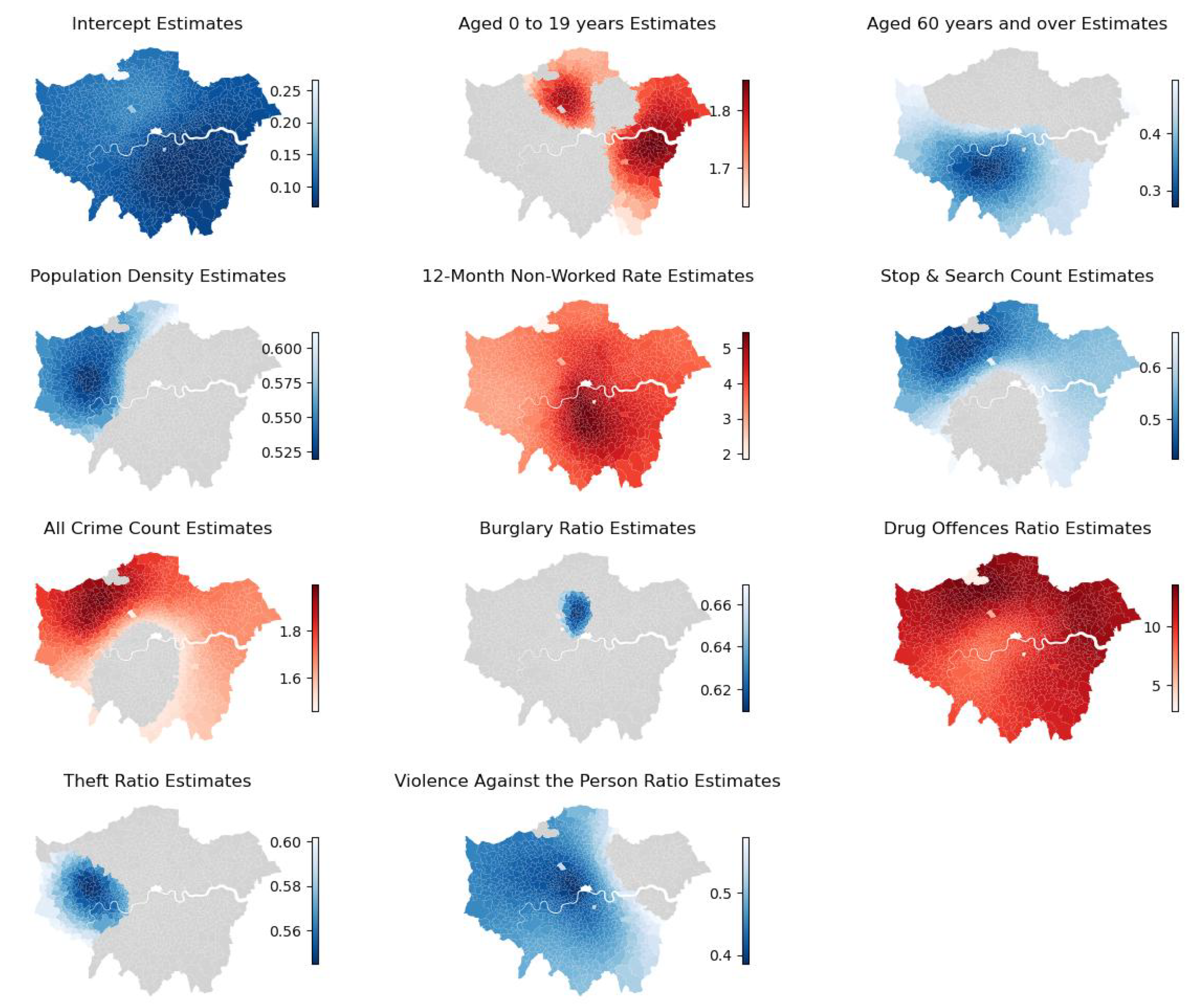
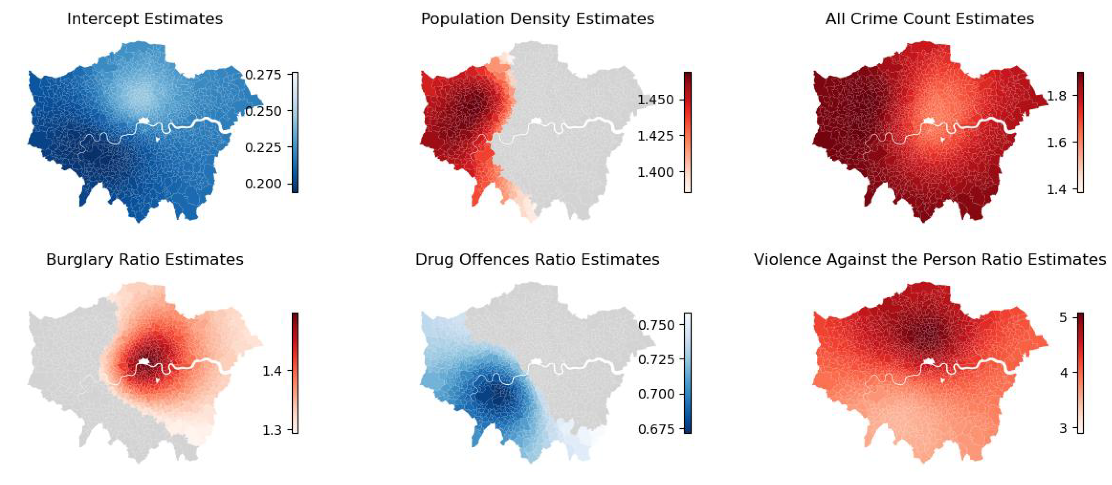
Figure 16 illustrates the GWLR results for drug offences during the three lockdown periods. This visualisation method enables us to discern how the coefficients of all explanatory variables change across the east–west direction of London during the two latter lockdowns.
The influence of the population age structure is highly significant, primarily regarding the prevalence of drug offences. During the initial two lockdowns, MSOAs with a higher proportion of individuals aged 19 and below exhibited a more pronounced increase in drug offences. In lockdown 1, the proportion of individuals aged 19 was significant for all MSOAs in London, particularly in the western and eastern peripheral areas (such as Havering and Hillingdon), with odds ratios (ORs) reaching 1.78 (see Appendix A Table A4). This implies that, for these regions, a unit increase in the proportion of underage individuals leads to a 1.78-fold increase in the risk of significant drug offences. In lockdown 2, the impact of this factor was primarily concentrated in the eastern and northern peripheral areas (e.g., Enfield and Havering). Conversely, during the latter two lockdowns, areas with a higher proportion of individuals aged 60 and above were associated with lower risks of abnormally increased crime. As depicted in Figure 16b, the positive impact of this factor, spreading from the city centre to the entirety of London, evolves as lockdowns progress.
Furthermore, similarly to acquisitive crimes, the employment history of the unemployed is also a crucial factor for drug offences. Over the three lockdowns, a strong positive correlation exists between the proportion of individuals unemployed over a year and the increase in drug offences, holding statistical significance across all MSOAs. According to Appendix A Table A4, in lockdown 1, the median odds ratio for this variable is approximately 3. This signifies that, for each unit increase in the proportion of individuals unemployed for over a year, the risk of significantly increased drug offences in that area triples. The median odds ratio for this risk factor continues to rise during lockdown 2, reaching 4, and only reduces to around 2.3 during lockdown 3. However, combined with Figure 15, it remains a significant cause for the greater number of significantly increased MSOAs in the eastern areas (Redbridge, Newham, and Tower Hamlets) during lockdown 3. Conversely, during lockdown 3, the higher the proportion of individuals unemployed for less than a year, the lower the risk of increased drug offences. Apart from the employment status, the proportion of severely deprived households acted as a risk factor for drug offences in the eastern and northern areas during lockdown 1.
Lastly, considering the crime-related factors, stop and search consistently played a proactive role in curbing the increase in drug offences throughout all three lockdowns. On average, each unit increase in stop-and-search reduces the risk of the growth in drug offences by half (see Appendix A Table A4, Table A5 and Table A6). However, the effect of stop and search in the southwestern region during lockdown 2 is not statistically significant. Moreover, similarly to acquisitive crimes, areas with higher overall crime rates are associated with greater risks of drug offence increases. Interestingly, violent crime and drug ratios in the western region exhibit an inverse relationship with the growth of the risk of drug offences.
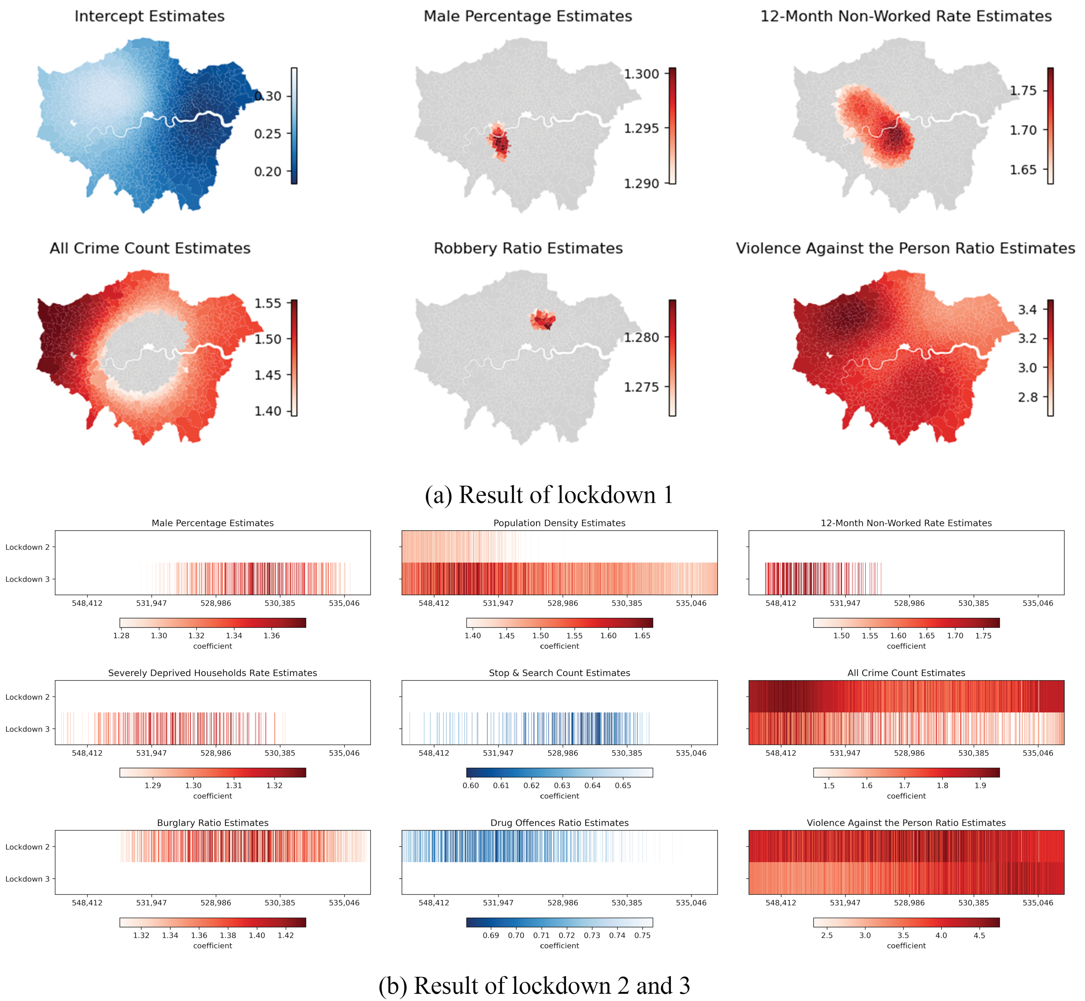
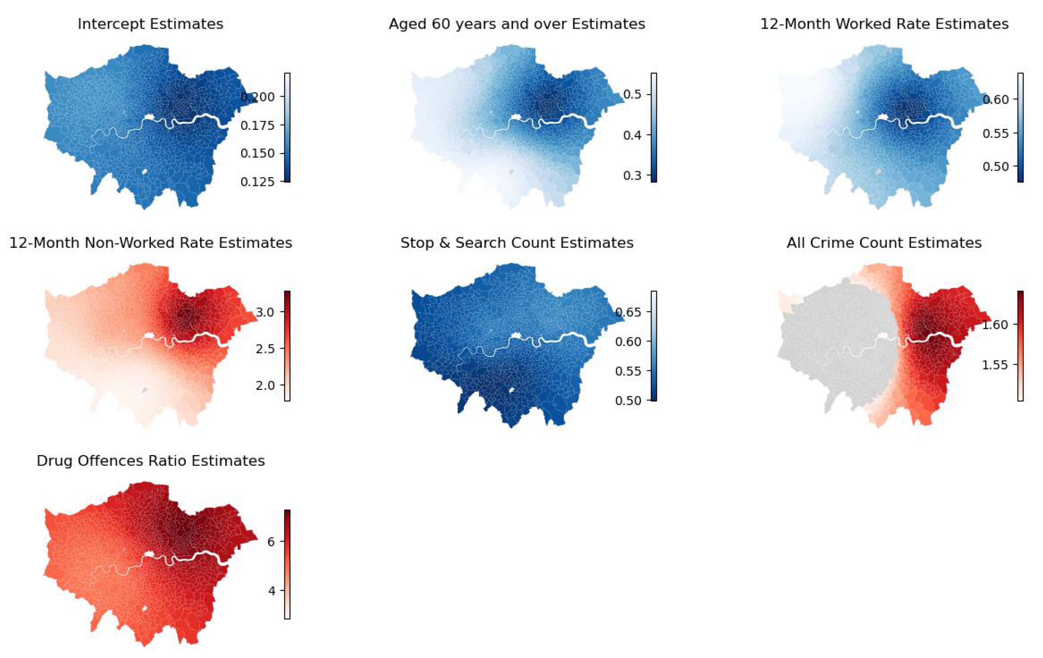
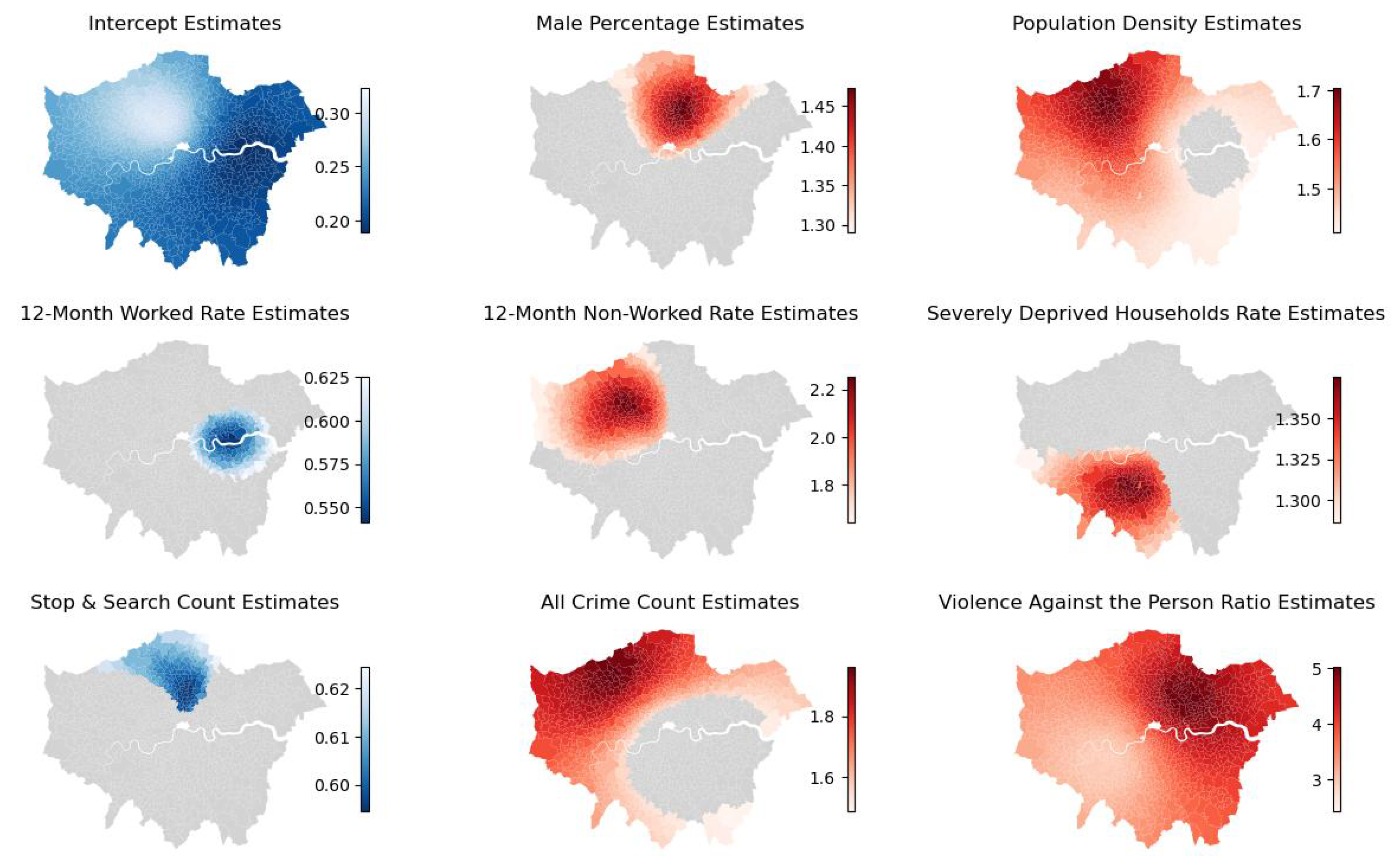
Figure 17 illustrates the GWLR outcomes for violence against persons. Firstly, an increased proportion of males is associated with a significantly elevated risk of violent crime in certain MSOAs. This phenomenon emerged near Hammersmith and Fulham as well as Wandsworth during lockdown 1. However, during lockdown 3, the impact of the proportion of males in the population is more pronounced in the northern regions (see Appendix A Figure A6). Additionally, the population density significantly increased the risk of violent crime growth during the latter two lockdowns. Notably, in the northwestern regions during lockdown 3, the risk of violent crime growth increases by approximately 1.7 times for every standard unit increase in population density. Unlike drug offences, the age structure of the population does not exhibit a significant influence.
Secondly, the employment status of the unemployed also significantly affects violent crime. However, violent crime is positively correlated with the proportion of individuals unemployed for over a year only in the western areas during lockdowns 1 and 2. Furthermore, the proportion of severely deprived households is also one of the risk factors significantly contributing to the increase in violent crime. Unlike drug offences, this situation occurred in the southwestern areas during lockdown 3 (such as Richmond, Kingston, and Sutton), whereas drug offences are associated with this factor during lockdown 1. This implies that, during the early stages of the lockdown, law enforcement should focus on drug offences in areas with a higher proportion of impoverished residents, and should later be more alert about the occurrence of violent crime in these regions.
Differing from drug offences, stop and search only played a role in reducing the risk of violent crime in the northern areas of London (e.g., Enfield, Barnet, and Haringey) during lockdown 3. Additionally, similarly to drug offences, during lockdown 2, the increased risk of violent crime in the western and southern areas of London is inversely related to the drug offences ratio. Conversely, at the intersection between Hackney and Waltham Forest during lockdown 1, as well as in the majority of MSOAs in the eastern parts of London during lockdown 2, the increased risk of violent crime is positively correlated with the robbery ratio. This implies that law enforcement needs to simultaneously pay attention to the occurrence of both of these types of crime in these areas during the restriction period.

6. Discussion

In general, there was a shift in the distribution of crime in London from the centre to the periphery in 2020. Analysing the point pattern distribution in Section 5.1 reveals a significant decrease in crime proportions within the city centre and a slight increase in the outskirts. In contrast, in Chicago, a substantial acquisitive crime cluster emerged in the city centre during 2020 [15]. This difference could be attributed to a surge in burglary and violent crime resulting from the George Floyd protests that took place in the United States in May 2020. A similar trend to that in London was observed in most Mexican cities, where crime rates experienced a more pronounced decrease in densely populated urban core areas. Aligned with the routine activity theory, this phenomenon might stem from reduced interactions between criminals and potential victims [43].
The crime hot spots in London for 2020 expanded beyond the original five central boroughs to encompass the surrounding and peripheral areas. Notably, the distribution of the two expressive crime categories underwent more significant changes compared to acquisitive crimes, leading to new crime hotspots. According to Quick’s findings, the clustering of expressive crime may be linked to the concentration of non-residential land use and residents. This aspect will be further investigated in the subsequent phases of the study [44].
From the analyses, lockdown measures produced notably significant effects on all types of crime in London, with the most substantial decrease in crime rates observed during the initial lockdown, surpassing the effects of the two subsequent lockdowns. This phenomenon effectively validates the applicability of the routine activity theory, which postulates that the occurrence of a crime represents the convergence of three elements in space and time: a motivated offender, a suitable target, and the absence of a capable guardian. Lockdown measures in London had significantly altered the routine activities of potential offenders and targets, disrupting the possibility of crucial convergence. Consequently, as individuals adapted to social distancing measures, crime patterns were anticipated to change into a more stable state; it then reflected the dynamic nature of criminal activity in response to changes in societal patterns. The results consolidated the routine activity theory’s ability to explain crime rate fluctuations during lockdowns [11].
In the context of acquisitive crimes, the majority of MSOAs experienced distinct reductions in their crime counts. Specifically, areas where theft and robbery decreased were predominantly concentrated in the city centre, while instances of reductions in burglary are more prevalent in peripheral urban regions. This phenomenon might be attributed to the sharp reduction in population mobility in the city centre, resulting in decreased criminal opportunities for theft and robbery, which necessitate interactions between offenders and victims [11,12]. Moreover, Frith et al.’s analysis establishes a significant correlation between London’s burglary rates and residential occupancy rates [45]. Given that residents in peripheral regions continued to work from home during lockdowns, daytime burglary occurrences decreased. Conversely, the higher overall housing occupancy in the city centre could account for the lack of significant change in this context.
Furthermore, areas with significant decreases in robbery were notably fewer compared to those of theft and burglary. Such an observation aligns with the findings by Campedelli et al. in Chicago, where only 2.6% of communities witnessed a significant reduction in robbery [19]. However, in contrast to the Chicago scenario, some peripheral areas in London saw significant robbery incidents increase under the influence of lockdown measures, especially during the second lockdown. This divergence prompts a further investigation in subsequent analyses.
Conversely, the restrictions have led to a considerable rise in expressive crimes across numerous MSOAs. Drug offences exhibited a particularly pronounced increase during the first lockdown. This phenomenon could be attributed to the heightened psychological and economic pressures resulting from social distancing measures [5,6,7,8,46], aligning with the explanation provided by the general strain theory. Another explanation for the abnormal increase in drug offences could be that the police resources freed up due to the reduction in acquisitive crimes during the lockdown, and were then redirected towards drug offences. Hence, although the total number of crimes increased, the actual number of cases did not changed. Correspondingly, the reduction in drug offences observed in some areas during lockdown 3 might be due to drug dealers and consumers adapting to the restrictions in developing new anti-surveillance strategies, which led to a decrease in the recorded numbers of drug offences. Additionally, the MSOAs witnessing an increase in expressive crimes are predominantly located in the peripheries of the city. This association may relate to deficient regulatory oversight and the proportion of residential land use in these areas [44]. The specific causes of this pattern will be analysed in subsequent sections, drawing upon the results of the GWLR analysis.
Regression analyses have contributed to the corroboration of numerous viewpoints within the current research landscape and aligned with the presuppositions made earlier in this paper, but also with several distinctive conclusions. Firstly, the employment history of the unemployed holds significant sway over almost all crime categories. On the one hand, individuals that were unemployed for over a year during lockdown are under considerable economic duress, markedly heightening their proclivity for engaging in acquisitive crime [5,6]. This risk factor appears to be the singular driver of the increase in robbery. On the other hand, the psychological strain arising from prolonged unemployment contributes to the risk of expressive crime, particularly drug offences. This correspondence with the general strain theory is evident. Therefore, the distinctive conclusions drawn from the regression analyses about the impact of prolonged unemployment on crime rates offer empirical support to the general strain theory. They provide real-world evidence of how economic and psychological strains can lead to an increase in certain types of criminal behaviour, thus validating the theory’s applicability in explaining crime patterns during unique societal disruptions like the COVID-19 lockdowns. Despite alleviating economic pressures on employers and employees through the JRS policy, those enduring long-term unemployment continue to confront substantial challenges [6]. Hence, augmenting financial assistance and psychological well-being support for the long-term unemployed could emerge as an effective crime mitigation measure.
Secondly, the demographic structure of the population emerged as a vital factor influencing the risk of crime escalation. MSOAs with higher proportions of youth exhibited greater risks of burglary, theft, and drug offences. Due to shifts in instructional modes and reduced social interaction with peers, the elevated academic and mental pressures on young individuals remained unaddressed. According to Lehmann et al.’s survey of adolescents, nearly 60% experienced decreased learning efficiency, with around 30% expressing concerns due to school closures [47]. Such negative emotions undoubtedly stimulate criminal actions [13]. Conversely, areas with higher proportions of residents aged 60 and above display reduced risks of burglary and drug offences growth. Fattah’s research findings offered an interpretation of the phenomenon, proposing that older individuals and those with criminal backgrounds have fewer opportunities for exposure and demonstrate increased protective awareness. Consequently, this led to notably lower victimisation rates when compared to their younger counterparts. It is crucial to recognise the possible impacts of home isolation on the elderly, including feelings of loneliness and psychological stress [48]. The reduction in population mobility during lockdown 2 indeed diminished the risk of an acquisitive crime surge, but did not significantly affect acquisitive crimes during lockdowns 1 and 3. This could be attributed to the restrictions of lockdown 2 curtailing the resurgence of theft and robbery observed after lockdown 1, yielding a significant effect.
Lastly, the effectiveness of stop and search was found be primarily confined to expressive crimes. This phenomenon could be attributed to the lower prevalence of street-level acquisitive crimes during lockdowns, diminishing the significance of stop-and-search measures. Conversely, in the case of drug offences, stop and search exerted consistently substantial effects during each lockdown. According to Halford’s investigation, the number of stop-and-search operations in the UK actually increased during the pandemic, especially to determine the possession of controlled drugs [49]. However, due to the lower effectiveness of stop and search during the lockdown compared to the same period in 2019, Halford et al. argued that stop and search did not effectively reduce the occurrence of drug offences [49]. In contrast, the GWLR model’s findings countered this finding in that stop and search significantly curbed the rise of drug offences across all areas of London during the three lockdowns. This led us to believe that stop and search not only serves as a preventive and investigative measure but also, more crucially, exerts a potent deterrent effect on both drug dealers and consumers.
Furthermore, building upon Halford et al.’s findings, it is notable that stop-and-search incidents related to theft witnessed a substantial increase. However, our results presented a contrasting result, indicating that stop and search did not significantly curb the rising trend of thefts in London, and hence verified the viewpoint that the police should exercise heightened caution when allocating police resources during lockdown periods. This enhanced stop-and-search operations directed at crimes such as robbery and violent offences, which experienced a noticeable surge during the lockdowns.

7. Conclusions

This study delved into the evolving spatiotemporal patterns of crime in London during the pandemic, analysing the impacts of three distinct lockdowns on both acquisitive and expressive criminal activities. To begin, a comparative analysis with historical data was employed to elucidate the overall alterations in crime distribution across London. This examination revealed significant changes, evident on both temporal and spatial scales, with discernible differences between the two crime categories. Temporally, acquisitive crime displayed a noteworthy correlation with the initiation and conclusion of each lockdown, exhibiting a pattern of initial decrease followed by a subsequent increase. Conversely, expressive crime consistently manifested a significant escalation during the lockdown periods. Spatially, expressive crime exhibited numerous hotspots, whereas acquisitive crime remained relatively consistent with pre-pandemic conditions. Notably, both categories witnessed a shift in their epicentres from the city centre to peripheral regions.
To enable a more precise analysis of crime variations across different periods and areas of London during the pandemic, this study innovatively incorporated the Bayesian structural time series (BSTS) model coupled with restriction-level time series to quantify the impact of three distinct lockdowns on diverse MSOAs within London.
The results indicate that the effects of the first and third lockdowns were more pronounced with regard to acquisitive crime. Notably, burglary and theft exhibited substantial declines in numerous MSOAs, albeit with spatial disparities. Regions marked by significant changes in robbery were relatively limited, with similar counts of areas witnessing noteworthy increases and decreases. For both expressive crime types, drug offences and violent offences displayed significant escalation in several peripherally located MSOAs. Over time, the number of areas characterised by substantial increases in drug offences diminished, while those experiencing a notable surge in violent crime remained consistent.
Lastly, employing logistic regression and geographically weighted logistic regression (GWLR) models, this study delved further into the factors contributing to the significant increase in crime during the pandemic. The results underscore the significant influence of the population age structure, unemployment, and law enforcement interventions on altering crime patterns during lockdown. Moreover, the interrelationships between different crime types were observed. This study emphasises the significance of the judicious allocation of law enforcement resources and enhancing unemployment-related welfare, strategies that could effectively mitigate the risks associated with increased crime during lockdown periods.

Author Contributions

Conceptualisation, Yijing Li and Rui Wang; methodology, Rui Wang and Yijing Li; software, Rui Wang; validation, Rui Wang; formal analysis, Rui Wang; investigation, Rui Wang and Yijing Li; resources, Yijing Li; data curation, Rui Wang; writing—original draft preparation, Rui Wang; writing—review and editing, Yijing Li; visualisation, Rui Wang; supervision, Yijing Li; project administration, Yijing Li. All authors have read and agreed to the published version of the manuscript.

Funding

This research received no external funding.

Data Availability Statement

The data presented in this study are available on request from the corresponding author.

Conflicts of Interest

The authors declare no conflicts of interest.

Abbreviations

The following abbreviations are used in this manuscript:
STLSeasonal and Trend decomposition Using LOESS
SPPTSpatial Point Pattern Test
BSTSBayesian Structural Time Series
LRLogistic Regression
GWLRGeographically Weighted Logistics Regression
MSOAMiddle Super Output Areas

Appendix A

Table A1. The RCE distribution of all crime and acquisitive crimes.
Crime TypePeriodDecreased MSOAs%Increased MSOAs%RCE MeanRCE MedianRCE MaxRCE Min
All crimes134.326.11−0.10−0.090.73−0.72
All crimes213.8510.29−0.01−0.020.90−0.58
All crimes327.706.52−0.08−0.080.65−0.84
Burglary136.052.34−0.33−0.371.15−0.94
Burglary230.142.44−0.30−0.352.15−1.00
Burglary345.011.63−0.36−0.412.27−1.00
Robbery114.872.85−0.30−0.3811.76−65.37
Robbery26.426.31−0.34−0.2820.23−279.40
Robbery315.892.34−0.32−0.467.79−1.00
Theft153.561.43−0.34−0.371.60−0.94
Theft220.675.70−0.13−0.192.31−1.00
Theft333.914.18−0.21−0.261.57−0.92
Table A2. The RCE distribution of expressive crimes.
Crime TypePeriodDecreased MSOAs(%)Increased MSOAs(%)RCE MeanRCE MedianRCE MaxRCE Min
Drug11.5342.360.760.6010.10−1.00
Drug21.8320.260.490.2311.03−4.53
Drug34.9919.650.290.186.04−1.00
Violence17.0324.340.140.111.48−0.59
Violence23.7723.630.180.162.13−0.79
Violence35.7024.950.150.131.68−0.71
Table A3. VIF for all variables during the different lockdowns.
VariableVIF L1VIF L2VIF L3
Aged 0–19 years2.5082.4852.526
Aged 60 years and over6.086.0676.169
Male percentage1.2781.2831.283
Population density2.6172.5862.549
12-month work rate3.473.4713.472
12-month non-work rate4.854.6854.915
Severely deprived households rate1.5411.511.519
Stop and search count2.4672.6962.769
All crimes count2.5643.1213.204
Burglary ratio1.4731.461.432
Drug offences ratio1.6311.4631.608
Robbery ratio1.2381.2391.199
Theft ratio2.2242.6772.199
Violence against the person ratio2.02.172.055
Mobility reduction1.1271.1421.142
Table A4. GWLR results for drug offences during lockdown 1 (OR).
VariableMeanSTDMinMedianMax
Intercept0.6891.0790.6060.6890.776
Aged 0–19 years1.6791.031.5051.6791.775
Aged 60 years and over0.6311.0420.5720.6330.723
Male percentage1.1541.0141.1221.1531.188
Population density0.921.0220.880.9260.951
12-month work rate0.9871.0310.9280.9871.057
12-month non-work rate2.9541.0442.2612.9653.19
Severely deprived households rate1.31.0631.1781.2971.445
Stop and search count0.5641.0930.4760.5760.66
All crimes count1.2661.0611.1471.2441.436
Burglary ratio1.0551.0420.9941.0511.143
Drug offences ratio7.9091.0734.387.8079.034
Robbery ratio0.9781.0430.9260.9671.059
Theft ratio0.8141.0260.780.8110.882
Violence against the person ratio0.9681.0450.8980.9721.044
Mobility reduction0.8191.0370.770.8160.907
Table A5. GWLR results for drug offences during lockdown 2 (OR).
VariableMeanSTDMinMedianMax
Intercept0.0991.2250.0690.1010.266
Aged 0–19 years1.6211.0991.211.6791.853
Aged 60 years and over0.4281.2290.2720.4410.766
Male percentage1.0161.0650.8631.0221.149
Population density0.6541.150.5190.6620.919
12-month work rate1.1121.1060.851.1411.3
12-month non-work rate4.0191.1681.8634.0595.458
Severely deprived households rate0.991.0570.8950.9931.09
Stop and search count0.6041.1830.4240.5950.936
All crimes count1.6021.1041.1191.5971.998
Burglary ratio0.7811.1350.610.7781.015
Drug offences ratio10.4961.1682.76210.5813.558
Robbery ratio1.0141.120.8121.0171.28
Theft ratio0.7341.2710.5450.6921.221
Violence against the person ratio0.481.1570.3860.460.788
Mobility reduction0.9191.0550.8390.9141.06
Table A6. GWLR results for drug offences during lockdown 3 (OR).
VariableMeanSTDMinMedianMax
Intercept0.1451.0790.1250.1460.221
Aged 0–19 years0.8821.050.7970.8930.977
Aged 60 years and over0.4141.2120.2820.4220.694
Male percentage1.1351.0131.1031.1391.163
Population density0.8281.0290.7980.8230.922
12-month work rate0.5491.0830.4770.5480.74
12-month non-work rate2.3121.1741.3942.2643.271
Severely deprived households rate0.9651.0630.890.9541.08
Stop and search count0.5331.0350.4990.5360.685
All crimes count1.4921.0621.1781.4921.64
Burglary ratio1.2261.0851.0441.261.351
Drug offences ratio5.8531.1342.8435.7837.257
Robbery ratio1.0741.0570.9971.0581.203
Theft ratio0.8851.0330.8270.8940.941
Violence against the person ratio0.9771.1050.8340.9671.154
Mobility reduction0.9421.1040.7850.9481.099
Table A7. GWLR results for violence against the person during lockdown 1 (OR).
VariableMeanSTDMinMedianMax
Intercept0.2441.1690.1830.250.338
Aged 0–19 years1.1041.0690.9421.1211.212
Aged 60 years and over1.2391.0741.0331.2541.374
Male percentage1.1811.0761.021.2091.301
Population density1.1171.041.0391.1211.182
12-month work rate1.1221.1010.9581.0951.359
12-month non-work rate1.4921.1491.0651.5591.779
Severely deprived households rate1.1811.0571.0611.1941.276
Stop and search count0.7391.0840.6540.730.882
All crimes count1.4261.0511.2731.4381.554
Burglary ratio1.1391.0531.0241.1511.232
Drug offences ratio0.9551.0350.8860.9491.019
Robbery ratio1.1331.0810.9881.131.284
Theft ratio0.8931.050.8370.8820.987
Violence against the person ratio3.21.0382.673.2093.463
Mobility reduction0.9111.0270.8660.9170.95
Table A8. GWLR results for violence against the person during lockdown 2 (OR).
VariableMeanSTDMinMedianMax
Intercept0.2151.0660.1940.2150.276
Aged 0–19 years0.9731.1110.7960.9911.131
Aged 60 years and over1.1581.1410.9471.1511.489
Male percentage1.1341.031.0751.1291.214
Population density1.351.0591.1631.3511.47
12-month work rate1.0881.0341.0281.0771.164
12-month non-work rate1.2661.1540.9131.3261.523
Severely deprived households rate0.9341.0210.890.940.966
Stop and search count0.7381.0380.6750.7480.876
All crimes count1.7681.0481.3841.7741.896
Burglary ratio1.3471.0541.2231.3491.496
Drug offences ratio0.7521.0620.6720.7530.876
Robbery ratio1.1771.0421.0911.1811.259
Theft ratio1.0221.2010.7331.0361.369
Violence against the person ratio4.2461.1142.8924.2465.078
Mobility reduction0.9561.0540.8580.9691.027
Table A9. GWLR results for violence against the person during lockdown 3 (OR).
VariableMeanSTDMinMedianMax
Intercept0.2371.1430.1890.2360.323
Aged 0–19 years0.9791.1070.8030.9931.157
Aged 60 years and over0.9981.1770.6891.031.267
Male percentage1.2541.0831.1211.2321.474
Population density1.5161.0541.2791.5051.706
12-month work rate0.7861.2210.5410.7951.067
12-month non-work rate1.481.2610.981.4932.25
Severely deprived households rate1.2441.0581.1351.2421.374
Stop and search count0.6581.0680.5950.6510.812
All crimes count1.5781.1171.2131.561.962
Burglary ratio1.0581.0870.9121.0471.245
Drug offences ratio0.8341.0730.7270.8450.926
Robbery ratio1.0611.0780.9261.0611.201
Theft ratio0.9791.1810.7360.9971.278
Violence against the person ratio3.7891.1812.4163.7625.033
Mobility reduction0.9091.0540.8470.8951.031
Figure A1. The 10 boroughs with the highest RCE declines. Darker colors indicate higher rankings, meaning more significant RCE decreases.
Ijgi 13 00018 g0a1
Figure A2. The 10 boroughs with the highest RCE increases. Darker colors indicate higher rankings, meaning more significant RCE increases.
Ijgi 13 00018 g0a2
Figure A3. GWLR results for drug offences during lockdown 2.
Ijgi 13 00018 g0a3
Figure A4. GWLR results for drug offences during lockdown 3.
Ijgi 13 00018 g0a4
Figure A5. GWLR results for violence against the person during lockdown 2.
Ijgi 13 00018 g0a5
Figure A6. GWLR results for violence against the person during lockdown 3.
Ijgi 13 00018 g0a6

References

  1. GOV.UK. Coronavirus (COVID-19) in the UK. 2022. Available online: https://coronavirus.data.gov.uk/ (accessed on 28 December 2023).
  2. COVID-19 Restrictions Timeseries—London Datastore. Available online: https://data.london.gov.uk/dataset/covid-19-restrictions-timeseries (accessed on 28 December 2023).
  3. ONS. GDP and Events in History: How the COVID-19 Pandemic Shocked the UK Economy—Office for National Statistics. 2021. Available online: https://www.ons.gov.uk/economy/grossdomesticproductgdp/articles/gdpandeventsinhistoryhowthecovid19pandemicshockedtheukeconomy/2022-05-24 (accessed on 28 December 2023).
  4. ONS. Unemployment Rate (Aged 16 and Over, Seasonally Adjusted)—Office for National Statistics. 2023. Available online: https://www.ons.gov.uk/employmentandlabourmarket/peoplenotinwork/unemployment/timeseries/mgsx/lms (accessed on 28 December 2023).
  5. Mayhew, K.; Anand, P. COVID-19 and the UK Labour Market. Oxf. Rev. Econ. Policy 2020, 36, S215–S224. [Google Scholar] [CrossRef]
  6. Gardiner, L. The Effects of the Coronavirus Crisis on Workers • Resolution Foundation. Available online: https://www.resolutionfoundation.org/publications/the-effects-of-the-coronavirus-crisis-on-workers/ (accessed on 28 December 2023).
  7. GOV.UK. Important Findings So Far. 2021. Available online: https://www.gov.uk/government/publications/covid-19-mental-health-and-wellbeing-surveillance-report/2-important-findings-so-far (accessed on 28 December 2023).
  8. Chandola, T.; Kumari, M.; Booker, C.L.; Benzeval, M.J. The mental health impact of COVID-19 and lockdown related stressors among adults in the UK. Psychol. Med. 2022, 52, 2997–3006. [Google Scholar] [CrossRef]
  9. Gavin, H. Acquisitive Crime. 2021. Available online: https://pure.hud.ac.uk/en/publications/acquisitive-crime (accessed on 28 December 2023).
  10. Cohn, E.G.; Rotton, J. Even criminals take a holiday: Instrumental and expressive crimes on major and minor holidays. J. Crim. Justice 2003, 31, 351–360. [Google Scholar] [CrossRef]
  11. Felson, M.; Cohen, L.E. Human ecology and crime: A routine activity approach. Hum. Ecol. 1980, 8, 389–406. [Google Scholar] [CrossRef]
  12. Brantingham, P. Patterns in Crime | Office of Justice Programs. Available online: https://www.ojp.gov/ncjrs/virtual-library/abstracts/patterns-crime (accessed on 28 December 2023).
  13. Agnew, R. Foundation for a General Strain Theory of Crime and Delinquency. Criminology 1992, 30, 47–88. [Google Scholar] [CrossRef]
  14. Abrams, D.S. COVID and crime: An early empirical look. J. Public Econ. 2021, 194, 104344. [Google Scholar] [CrossRef] [PubMed]
  15. Yang, M.; Chen, Z.; Zhou, M.; Liang, X.; Bai, Z. The Impact of COVID-19 on Crime: A Spatial Temporal Analysis in Chicago. ISPRS Int. J. Geo-Inf. 2021, 10, 152. [Google Scholar] [CrossRef]
  16. Kemp, S.; Buil-Gil, D.; Moneva, A.; Miró-Llinares, F.; Díaz-Castaño, N. Empty Streets, Busy Internet: A Time-Series Analysis of Cybercrime and Fraud Trends During COVID-19. J. Contemp. Crim. Justice 2021, 37, 480–501. [Google Scholar] [CrossRef]
  17. Paramasivan, K.; Subburaj, R.; Jaiswal, S.; Sudarsanam, N. Empirical evidence of the impact of mobility on property crimes during the first two waves of the COVID-19 pandemic. Humanit. Soc. Sci. Commun. 2022, 9, 373. [Google Scholar] [CrossRef]
  18. Campedelli, G.M.; Aziani, A.; Favarin, S. Exploring the Immediate Effects of COVID-19 Containment Policies on Crime: An Empirical Analysis of the Short-Term Aftermath in Los Angeles. Am. J. Crim. Justice 2021, 46, 704–727. [Google Scholar] [CrossRef]
  19. Campedelli, G.M.; Favarin, S.; Aziani, A.; Piquero, A.R. Disentangling community-level changes in crime trends during the COVID-19 pandemic in Chicago. Crime Sci. 2020, 9, 21. [Google Scholar] [CrossRef] [PubMed]
  20. Wang, Z.; Guo, R.; Zou, L.; Li, T.; Qiu, S. Impact of COVID-19 Outbreak on Beijing Subway Inbound and Outbound Ridership. 2023. Available online: https://www.ssrn.com/abstract=4418776 (accessed on 6 May 2023).
  21. Greater London Authority. London’s Population—London Datastore. 2021. Available online: https://data.london.gov.uk/dataset/londons-population (accessed on 8 May 2023).
  22. Census 2021 Geographies—Office for National Statistics. Available online: https://www.ons.gov.uk/methodology/geography/ukgeographies/censusgeographies/census2021geographies (accessed on 2 June 2023).
  23. Greater London Authority. Statistical GIS Boundary Files for London. 2018. Available online: https://data.london.gov.uk/dataset/statistical-gis-boundary-files-london (accessed on 8 May 2023).
  24. Metropolitan Police Serive. Recorded Crime: Geographic Breakdown—London Datastore. 2011. Available online: https://data.london.gov.uk/dataset/recorded_crime_summary (accessed on 8 May 2023).
  25. Metropolitan Police. Crime Type Definitions. 2019. Available online: https://www.met.police.uk/sd/stats-and-data/met/crime-type-definitions/ (accessed on 1 March 2023).
  26. Data Downloads | data.police.uk. 2023. Available online: https://data.police.uk/ (accessed on 1 March 2023).
  27. ONS. Census—Office for National Statistics. 2021. Available online: https://www.ons.gov.uk/census (accessed on 8 March 2023).
  28. Kadar, C.; Pletikosa, I. Mining large-scale human mobility data for long-term crime prediction. EPJ Data Sci. 2018, 7, 26. [Google Scholar] [CrossRef]
  29. Mobility Report. 2020. Available online: https://data.london.gov.uk/dataset/google-mobility-by-borough (accessed on 8 April 2023).
  30. Cleveland, R.B.; Cleveland, W.S.; Terpenning, I. STL: A Seasonal-Trend Decomposition Procedure Based on Loess. J. Off. Stat. 1990, 6, 3. [Google Scholar]
  31. Andresen, M.A. An area-based nonparametric spatial point pattern test: The test, its applications, and the future. Methodol. Innov. 2016, 9, 205979911663065. [Google Scholar] [CrossRef]
  32. Malleson, N. Andresen SpatialTest (Java). 2019. Available online: https://github.com/nickmalleson/spatialtest (accessed on 10 April 2023).
  33. Moran, P.a.P. Notes on continuous stochastic phenomena. Biometrika 1950, 37, 17–23. [Google Scholar] [CrossRef]
  34. Anselin, L. Global Spatial Autocorrelation (1). Available online: https://geodacenter.github.io/workbook/5a_global_auto/lab5a.html (accessed on 18 January 2023).
  35. Brodersen, K.H.; Gallusser, F.; Koehler, J.; Remy, N.; Scott, S.L. Inferring causal impact using Bayesian structural time-series models. Ann. Appl. Stat. 2015, 9, 247–274. [Google Scholar] [CrossRef]
  36. Larsen, K. Sorry ARIMA, but I’m Going Bayesian | Stitch Fix Technology—Multithreaded. 2016. Available online: https://multithreaded.stitchfix.com/blog/2016/04/21/forget-arima/ (accessed on 10 January 2023).
  37. Smith, T.; Haines, K. An Exploratory Study on Murders in the Chaos of COVID-19: An Analysis of Changes in Murder Rates and Patterns in Trinidad and Tobago. Int. Criminol. 2022, 2, 332–346. [Google Scholar] [CrossRef]
  38. McDowall, D.; McCleary, R.; Bartos, B.J. Interrupted Time Series Analysis; Oxford University Press: Oxford, UK, 2019. [Google Scholar]
  39. Nkeki, F.N.; Asikhia, M.O. Geographically weighted logistic regression approach to explore the spatial variability in travel behaviour and built environment interactions: Accounting simultaneously for demographic and socioeconomic characteristics. Appl. Geogr. 2019, 108, 47–63. [Google Scholar] [CrossRef]
  40. Mayfield, H.J.; Lowry, J.H.; Watson, C.H.; Kama, M.; Nilles, E.J.; Lau, C.L. Use of geographically weighted logistic regression to quantify spatial variation in the environmental and sociodemographic drivers of leptospirosis in Fiji: A modelling study. Lancet Planet. Health 2018, 2, e223–e232. [Google Scholar] [CrossRef]
  41. Shabrina, Z.; Buyuklieva, B.; Ng, M.K.M. Short-Term Rental Platform in the Urban Tourism Context: A Geographically Weighted Regression (GWR) and a Multiscale GWR (MGWR) Approaches. Geogr. Anal. 2021, 53, 686–707. [Google Scholar] [CrossRef]
  42. Burnham, K.P.; Anderson, D.R. Multimodel Inference. Sociol. Methods Res. 2004, 33, 261–304. [Google Scholar] [CrossRef]
  43. Hoehn-Velasco, L.; Silverio-Murillo, A.; de la Miyar, J.R.B. The great crime recovery: Crimes against women during, and after, the COVID-19 lockdown in Mexico. Econ. Hum. Biol. 2021, 41, 100991. [Google Scholar] [CrossRef] [PubMed]
  44. Quick, M. Exploring Crime in Toronto, Ontario with Applications for Law Enforcement Planning: Geographic Analysis of Hot Spots and Risk Factors for Expressive and Acquisitive Crimes. Master’s Thesis, University of Waterloo, Waterloo, ON, Canada, 2013. [Google Scholar]
  45. Frith, M.J.; Bowers, K.J.; Johnson, S.D. Household occupancy and burglary: A case study using COVID-19 restrictions. J. Crim. Justice 2022, 82, 101996. [Google Scholar] [CrossRef] [PubMed]
  46. Li, Y.; Zhang, Y.; Wu, Y. Frozen Cities, Frozen Crimes? Crimes changes against mobility changes following lockdowns: Case studies of London and Sydney. Pap. Br. Criminol. Conf. Online J. Br. Soc. Criminol. 2021, 20, 27–44. [Google Scholar]
  47. Lehmann, S.; Skogen, J.C.; Haug, E.; Mæland, S.; Fadnes, L.T.; Sandal, G.M.; Hysing, M.; Bjørknes, R. Perceived consequences and worries among youth in Norway during the COVID-19 pandemic lockdown. Scand. J. Public Health 2021, 49, 755–765. [Google Scholar] [CrossRef]
  48. Fattah, E.A. The Role of Senior Citizens in Crime Prevention. Ageing Soc. 1986, 6, 471–480. [Google Scholar] [CrossRef]
  49. Halford, E. Investigating the police use of stop and search in England and Wales during the coronavirus pandemic. Int. J. Law Crime Justice 2023, 74, 100617. [Google Scholar] [CrossRef]
Figure 1. Research flowchart.
Ijgi 13 00018 g001
Figure 2. The map of the studyarea used in the research. This map employs the British National Grid as the projected coordinate system, with meters as the unit for its coordinate axes. The geographical units depicted in the map are the Middle Super Output Areas of London (MSOAs).
Ijgi 13 00018 g002
Figure 3. Temperature and holiday time series: (a) the blue curve represents the time series of daily minimum temperatures, while the orange curve represents the time series of daily maximum temperatures; and (b) the blue curve represents the number of bank holidays for each month.
Ijgi 13 00018 g003
Figure 4. Example of BSTS counterfactual prediction [37].
Ijgi 13 00018 g004
Figure 5. Time series of the total number of crimes.
Ijgi 13 00018 g005
Figure 6. Time series of the number of different types of crimes.
Ijgi 13 00018 g006
Figure 7. Decomposition results of crime number time series. Each of the subplots: (a) all crime; (b) burglary; (c) drug offences; (d) robbery; (e) violence against the person; (f) theft, includes three components: trend, season, and residual.
Ijgi 13 00018 g007
Figure 8. Differences in space point patterns between 2019 and 2020.
Ijgi 13 00018 g008
Figure 9. London crime LISA clustering results for 2019 and 2020.
Ijgi 13 00018 g009
Figure 10. Changes in the trend of the number of crimes during Lockdown 1. Subplot (a) displays counterfactual prediction and actual crime count curves. Subplot (b) shows changes in the difference between counterfactual prediction and actual crime count. Subplot (c) illustrates changes in the percentage of the difference between counterfactual prediction and actual crime count relative to the actual crime count 1.
Ijgi 13 00018 g010
Figure 11. Changes in the trend of the number of crimes during Lockdown 2. Subplot (a) displays counterfactual prediction and actual crime count curves. Subplot (b) shows changes in the difference between counterfactual prediction and actual crime count. Subplot (c) illustrates changes in the percentage of the difference between counterfactual prediction and actual crime count relative to the actual crime count 2.
Ijgi 13 00018 g011
Figure 12. Changes in the trend of the number of crimes during Lockdown 3. Subplot (a) displays counterfactual prediction and actual crime count curves. Subplot (b) shows changes in the difference between counterfactual prediction and actual crime count. Subplot (c) illustrates changes in the percentage of the difference between counterfactual prediction and actual crime count relative to the actual crime count 3.
Ijgi 13 00018 g012
Figure 13. Relative cumulative impact of the lockdowns on all crime across MSOAs.
Ijgi 13 00018 g013
Figure 14. Relative cumulative impact of lockdowns on acquisitive crime across MSOAs.
Ijgi 13 00018 g014
Figure 15. The relative cumulative impact of lockdowns on expressive crime across MSOAs.
Ijgi 13 00018 g015
Figure 16. GWLR results for drug offences during the three lockdowns. (a) shows odds ratio spatial distribution during the first lockdown. Red indicates variables amplifying its impact (odds ratio > 1), while blue suggests reduced risk (odds ratio < 1). Gray denotes statistical insignificance. (b) presents odds ratios during the second and third lockdowns. Blue and red shades mirror (a), white signifies insignificance. The vertical axis represents lockdown periods, and the horizontal axis MSOA centroids’ east-west coordinates in EPSG:27700.
Ijgi 13 00018 g016
Figure 17. GWLR results for violence against the person during the three lockdowns. (a) shows odds ratio spatial distribution during the first lockdown. Red indicates variables amplifying its impact (odds ratio > 1), while blue suggests reduced risk (odds ratio < 1). Gray denotes statistical insignificance. (b) presents odds ratios during the second and third lockdowns. Blue and red shades mirror (a), white signifies insignificance. The vertical axis represents lockdown periods, and the horizontal axis MSOA centroids’ east-west coordinates in EPSG:27700.
Ijgi 13 00018 g017
Table 1. Definition of the crime types in this study.
Crime TypesDefinition
Acquisitive
crime
BurglaryThis category is the offence of unauthorised entry into a building for the purpose of burglary or attempted burglary.
RobberyThis category refers to the illegal acquisition of another person’s property by means of violence or threats. However, snatch theft is not included here.
TheftThis category covers the illegal taking of property from a person, motor vehicle, bicycle, residential or non-residential property. It also covers the storage and transaction of property after the theft has taken place.
Expressive
crime
Drug offencesThis category refers to the offence of buying, using and selling illegal drugs.
Violence against the personThis category includes a range of violent offences against the physical integrity and dignity of others from minor harassment to serious murders.
Table 2. BSTS pre-intervention and post-intervention period.
 Pre-Intervention PeriodPost-Intervention Period
Lockdown 1March 2011–February 2020March 2020–May 2020
Lockdown 2March 2011–October 2020November 2020–December 2020
Lockdown 3March 2011–December 2020January 2021–March 2021
Table 3. Global similarity index of different year groups.
 2017 vs. 20182018 vs. 20192019 vs. 2020
All crimes0.260.220.14
Burglary0.280.280.27
Drug offences0.310.280.29
Robbery0.290.280.28
Theft0.280.260.16
Violence0.310.320.26
Table 4. Global Moran’s I for different types of crime in 2019 and 2020.
 Moran’s I in 2019Moran’s I in 2020
All crimes0.440.41
Burglary0.460.44
Drug offences0.410.42
Robbery0.430.42
Theft0.450.41
Violence0.330.34
Table 5. Global Moran’s I of the residual of logistic regression models.
 Lockdown 1Lockdown 2Lockdown 3
Burglary0.0120.0360.062 **
Drug offences0.039 *0.088 ***0.057 **
Robbery−0.0010.036−0.003
Theft−0.015−0.0020.008
Violence0.092 ***0.077 ***0.050 **
Sig. codes: 0 “***” 0.001 “**” 0.01 “*” 0.05.
Table 6. Global logistic regression model for burglary.
Odds Ratio for PredictorsLockdown 1Lockdown 2Lockdown 3
Aged 0–19 years1.3543.019 **0.741
Aged 60 years and over0.5590.5030.064 **
Male percentage0.439 **0.6801.117
Population density1.6525.094 ***1.265
12-month work rate1.0181.1100.361
12-month non-work rate0.4006.606 **0.997
Severely deprived households Rate0.4581.5191.244
Stop and search count1.0500.6160.536
All crimes count2.392 **3.333 **3.991 **
Burglary ratio5.859 ***8.750 ***12.256 ***
Drug offences Ratio1.3472.705 **0.511
Robbery ratio0.4500.8651.202
Theft ratio0.5301.5220.905
Violence against the person ratio0.8772.863 *2.268
Mobility reduction1.0660.446 **0.905
Pseudo R20.46960.32810.4005
Sig. codes: 0 “***” 0.001 “**” 0.01 “*” 0.05.
Table 7. Global logistic regression model for robbery.
Odds Ratio for PredictorsLockdown 1Lockdown 2Lockdown 3
Aged 0–19 years1.4741.5200.938
Aged 60 years and over0.6780.6511.332
Male percentage1.4830.8950.862
Population density0.8430.8120.855
12-month work rate0.5180.5590.676
12-month non-work rate3.831 *3.133 **1.733
Severely deprived households rate1.4291.1530.944
Stop and search count0.5651.0020.626
All crimes count1.7881.3141.383
Burglary ratio1.1831.1210.630
Drug offences ratio1.2071.486 *1.068
Robbery ratio5.403 ***7.448 ***3.762 ***
Theft ratio0.5581.0970.985
Violence against the person ratio1.3281.4431.397
Mobility reduction1.4861.2550.771
Pseudo R20.40050.41710.3444
Sig. codes: 0 “***” 0.001 “**” 0.01 “*” 0.05.
Table 8. Global logistic regression model for theft.
Odds Ratio for PredictorsLockdown 1Lockdown 2Lockdown 3
Aged 0–19 years1.6771.0471.156
Aged 60 years and over0.2620.318 **0.573
Male percentage1.2570.9421.022
Population density0.6580.8481.284
12-month work rate0.2670.388 **0.339 **
12-month non-work rate2.4380.8290.925
Severely deprived households rate1.2040.7901.013
Stop and search count1.0470.9190.512
All crimes count0.4840.6661.206
Burglary ratio0.4150.9671.142
Drug offences ratio0.8240.550 *0.930
Robbery ratio0.6050.9120.905
Theft ratio3.869 **3.916 ***3.287 ***
Violence against the person ratio1.0121.4611.207
Mobility reduction0.8400.710 *0.894
Pseudo R20.31710.21540.1886
Sig. codes: 0 “***” 0.001 “**” 0.01 “*” 0.05.
Table 9. Comparison between the logistic model and GWLR for drug offences.
 AIC (LR)AIC (GWLR)Pseudo R2 (LR)Pseudo R2 (GWLR)
Lockdown 1931.3926.10.320.35
Lockdown 2617.6605.70.410.47
Lockdown 3753.7747.60.260.30
Table 10. Comparison between the logistic model and GWLR for violent crime.
 AIC (LR)AIC (GWLR)Pseudo R2 (LR)Pseudo R2 (GWLR)
Lockdown 1930.0917.30.180.22
Lockdown 2890.3883.80.200.23
Lockdown 3909.0849.00.210.25
Disclaimer/Publisher’s Note: The statements, opinions and data contained in all publications are solely those of the individual author(s) and contributor(s) and not of MDPI and/or the editor(s). MDPI and/or the editor(s) disclaim responsibility for any injury to people or property resulting from any ideas, methods, instructions or products referred to in the content.

