1. Introduction
The available geospatial data is increasing steadily. Distributed data collection technologies such as sensor networks, crowdsourcing and other data sources in the context of the Intent of Things (IoT), gather continuous real-time data of our environment [
1,
2]. These data are often provided as data streams and, therefore, can be processed in a streaming environment as well. This opens up opportunities to process these geodata continuously and instantaneously and gain immediate insights into processes in our environment in the same way. Furthermore, these geodata streams nowadays provide high spatial and temporal resolution and allow for sophisticated spatiotemporal analyses. These include geostatistical methods to investigate spatial and spatiotemporal processes and assess detected patterns statistically. Thereby a large amount of collected data is needed to achieve reliable statements of these statistical approaches. For this reason, the growth of spatial big data leads to a corresponding increase in application possibilities of spatial analysis algorithms such as these geostatistical analysis methods [
3]. Especially regarding real-time data including various traffic and environmental parameters gathered from our environment. An intensively applied and refined geostatistical method is the spatial and spatiotemporal autocorrelation, respectively [
4,
5]. It can be used for the exploratory investigation of spatial data, searching for patterns that differ from random processes and, thus, detecting possible mechanisms behind observed phenomena.
At the same time, we see promising developments in processing and analysis tools for streaming data. Distributed stream processing, in particular, offers opportunities to process and analyze big data in real time while applying complex calculations to the data. In our previous study [
6], we presented a methodology to adapt an extended spatiotemporal Moran’s I index originally presented by Gao et al. [
7], as a distributed streaming process. In this way, this index as a measure for spatiotemporal autocorrelation, can be applied to time series data retrieved from geodata streams. This allows for a calculation of spatiotemporal autocorrelation and its assessment using parallel permutation tests in real time.
This approach of spatiotemporal autocorrelation directly applied to geodata streams incorporates the potential to transfer real-time access to spatial big data via the IoT into a real-time analysis with similarly high temporal resolution. Such an analysis approach can intensively improve the way we derive geospatial knowledge from data on our environment. These new processing and calculation possibilities demand a new way to set up and use the spatiotemporal autocorrelation itself. Thus, instead of retrospective analyses based on historical data alone, an additional investigation with high temporal resolution is of interest. This leads to our concept of a high-frequent dynamic autocorrelation, which we intensively evaluate in this study. The resulting high-frequent dynamic autocorrelation is different from the original approach since we do not generate a single autocorrelation index for the accumulated data, but we obtain a continuous progression of the autocorrelation with high update frequency and very low latency. This allows for immediate observation of potential trends in the autocorrelation and therefore the spatio-temporal behavior of the monitored process itself. In parallel, test statistics based on permutation tests are produced with the same temporal resolution to allow for a continuous statistical assessment of the progressing autocorrelation.
This raises the question of which insights can be gained by a high-frequent dynamic variant of the spatiotemporal autocorrelation compared to conventional approaches and, furthermore, to what extent the analysis results are comparable to known methods for the analysis based on historical data. This study examines these questions. Furthermore, it investigates the influences of the chosen temporal criteria on the analysis results, which are of particular interest in such a dynamic and temporally high resolved approach. To do so, the new concept is applied to mobility data collected in New York City in 2018 [
8]. Multiple progressions of the spatiotemporal autocorrelation in the data are produced. The spatially and temporally high resolved mobility data allows for updates in rates of a few minutes while comprising time series data from multiple hours. The innovation of the presented approach is the high-frequent dynamic use of spatiotemporal autocorrelation with an extended Moran’s I index. In this context, this work includes the following novelties:
High-frequent dynamic spatiotemporal autocorrelation approach;
Geostatistical analysis in real time that adds to existing analyses based on historical data;
Immediate assessment of temporal trends and fluctuations regarding the spatiotemporal autocorrelation;
Possibility to gain insights in spatiotemporal big data in real time and analyze spatiotemporal processes while they are ongoing.
In this work, we present an evaluation study of a high-frequent dynamic spatiotemporal autocorrelation. The background and related works regarding this concept are described in
Section 2. The evaluation methodology used in this study is described in
Section 3. The results of the evaluation are presented in
Section 4 and discussed in
Section 5, with our conclusions provided at the end of the paper.
2. State of the Art and Related Work
In this section, we present the important background for this work. First, we summarize relevant literature concerning the processing and analysis of spatial streaming data. This is followed by a brief overview of the concepts and approaches for spatial and spatiotemporal autocorrelation. After that, an explanation of the extended spatiotemporal Moran’s I developed by Gao et al. (2019) [
7] is given. At last, we present our adaption of this extended spatiotemporal Moran’s I as a streaming process which was used for the study in this paper.
2.1. Related Work in Processing and Analysis of Spatial Streaming Data
Multiple suggestions for real-time geostatistical approaches in the context of the IoT can be found in the scientific literature. Cheng et al. (2012) conducted a study of spatiotemporal autocorrelation in road traffic networks in London [
9]. A study of inner-city air quality applying spatiotemporal regression on environmental data from distributed sensor networks was presented by van Zoest et al. (2020) [
10]. Both suggested that the implementation of the geostatistical analyses used as applications in near real-time is a promising further development. A method for producing air quality maps based on high temporal resolution data streams from sensor networks using geostatistical methods was developed by Schneider et al. (2017) [
11].
The analysis of streaming spatial data has been tackled in many studies. Most of these studies emphasize the gathering, filtering, and handling of geodata, which are collected from continuous data sources. In this context, Lorkowski and Brinkhoff (2015) introduced a system designed to filter, process, interpolate, observe, and store data streams from sensors utilizing a particularly efficient kriging method [
12]. It facilitates the timely recalculation of kriging calculations by working only on specific regions where the variance in the new data grid is significantly reduced. Hwang et al. (2013) presented a methodology for near real-time aggregation of georeferenced social media data [
13]. The aim was to provide a continuous source for spatiotemporal analytical methods. Laska et al. (2018) conducted a case study on spatiotemporal data streams in stream processing environments [
14]. By integrating IoT data streams into open-source tools, they implemented a state-of-the-art map matching algorithm in a distributed manner. Zhong et al. (2016) worked on improving ordinary kriging interpolator performance in a streaming environment, significantly reducing calculation time for spatiotemporal interpolation [
15].
These studies enhance the field of processing and analysis of spatial streaming data and emphasize the relevance of real-time applications of geostatistical methods. Nevertheless, an investigation of continuously calculated spatiotemporal autocorrelation and the corresponding abilities to analyze spatiotemporal processes in a geostatistical manner in real time, is still missing. The work in this paper examines the potential, behavior, and limits of an extended Moran’s I index adapted as a streaming process. In this way, our paper contributes to the field of spatial analysis in real time and presents a study on a high-frequent autocorrelation approach applied to spatial big data.
2.2. Spatial and Spatiotemporal Autocorrelation
Originally spatial autocorrelation statistics have been developed to identify a theoretical condition in which there is no spatial autocorrelation. However, in current practice, these statistics are also used to measure the degree of spatial autocorrelation present in georeferenced data [
4]. As a result, the application of these methods is no longer limited to hypothesis testing. Rather, they are applied to exploratory investigation. In this way, it is possible to examine geospatial data for patterns that indicate phenomena and processes that have previously gone undetected and are not the result of random processes.
Since the first investigations regarding spatial autocorrelation, various measures for its mathematical description have been developed. In the context of this study, the following indices were used: the classic Moran’s I introduced by Moran (1950), the local Moran’s I presented by Anselin (1995) and an extended spatiotemporal Moran’s I developed by Gao et al. (2019) [
7,
16,
17]. Some other common measures of spatial autocorrelation are Geary’s C [
18], the cross-product statistic
[
19], Getis and Ord’s G [
20], Ripley’s K [
21], Ord and Getis’ O [
22] and Matheron’s
[
23].
The extended Moran’s I index by Gao et al. (2019) was developed specifically to analyze mobility data [
7]. This index measures the deviations between time series data at different localities and determines the spatial autocorrelation in these deviations. Some other indicators for spatiotemporal autocorrelation use different approaches to integrate the temporal behavior of the examined process. One approach presented by Liu et al. (2015), is to measure spatial autocorrelation in vectors, rather than scalar values [
24]. However, this method is only suitable for static data and is unsuitable for extensive spatially and temporally resolved mobility data [
7]. Considering the temporal dimension in the weights matrix is also a possibility, as conducted in the approaches of Dubé and Legros (2013) and Lee and Li (2017) [
25,
26]. However, in these methods, the spatial observations and temporal values are considered separately [
7]. An extension of the Moran coefficient by the Pearson correlation coefficient was presented by Porat et al. (2012) [
27]. This procedure assumes a normal distribution and linear dependence of the variables. However, these assumptions cannot always be satisfied for mobility data [
7].
2.3. Extended Spatiotemporal Moran’s I
Mobility data have not only spatial but also temporal characteristics. In principle, these data can be seen as spatially distributed time series. Therefore, the deviations between individual spatially distributed values are no longer compared, as is performed in the classic Moran’s I, but the deviations between time series of values. The similarity of two time series is described by Gao et al. (2019) in two parts [
7]. This is achieved first using the temporal similarity of the trend development of the time series and second by the magnitude deviation. The temporal similarity of the trend development is estimated by a temporal correlation coefficient of two time series. The magnitude deviation is evaluated by the difference in the accumulated volumes of the two time series. Consequently, the deviation is first measured by the difference of the cumulative volumes of two time series and then adjusted for the temporal dissimilarity. To determine the temporal dissimilarity of the trend development of the time series, an adaptive temporal dissimilarity measure that covers both temporal correlation and data distance is used [
28]. The extended global (
) and local (
) Moran’s I indices are, respectively, defined as follows:
Equation (
1) shows the global (
) and local (
) extended Moran’s I indices, where
W is the spatial weight matrix,
N the number of localities and
and
are the deviations between the time series at locations
i and
j from the series of mean values. The superscript
T in
,
as well as
and
indicate, that these values are calculated over the length
T of the time series. This means the deviations
and
represent a measure of deviation in temporal trend and cumulative volume between a times series of length
T at the location
i or
j and the time series consisting of the mean values of all locations in the study area. The global and local indices
and
measure the spatiotemporal autocorrelation within time series of length
T, respectively. The global extended Moran’s I index
indicates the presence of spatiotemporal autocorrelation within the whole data set. The local indices
estimate the associated impact of individual local values.
2.4. Extended Spatiotemporal Moran’s I as a Streaming Process
In our previous study, we adapted the extended Moran’s I by Gao et al. (2019) as a distributed streaming process [
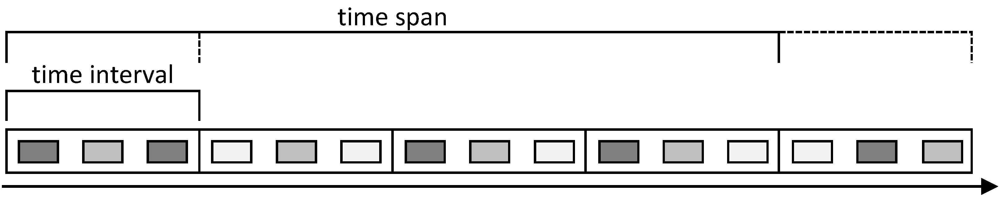
7]. For this purpose, special time semantics have been introduced. These time semantics are of particular importance for the interpretation of the result of this study. The temporal configuration of the streaming process is closely linked to the temporal configuration of the spatiotemporal autocorrelation. Two parameters are used: the time interval and the time span. These two parameters define the way the time series data is mapped to time windows inside the streaming engine. The time interval defines the step size for the calculation and therefore the time slot over which the events are accumulated and the update frequency of the result values at the same time. The time span defines the time slot over which the autocorrelation is calculated and, therefore, the data total that is considered. The relation of time interval and time span is illustrated in
Figure 1.
The introduced time interval and time span are key elements of our adaption of the approach by Gao et al. (2019) as a streaming process [
7]. Gao et al. (2019) designed their method to be applied to a large set of accumulated data in its entirety [
7]. In their scenario, the time series extends over the entire period over which the data was accumulated. In this way, a spatiotemporal autocorrelation for the whole period is obtained. In our streaming adaption, the period over which the autocorrelation is calculated shifts continuously and corresponds to the defined time span. By doing so, the calculated autocorrelation can be updated with a high frequency, incorporating new arriving data from the data stream. The time interval is used to discretize the incoming data tuples into time windows of fixed length. This defines the temporal lag between the elements within a time series. Since the original method by Gao et al. (2019) [
7] is applied to a finite data set with fixed time boundaries, it is only suitable for retrospective analyses of historical data. Our adaption as a streaming process in Lemmerz et al. (2023) on the other hand, allows for a continuous application on endless and current data streams [
6].
Another important definition from the previous study is the check values. These check values
and
are used to assess the reliability of the continuous calculation processes [
6]. A detailed description of the check values is given in
Section 3.3, where the threshold values for
and
are defined.
3. Evaluation of the Dynamic Spatiotemporal Autocorrelation
Fundamental for an evaluation of the calculated results with respect to their geostatistical meaning is that there is no generally valid ground truth to which these results could be compared. For this reason, the evaluation focuses on the question of to what extent a continuous and high-frequent calculation of the extended Moran’s I index and the associated dynamic consideration of the spatiotemporal autocorrelation is comparable with known methods. The influence of the configuration of the calculation procedure is investigated as well. Furthermore, it is considered which evaluation methods were used in the evaluation of similar methods for the detection of spatiotemporal autocorrelation, and suitable aspects were adapted for this evaluation. In the following, the evaluation methodology is explained. First, the data set used for the evaluation is presented. Afterwards, the examined aspects of the evaluation will be described in detail. Last, the necessary assumptions and selected parameters used in the geostatistical analysis are described.
3.1. Data Set
The data used for the evaluation is the TLC Trip Record Data from the New York City Taxi and Limousine Commission [
8]. This data set contains data on taxi trips recorded in New York City. The data include origin and destination localities, as well as start and end times for each taxi trip. In addition, the distance traveled, billing data and the number of passengers are also available. In this study, however, only the origins and destinations as well as the start and end times of each trip are considered. An exemplary data record is shown in
Table 1.
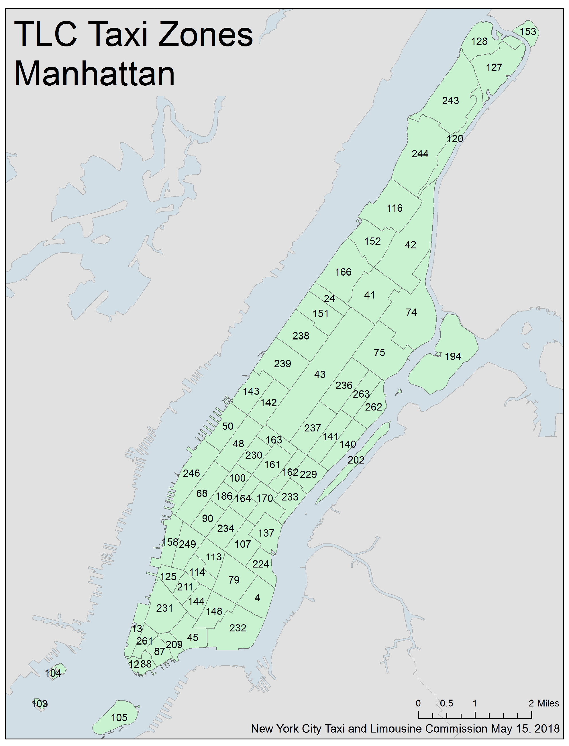
The beginning and the end of each trip are considered as one event with one location and one time of occurrence. The spatial location of these events is modeled using predefined taxi zones. Each start and end of a trip is assigned to one of these taxi zones. The New York City Taxi and Limousine Commission has divided the city into a total of 263 zones. The division of taxi zones is shown exemplarily in
Figure 2 for the borough of Manhattan. The definition of the neighborhood relations between the events is performed directly via the respective taxi zone. For this purpose, appropriate criteria are applied to the taxi zones in
Section 3.3. For the temporal reference of the events, the start and end of the taxi trips are timestamped by date and time of day.
3.2. Evaluation Methodology
The new high-frequent approach is compared with other approaches known in the literature. These include the classic Moran’s I and the extended Moran’s I index presented by Gao et al. (2019), as it has been used so far for the investigation of historical data [
7]. In addition, results from different configurations of the calculation process were also compared with each other to examine the effects of the chosen parameters.
For the evaluation of the procedure with regard to the geostatistical meaning, suitable aspects were selected, which were then examined and discussed. These aspects can be divided into two categories: (1) aspects of the evaluation that were adapted from studies on geostatistical analyses of historical data, and (2) aspects that were specifically designed for the evaluation of the approach presented in this study. In this way, comparisons with known procedures can be made and the specific capabilities and characteristics of the new approach can be considered as well.
The extended Moran’s I index presented by Gao et al. (2019) [
7] was developed to analyze mobility data. In their study, Gao et al. (2019) used data on taxi trips in Beijing to evaluate their approach [
7]. For this purpose, they conducted a comparison of the extended with the classic Moran’s I index. Separate investigations for the origin and destination of the trips were also made and compared with each other. These two comparisons have been included as aspects of the evaluation in this work. The comparison with the classic Moran’s I serves as a reference to an existing and extensively used and researched procedure. The comparison between the indices for origins and destinations provides information about mobility patterns, especially in the context of the intended dynamic view. The method presented by Liu et al. (2015) for measuring spatial autocorrelation of vectors has also been evaluated using mobility data [
24]. In this case, taxi trips in the city of Shanghai have been used. Again, the results for trip start and trip end were compared. In contrast to the study of Gao et al. (2019) [
7], the autocorrelation indicators were calculated over the course of a day for one hour at a time, rather than for the entire study period. This comparison of the values over time is also suitable for evaluating the continuous calculation of the extended Moran’s I index in this work. In this way, the dynamic view of the spatiotemporal autocorrelation can be examined. In addition to the obtained Moran’s I index, the results of the permutation tests were also compared over time. These permutation tests were represented by the arithmetic mean of all test results for the corresponding time period. Such a comparison of the determined values with the permutation tests over time is also used for the evaluation within the scope of this work.
In addition to these aspects of the evaluation, aspects addressing the continuous calculation of the extended Moran’s I index were also determined. These focus on the influence of the configuration of the analysis procedure on the results. This configuration depends on the parameter’s time interval and time span as described in
Section 2.4. For this purpose, different configurations were compared for the time interval and the time span, respectively. In addition to this, several progressions of the dynamic spatiotemporal autocorrelation over a day were compared with each other to investigate to what extent characteristic differences can be observed. In this way, further application areas for a high-frequent dynamic extended Moran’s I index can be assessed.
Beyond these comparisons of the results for the global extended Moran’s I index, the need for further result values is also considered. It is examined to what extent the additional results in the form of a map of the local extended Moran’s I indices and the Moran scatterplot, allow further statements and insights into the mobility processes. Especially with regard to the high-frequent and dynamic perspective. The selected aspects of the evaluation are summarized in
Table 2.
3.3. Assumptions and Parameters
Some assumptions need to be made and parameters must be specified in order to calculate the extended Moran’s I index. These include the spatial neighborhood relationships in the data, as well as the limits for the internal check values described in Lemmerz et al. (2023) [
6]. The parameters and assumptions defined below apply to all results presented in
Section 4.
To define the spatial neighborhood relationships, the neighborhood criterion, the order of neighborhood and the type of weighting must be specified. As the neighborhood criterion, the queen criterion was chosen [
6]. This was conducted because there was no need to distinguish the neighborhood at an edge or at a corner of the taxi zones. The mobility data collected in New York City gives reason to assume that a taxi trip can route across an edge as well as across a corner. Due to the fact that New York City is divided by two rivers and also includes several islands, some zones have direct transport links without being adjacent to each other. These transport links in the form of bridges and ferry connections were also taken as an expression of a neighborhood of two zones since they allow mutual influence on the mobility process. Only first-order neighbors were included in the spatial weights matrix. The weighting of the neighborhood relationships is carried out on the basis of binary weighting. Consequently, the relations between neighboring zones were weighted with 1, and the relations between non-neighboring zones with 0. Due to the irregular division of the taxi zones as arbitrary polygons, the weighting factors were combined in a row-standardized weights matrix. This is advantageous when the study space is irregularly subdivided. Moreover, the definition of one of the check values introduced in Lemmerz et al. (2023) is based on such a row-standardized weights matrix [
6].
In addition, threshold values for the check values explained in
Section 2.4 must also be specified. The first check value (
) must be equal to 0 according to its mathematical definition. Using a row-standardized weights matrix, the values of the global Moran’s I index equals the sum of the local indices divided by the number of localities [
6]. However, non-integer numbers are usually stored approximately in computerized data processing. For this reason, it can be expected that this check value will be non-zero but close. The data type used in the implementation of this check value stores numbers in binary format and can theoretically represent decimal numbers accurately up to 16 decimal places. However, this is linked to a large number of technical constraints. For this reason, a limit of only
was set for this check value. The second check value (
) checks to what extent the global extended Moran’s I index corresponds to the slope of the regression line in the Moran scatterplot. The slope in this regression is a legitimate estimate for Moran’s I [
29]. In the following, the global extended Moran’s I index is given with two decimal places. This gives a step size of
between two consecutive values. The limit was set to half of this step size.
4. Presentation of Results
The aspects of the evaluation outlined in
Section 3.2 were examined using the mobility data of 6 January 2018, which was a Saturday with a total of 274,468 taxi trips. Moreover, 6 January 2018 is a day with a striking pattern in terms of spatiotemporal autocorrelation and, thus, is well suited for comparison between different calculation methods and configurations. The size of the time intervals investigated in the following is selected with respect to the existing event density in the data set. In order to be able to guarantee a sufficient data basis and to be able to investigate the characteristics of a dynamic observation at the same time, time intervals in the range of several minutes were chosen. An investigation of the shortest possible time intervals in the range of a few seconds was carried out in the context of the evaluation in our previous study [
6].
In the following, the results for the different aspects of the evaluation are described and discussed. In favor of a coherent understanding of the different aspects, the aspects were divided into three groups. The first group investigates the influences of the temporal configuration parameters that were introduced to adapt the extended Moran’s I index as a streaming process. This is followed by the comparison of the results for the extended Moran’s I index with the classic Moran’s I. It allows for an assessment of the comparability of spatiotemporal autocorrelation with a well-known measure for spatial autocorrelation. In the third group of aspects, an investigation of the mobility process in the data set takes place to assess the abilities of the high-frequent dynamic autocorrelation approach. This is performed by comparing the behavior of the progression of the autocorrelation over time for the different aspects. The structure of the sections of the evaluation results and their discussion, respectively, is summarized in
Table 2. During the calculation process of the presented results, the limits for the check values defined in
Section 3.3 have been met for all values. Furthermore, the corresponding data from the previous day was also included in the calculations, so that the entire time period was considered for all the progressions presented.
4.1. Influence of the Temporal Configuration Parameters
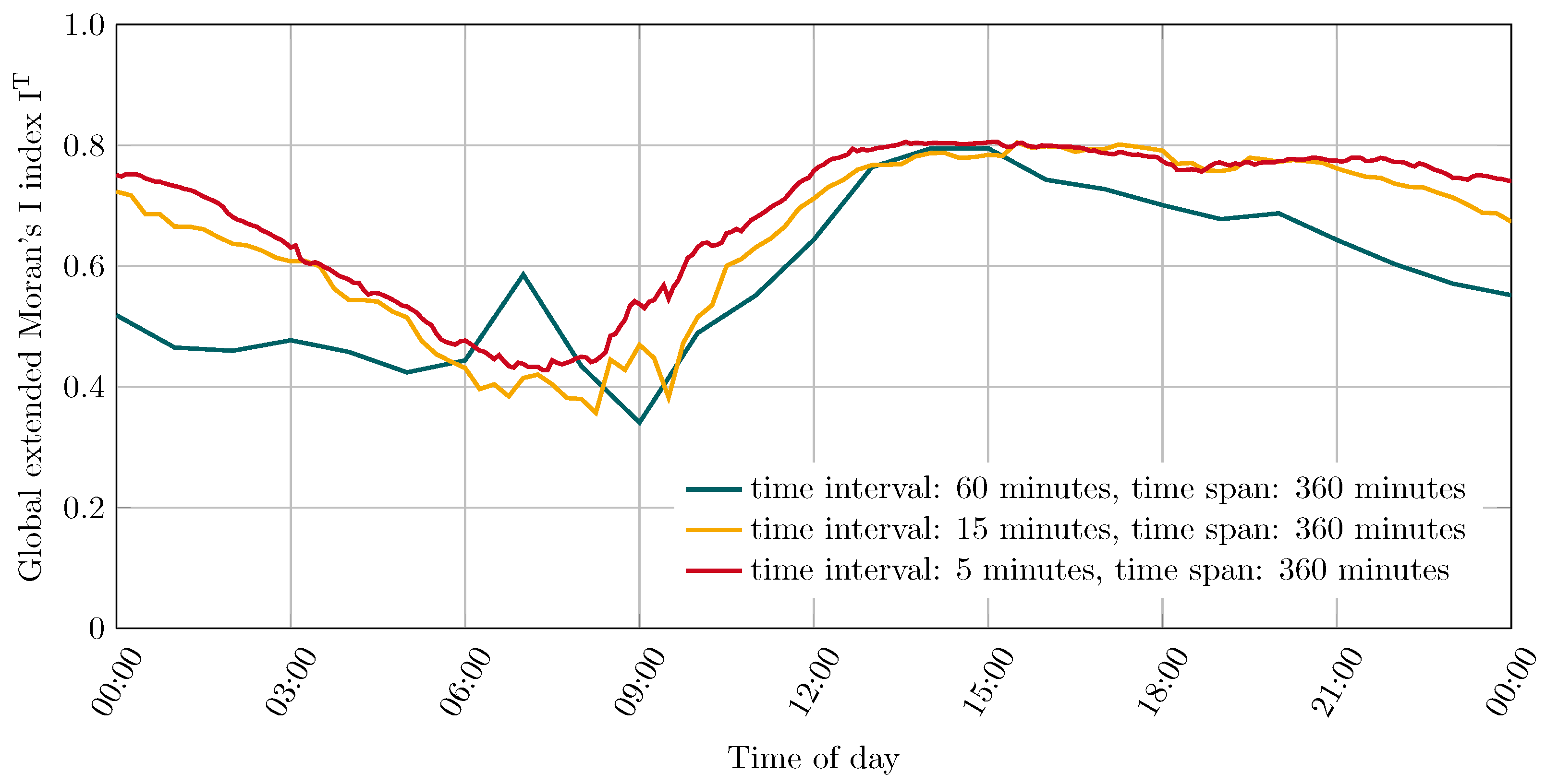
4.1.1. Comparison of Different Time Intervals
Three time intervals were compared for an assessment of the influence of the selected time interval. For this purpose, progressions of the extended Moran’s I index have been created for the intervals 5 min, 15 min, and 60 min, all with a time span of 360 min. These three progressions are shown in
Figure 3.
It can be seen that the choice of time interval has a considerable influence on the results. A division into wide intervals results in strong fluctuations, while a finer division shows a smoother progression. In the sector of the strong fluctuations (6:00 to 9:00), the progression for a time interval of 60 min stands partly in contradiction to the values of the progressions with time intervals of 5 min and 15 min. These differences can be explained by the division of the data stream into intervals. As described in
Section 2.4, the events, here starting taxi trips, are aggregated for one time interval each, and thus, an event frequency is formed for each time interval. Thus, although the total number of events that occurred does not differ, the relative growth of event frequencies over time does. These differences in the progression of event frequencies are shown in
Figure 4. This explains both, the variations in magnitude and the differences in the measured autocorrelation. The measure used to express the similarity of two time series is composed of two components: the similarity of the trend development of the time series and the size difference of the cumulated volumes of the time series. Due to the constant time span and the corresponding length of the time series, the cumulative volume is of the same size in all progressions. Consequently, the difference in the progressions arises from the differences in the trend development of the event frequencies. These differ due to the respective time interval used for their subdivision. This leads to the conclusion that the tendentially higher values for the autocorrelation are generally to be expected for a smaller time interval. Short-term differences in mobility events have less influence, since the relative proportion of influenced intervals, in relation to the length of the time series, is lower. It can be seen that shorter intervals are less influenced by increasing and decreasing event frequencies than longer time intervals. In this way, the deflection of the progression for the time interval of 60 min at 7:00 can also be explained. This division provides a sudden and highly pronounced change in the set of aggregated events between the sectors 5:00 to 6:00 and 6:00 to 7:00, which is not present in using a finer division (see
Figure 4). This produces a large disparity in the trend development, relative to the last six time intervals of 60 min each, and ultimately results in increased autocorrelation.
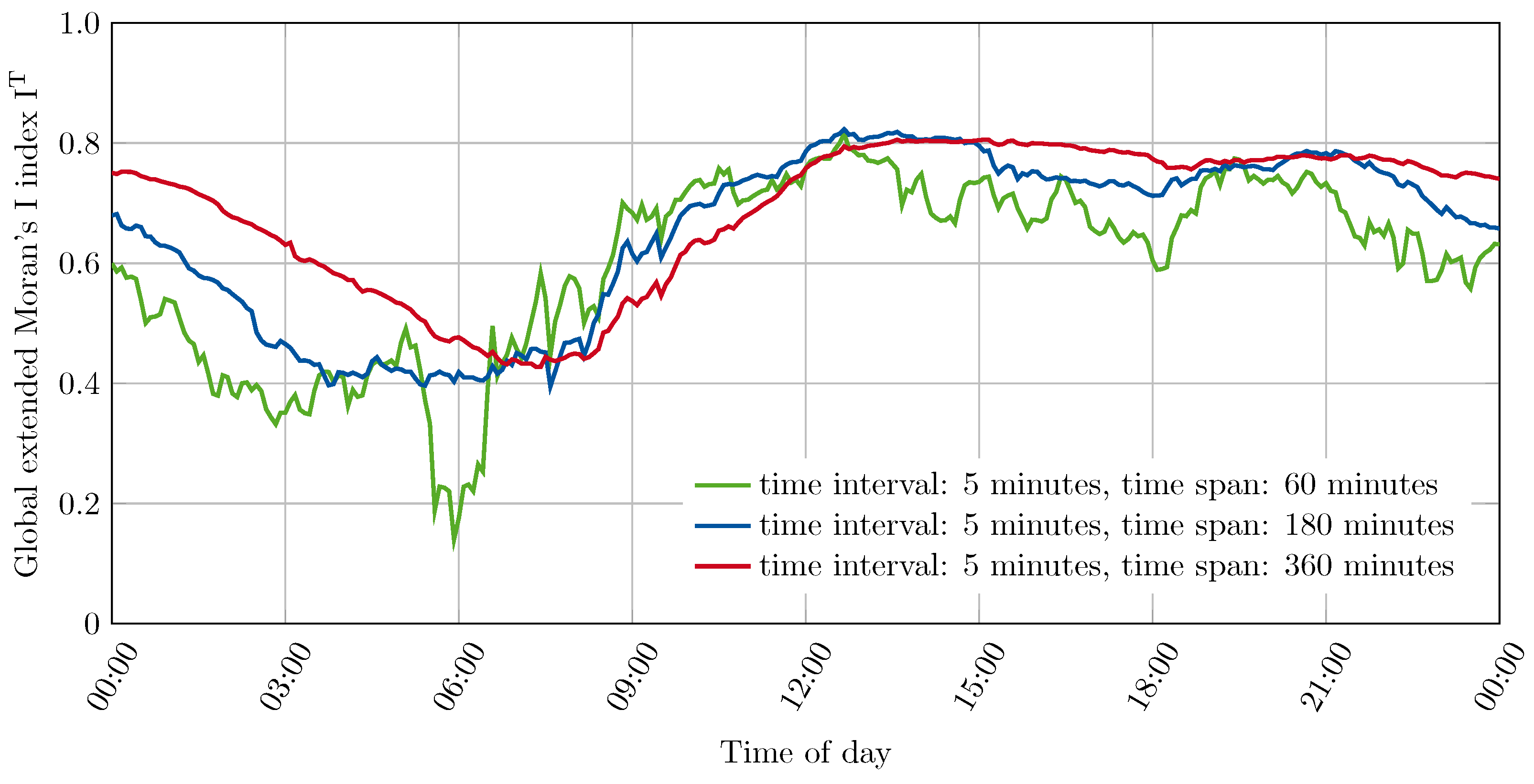
4.1.2. Comparison of Different Time Spans
Three time spans were compared to assess the impact of the chosen time span. For this purpose, progressions with a time interval of 5 min and time spans of 60 min, 180 min and 360 min have been created. These three progressions are shown in
Figure 5.
It can be seen that the choice of the time span has a significant impact on the results as well. Shorter time spans tend to result in weaker autocorrelation. On the other hand, the results show greater short-term fluctuations for shorter time spans with a generally similar progression over the day. A stronger response to changes in the mobility process can certainly be expected with a shorter observation period since individual events account for a larger share of the total data considered. Thus, a choice of shorter time spans has the effect of identifying trends earlier in the progression of the autocorrelation, since the short-term past trend is the subject of the calculation. In contrast, longer time spans result in a delayed and eased mapping of individual events. Furthermore, it can be seen that any change in the direction of the progression is more stable with a longer time span. A trend reversal of the progression for a longer time span is therefore more convincing with regard to the further development to be expected and allows a more reliable estimation of the further progression.
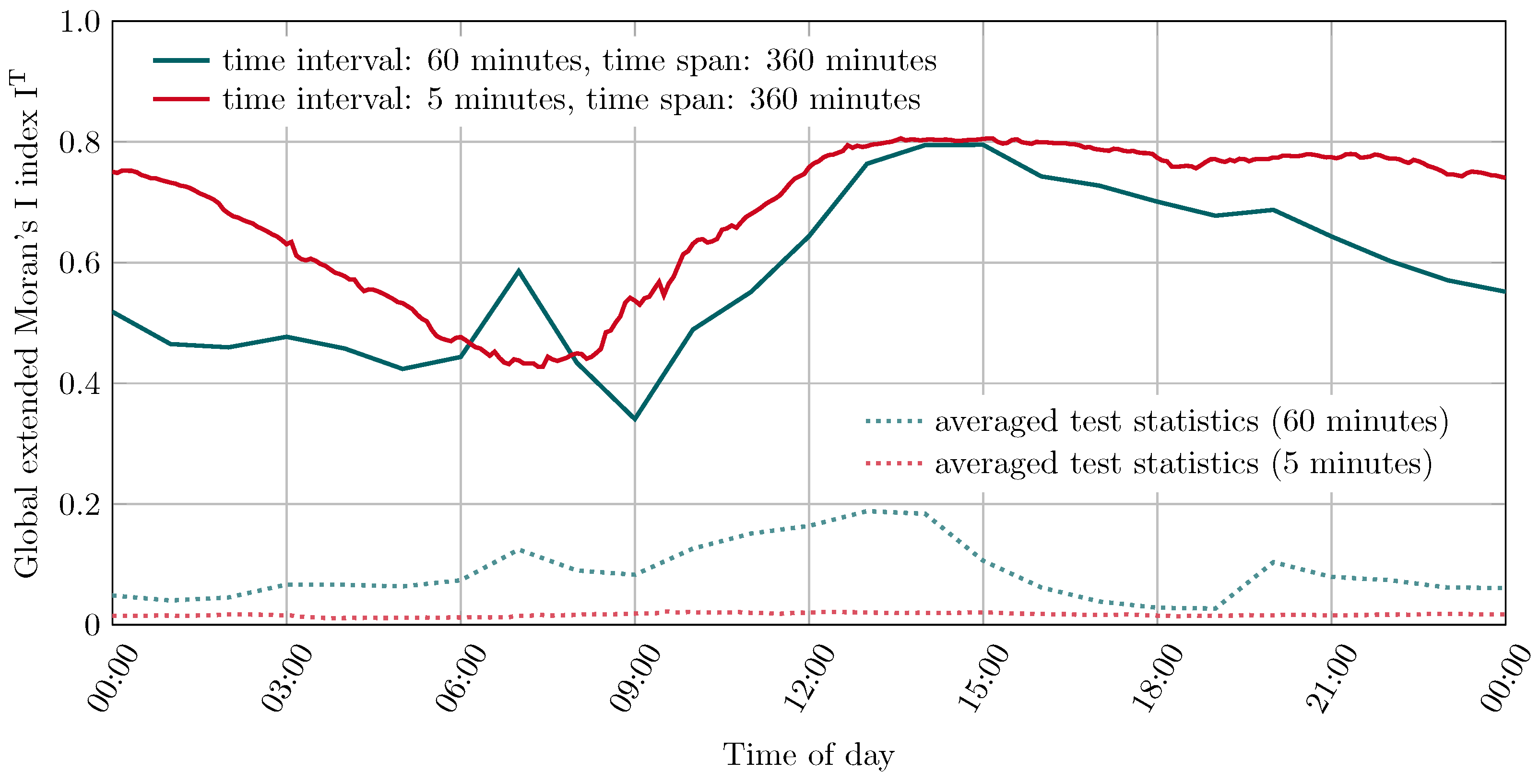
4.1.3. Comparison of the extended Morans’s I index and averaged test statistics
To compare the global extended Moran’s I index with the results of the permutation tests, two progressions with time intervals of 5 min and 60 min have been created with a time span of 360 min and 99 permutation tests performed in parallel. A pseudo-
p value of 0.01 was obtained for all time steps. The progressions are shown in
Figure 6.
It can be seen that for both time intervals, the averaged distributions from the permutation tests are considerably below the determined indices. Nevertheless, the results from the permutation tests for different time intervals show different behaviors. The averaged test statistics for the time interval of 60 min include significantly higher values and the progression is similar to the progression of the determined autocorrelation for the observed data. The averaged test statistics for the time interval of 5 min, on the other hand, are much lower and hardly reveal such a similarity in the progression. Similarities between the permutations and the actual events suggest a similarity in temporal behavior across the study space. This is because an exclusively spatial permutation of the data was performed, which otherwise should have eliminated any similarities. These similarities apparently arise only in the case of a coarse division of the time intervals. Small divisions apparently do not show these similarities in the trend development independent from the locality. Furthermore, it can be seen that especially those features can be recognized in the trend of the averaged test statistics, which distinguish the trend for the time interval of 60 min from the trend with the time interval of 5 min. This can be an indication that processes are involved that occur in the entire study area and only become noticeable in large time intervals, such as a change in the total traffic volume in the study area. Thus, similar behavior with respect to swelling and decaying event frequencies related to the selected time interval as seen in
Section 4.1.1, appears to be reflected in the permutations as well. This behavior indicates that spatiotemporal relationships in mobility events appear to be more prominent in longer time intervals due to the overall volume of traffic and thus the time of day. Accordingly, when considering short time intervals, these relationships appear to be less dependent on total traffic volume.
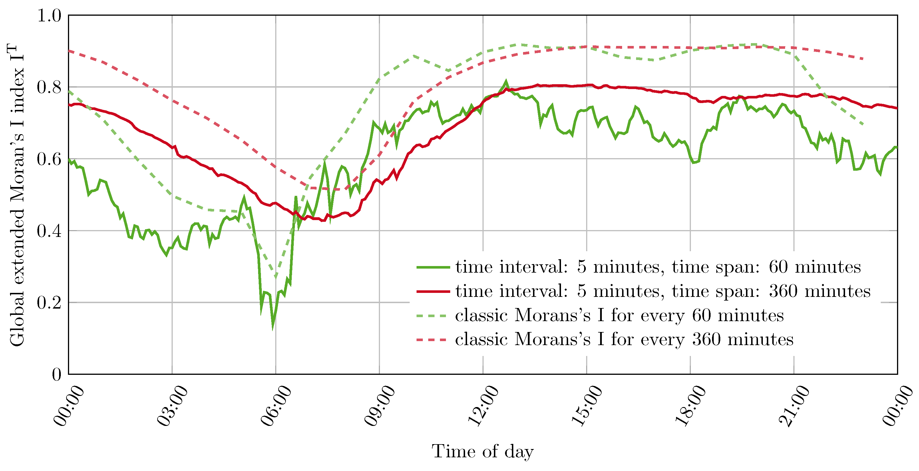
4.2. Comparison with Classic Moran’s I
Two pairs of progressions were computed to compare the high-frequent extended Moran’s I index for spatiotemporal autocorrelation with the classic Moran’s I [
16] for spatial autocorrelation. The four resulting progressions have been computed with the origin localities of the taxi trips. For the extended Moran’s I index, progressions with a time interval of 5 min were created considering data in a time span of 60 and 360 min, respectively. For comparison, the classic Moran’s I is presented for each hour, including data in each of the last 60 min and 360 min. These progressions are shown in
Figure 7.
The comparison shows that the high-frequent dynamic spatiotemporal approach provides quite comparable progressions compared to the classic Moran’s I. The development of autocorrelation over the day shows a similar progression. The autocorrelation measured by the extended Moran’s I index is usually weaker but still remains at a strong level. The observation of a stronger autocorrelation for the extended Moran’s I index compared to the classic Moran’s I, as in the study by Gao et al. (2019) [
7], cannot be confirmed here. This can be a result of a different temporal trend development occurring in the considered taxi trip data from New York City and the data from Shanghai used by Gao et al. (2019) [
7].
While the classic Moran’s I uses the accumulated volume for every locality to calculate the autocorrelation, the extended Moran’s I index by Gao et al. (2019) [
7] on the other hand, uses the accumulated volume and adjusts it by the correlation of the temporal trends in the respective localities. Considering only the calculation procedures of these two indices, a weaker autocorrelation indicates a negative correlation in the temporal trend developments of the localities. This is an insight into the mobility process, that would not have been shown by an exclusive use of spatial autocorrelation measured by the classic Moran’s I. Furthermore, it must be mentioned, that the differences may also be due to the dynamic high-frequent approach in the context of this work. An influence of the temporal configuration of the calculation procedure has already become visible in the considerations in
Section 4.1.
4.3. Investigation of the Spatiotemporal Process in the Data Set
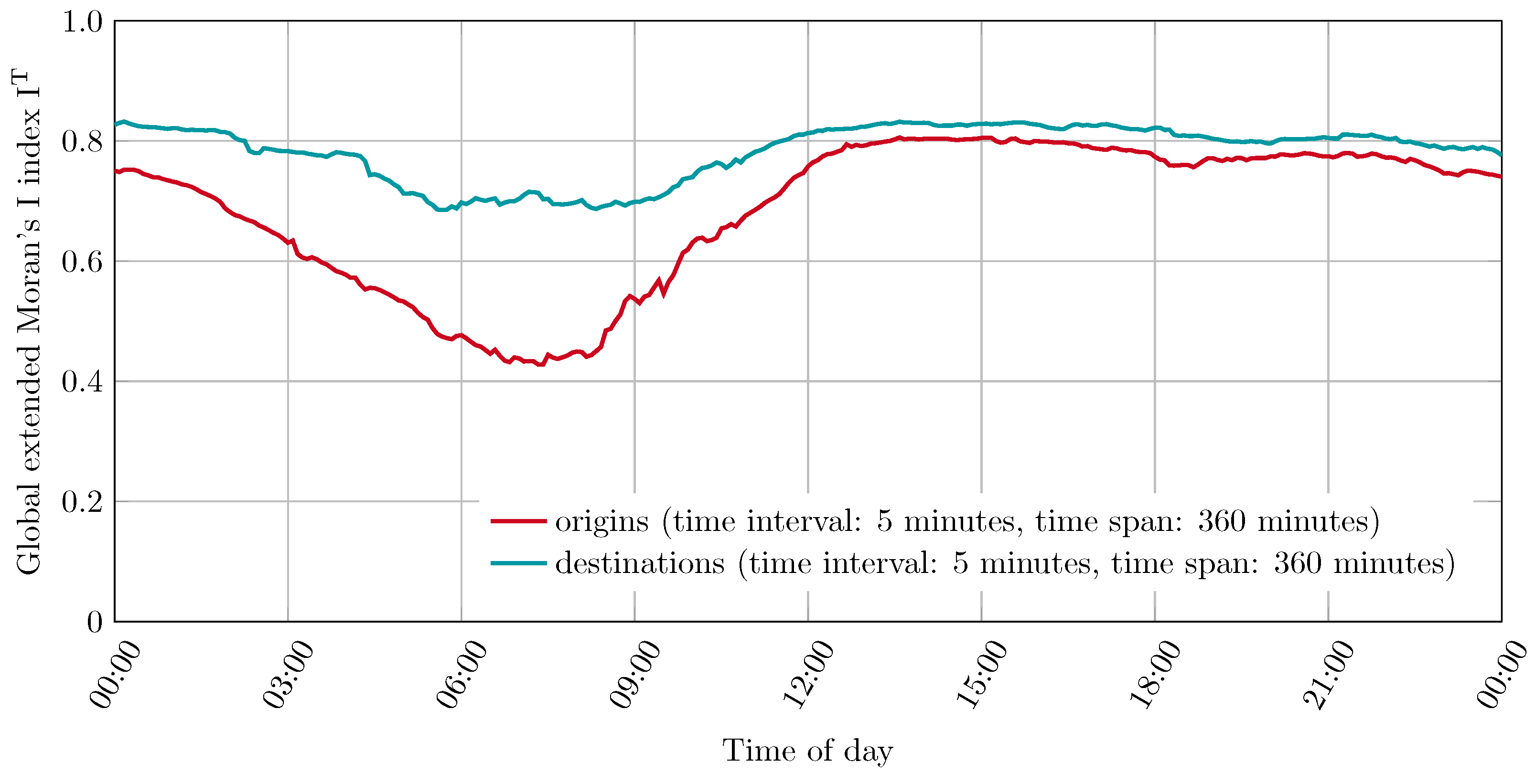
4.3.1. Comparison of Origin and Destination Localities
Differences in the autocorrelation of origin and destination localities of the taxi trips are apparent in this work, as well as in the study by Gao et al. (2019) [
7]. Progressions with a time interval of 5 min and a time span of 360 min are used to compare the two autocorrelations. These are shown in
Figure 8.
It can be seen that the observed taxi trips are generally more dispersed between 4:00 and 10:00 compared to the rest of the day. The stronger positive autocorrelation in taxi trip destinations, specifically between 5:00 and 9:00, suggests that during this period, taxi trip destinations are more concentrated than their origins. This may be related to a concentration at transportation hubs such as airports or a priority movement from a variety of neighborhoods to the city center. However, it is not possible to draw such conclusions with certainty without considering the local extended Moran’s I indices. A consideration of the local extended Moran’s I indices can be found in
Section 4.3.3.
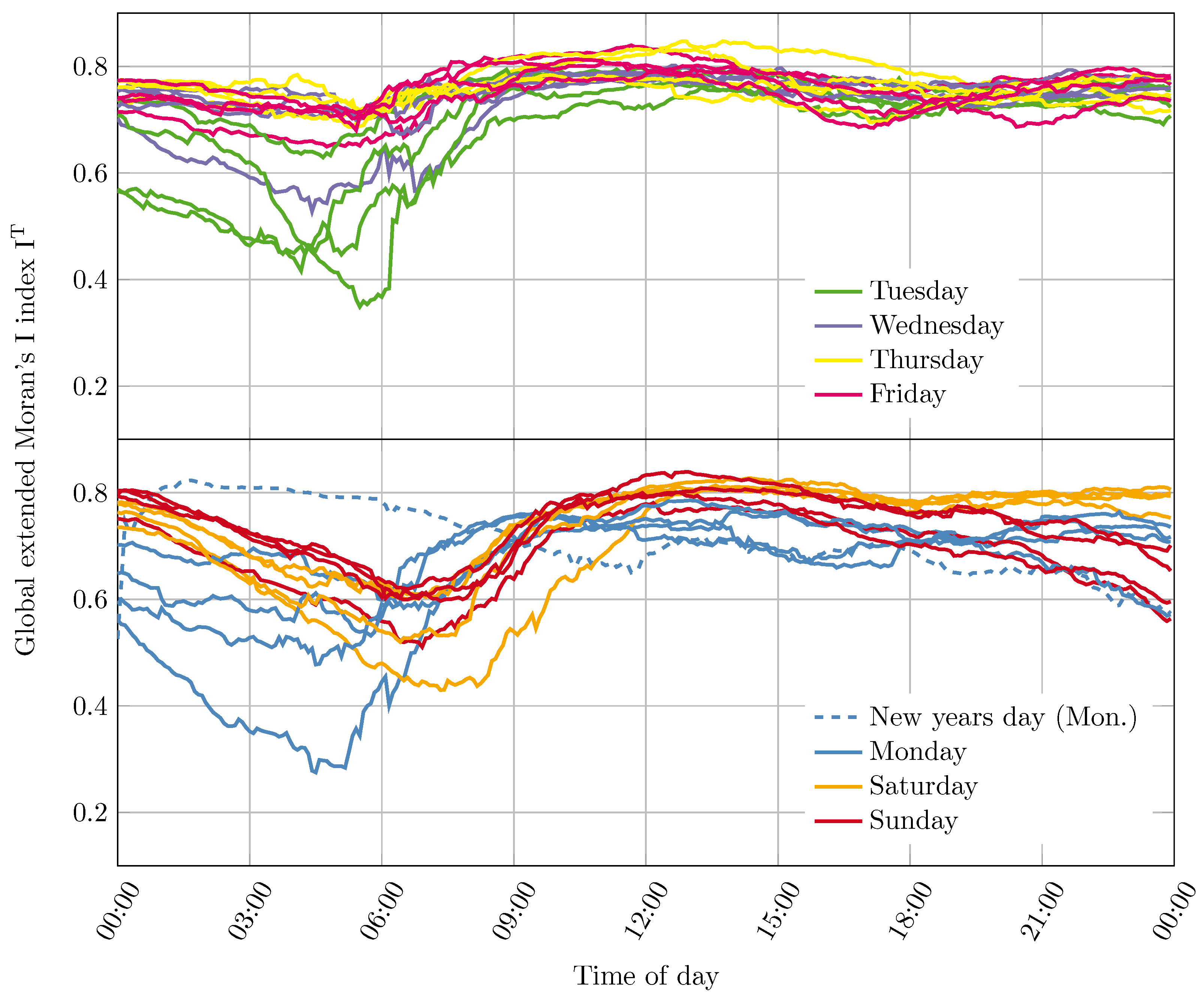
4.3.2. Comparison of Daily Progressions for Different Weekdays
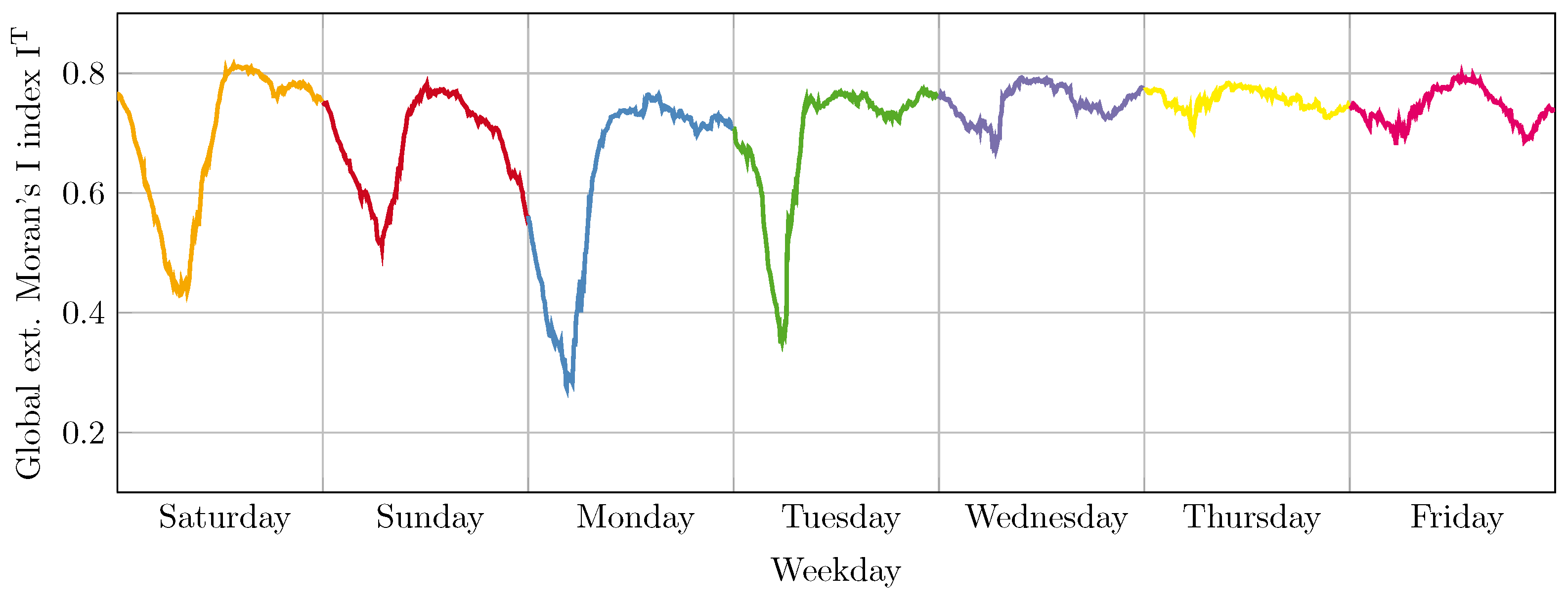
For an investigation of the behavior of the spatiotemporal autocorrelation for different weekdays, 29 progressions have been created for the global extended Moran’s I index. These progressions were created with a time interval of 5 min and a time span of 360 min in the month of January 2018 and consider the origin localities of the taxi trips.
Figure 9 shows the progressions grouped by days of the week. The first group contains the weekdays Tuesday, Wednesday, Thursday, and Friday. The second group contains the weekdays Monday, Saturday and Sunday. In addition, a progression of the spatiotemporal autocorrelation over one week, from 6–12 January 2018, is shown in
Figure 10.
A comparison of the progressions of the global extended Moran’s I index reveals that recurrent characteristics are present on certain days of the week. It is noticeable that the autocorrelation on Tuesdays often shows a depression in the period between 3:00 and 9:00, which is usually absent for the other weekdays. It is also noticeable that the majority of the progressions stay in a narrow corridor throughout the day. The weekdays Monday, Saturday and Sunday also show striking similarities between the progressions. In particular, the weekdays Saturday and Sunday are similar in their course. There is a depression in the autocorrelation in the period between 3:00 and 9:00 the usual pattern.
The difference between these two days of the week is mainly in the trend after 18:00. While the progressions on Saturdays remain at a constant high level, the values on Sundays tend to decrease. This behavior continues accordingly on the following Mondays, which is continued in clear sinks between 3:00 and 6:00. An examination of the different days of the week indicates that fluctuations in the autocorrelation occur in the period from Saturday to Tuesday, which cannot be observed from Wednesday to Friday. The progression over the week of 6–12 January 2018 in
Figure 10, impressively illustrates this different behavior within the week.
4.3.3. Consideration of Local Autocorrelation
Two observations from the previously considered comparisons were examined in more detail. For this purpose, local extended Moran’s I indices have been calculated and illustrated as colored maps and Moran scatterplots. The illustration of the local autocorrelation as a colored map allows for a better understanding of local influences on the global mobility process. The Moran scatterplot is a tool for visualizing and identifying the degree of spatial instability in a spatial association by means of Moran’s I [
29].
The first observation is the strong deviation of the global extended Moras’s I indices in the comparison between different time intervals in
Section 4.1.1 at 09:00 on 6 January 2018. The corresponding figures are grouped in
Figure 11. The second observation is the difference between the global extended Moran’s I indices in the comparison of origin and destination localities in
Section 4.3.1 at 07:10 on 6 January 2018. At this time, the largest difference between origin and destination locations occurs. This observation is shown in
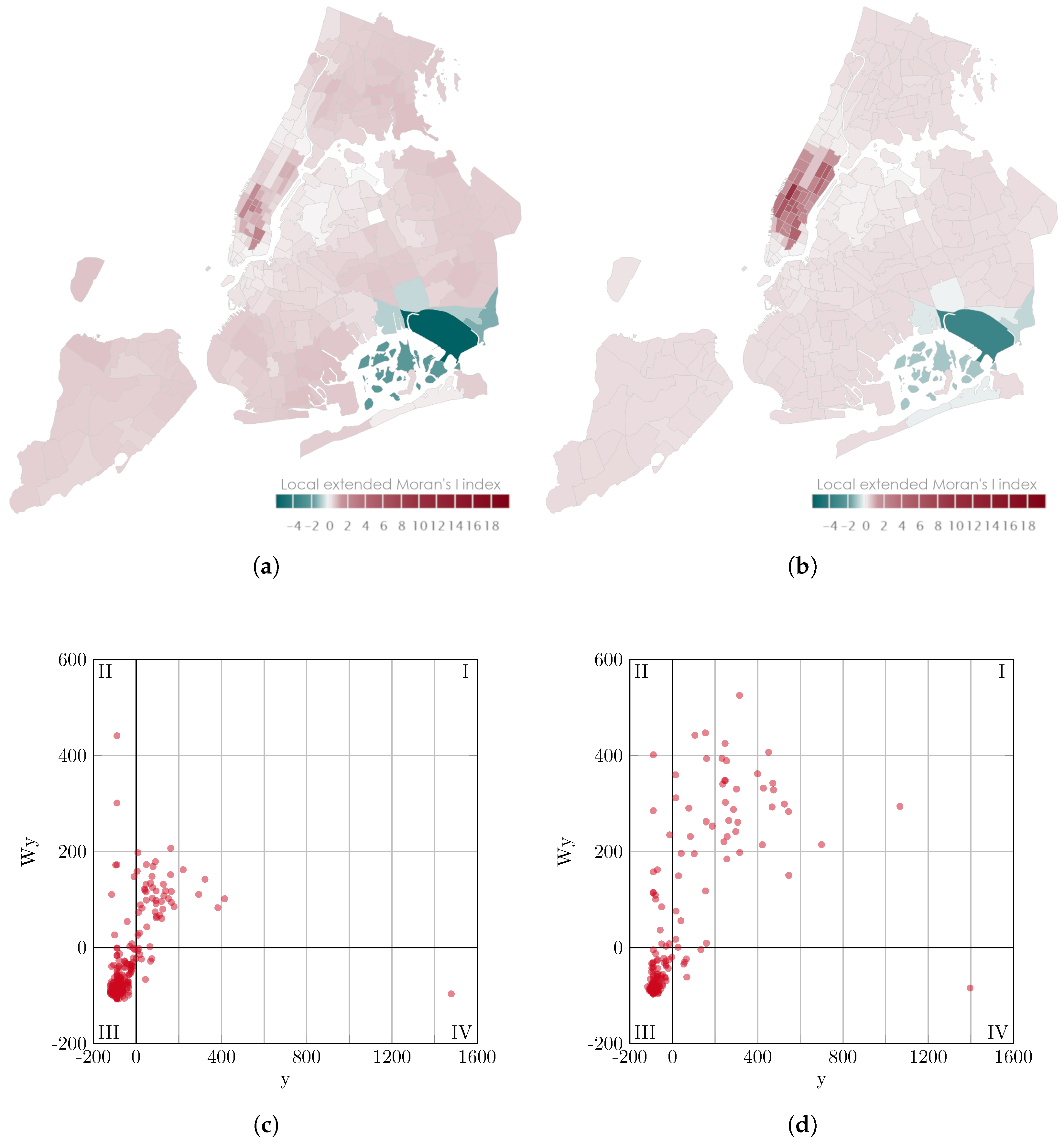
Figure 12. Shown are the map representations of the local extended Moran’s I indices in the corresponding taxi zones. Each taxi zone is colored according to the spatiotemporal autocorrelation determined for that zone. The Moran scatterplots are presented with transparent data points to reveal the accumulations of these data points.
Comparing the Moran scatterplots for the different time intervals in
Figure 11, it can be seen that both configurations show predominantly weak low-low combinations. This is particularly evident from the clusters in the third quadrants. Likewise, it can be seen that in both cases there is a strong influence from a strongly pronounced high-low combination in the fourth quadrant. The map plots reveal that this is one of the city’s airports, more precisely the John F. Kennedy Airport. The most obvious difference between the configurations can be seen in the first quadrant of the Moran scatterplot. The high-high combinations are much more pronounced at the 5 min time interval, which also reflects the stronger global extended Moran’s I index. From the map representation, it can be seen that these stronger high-high combinations primarily affect taxi zones in the Manhattan borough, the city center (see
Figure 2). Consequently, it can be concluded from the local indices and the scatterplot that the difference in the measured global spatiotemporal autocorrelation is primarily due to a stronger expression of the high-high combinations, which are restricted to a part of the urban area.
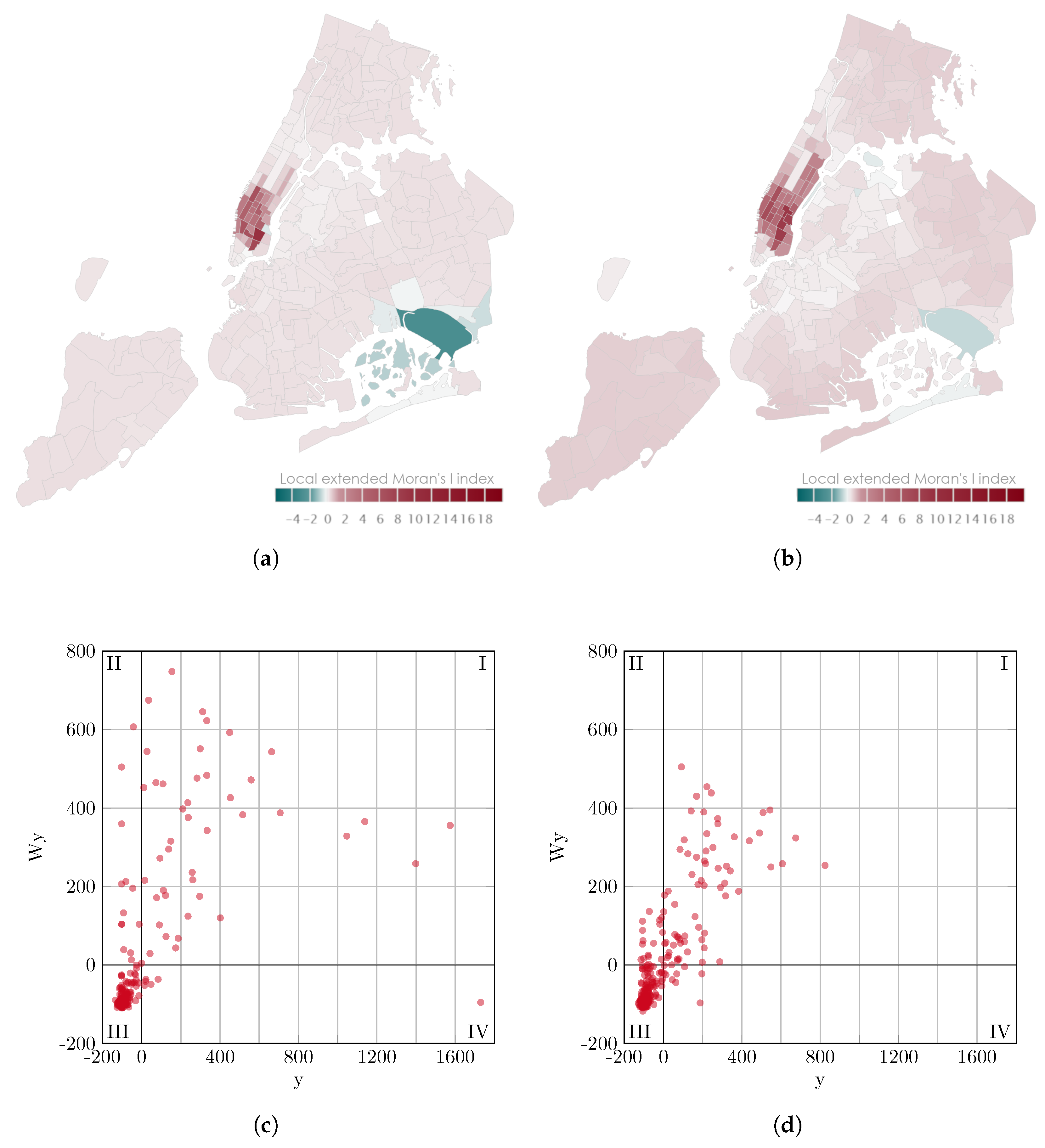
The comparison between origin and destination localities in
Figure 12 shows that both observations are mainly dominated by weak low-low combinations. It can be seen that the autocorrelation of the origin localities shows a much stronger influence of negative local indices. In particular, due to the strong high-low combination located in the fourth quadrant of the Moran scatterplot, but also by the low-high combinations located in the second quadrant, although weaker. The strongly expressed high-low combination can be identified from the map representation as the John F. Kennedy Airport. The weaker low-high combinations cluster around this zone accordingly. In contrast, a stronger expression of some high-high combinations can be seen in the third quadrants of the scatterplot for the consideration of the trip origins. The consideration of the local indices and the scatterplot suggests that the John F. Kennedy Airport has a significant impact on the differences between the global autocorrelation regarding the origin and destination localities. It can be seen that there is a local concentration of started taxi trips in this zone, while the overall global autocorrelation is weaker than for trip destinations. This can be explained by the fact that the positive local autocorrelation in the borough of Manhattan (see
Figure 2) does not show such a clear difference between started and ended taxi trips.
5. Discussion
The results of the evaluation reveal advantages and possible applications of the presented high-frequent dynamic autocorrelation, as well as limiting factors. The following section discusses the three groups of evaluation aspects as they were introduced in
Section 4 and
Table 2, respectively. First, the influences of the temporal configuration parameters are discussed. Following this, the comparison with the classic Moran’s I is discussed and the relevance of a spatiotemporal approach in the context of a high-frequent dynamic autocorrelation is highlighted. The investigation of the spatiotemporal process in the data set and the derived value of a high-frequent dynamic approach for its analysis is discussed last.
5.1. Influence of the Temporal Configuration Parameters
The investigation of the temporal configuration parameters in
Section 4.1 demonstrates the importance of the temporal configuration of the procedure. The importance of spatial configuration for a spatial autocorrelation analysis has been investigated extensively. The spatial configuration usually includes parameters such as neighborhood criteria and weighting methods. These configuration parameters are chosen just as carefully and purposefully in analyses of spatiotemporal autocorrelation. Corresponding parameters for the temporal configuration of a spatiotemporal analysis are not minor in their impact on the analysis results. Accordingly, a clear decision for or against a certain choice for the used time interval and time span cannot be made. The choice of these parameters depends on the particular goal and object of an analysis. An investigation of different configurations, as presented before, can be the basis of a reasonable configuration decision. It has been shown that shorter time intervals are less influenced by swelling and shrinking volumes of the considered events. Longer time intervals, on the other hand, are more robust against outliers or disturbances in the incoming data stream since short interruptions influence the respective interval less. For an analysis of currently occurring events, shorter intervals are also advantageous because the calculated results are updated more quickly and thus outdated results are replaced, respectively. The choice of the time span has to be balanced between a faster and stronger reaction to short-term phenomena or higher stability and reliability of the trend development. Shorter time spans allow for a quicker mapping of the processes taking place and a stronger mapping of sudden changes in the spatiotemporal autocorrelation. Longer time spans, on the other hand, are more stable and incorporate the evolution of past events over a longer period of time. Accordingly, the results are more reliable with respect to the further expected development, especially when compared with recorded traffic events from the past. Furthermore, it should be noted that none of the investigated configurations caused a negative impact on compliance with the check values defined in
Section 3.3. In summary, however, it appears that a combination of a short time interval and a long time span may be an appropriate choice for the analysis of currently occurring events. The examination of different temporal configurations in
Section 4.1 showed, that such a combination provides fast updates of the results while providing relatively stable behavior in the progression of the autocorrelation.
5.2. Comparison with Classic Moran’s I
The comparison between the classic and extended Moran’s I index, revealed consistently weaker autocorrelation when the extended Moran’s I index was applied. This is in contrast to the study of Gao et al. (2019), where stronger autocorrelations were measured [
7]. This may be due to the implementation as a continuous procedure, as well as due to differences in the data sets used, as mentioned in
Section 4.2. An influence of the chosen temporal configurations can also not be excluded. In principle, however, it can be deduced that the continuous calculation of the extended Moran’s I index provides comparable progressions to the classic Moran’s I index, while the extended Moran’s I index allows for additional consideration of the temporal trend development in the data. This is of particular interest for analyses of spatiotemporal data with high temporal resolution. The investigated mobility process in the taxi trip data does highly depend on its temporal component. Due to growing possibilities to provide such a high temporal resolution in the monitoring of such mobility processes, their temporal trend development is a considerable element next to the spatial distribution of traffic volumes alone. Beyond that, the high-frequent dynamic approach presented in this work allows for an investigation of the temporal trend development of the resulting spatiotemporal autocorrelation itself. The results show that the spatial, as well as the spatiotemporal autocorrelation is changing significantly within the scope of a day already, which further emphasizes the importance of a high-frequent dynamic autocorrelation approach.
5.3. Investigation of the Spatiotemporal Process in the Data Set
The investigation of the spatiotemporal process in the data set showed promising results regarding applications of the high-frequent dynamic autocorrelation on spatiotemporal big data. The performed comparison of different daily progressions in
Section 4.3.2 shows that the continuous and dynamic spatiotemporal autocorrelation analysis can provide additional insights to a conventional analysis based on accumulated historical data. The ability to identify characteristic progressions of autocorrelation for recurring time periods such as different days of the week, opens up the possibility to compare current events with these characteristic progressions immediately. In this way, untypical or special phenomena can be detected quickly and reliably. Such an ability to detect anomalies at an early stage can serve as a basis to develop forecasts for future trends and for proactive intervention in processes such as urban traffic. The investigation in
Section 4.3.3 shows that, especially in a continuous and dynamic analysis of the spatiotemporal autocorrelation, the local indices and also the Moran scatterplot are valuable tools to gain a deeper understanding of the measured autocorrelation. These local result values have provided further understanding of the spatial behavior of the investigated process. Furthermore, it has been shown that global spatiotemporal autocorrelation is strongly characterized by a few local extreme values. These local influencing factors are especially important for the investigation of mobility data as carried out here. In combination with the possibility to detect unusual processes by comparing the progressions of the global spatiotemporal autocorrelation with typical progressions from the past, these local values can be used to localize the origins of these anomalies. Furthermore, it is possible to assess whether only small parts or large areas of the considered area, in this case, the city of New York, are affected by such anomalies. In addition to the conclusions regarding the informative value of the procedure, a reasonable further step for examining the data set can be derived from the local result values. The significant concentration of strong local autocorrelation in the Manhattan borough argues for a separate investigation of this area. Similar to the study of Gao et al. (2019), the next step for further investigation of this data set may be to limit the study area to this central borough [
7]. Overall, it has been shown that the high-frequent dynamic spatiotemporal autocorrelation approach we presented, can reveal events in the mobility process that remain hidden from an analysis based on accumulated historical data. Due to the high-frequent dynamic approach, temporally limited unusual events can be identified and their influence on the mobility process can be investigated. The use of local autocorrelation in addition to that, allows for an identification of the spatial origin of such anomalies as well. This highlights the relevance of the presented approach as an addition to the classic Moran’s I and the original extended Moran’s I presented by Gao et al. (2019) [
7].
6. Conclusions
In this work, a high-frequent dynamic spatiotemporal autocorrelation was presented and evaluated. The goal of this study was the evaluation of a geostatistical method that provides analysis results for spatiotemporal big data in real time and an investigation of its possibilities to analyze spatiotemporal phenomena while they are still ongoing.
The conducted evaluation highlighted the importance of a high-frequent dynamic autocorrelation approach. It was shown, that an analysis of the temporal progression of the autocorrelation itself is a valuable method to investigate spatiotemporal processes, such as urban mobility. Furthermore, this approach allows for the detection of temporally limited phenomena and a deeper understanding of their occurrence and cause. It was shown that the investigation of local phenomena in the overall process is very relevant, especially in combination with such a high-frequent dynamic investigation. The consideration of the local result values for two exemplary phenomena initially detected in the global results allowed us to draw conclusions regarding their cause. In combination with the highly resolved temporal approach, underlying phenomena causing such unexpected behavior in the mobility process can be narrowed down and detected faster and way more targeted than by analyzing aggregated and historical data. Therefore, this work presents a new perspective on the temporal element of spatiotemporal autocorrelation, that is analog to the local view introduced by expanding the global perspective on the spatial element of spatiotemporal autocorrelation. The ability of this high-frequent dynamic approach to make analysis results continuously available and in real time accelerates the way we utilize spatiotemporal big data and therefore understand spatiotemporal processes in our environment.
The evaluation results also highlight the importance of the temporal configuration of the analysis procedure. The well-known spatial configurations concerning the spatial neighborhood and weighting need to be expanded by temporal criteria. In this work, the use of a time interval in combination with a time span as temporal configuration parameters was evaluated. Overall, the evaluation indicates, that a combination of a short time interval with a long time span is a good choice for analyses of temporally high resolved data.
Based on the results presented in this work, further developments are suggested. The temporal configuration parameters can be further investigated in future research to provide a deeper understanding of their impact and allow for more sophisticated choices for their respective values. Another suggestion for further investigations is the reduction in the study area to the borough of Manhattan. The results showed a concentration of high values for the local autocorrelation in this area while most of the other localities showed only mild autocorrelation. This local disparity is important for the understanding of the mobility process in New York City, but a closer look at the localities in Manhattan can probably provide further valuable insights. Furthermore, an implementation of such high-frequent dynamic analysis procedures can be used to build data services that provide geostatistical analysis results in real time as geodata streams. With such processing services, not only can the spatiotemporal data itself be made readily available, but sophisticated analysis results can be consumed in a similar way. Beyond that, spatiotemporal analysis results could be integrated into digital models of the earth and the built environment in real time.
Author Contributions
Conceptualization, Thomas Lemmerz, Stefan Herlé and Jörg Blankenbach; Methodology, Thomas Lemmerz; Validation, Thomas Lemmerz; Formal analysis, Thomas Lemmerz; Writing—original draft, Thomas Lemmerz; Writing—review and editing, Thomas Lemmerz, Stefan Herlé and Jörg Blankenbach. All authors have read and agreed to the submitted version of the manuscript.
Funding
This research received no external funding.
Conflicts of Interest
The authors declare no conflict of interest.
References
- Shi, S. Design and development of an online geoinformation service delivery of geospatial models in the United Kingdom. Environ. Earth Sci. 2015, 74, 7069–7080. [Google Scholar] [CrossRef]
- Galić, Z. Spatio-Temporal Data Streams and Big Data Paradigm. In Spatio-Temporal Data Streams; Galić, Z., Ed.; Springer: New York, NY, USA, 2016; pp. 47–69. [Google Scholar] [CrossRef]
- Evans, M.R.; Oliver, D.; Zhou, X.; Shekhar, S. Spatial Big Data: Case Studies on Volume, Velocity, and Variety; CRC Press: Boca Raton, FL, USA, 2014. [Google Scholar]
- Getis, A. A History of the Concept of Spatial Autocorrelation: A Geographer’s Perspective. Geogr. Anal. 2008, 40, 297–309. [Google Scholar] [CrossRef]
- Tiefelsdorf, M. The Saddlepoint Approximation of Moran’s I’s and Local Moran’s I i’s Reference Distributions and Their Numerical Evaluation. Geogr. Anal. 2002, 34, 187–206. [Google Scholar] [CrossRef]
- Lemmerz, T.; Herlé, S.; Blankenbach, J. Geostatistics on Real-Time Geodata Streams—An Extended Spatiotemporal Moran’s I Index with Distributed Stream Processing Technologies. ISPRS Int. J. Geo-Inf. 2023, 12, 87. [Google Scholar] [CrossRef]
- Gao, Y.; Cheng, J.; Meng, H.; Liu, Y. Measuring spatio-temporal autocorrelation in time series data of collective human mobility. Geo-Spat. Inf. Sci. 2019, 22, 166–173. [Google Scholar] [CrossRef]
- New York City Taxi and Limousine Commission. TLC Trip Record Data. 2018. New York City Taxi and Limousine Commission Website. Available online: https://www1.nyc.gov/site/tlc/about/tlc-trip-record-data.page (accessed on 23 August 2023).
- Cheng, T.; Haworth, J.; Wang, J. Spatio-temporal autocorrelation of road network data. J. Geogr. Syst. 2012, 14, 389–413. [Google Scholar] [CrossRef]
- van Zoest, V.; Osei, F.B.; Hoek, G.; Stein, A. Spatio-temporal regression kriging for modelling urban NO 2 concentrations. Int. J. Geogr. Inf. Sci. 2020, 34, 851–865. [Google Scholar] [CrossRef]
- Schneider, P.; Castell, N.; Vogt, M.; Dauge, F.R.; Lahoz, W.A.; Bartonova, A. Mapping urban air quality in near real-time using observations from low-cost sensors and model information. Environ. Int. 2017, 106, 234–247. [Google Scholar] [CrossRef]
- Lorkowski, P.; Brinkhoff, T. Environmental monitoring of continuous phenomena by sensor data streams: A system approach based on Kriging. In Proceedings of the EnviroInfo and ICT for Sustainability 2015, Copenhagen, Denmark, 7–9 September 2015; Advances in Computer Science Research. Atlantis Press: Paris, France, 2015. [Google Scholar] [CrossRef]
- Hwang, M.H.; Wang, S.; Cao, G.; Padmanabhan, A.; Zhang, Z. Spatiotemporal transformation of social media geostreams. In Proceedings of the 4th ACM SIGSPATIAL International Workshop on GeoStreaming, Orlando, FL, USA, 5 November 2013; Kazemitabar, S.J., Ed.; ACM: New York, NY, USA, 2013; pp. 12–21. [Google Scholar] [CrossRef]
- Laska, M.; Herle, S.; Klamma, R.; Blankenbach, J. A Scalable Architecture for Real-Time Stream Processing of Spatiotemporal IoT Stream Data—Performance Analysis on the Example of Map Matching. ISPRS Int. J. Geo-Inf. 2018, 7, 238. [Google Scholar] [CrossRef]
- Zhong, X.; Kealy, A.; Duckham, M. Stream Kriging: Incremental and recursive ordinary Kriging over spatiotemporal data streams. Comput. Geosci. 2016, 90, 134–143. [Google Scholar] [CrossRef]
- Moran, P.A.P. Notes on Continuous Stochastic Phenomena. Biometrika 1950, 37, 17–23. [Google Scholar] [CrossRef] [PubMed]
- Anselin, L. Local Indicators of Spatial Association-LISA. Geogr. Anal. 1995, 27, 93–115. [Google Scholar] [CrossRef]
- Geary, R.C. The Contiguity Ratio and Statistical Mapping. Inc. Stat. 1954, 5, 115. [Google Scholar] [CrossRef]
- Kibble, W.F. A Two-Variate Gamma Type Distribution. Sankhyā Indian J. Stat. 1941, 5, 137–150. [Google Scholar]
- Getis, A.; Ord, J.K. The Analysis of Spatial Association by Use of Distance Statistics. Geogr. Anal. 1992, 24, 189–206. [Google Scholar] [CrossRef]
- Ripley, B.D. The second-order analysis of stationary point processes. J. Appl. Probab. 1976, 13, 255–266. [Google Scholar] [CrossRef]
- Ord, J.K.; Getis, A. Testing for Local Spatial Autocorrelation in the Presence of Global Autocorrelation. J. Reg. Sci. 2001, 41, 411–432. [Google Scholar] [CrossRef]
- Matheron, G. Principles of geostatistics. Econ. Geol. 1963, 58, 1246–1266. [Google Scholar] [CrossRef]
- Liu, Y.; Tong, D.; Liu, X. Measuring Spatial Autocorrelation of Vectors. Geogr. Anal. 2015, 47, 300–319. [Google Scholar] [CrossRef]
- Dubé, J.; Legros, D. A spatio-temporal measure of spatial dependence: An example using real estate data*. Pap. Reg. Sci. 2013, 92, 19–30. [Google Scholar] [CrossRef]
- Lee, J.; Li, S. Extending Moran’s Index for Measuring Spatiotemporal Clustering of Geographic Events. Geogr. Anal. 2017, 49, 36–57. [Google Scholar] [CrossRef]
- Porat, I.; Shoshany, M.; Frenkel, A. Two Phase Temporal-Spatial Autocorrelation of Urban Patterns: Revealing Focal Areas of Re-Urbanization in Tel Aviv-Yafo. Appl. Spat. Anal. Policy 2012, 5, 137–155. [Google Scholar] [CrossRef]
- Douzal, A.; Nagabhushan, P. Adaptive dissimilarity index for measuring time series proximity. Adv. Data Anal. Classif. 2007, 1, 5–21. [Google Scholar] [CrossRef]
- Anselin, L.; Unwin, D.J.; Scholten, H.J.; Fischer, M.M. The Moran Scatterplot as an ESDA Tool to Assess Local Instability in Spatial Association. In Spatial Analytical Perspectives on GIS; Taylor & Francis: London, UK, 1996; pp. 111–125. [Google Scholar]
Figure 1.
Representation of time span and time interval in the data stream. Source: Lemmerz et al. [
6].
Figure 1.
Representation of time span and time interval in the data stream. Source: Lemmerz et al. [
6].
Figure 2.
Division of taxi zones in the borough of Manhattan in New York City.
Figure 2.
Division of taxi zones in the borough of Manhattan in New York City.
Figure 3.
Comparison of different time intervals in the calculation of the global extended Moran’s I index for origin localities over the course of 6 January 2018.
Figure 3.
Comparison of different time intervals in the calculation of the global extended Moran’s I index for origin localities over the course of 6 January 2018.
Figure 4.
Growth of event frequencies relative to the respective previous time interval for the entire observation area on 6 January 2018.
Figure 4.
Growth of event frequencies relative to the respective previous time interval for the entire observation area on 6 January 2018.
Figure 5.
Comparison of different time spans in the calculation of the global extended Moran’s I index for origin localities over the course of 6 January 2018.
Figure 5.
Comparison of different time spans in the calculation of the global extended Moran’s I index for origin localities over the course of 6 January 2018.
Figure 6.
Comparison of the global extended Moran’s I index with the arithmetic mean of the indices from the permutation tests for origin localities over the course of 6 January 2018.
Figure 6.
Comparison of the global extended Moran’s I index with the arithmetic mean of the indices from the permutation tests for origin localities over the course of 6 January 2018.
Figure 7.
Comparison of the global extended Moran’s I index with the global classic Moran’s I for origin localities over the course of 6 January 2018.
Figure 7.
Comparison of the global extended Moran’s I index with the global classic Moran’s I for origin localities over the course of 6 January 2018.
Figure 8.
Comparison of global extended Moran’s index for origin and destination localities over the course of 6 January 2018.
Figure 8.
Comparison of global extended Moran’s index for origin and destination localities over the course of 6 January 2018.
Figure 9.
Comparison of the global extended Moran’s I index for origin localities on different days of the week.
Figure 9.
Comparison of the global extended Moran’s I index for origin localities on different days of the week.
Figure 10.
Progression of the global extended Moran’s I index for origin localities from 6–12 January 2018.
Figure 10.
Progression of the global extended Moran’s I index for origin localities from 6–12 January 2018.
Figure 11.
Comparison of different time intervals on map plots of local extended Moran’s I indices and Moran scatterplots for 6 January 2018 at 9:00 for a time span of 360 min; in the Moran scatterplots y is the observation in deviation from the mean and Wy is the weighted average of the neighboring values. (a) time interval: 60 min, ; (b) time interval: 5 min, ; (c) time interval: 60 min, ; (d) time interval: 5 min, .
Figure 12.
Comparison of origin and destination localities on map plots of local extended Moran’s I indices and Moran scatterplots for 6 January 2018 at 7:10 for a time interval of 5 min and a time span of 360 min; in the Moran scatterplots y is the observation in deviation from the mean and Wy is the weighted average of the neighboring values. (a) origins, ; (b) destinations, ; (c) origins, ; (d) destinations, .
Table 1.
Example of a data record.
Table 1.
Example of a data record.
| Field | Value | Description |
|---|
| tpep_pickup_datetime | 2018-01-06 07:10:00.000 | Date and time at origin |
| pep_dropoff_datetime | 2018-01-06 07:17:17.000 | Date and time at destination |
| PULocationID | 234 | ID of the pick-up location |
| DOLocationID | 68 | ID of the drop-off location |
| … | | |
Table 2.
Section structure of the aspects of evaluation.
Table 2.
Section structure of the aspects of evaluation.
| Disclaimer/Publisher’s Note: The statements, opinions and data contained in all publications are solely those of the individual author(s) and contributor(s) and not of MDPI and/or the editor(s). MDPI and/or the editor(s) disclaim responsibility for any injury to people or property resulting from any ideas, methods, instructions or products referred to in the content. |
© 2023 by the authors. Licensee MDPI, Basel, Switzerland. This article is an open access article distributed under the terms and conditions of the Creative Commons Attribution (CC BY) license (https://creativecommons.org/licenses/by/4.0/).


