

Evaluation of Groundwater Vulnerability in the Upper Kelkit Valley (Northeastern Turkey) Using DRASTIC and AHP-DRASTICLu Models


Abstract
:1. Introduction
2. Materials and Methods
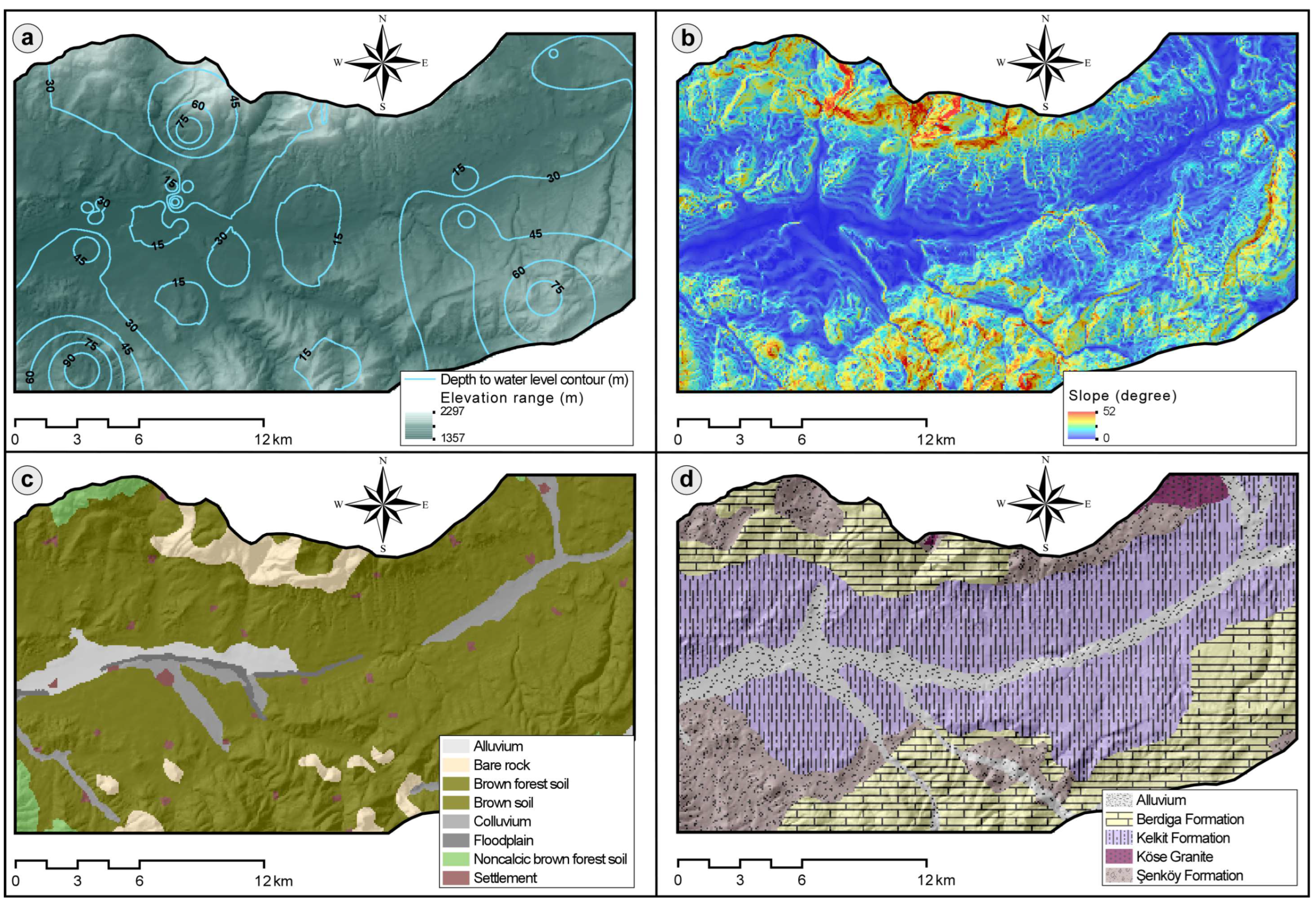
2.1. Description of the Study Area

2.2. Vulnerability Assessment Using DRASTIC and AHP-DRASTICLu Models
2.3. Weight Assignment and Normalisation of DRASTICLu Criteria Using AHP
2.4. Data Preparation and Integration into a GIS Database
2.5. Comparison and Validation of Generic DRASTIC and AHP-DRASTICLu Models
2.6. Sensitivity Analysis
3. Results and Discussion
3.1. Weighted Thematic Maps of the Criteria
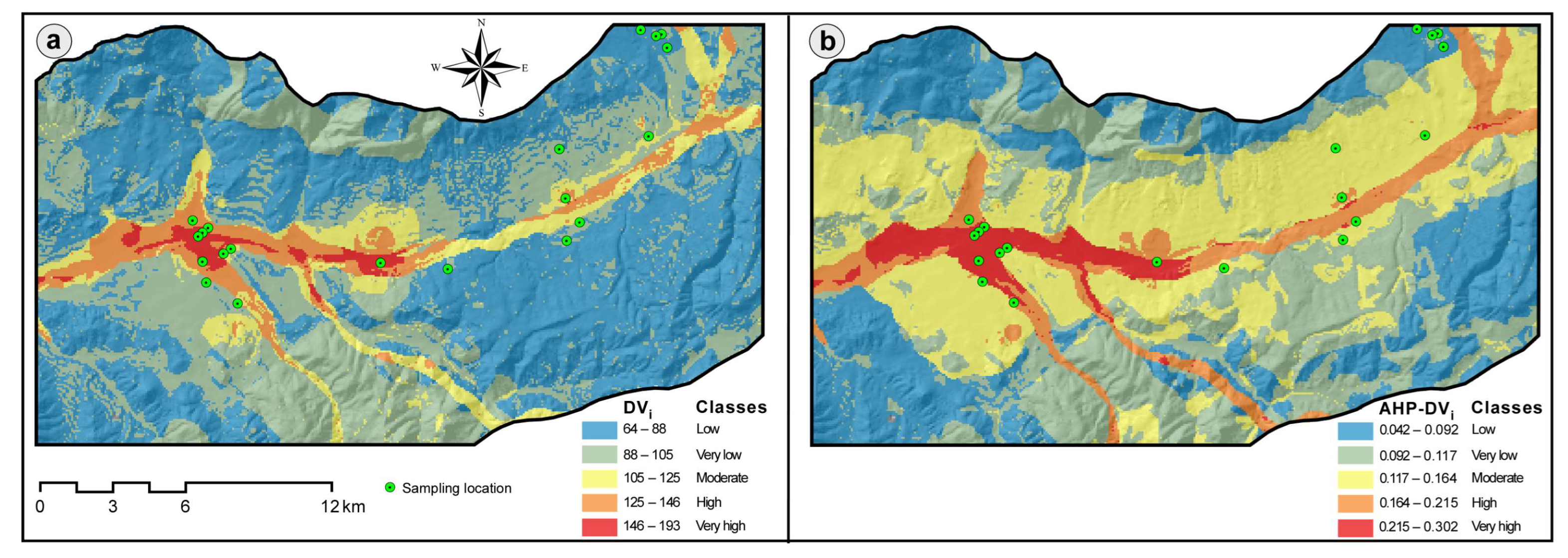
3.2. The Groundwater Vulnerability Maps of DRASTIC and AHP-DRASTICLu Models
3.3. Models’ Comparison and Validation
3.4. Single-Parameter Sensitivity Analysis
4. Conclusions
Funding
Data Availability Statement
Acknowledgments
Conflicts of Interest
References
- UNEP-United Nations Environment Programme. Adaptation Gap Report. Nairobi. 2021. Available online: https://www.unep.org/resources/adaptation-gap-report-2021 (accessed on 6 November 2022).
- Cramer, W.; Guiot, J.; Fader, M.; Garrabou, J.; Gattuso, J.P. Climate change and interconnected risks to sustainable development in the Mediterranean. Nat. Clim. Chang. 2018, 8, 972–980. [Google Scholar] [CrossRef] [Green Version]
- Şen, Ö.L. A Holistic View of Climate Change and Its Impacts in Turkey; Istanbul Policy Center, Sabancı University, Stiftung Mercator Initiative: Istanbul, Turkey, 2013. [Google Scholar]
- Reinecke, R.; Schmied, H.M.; Trautmann, T.; Andersen, L.S.; Burek, P.; Flörke, M.; Gosling, S.N.; Grillakis, M.; Hanasaki, N.; Koutroulis, A.; et al. Uncertainty of simulated groundwater recharge at different global warming levels: A global-scale multi-model ensemble study. Hydrol. Earth Syst. Sci. 2021, 25, 787–810. [Google Scholar] [CrossRef]
- WWAP. The United Nations World Water Development Report 3: Water in a Changing World, World Water Assessment Programme; UNESCO: Paris, France, 2009. [Google Scholar]
- Siebert, S.; Burke, J.; Faures, J.M.; Frenken, K.; Hoogeveen, J.; Döll, P.; Portmann, F.T. Groundwater use for irrigation—A global inventory. Hydrol. Earth Syst. Sci. 2010, 14, 1863–1880. [Google Scholar] [CrossRef] [Green Version]
- Rushton, K.R. Groundwater Hydrology: Conceptual and Computational Models; Wiley: Chichester, UK, 2003. [Google Scholar]
- Marsala, R.Z.; Capri, E.; Russo, E.; Bisagni, M.; Colla, R.; Lucini, L.; Gallo, A.; Suciu, N.A. First evaluation of pesticides occurrence in groundwater of Tidone Valley, an area with intensive viticulture. Sci. Total Environ. 2020, 736, 139730. [Google Scholar] [CrossRef]
- Bexfield, L.M.; Kenneth, B.; Lindsey, B.D.; Toccalino, P.L.; Nowell, L.H. Pesticides and pesticide degradates in groundwater used for public supply across the United States: Occurrence and human-health context. Environ. Sci. Technol. 2021, 55, 362–372. [Google Scholar] [CrossRef] [PubMed]
- Güler, C.; Kurt, M.A.; Alpaslan, M.; Akbulut Camuzcuoğlu, C. Assessment of the impact of anthropogenic activities on the groundwater hydrology and chemistry in Tarsus coastal plain Mersin SE Turkey using fuzzy clustering multivariate statistics and GIS techniques. J. Hydrol. 2012, 414, 435–451. [Google Scholar] [CrossRef]
- United Nations Committee on Economic Social and Cultural Rights. General Comment No. 15 (2002). In The Right to Water; E/C.12/2002/11; United Nations Social and Economic Council: Geneva, Switzerland, 2003; 18p. [Google Scholar]
- UN DESA. The Sustainable Development Goals Report 2022. New York, USA. 2022. Available online: https://unstats.un.org/sdgs/report/2022/ (accessed on 21 February 2023).
- EU Water Framework Directive: Directive 2000/60/EC of the European Parliament and of the Council Establishing a Framework for the Community Action in the Field of Water Policy. Available online: https://eur-lex.europa.eu/eli/dir/2000/60/oj (accessed on 6 November 2022).
- United Nations. Johannesburg Plan of Implementation of the World Summit on Sustainable Development; United Nations: Geneva, Switzerland, 2002; 72p. [Google Scholar]
- United Nations. World Water Development Report 2: Water, a Shared Responsibility; UNESCO: Paris, France, 2006; 601p. [Google Scholar]
- World Water Council. Final Report of the 4th World Water Forum; National Water Commission of Mexico: Mexico City, Mexico, 2006; 262p. [Google Scholar]
- Margat, J. Vulnérabilité des Nappes d’eau Souterraine à la Pollution: Bases de la Cartographie; BRGM Publication No. 68 SGL 198 HYD; BRGM (Bureau de Recherches Géologiques et Miniéres): Orléans, France, 1968. [Google Scholar]
- Evans, B.M.; Myers, W.L. A GIS-based approach to evaluating regional groundwater pollution potential with DRASTIC. J. Soil Water Conserv. 1990, 45, 242–245. [Google Scholar]
- Van Stempvoort, D.; Ewert, L.; Wassenaar, L. Aquifer vulnerability index: GIS-compatible method for groundwater vulnerability mapping. Can. Water Resour. J. 1993, 18, 25–37. [Google Scholar] [CrossRef] [Green Version]
- Hiscock, K.M.; Lovett, A.A.; Brainard, J.S.; Parfitt, J.P. Groundwater vulnerability assessment: Two case studies using GIS methodology. Q. J. Eng. Geol. Hydrogeol. 1995, 28, 179–194. [Google Scholar] [CrossRef]
- Civita, M.; De-Regibus, C. Sperimentazione di alcune metodologie per la valutazione della vulnerabilita’ degli aquiferi. In Quaderni di GeologiaApplicata, Pitagora Edition; Pitagora Editrice: Bologna, Italy, 1995. [Google Scholar]
- Foster, S.S.D. Fundamental concepts in aquifer vulnerability, pollution risk and protection strategy. In Vulnerability of Soil and Groundwater to Pollutants; Duijvenbooden, W., Waegeningh, H.G., Eds.; Committee on Hydrological Research: The Hague, The Netherlands, 1987; pp. 69–86. [Google Scholar]
- Aller, L.; Lehr, J.; Petty, R. DRASTIC: A Standardized System to Evaluate Groundwater Pollution Potential Using Hydrogeologic Settings; Bennett, T., Ed.; National Water Well Association: Worthington, OH, USA; Bennett and Williams, Inc.: Columbus, OH, USA, 1987; 43229p. [Google Scholar]
- Doerfliger, N.; Jeannin, P.Y.; Zwahlen, F. Water vulnerability assessment in karst environments: A new method of defining protection areas using a multi-attribute approach and GIS tools (EPIK method). Environ. Geol. 1999, 39, 165–176. [Google Scholar] [CrossRef] [Green Version]
- Goldscheider, N.; Klute, M.; Sturm, S.; Hötzl, H. The PI method—A GIS-based approach to mapping groundwater vulnerability with special consideration of karst aquifers. Z. Für Angew. 2000, 46, 157–166. [Google Scholar]
- Vias, J.M.; Andrea, B.; Perles, M.J.; Carrasco, F.; Vadillo, I.; Jimenez, P. Proposed method for groundwater vulnerability mapping in carbonate (Karstic) aquifers: The COP Method. Hydrogeol. J. 2006, 14, 912–925. [Google Scholar] [CrossRef]
- Babiker, I.S.; Mohamed, M.A.A.; Hiyama, T.; Kato, K. A GIS-based DRASTIC model for assessing aquifer vulnerability in Kakamigahara Heights, Gifu Prefecture, central Japan. Sci. Total Environ. 2005, 345, 127–140. [Google Scholar] [CrossRef] [PubMed]
- Rahman, A.A. GIS based DRASTIC model for assessing groundwater vulnerability in shallow aquifer in Aligarh, India. Appl. Geogr. 2008, 28, 32–53. [Google Scholar] [CrossRef]
- Güler, C.; Kurt, M.A.; Korkut, R.N. Assessment of groundwater vulnerability to nonpoint source pollution in a Mediterranean Coastal Zone (Mersin, Turkey) under conflicting Landuse practices. Ocean Coast. Manag. 2013, 71, 141–152. [Google Scholar] [CrossRef]
- Pacheco, F.A.L.; Sanches Fernandes, L.F. The multivariate statistical structure of DRASTIC model. J. Hydrol. 2013, 476, 442–459. [Google Scholar] [CrossRef]
- Wei, A.; Bi, P.; Guo, J.; Lu, S.; Li, D. Modified DRASTIC model for groundwater vulnerability to nitrate contamination in the Dagujia river basin, China. Water Supply 2021, 21, 1793–1805. [Google Scholar] [CrossRef]
- Maqsoom, A.; Aslam, B.; Khalil, U.; Ghorbanzadeh, O.; Ashraf, H.; Faisal Tufail, R.; Farooq, D.; Blaschke, T. A GIS-based DRASTIC model and an adjusted DRASTIC model (DRASTICA) for groundwater susceptibility assessment along the China–Pakistan Economic Corridor (CPEC) Route. ISPRS Int. J. Geo Inf. 2020, 9, 332. [Google Scholar] [CrossRef]
- Mkumbo, N.J.; Mussa, K.R.; Mariki, E.E.; Mjemah, I.C. The Use of the DRASTIC-LU/LC model for assessing groundwater vulnerability to nitrate contamination in Morogoro Municipality, Tanzania. Earth 2022, 3, 1161–1184. [Google Scholar] [CrossRef]
- Ckakraborty, S.; Paul, P.K.; Sikdar, P.K. Assessing aquifer vulnerability to arsenic pollution using DRASTIC and GIS of North Bengal Plain: A case study of English Bazar Block, Malda District, West Bengal, India. J. Spat. Hydrol. 2007, 7, 101–121. [Google Scholar]
- Saidi, S.; Bouri, S.; Ben Dhia, H. Sensitivity analysis in groundwater vulnerability assessment based on GIS in the Mahdia-Ksour Essaf aquifer, Tunisia: A validation study. Hydrol. Sci. J. 2011, 56, 288–304. [Google Scholar] [CrossRef]
- Huan, H.; Wang, J.; Teng, Y. Assessment and validation of groundwater vulnerability to nitrate based on a modified DRASTIC model: A case study in Jilin City of northeast China. Sci. Total Environ. 2012, 440, 14–23. [Google Scholar] [CrossRef] [PubMed]
- Tilahun, K.; Merkel, B.J. Estimation of groundwater recharge using a GIS-based distributed water balance model in Dire Dawa, Ethiopia. Hydrogeol. J. 2009, 17, 1443–1457. [Google Scholar] [CrossRef]
- Kumar, A.; Pramod Krishna, A. Groundwater vulnerability and contamination risk assessment using GIS-based modified DRASTIC-LU model in hard rock aquifer system in India. Geocarto Int. 2020, 35, 1149–1178. [Google Scholar] [CrossRef]
- Neshat, A.; Pradhan, B.; Pirasteh, S.; Shafri, H.Z.M. Estimating groundwater vulnerability to pollution using a modified DRASTIC model in the Kerman agricultural area, Iran. Environ. Earth Sci. 2014, 71, 3119–3131. [Google Scholar] [CrossRef]
- Saranya, T.; Saravanan, S.; Jennifer, J.J.; Singh, L. Assessment of groundwater vulnerability in highly industrialized Noyyal basin using AHP-DRASTIC and Geographic Information System. In Disaster Resilience and Sustainability; Pal, I., Djalante, I., Shav, R., Shrestha, S., Eds.; Elsevier: Amsterdam, The Netherlands, 2007; pp. 151–170. [Google Scholar] [CrossRef]
- Bera, A.; Mukhopadhyay, B.P.; Das, S. Groundwater vulnerability and contamination risk mapping of semi-arid Totko river basin, India using GIS-based DRASTIC model and AHP techniques. Chemosphere 2022, 307, 135831. [Google Scholar] [CrossRef]
- Saranya, T.; Saravanan, S. Evolution of a hybrid approach for groundwater vulnerability assessment using hierarchical fuzzy-DRASTIC models in the Cuddalore Region. India. Environ. Earth Sci. 2021, 80, 1–25. [Google Scholar] [CrossRef]
- Maretto, L.; Faccio, M.; Battini, D. A Multi-Criteria Decision-Making model based on fuzzy logic and AHP for the selection of digital technologies. IFAC-PapersOnLine 2022, 55, 319–324. [Google Scholar] [CrossRef]
- Saranya, T.; Saravanan, S. Assessment of groundwater vulnerability using analytical hierarchy process and evidential belief function with DRASTIC parameters, Cuddalore, India. Int. J. Environ. Sci. Technol. 2023, 20, 1837–1856. [Google Scholar] [CrossRef]
- Pacheco, F.; Pires, L.; Santos, R.; Sanches Fernandes, L. Factor weighting in DRASTIC modeling. Sci. Total Environ. 2015, 505, 474–486. [Google Scholar] [CrossRef]
- Murgai, R.; Ali, M.; Byerlee, D. Productivity growth and sustainability in postgreen revolution agriculture: The case for the Indian and Pakistan Punjabs. World Bank Res. Obser. 2001, 16, 199–218. [Google Scholar] [CrossRef]
- Gelberg, K.H.; Church, L.; Casey, G.; London, M.; Roerig, D.S.; Boyd, J.; Hill, M. Nitrate levels in drinking water in rural New York State. Environ. Res. 1999, 80, 34–40. [Google Scholar] [CrossRef]
- TSMS (Turkish State Meteorological Service) MEVBİS. Available online: https://mevbis.mgm.gov.tr/mevbis/ui/index.html (accessed on 12 November 2022).
- TUIK (Turkish Statistical Institute) Address Based Population Statistics of Turkey 2021. Available online: https://data.tuik.gov.tr/Bulten/Index?p=Adrese-Dayali-Nufus-Kayit-Sistemi-Sonuclari-2021-45500 (accessed on 12 December 2022).
- GDRS (General Directorate of Rural Services). Soil Characteristics Map of Scale 1/25.000; GDRS: Ankara, Turkey, 2001. [Google Scholar]
- Güven, İ.H. Doğu Karadeniz Bölgesi’nin 1/25.000 Ölçekli Jeolojisi ve Komplikasyonu; MTA: Ankara, Turkey, 1993. [Google Scholar]
- EEA (European Environment Agency). Copernicus Land Service—Pan-European Component: CORINE Land Cover 2000. European Environment Agency: Copenhagen. Available online: https://land.copernicus.eu/pan-european/corine-land-cover/clc-2000?tab=download (accessed on 2 December 2022).
- EEA (European Environment Agency). Copernicus Land Service—Pan-European Component: CORINE Land Cover 2006. European Environment Agency: Copenhagen. Available online: https://land.copernicus.eu/pan-european/corine-land-cover/clc-2006?tab=download (accessed on 2 December 2022).
- EEA (European Environment Agency). Copernicus Land Service—Pan-European Component: CORINE Land Cover 2012. European Environment Agency: Copenhagen. Available online: https://land.copernicus.eu/pan-european/corine-land-cover/clc-2012?tab=download (accessed on 2 December 2022).
- EEA (European Environment Agency). Copernicus Land Service—Pan-European Component: CORINE Land Cover 2018. European Environment Agency: Copenhagen. Available online: https://land.copernicus.eu/pan-european/corine-land-cover/clc2018?tab=download (accessed on 2 December 2022).
- Topuz, G.; Altherr, R.; Wolfgang, S.; Schwarz, W.H.; Zack, T.; Hasanözbek, A.; Mathias, B.; Satır, M.; Şen, C. Carboniferous high-potassium I-type granitoid magmatism in the Eastern Pontides: The Gümüşhane pluton (NE Turkey). Lithos 2010, 116, 92–110. [Google Scholar] [CrossRef]
- Dokuz, A. A salb detachment and delemanition model for the generation of Carboniferous high potassium I-type magmatisim in the Easrtern Pontides: The Köse composite Pluton. Gondwana Res. 2011, 19, 926–944. [Google Scholar] [CrossRef]
- Yazıcı, N. Kelkit ve Köse (Gümüşhane) Ilçe Merkezi Içme Sularının Hidrojeokimyasal Özellikleri Ile Yan Kayaçlarla Olan Ilişkilerinin Incelenmesi. Master’s Thesis, Gümüşhane University Institute of Science, Gümüşhane, Turkey, 2019. [Google Scholar]
- Robinson, A.G.; Banks, C.J.; Rutherford, M.M.; Hirst, J.P.P. Stratigraphic and structural development of the Eastern Pontides, Turkey. J. Geol. Soc. Lond. 1995, 152, 861–872. [Google Scholar] [CrossRef]
- Şen, C. Jurassic volcanism in the Eastern Pontides: Is it rift related or subduction related? Turk. J. Earth Sci. 2007, 16, 523–539. Available online: https://journals.tubitak.gov.tr/earth/vol16/iss4/6 (accessed on 16 November 2022).
- Kandemir, R.; Yılmaz, C. Lithostratigraphy, facies and deposition environment of the Lower Jurassic Ammonitico Rosso Type Sediments (ARTS) in the Gumushane Area, NE Turkey: Implications for the opening of the Northern branch of the Neo-Tethys Ocean. J. Asian Earth Sci. 2009, 34, 586–598. [Google Scholar] [CrossRef]
- Taslı, K. Gümüşhane-Bayburt Yörelerindeki Üst Jura-Alt Kretase Yaşlı Karbonat Istiflerinin Stratigrafisi ve Mikropaleontolojik Incelemesi. Ph.D. Thesis, Karadeniz Technical University Graduate Institute of Natural and Applied Sciences, Trabzon, Turkey, 1990. [Google Scholar]
- Yılmaz, C. Kelkit (Gümüşhane) yöresinin stratigrafisi. Jeoloji Mühendisliği 1992, 40, 50–62. Available online: https://www.jmo.org.tr/resimler/ekler/2a6845a557bef70_ek.pdf?dergi=JEOLOJ%DD%20M%DCHEND%DDSL%DD%D0%DD%20DERG%DDS%DD (accessed on 16 November 2022).
- Saydam Eker, Ç.; Sipahi, F.; Kaygusuz, A. Trace and rare earth elements as indicators of provenance and depositional environments of Lias Cherts in Gumushane NE Turkey. Geochemistry 2012, 72, 167–177. [Google Scholar] [CrossRef]
- Arslan, M.; Aliyazıcıoğlu, I. Geochemical and Petrological Characteristics of the Kale (Gümüshane) volcanic rocks: Implications for the Eocene evolution of Eastern Pontide arc volcanism, Northeast Turkey. Int. Geol. Rev. 2001, 43, 595–610. [Google Scholar] [CrossRef]
- GDSHW (General Directorate of State Hydraulic Works)—Akım Gözlem Yıllıkları. Available online: https://www.dsi.gov.tr/Sayfa/Detay/744# (accessed on 14 December 2022).
- Soyaslan, I.I. Assessment of groundwater vulnerability using modified DRASTIC-Analytical Hierarchy Process model in Bucak Basin, Turkey. Arab. J. Geosci. 2020, 13, 1127. [Google Scholar] [CrossRef]
- Saaty, T.L. The Analytic Hierarchy Process: Planning, Priority Setting, Resources Allocation; McGraw: New York, NY, USA, 1980. [Google Scholar]
- Karahan, M. Bulak (Kelkit, Gümüşhane) Göleti Aks Yeri ve Göl Alanındaki Kayaçların Geçirimlilik Özelliklerinin Araştırılması. Master’s Thesis, Karadeniz Technical University Graduate Institute of Natural and Applied Sciences, Trabzon, Turkey, 2015. [Google Scholar]
- Piscopo, G. Groundwater Vulnerability Map Explanatory Notes, Macquarie Catchment. NSW Department of Land and Water Conservation. Sydney, Australia, 2001. Available online: https://www.dpie.nsw.gov.au/__data/assets/pdf_file/0010/151768/Macquarie-map-notes.pdf (accessed on 1 December 2022).
- Aydınalp, C.; Arslan, Y. Batı karadeniz havzasındaki büyük toprak gruplarının FAO/UNESCO (1990), Fitzpatrick (1988) ve toprak taksonomisi (USDA soil taxonomy, 1994) sistemlerine göre sınıflandırılması. ANADOLU Ege Tarımsal Araştırma Enstitüsü Derg. 2003, 13, 188–200. Available online: https://dergipark.org.tr/tr/pub/anadolu/issue/1774/21842 (accessed on 17 November 2022).
- Tümsavaş, Z.; Aksoy, E. Kahverengi orman büyük toprak grubu topraklarının verimlilik durumlarının belirlenmesi. J. Agric. Fac. Bursa Uludag Univ. 2009, 23, 93–104. Available online: https://dergipark.org.tr/tr/download/article-file/154090 (accessed on 17 November 2022).
- Zeybek, İ. Turhal ovası ve yakın çevresi toprakları. Türk Coğrafya Dergisi 2003, 41, 41–61. Available online: https://dergipark.org.tr/tr/download/article-file/198552 (accessed on 17 November 2022).
- Singh, A.; Srivastav, S.K.; Kumar, S.; Chakrapani, G.J. A modified-DRASTIC model (DRASTICA) for assessment of groundwater vulnerability to pollution in an urbanized environment in Lucknow, India. Environ. Earth Sci. 2015, 74, 5475–5490. [Google Scholar] [CrossRef]
- Bedient, P.B.; Rifai, H.S.; Newell, C.J. Ground Water Contamination: Transport and Remediation; Prentice Hall: Upper Saddle River, NJ, USA, 1999. [Google Scholar]
- Spearman Rank Correlation Coefficient. In The Concise Encyclopedia of Statistics; Springer: New York, NY, USA, 2008; 502p. [CrossRef]
- Napolitano, P.; Fabbri, A.G. Single-parameter sensitivity analysis for aquifer vulnerability assessment using DRASTIC and SINTACS. In HydroGIS 96: Application of Geographical Information Systems in Hydrology and Water Resources Management, Proceedings of the Vienna Conference, Vienna, Austria, 16–19 April 1996; IAHS Pub.: Wallingford, UK, 1996; Volume 235, pp. 559–566. [Google Scholar]
- Boulding, J.R. Practical Handbook of Soil, Vadose Zone, and Ground-Water Contamination: Assessment, Prevention, and Remediation; CRC Press, Inc.: Boca Raton, FL, USA, 1995. [Google Scholar]
- Saidi, S.; Bouri, S.; Dhia, H.B. Groundwater management based on GIS techniques, chemical indicators and vulnerability to seawater intrusion modelling: Application to the Mahdia-Ksour Essaf aquifer, Tunisia. Environ. Earth Sci. 2013, 70, 1551–1568. [Google Scholar] [CrossRef]
- Zhang, Y.; Qin, H.; An, G.; Huang, T. Vulnerability assessment of farmland groundwater pollution around traditional industrial parks based on the improved DRASTIC Model—A case study in Shifang City, Sichuan Province, China. Int. J. Environ. Res. Public Health 2022, 19, 7600. [Google Scholar] [CrossRef] [PubMed]
- Abera, K.A.; Gebreyohannes, T.; Abrha, B.; Hagos, M.; Berhane, G.; Hussien, A.; Belay, A.S.; Van Camp, M.; Walraevens, K. Vulnerability mapping of groundwater resources of Mekelle City and surroundings, Tigray Region, Ethiopia. Water 2022, 14, 2577. [Google Scholar] [CrossRef]
- Jasrotia, A.S.; Singh, R. Groundwater pollution vulnerability using the DRASTIC model in a GIS environment, Devak-Rui Watersheds, India. J. Environ. Hydrol. 2005, 13, 11. Available online: http://www.hydroweb.com/jeh/jeh2005/jasrotia.pdf (accessed on 22 November 2022).
- Brady, N.C.; Weil, R.R. The Nature and Properties of Soils; Prentice Hall: Englewood Cliffs, NJ, USA, 2002. [Google Scholar]
- Chakraborty, B.; Roy, S.; Bera, A.; Adhikary, P.P.; Bera, B.; Sengupta, D.; Shit, P.K. Groundwater vulnerability assessment using GIS-based DRASTIC model in the upper catchment of Dwarakeshwar river basin, West Bengal, India. Environ. Earth Sci. 2022, 81, 1–15. [Google Scholar] [CrossRef]
- Ersoy, A.F.; Gültekin, F. DRASTIC-based methodology for assessing groundwater vulnerability in the Gümüşhacıköy and Merzifon Basin (Amasya, Turkey). Earth Sci. Res. J. 2013, 17, 33–40. [Google Scholar]
- Arafa, N.A.; Salem, Z.E.-S.; Ghorab, M.A.; Soliman, S.A.; Abdeldayem, A.L.; Moustafa, Y.M.; Ghazala, H.H. Evaluation of groundwater sensitivity to pollution using GIS-based modified DRASTIC-LU model for sustainable development in the Nile Delta Region. Sustainability 2022, 14, 14699. [Google Scholar] [CrossRef]
- Secunda, S.; Collin, M.L.; Melloul, A.J. Groundwater vulnerability assessment using a composite model combining DRASTIC with extensive agricultural land use in Israel’s Sharon region. J. Environ. Manag. 1998, 54, 39–57. [Google Scholar] [CrossRef]
- Huang, Y.; Zuo, R.; Li, J.; Wu, J.; Zhai, Y.; Teng, Y. The spatial and temporal variability of groundwater vulnerability and human health risk in the Limin District, Harbin, China. Water 2018, 10, 686. [Google Scholar] [CrossRef] [Green Version]
- Sener, E.; Davraz, A. Assessment of groundwater vulnerability based on a modified DRASTIC model, GIS and an analytic hierarchy process (AHP) method: The case of Egirdir Lake basin (Isparta, Turkey). Hydrogeol. J. 2013, 21, 701–714. [Google Scholar] [CrossRef]
- Hem, J.D. Study and Interpretation of the Chemical Characteristics of Natural Water; Water Supply Paper; U.S. Geological Survey: Washington, DC, USA, 1985; p. 2254.
- Sharma, M.K.; Kumar, M. Sulphate contamination in groundwater and its remediation: An overview. Environ. Monit. Assess. 2020, 192, 74. [Google Scholar] [CrossRef]
- Liu, J.; Han, G. Tracing riverine sulfate source in an agricultural watershed: Constraints from stable isotopes. Environ. Pollut. 2021, 228, 117740. [Google Scholar] [CrossRef]
- Wang, H.; Zhang, Q. Research advances in identifying sulfate contamination sources of water environment by using stable isotopes. Int. J. Environ. Res. Public Health 2019, 16, 1914. [Google Scholar] [CrossRef] [Green Version]
- Roy, A.; Keesari, T.; Mohokar, H.; Sinha, U.K.; Bitra, S. Assessment of groundwater quality in hard rock aquifer of central Telangana state for drinking and agriculture purposes. Appl. Water Sci. 2018, 8, 124. [Google Scholar] [CrossRef] [Green Version]
- Javed, T.; Sarwar, T.; Ullah, I.; Ahmad, S.; Rashid, S. Evaluation of groundwater quality in district Karak Khyber Pakhtunkhwa, Pakistan. Water Sci. 2019, 33, 1–9. [Google Scholar] [CrossRef] [Green Version]
- Lerner, D.N. Estimating Urban Loads of Nitrogen to Groundwater. Water Environ. J. 2003, 17, 239–244. [Google Scholar] [CrossRef]
- Kurt, M.A.; Güler, C.; Alpaslan, M.; Akbulut, C. Determination of nitrate and nitrite origins in the soils and ground waters of the area between Mersin-Tarsus (Turkey) using geographic information systems. Carpathian J. Earth Environ. Sci. 2012, 7, 181–188. [Google Scholar]
- Karadavut, İ.S.; Saydam, A.C.; Kalıpçı, E.; Karadavut, S.; Özdemir, C. A research for water pollution of Melendiz stream in terms of sustainability of ecological balance. Carpathian J. Earth Environ. Sci. 2011, 6, 65–80. [Google Scholar]
- Prasanth, S.S.; Magesh, N.; Jitheshlal, K.; Chandrasekar, N.; Gangadhar, K. Evaluation of groundwater quality and its suitability for drinking and agricultural use in the coastal stretch of Alappuzha District, Kerala, India. Appl. Water Sci. 2012, 2, 165–175. [Google Scholar] [CrossRef] [Green Version]
- Saravanan, S.; Pitchaikani, S.; Thambiraja, M.; Sathiyamurthi, S.; Sivakumar, V.; Velusamy, S.; Shanmugamoorthy, M. Comparative assessment of groundwater vulnerability using GIS-based DRASTIC and DRASTIC-AHP for Thoothukudi District, Tamil Nadu India. Environ. Monit. Assess. 2023, 195, 57. [Google Scholar] [CrossRef]
- Awais, M.; Aslam, B.; Maqsoom, A.; Khalil, U.; Ullah, F.; Azam, S.; Imran, M. Assessing Nitrate Contamination Risks in Groundwater: A Machine Learning Approach. Appl. Sci. 2021, 11, 10034. [Google Scholar] [CrossRef]
- Jahromi, M.N.; Gomeh, Z.; Busico, G.; Barzegar, R.; Samany, N.N.; Aalami, M.T.; Tedesco, D.; Mastrocicco, M.; Kazakis, N. Developing a SINTACS-based method to map groundwater multi-pollutant vulnerability using evolutionary algorithms. Environ. Sci. Pollut. Res. 2021, 28, 7854–7869. [Google Scholar] [CrossRef] [PubMed]
- Dhaoui, O.; Antunes, I.; Agoubi, B.; Kharroubi, A. Integration of water contamination indicators and vulnerability indices on groundwater management in Menzel Habib area, south-eastern Tunisia. Environ. Res. 2022, 205, 112491. [Google Scholar] [CrossRef]
- Hasan, M.; Islam, M.A.; Aziz Hasan, M.; Alam, M.J.; Peas, M.H. Groundwater vulnerability assessment in Savar upazila of Dhaka district, Bangladesh—A GIS-based DRASTIC modeling. Groundw. Sustain. Dev. 2019, 9, 100220. [Google Scholar] [CrossRef]
- Salek, M.; Levison, J.; Parker, B.; Gharabaghi, B. CAD-DRASTIC: Chloride application density combined with DRASTIC for assessing groundwater vulnerability to road salt application. Hydrogeol. J. 2018, 26, 2379–2393. [Google Scholar] [CrossRef]
- Moratalla, Á.; Gómez-Alday, J.J.; Sanz, D.; Castaño, S.; De Las Heras, J. Evaluation of a GIS-based integrated vulnerability risk assessment for the Mancha Oriental System (SE Spain). Water Resour. Manag. 2011, 25, 3677–3697. [Google Scholar] [CrossRef]
- Sakala, E.; Fourie, F.; Gomo, M.; Coetzee, H. GIS-based groundwater vulnerability modelling: A case study of the Witbank, Ermelo and Highveld Coalfields in South Africa. J. Afr. Earth Sci. 2018, 137, 46–60. [Google Scholar] [CrossRef]
- Jamrah, A.; Al-Futaisi, A.; Rajmohan, N.; Al-Yaroubi, S. Assessment of groundwater vulnerability in the coastal region of Oman using DRASTIC index method in GIS environment. Environ. Monit. Assess. 2008, 147, 125–138. [Google Scholar] [CrossRef] [PubMed]
- Haidu, I.; Nistor, M. Groundwater vulnerability assessment in the Grand Est region, France. Quat. Int. 2020, 547, 86–100. [Google Scholar] [CrossRef]


| Characteristics | Unit | Value | Characteristics | Unit | Value |
|---|---|---|---|---|---|
| The study area (total) | km2 | 445 | Soil type | ||
| Meteorology | Brown soil | % area | 77.12 | ||
| Precipitation (total mean) | mm/year | 300 | Brown forest soil | % area | 5.84 |
| Temperature (mean) | °C | 6.5 | Bare rock | % area | 5.25 |
| Slope range | Colluvium | % area | 4.69 | ||
| 0°–2° | % area | 6.28 | Noncalcic brown forest soil | % area | 2.16 |
| 2°–6° | % area | 18.61 | Alluvium | % area | 3.03 |
| 6°–12° | % area | 21.08 | Settlement | % area | 0.96 |
| 12°–18° | % area | 15.02 | Floodplain | % area | 0.94 |
| >18° | % area | 39.01 | Geology | ||
| Elevation range (a.m.s.l.) | Kelkit Formation | % area | 44.01 | ||
| 1357–1500 m | % area | 25.03 | Berdiga Formation | % area | 28.36 |
| 1500–1750 m | % area | 54.72 | Şenköy Formation | % area | 15.30 |
| 1750–2000 | % area | 17.62 | Alluvium | % area | 11.18 |
| 2000–2297 m | % area | 2.64 | Köse Granite | % area | 1.15 |
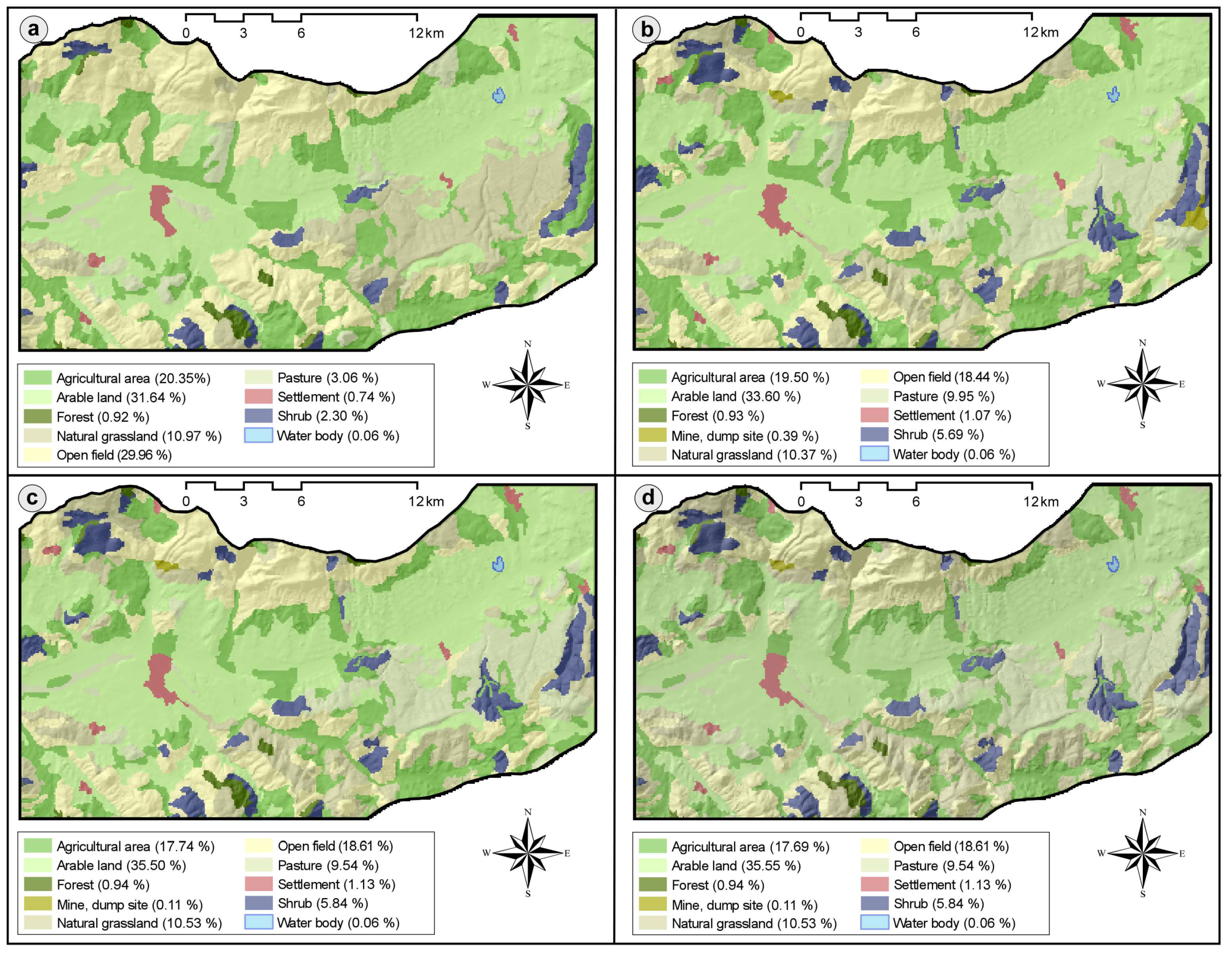
| Land Use/Land Classes | 2000 | 2006 | 2012 | 2018 * |
|---|---|---|---|---|
| Agricultural area | 20.35 | 19.50 | 17.74 | 17.69 |
| Arable land | 31.64 | 33.60 | 35.55 | 35.55 |
| Forest | 0.92 | 0.93 | 0.94 | 0.94 |
| Natural grassland | 10.97 | 10.37 | 10.53 | 10.53 |
| Open field | 29.96 | 18.44 | 18.61 | 18.61 |
| Pasture | 3.06 | 9.95 | 9.54 | 9.54 |
| Settlement | 0.74 | 1.07 | 1.13 | 1.13 |
| Shrub | 2.30 | 5.69 | 5.84 | 5.84 |
| Water body | 0.06 | 0.06 | 0.06 | 0.06 |
| Mine and dump site | - | 0.39 | 0.11 | 0.11 |
| Main Criteria | (D) | (R) | (A) | (S) | (T) | (I) | (C) | (Lu) | AHP-DRASTICLu wi | DRASTIC wi |
|---|---|---|---|---|---|---|---|---|---|---|
| (D) Depth to water table | 1 | 0.248 | 5 | |||||||
| (R) Net recharge | 1/2 | 1 | 0.143 | 4 | ||||||
| (A) Aquifer media | 1/3 | 1/2 | 1 | 0.081 | 3 | |||||
| (S) Soil media | 1/7 | 1/3 | 1/2 | 1 | 0.047 | 2 | ||||
| (T) Topography | 1/9 | 1/6 | 1/4 | 1/3 | 1 | 0.024 | 1 | |||
| (I) Impact of vadose zone | 1 | 2 | 4 | 3 | 7 | 1 | 0.237 | 5 | ||
| (C) Hydraulic conductivity | 1/3 | 1/3 | 1/2 | 2 | 3 | 1/4 | 1 | 0.065 | 3 | |
| (Lu) Land use classes | 1/2 | 1 | 3 | 5 | 6 | 1/2 | 2 | 1 | 0.154 |
| Subcriteria | (1) | (2) | (3) | (4) | (5) | (6) | (7) | (8) | (9) | (10) | AHP-DRASTICLu | DRASTIC | ||||
|---|---|---|---|---|---|---|---|---|---|---|---|---|---|---|---|---|
| ri | wi | ri × wi | ri | wi | ri × wi | |||||||||||
| Depth to water table (m) | 0.248 | 5 | ||||||||||||||
| (1) 0–1.52 | 1 | 0.352 | 0.0876 | 10 | 50 | |||||||||||
| (2) 1.52–4.57 | 1/2 | 1 | 0.231 | 0.0573 | 9 | 45 | ||||||||||
| (3) 4.57–9.14 | 1/3 | 1/2 | 1 | 0.157 | 0.0389 | 7 | 35 | |||||||||
| (4) 9.14–15.24 | 1/4 | 1/3 | 1/2 | 1 | 0.112 | 0.0278 | 5 | 25 | ||||||||
| (5) 15.24–22.86 | 1/5 | 1/4 | 1/3 | 1/2 | 1 | 0.075 | 0.0186 | 3 | 15 | |||||||
| (6) 22.86–30.48 | 1/7 | 1/5 | 1/4 | 1/4 | 1/2 | 1 | 0.051 | 0.0126 | 2 | 10 | ||||||
| (7) 30.48< | 1/9 | 1/7 | 1/7 | 1/6 | 1/6 | 1/5 | 1 | 0.022 | 0.0055 | 1 | 5 | |||||
| Net recharge | 0.143 | 4 | ||||||||||||||
| (1) Very low | 1 | 0.041 | 0.0059 | 1 | 4 | |||||||||||
| (2) Low | 2 | 1 | 0.056 | 0.0081 | 3 | 12 | ||||||||||
| (3) Moderate | 3 | 5 | 1 | 0.149 | 0.0213 | 5 | 20 | |||||||||
| (4) High | 7 | 6 | 2 | 1 | 0.276 | 0.0395 | 8 | 32 | ||||||||
| (5) Very high | 9 | 7 | 5 | 2 | 1 | 0.478 | 0.0684 | 10 | 40 | |||||||
| Aquifer media | 0.081 | 3 | ||||||||||||||
| (1) Alluvium | 1 | 0.433 | 0.0351 | 8 | 24 | |||||||||||
| (2) Massive limestone | 1/2 | 1 | 0.255 | 0.0208 | 7 | 21 | ||||||||||
| (3) Badded sandstone, limestone, and shale | 1/3 | 1/2 | 1 | 0.174 | 0.0141 | 6 | 18 | |||||||||
| (4) Igneous | 1/7 | 1/5 | 1/4 | 1 | 0.046 | 0.0037 | 4 | 12 | ||||||||
| (5) Weathered metamorphic/igneous | 1/5 | 1/3 | 1/3 | 3 | 1 | 0.091 | 0.0074 | 5 | 15 | |||||||
| Soil media | 0.047 | 2 | ||||||||||||||
| (1) Alluvium | 1 | 0.145 | 0.0068 | 9 | 18 | |||||||||||
| (2) Brown soil | 1/5 | 1 | 0.047 | 0.0022 | 5 | 10 | ||||||||||
| (3) Bare rock | 3 | 5 | 1 | 0.263 | 0.0124 | 10 | 20 | |||||||||
| (4) Floodplain | 2 | 4 | 1/2 | 1 | 0.172 | 0.0082 | 9 | 18 | ||||||||
| (4) Colluvium | 1/3 | 3 | 1/3 | 1/4 | 1 | 0.079 | 0.0037 | 6 | 12 | |||||||
| (5) Brown forest soil | 1/5 | 1/2 | 1/5 | 1/5 | 1/3 | 1 | 0.035 | 0.0016 | 3 | 6 | ||||||
| (6) Noncalcic brown forest soil | 1/5 | 1/2 | 1/5 | 1/5 | 1/3 | 1 | 1 | 0.037 | 0.0017 | 3 | 6 | |||||
| (7) Settlement | 2 | 5 | 1/2 | 3 | 5 | 4 | 3 | 1 | 0.221 | 0.0104 | 10 | 20 | ||||
| Topography (slope %) | 0.024 | 1 | ||||||||||||||
| (1) 0–2 | 1 | 0.424 | 0.0102 | 10 | 10 | |||||||||||
| (2) 2–6 | 1/2 | 1 | 0.287 | 0.0069 | 9 | 9 | ||||||||||
| (3) 6–12 | 1/3 | 1/2 | 1 | 0.162 | 0.0039 | 5 | 5 | |||||||||
| (4) 12–18 | 1/5 | 1/5 | 1/2 | 1 | 0.086 | 0.0022 | 3 | 3 | ||||||||
| (5) 18< | 1/5 | 1/6 | 1/5 | 1/3 | 1 | 0.042 | 0.0010 | 1 | 1 | |||||||
| Impact of vadose zone | 0.237 | 5 | ||||||||||||||
| (1) Alluvium | 1 | 0.431 | 0.1022 | 8 | 40 | |||||||||||
| (2) Limestone | 1/3 | 1 | 0.229 | 0.0543 | 6 | 30 | ||||||||||
| (3) Badded limestone, sandstone and shale | 1/2 | 2 | 1 | 0.198 | 0.0469 | 5 | 25 | |||||||||
| (4) Igneous | 1/7 | 1/3 | 1/5 | 1 | 0.044 | 0.0105 | 4 | 20 | ||||||||
| (5) Weathered Metamorphic/igneous | 1/5 | 1/2 | 1/3 | 4 | 1 | 0.098 | 0.0232 | 5 | 25 | |||||||
| Hydraulic conductivity (m/d) | 0.065 | 3 | ||||||||||||||
| (1) 0.04075–4.075 | 1 | 0.032 | 0.0021 | 1 | 3 | |||||||||||
| (2) 4.075–12.225 | 2 | 1 | 0.047 | 0.0031 | 2 | 6 | ||||||||||
| (3) 12.225–28.525 | 3 | 3 | 1 | 0.083 | 0.0054 | 4 | 12 | |||||||||
| (4) 28.525–40.75 | 5 | 4 | 3 | 1 | 0.143 | 0.0094 | 6 | 18 | ||||||||
| (5) 40.75–81.5 | 7 | 5 | 4 | 3 | 1 | 0.243 | 0.0158 | 8 | 24 | |||||||
| (6) 81.5< | 9 | 7 | 6 | 5 | 3 | 1 | 0.453 | 0.0294 | 10 | 30 | ||||||
| Land use classes | 0.154 | |||||||||||||||
| (1) Agricultural area | 1 | 0.192 | 0.0296 | |||||||||||||
| (2) Arable land | 1/2 | 1 | 0.135 | 0.0208 | ||||||||||||
| (3) Forestry | 1/4 | 1/3 | 1 | 0.064 | 0.0099 | |||||||||||
| (4) Mine, dump site | 1/3 | 1/2 | 4 | 1 | 0.126 | 0.0194 | ||||||||||
| (5) Natural grassland | 1/3 | 1/2 | 1/2 | 1/3 | 1 | 0.046 | 0.0071 | |||||||||
| (6) Open field | 1/5 | 1/4 | 1/3 | 1/5 | 2 | 1 | 0.053 | 0.0082 | ||||||||
| (7) Pasture | 1/4 | 1/3 | 1/2 | 1/4 | 1 | 2 | 1 | 0.055 | 0.0085 | |||||||
| (8) Settlement | 2 | 3 | 5 | 3 | 4 | 4 | 5 | 1 | 0.257 | 0.0396 | ||||||
| (9) Shrub | 1/4 | 1/4 | 2 | 1/3 | 2 | 1/2 | 1/2 | 1/5 | 1 | 0.054 | 0.0083 | |||||
| (10) Water body | 1/7 | 1/6 | 1/4 | 1/4 | 1/3 | 1/5 | 1/4 | 1/9 | 1/4 | 1 | 0.018 | 0.0028 | ||||
| Scale | Judgment | Explanation |
|---|---|---|
| 1 | Equally | Two criteria contribute equally to the goal |
| 3 | Slightly | Criterion 1 is slightly more important than criterion 2 |
| 5 | Strongly | Criterion 1 is strongly important compared to criterion 2 |
| 7 | Very Strongly | Criterion 1 is very strongly important compared to criterion 2 |
| 9 | Extremely | Criterion 1 is extremely important compared to criterion 2 |
| 2, 4, 6, 8 | Intermediate | Intermediate values between two adjacent numbers |
| Order | 1 | 2 | 3 | 4 | 5 | 6 | 7 | 8 | 9 | 10 |
|---|---|---|---|---|---|---|---|---|---|---|
| RI | 0.00 | 0.00 | 0.52 | 0.89 | 1.11 | 1.25 | 1.35 | 1.40 | 1.45 | 1.49 |
| Criteria | n | λmax | CI | RI | CR |
|---|---|---|---|---|---|
| DRASTICLu | 8 | 8.29 | 0.041 | 1.40 | 0.029 |
| Depth to water table | 7 | 7.52 | 0.088 | 1.35 | 0.065 |
| Net recharge | 5 | 5.25 | 0.063 | 1.11 | 0.056 |
| Aquifer media | 5 | 5.42 | 0.060 | 1.11 | 0.054 |
| Soil media | 8 | 8.82 | 0.117 | 1.40 | 0.083 |
| Topography | 5 | 5.18 | 0.045 | 1.11 | 0.040 |
| Impact of vadose zone | 5 | 5.32 | 0.080 | 1.11 | 0.072 |
| Hydraulic conductivity | 6 | 6.52 | 0.103 | 1.25 | 0.082 |
| Land use classes | 10 | 11.15 | 0.128 | 1.49 | 0.086 |
| Data Type | Sources | Format | Period/Date | Produced Parameter |
|---|---|---|---|---|
| Groundwater wells data | On-site measurement | Table | 2022 | Depth to water table (D) |
| Average annual rainfall | Turkish State of Meteorological Service [48] | Table | 2003–2021 | Rainfall amount for net recharge (R) |
| Topographical sheets | Turkish Ministry of National Defense General Command of Maps (H42d, H43c, I42b, and I43a) | Map | 1989 and 1990 | Topography (slope %) for net recharge (R) |
| Soil map | General Directorate of Rural Services [50] | Map | 2001 | Soil permeability for net recharge (R) |
| Geology map | [51] | Map | 1993 | Aquifer media (A) |
| Soil texture | General Directorate of Rural Services [50] | Map | 2001 | Soil media (S) |
| Topographical sheets | Turkish Ministry of National Defense General Command of Maps (H42d, H43c, I42b, and I43a) | Map | 1989 and 1990 | Topography (slope %) (T) |
| Geological profile | [51] | Map | 1993 | Impact of vadose zone (I) |
| Geology map and borehole data | [51,63,69] | Map and table | 1992, 1993, and 2015 | Hydraulic conductivity (C) |
| Land use map | CORINE Land use land classes [55] | Map | 2018 | Land use (Lu) |
| Rainfall Amount (mm/yr) | Topography (% Slope) | Soil Permeability | Recharge Value (RV—Unitless) | |||||
|---|---|---|---|---|---|---|---|---|
| Range | Rate | Range | Rate | Range | Rate | Range | Rate | Definition |
| >850 | 4 | <2 | 4 | High | 5 | 11–13 | 10 | Very High |
| 700–850 | 2 | 2–10 | 3 | Moderately High | 4 | 9–11 | 8 | High |
| 500–700 | 2 | 10–33 | 2 | Moderate | 3 | 7–9 | 5 | Moderate |
| <500 | 1 | >33 | 1 | Low | 2 | 5–7 | 3 | Low |
| Very Low | 1 | 3–5 | 1 | Very Low | ||||
| DRASTIC | AHP-DRASTICLu | |
|---|---|---|
| DRASTIC | 1 | |
| AHP-DRASTICLu | 0.931 | 1 |
| Sulfate | 0.661 | 0.752 |
| Chloride | 0.684 | 0.758 |
| Nitrate | −0.245 | −0.151 |
| Electrical conductivity | 0.678 | 0.652 |
| Theoretical Weight | Theoretical Weight % | Effective Weight % | ||||
|---|---|---|---|---|---|---|
| Mean | Min | Max | Mean | |||
| DRASTIC | ||||||
| D | 5 | 21.73 | 9.81 | 3.34 | 41.43 | 5.21 |
| R | 4 | 17.39 | 6.85 | 2.51 | 26.35 | 4.03 |
| A | 3 | 13.04 | 20.10 | 11.55 | 26.12 | 2.05 |
| S | 2 | 8.69 | 10.83 | 5.86 | 27.48 | 3.14 |
| T | 1 | 4.34 | 3.72 | 0.13 | 13.92 | 3.03 |
| I | 5 | 21.73 | 30.11 | 15.38 | 37.49 | 3.71 |
| C | 3 | 13.04 | 15.34 | 7.52 | 24.67 | 3.52 |
| AHP-DRASTICLu | ||||||
| D | 0.248 | 24.82 | 9.39 | 2.63 | 47.26 | 5.88 |
| R | 01.143 | 14.31 | 6.27 | 2.34 | 32.19 | 2.63 |
| A | 0.081 | 8.14 | 13.74 | 3.45 | 24.74 | 5.52 |
| S | 0.047 | 4.71 | 2.32 | 0.49 | 23.12 | 2.68 |
| T | 0.024 | 2.40 | 2.31 | 0.32 | 19.72 | 2.11 |
| I | 0.237 | 23.71 | 40.64 | 10.27 | 59.37 | 9.80 |
| C | 0.065 | 6.50 | 6.28 | 2.92 | 14.38 | 2.98 |
| Lu | 0.154 | 15.41 | 14.55 | 1.69 | 51.39 | 8.01 |
Disclaimer/Publisher’s Note: The statements, opinions and data contained in all publications are solely those of the individual author(s) and contributor(s) and not of MDPI and/or the editor(s). MDPI and/or the editor(s) disclaim responsibility for any injury to people or property resulting from any ideas, methods, instructions or products referred to in the content. |
© 2023 by the author. Licensee MDPI, Basel, Switzerland. This article is an open access article distributed under the terms and conditions of the Creative Commons Attribution (CC BY) license (https://creativecommons.org/licenses/by/4.0/).
Share and Cite
Yıldırım, Ü. Evaluation of Groundwater Vulnerability in the Upper Kelkit Valley (Northeastern Turkey) Using DRASTIC and AHP-DRASTICLu Models. ISPRS Int. J. Geo-Inf. 2023, 12, 251. https://doi.org/10.3390/ijgi12060251
Yıldırım Ü. Evaluation of Groundwater Vulnerability in the Upper Kelkit Valley (Northeastern Turkey) Using DRASTIC and AHP-DRASTICLu Models. ISPRS International Journal of Geo-Information. 2023; 12(6):251. https://doi.org/10.3390/ijgi12060251
Chicago/Turabian StyleYıldırım, Ümit. 2023. "Evaluation of Groundwater Vulnerability in the Upper Kelkit Valley (Northeastern Turkey) Using DRASTIC and AHP-DRASTICLu Models" ISPRS International Journal of Geo-Information 12, no. 6: 251. https://doi.org/10.3390/ijgi12060251