Article

Qualitative Analysis of Tree Canopy Top Points Extraction from Different Terrestrial Laser Scanner Combinations in Forest Plots

1
Geomatics Group, Department of Civil Engineering, Indian Institute of Technology, Roorkee 247667, Uttarakhand, India
2
Faculty of Forestry, Technical University in Zvolen, 96001 Zvolen, Slovakia
3
Faculty of Forestry and Wood Sciences, Czech University of Life Sciences, 16500 Prague, Czech Republic
*
Author to whom correspondence should be addressed.
ISPRS Int. J. Geo-Inf. 2023, 12(6), 250; https://doi.org/10.3390/ijgi12060250
Submission received: 24 March 2023 / Revised: 9 June 2023 / Accepted: 15 June 2023 / Published: 19 June 2023
(This article belongs to the Special Issue Geomatics in Forestry and Agriculture: New Advances and Perspectives)

Abstract

:
In forestry research, for forest inventories or other applications which require accurate 3D information on the forest structure, a Terrestrial Laser Scanner (TLS) is an efficient tool for vegetation structure estimation. Light Detection and Ranging (LiDAR) can even provide high-resolution information in tree canopies due to its high penetration capability. Depending on the forest plot size, tree density, and structure, multiple TLS scans are acquired to cover the forest plot in all directions to avoid any voids in the dataset that are generated. However, while increasing the number of scans, we often tend to increase the data redundancy as we keep acquiring data for the same region from multiple scan positions. In this research, an extensive qualitative analysis was carried out to examine the capability and efficiency of TLS to generate canopy top points in six different scanning combinations. A total of nine scans were acquired for each forest plot, and from these nine scans, we made six different combinations to evaluate the 3D vegetation structure derived from each scan combination, such as Center Scans (CS), Four Corners Scans (FCS), Four Corners with Center Scans (FCwCS), Four Sides Center Scans (FSCS), Four Sides Center with Center Scans (FSCwCS), and All Nine Scans (ANS). We considered eight forest plots with dimensions of 25 m × 25 m, of which four plots were of medium tree density, and the other four had a high tree density. The forest plots are located in central Slovakia; European beech was the dominant tree species with a mixture of European oak, Silver fir, Norway spruce, and European hornbeam. Altogether, 487 trees were considered for this research. The quantification of tree canopy top points obtained from a TLS point cloud is very crucial as the point cloud is used to derive the Digital Surface Model (DSM) and Canopy Height Model (CHM). We also performed a statistical evaluation by calculating the differences in the canopy top points between ANS and the five other combinations and found that the most significantly different combination was FSCwCS respective to ANS. The Root Mean Squared Error (RMSE) of the deviations in tree canopy top points obtained for plots TLS_Plot1 and TLS_Plot2 ranged from 0.89 m to 14.98 m and 0.61 m to 7.78 m, respectively. The relative Root Mean Squared Error (rRMSE) obtained for plots TLS_Plot1 and TLS_Plot2 ranged from 0.15% to 2.48% and 0.096% to 1.22%, respectively.

1. Introduction

Forest inventories are essential to understanding tree structure dynamics. To understand the productivity of the forest, a biomass assessment is required, which is dependent on the Diameter at Breast Height (DBH) and tree height information. Forest ecosystems play a crucial role in maintaining the natural balance since biogeochemical cycles are also dependable on the healthy vegetation structure. Due to these reasons, accurate and precise assessment of forest biomass has become a critical concern. Quantification of forest biomass by calculating the forest volume is one of the important factors for estimating accurate forest biomass for the maintenance of the global carbon cycle [1]. Therefore, the estimation of individual tree parameters is of utmost importance; the total structural information of the tree also accounts for the canopy. Thus, out of the whole structure of the tree, the accurate assessment of the total canopy cover allows us to understand the physiological behaviors of a tree to the whole forest ecosystem [2].
Canopy cover is a very crucial indicator in forest monitoring and management applications. Canopy cover is not only important for the measurement of trees, but it can also predict wildfire. Ladder fuels can bridge the gap between the surface and canopy of the tree and can be responsible for more severe canopy fires [3]. Treetop points can be referred to as the highest point of a particular tree, whereas canopy top points are the top points obtained throughout the entire canopy region. Imagine it as all the points that would come into contact first if a large blanket was laid from above the forest point cloud. These canopy top points contribute to the generation of the Digital Surface Model (DSM) and Canopy Height Model (CHM). However, in this research, only a few of the canopy top points are considered for evaluation, i.e., canopy top points present at each tree location. Tree canopy point extraction using a Terrestrial Laser Scanner (TLS) has always been difficult because of sparse points and higher noise at the treetop during the scans, which can be due to dense canopies, occlusions, larger tree heights, etc.
When the forest structures are complex with high tree densities, it is quite challenging and time-consuming to acquire accurate tree attributes [4]. There is also a margin of error while calculating tree heights through manual measurements in the field as there are foliage occlusions which makes it difficult to identify the treetop or canopy top points at a particular location. The rapid modelling of vegetation structures with accurate 3D geometrical information has been gaining a lot of demand in recent years, especially when field measurements are very expensive or nearly impossible. This has spurred the development of the latest technologies. The extraction of forestry parameters (such as DBH and tree height) is also possible using a multi-platform Light Detection and Ranging (LiDAR) system [5]. A TLS is a ground-based static LIDAR portable system. TLS has already shown promising results in acquiring forest metrics, including individual tree parameters [6] with millimeter-level details [7]. It is also used for capturing the branch-level information of trees in the forest plots and the local physiological state of the structure [8]. TLS has shown potential in assessing the canopy fuel properties in terms of canopy cover, canopy height, fuel strata gap, etc. [9]. TLS not only provides insights into the tree canopy but also helps to understand the vegetation’s structural complexity and its relationship with biodiversity. The 3D information has also been utilized to explore other models and measurements of trees. To this end, the fundamentals of forest ecological theories have also been tested by the Radiative Transfer (RT) model approach, which is used to analyze the radiation mechanism in plants for photosynthesis, responses to stress, and partitioning in energy consumption [10,11]. TLS is used to derive unbiased and nondestructive estimates of the tree structure and volume and can, therefore, be used to address key uncertainties in forest Above Ground Biomass (AGB) estimates [12]. A comparative analysis was also performed using TLS and traditional forest inventory methods, including pixel and pipe methods [13], to evaluate the best and most automated method for tree parameter extraction.
TLS has also been used for tropical forest structure estimation [14]. Since tropical forests are the most complicated structure and comprise a large portion of underexplored forest ecosystems, the relative vegetation profile was generated using a TLS point cloud. It is also essential to assess the type of structural differences between the various types of tropical forests [15]. TLS can also help to understand the correlation and cause of Basal Stem Rot (BSR) and its effects on the oil palm plantation and its canopy architecture [16]. To correctly estimate tree attributes, a 3D Quantitative Structure Model (QSM) is very useful for measuring DBH and tree height and estimating AGB [17,18].
In forests, it is always thought that a greater number of TLS scans are required to obtain more detailed information on the vegetation structure. However, this may not be efficient in all cases. As the number of scans increases, it also increases the redundancy in the dataset, overall data size, and acquisition and processing time of the TLS scans. Therefore, it is very important to evaluate the TLS approach in different forests and with different constraints. A study was also carried out to analyze the influence of scan resolution, scanner parameters, pulse duration, and scan speed on the tree stem diameter and volume extraction using phase-shift FARO Photon 120 TLS data [19]. The influence of TLS visibility in forest plots for tree metrics also has an important contribution. The efficiency and effectiveness of 40 TLS scanning positions were tested, and the results showed that distributing TLS scanning positions evenly within the forest plot produced good results. Setting similar distances between each scanning position and edges of the plots produced an accurate overall visibility of the forest stand [20]. Another study was conducted to test how different scanner positions and plot sizes affect tree detection and diameter measurements for forest inventories data collection, which was tested for circular plots with a radius of 20 m [21].
In our previous research [22], we analyzed the efficiency of all six different scanning combinations for the ground coverage and quality of the Digital Terrain Model (DTM) produced in different forest plots. It was observed that the Four Sides Center with Center Scans (FSCwCS) combination was the most suitable scan combination to generate a DTM similar to that of the All Nine Scans (ANS) combination. This research motivated us to analyze the effect and efficiency of the TLS combinations at canopy surface points in forest plots to determine if the FSCwCS combination is also suitable for canopy top points extraction with respect to the ANS combination.
An extensive qualitative analysis was conducted for eight forest plots, of which four plots had medium tree densities, and the other four had high tree densities. The main objective of this research was to extract the tree canopy points in all six TLS scanning combinations considered and to evaluate their performances in the canopy cover region. Qualitative analysis of the efficiency of the TLS in canopy penetration and generation of vegetation structure was evaluated above each tree stem position in all of the eight plots considered in this research. CHM and DSM are derived from the point cloud dataset, and if there are noise and occlusions in the point cloud dataset, it will affect the quality of the DSM or CHM. Therefore, we have focused on the technical aspect of the raw point cloud dataset itself and evaluated the TLS efficiency in canopy top points in different combinations.

2. Materials and Methods

2.1. Study Area

The forest plots considered for this research are located in central Slovakia within the Kremnica Mountains. Multiple tree species are present in the study area region. The dominant tree species is European beech (Fagus sylvatica) with a mixture of European oak (Quercus robur), Silver fir (Abies alba), Norway spruce (Picea abies) and European hornbeam (Carpinus betulus). The location information for both study areas (TLS_Plot1 and TLS_Plot2) is depicted in Figure 1.
For the experiment, we established eight research plots spread within two forest stands with two levels of densities; four subplots had a medium tree density (TLS_Plot1), and four subplots had a high tree density (TLS_Plot2) (Figure 1). The number of trees in the medium-density subplots varied from 32 to 49 trees, and in the high-density subplots, from 72 to 102 trees per plot (Table 1). The forest plots were considered with 25 m × 25 m dimensions.

2.2. Data Acquisition and Pre-Processing

The forest plots were established through a geodetic survey using the Global Navigation Satellite System (GNSS) receiver Topocon Hiper SR combined with the total station Topocon 900. A total of nine TLS scans were performed in each of the eight forest plots using the Faro Focus s70 laser scanner (FARO Technologies, Inc., Lake Mary, FL, USA). Eight positions were evenly placed on the border of the plots, and one was placed in the plot’s center. We used plastic spheres on reference sticks for co-registering the individual TLS scan point clouds. These spheres were evenly spread around and inside the plots to ensure that at least four of them would be seen from each TLS scan position. We used a TLS resolution (point spacing) of 6.14 mm/10 m. Each scan took 2 min and 24 s (2 kpt/s).
All the raw TLS scans were imported into Faroscene software for pre-processing. Reflectors (plastic spheres) were detected automatically, and false reflectors were manually deleted. These detected reflectors from each scan position were used to merge the point clouds obtained from each scan position. Six checkerboards were placed at the center of the plot so that the checkerboards were visible from the center TLS scan position. These checkerboards were automatically detected and used for georeferencing the point clouds.
From all the scan positions, a total of six possible combinations were considered for the data analysis, which is briefly presented in the following section.

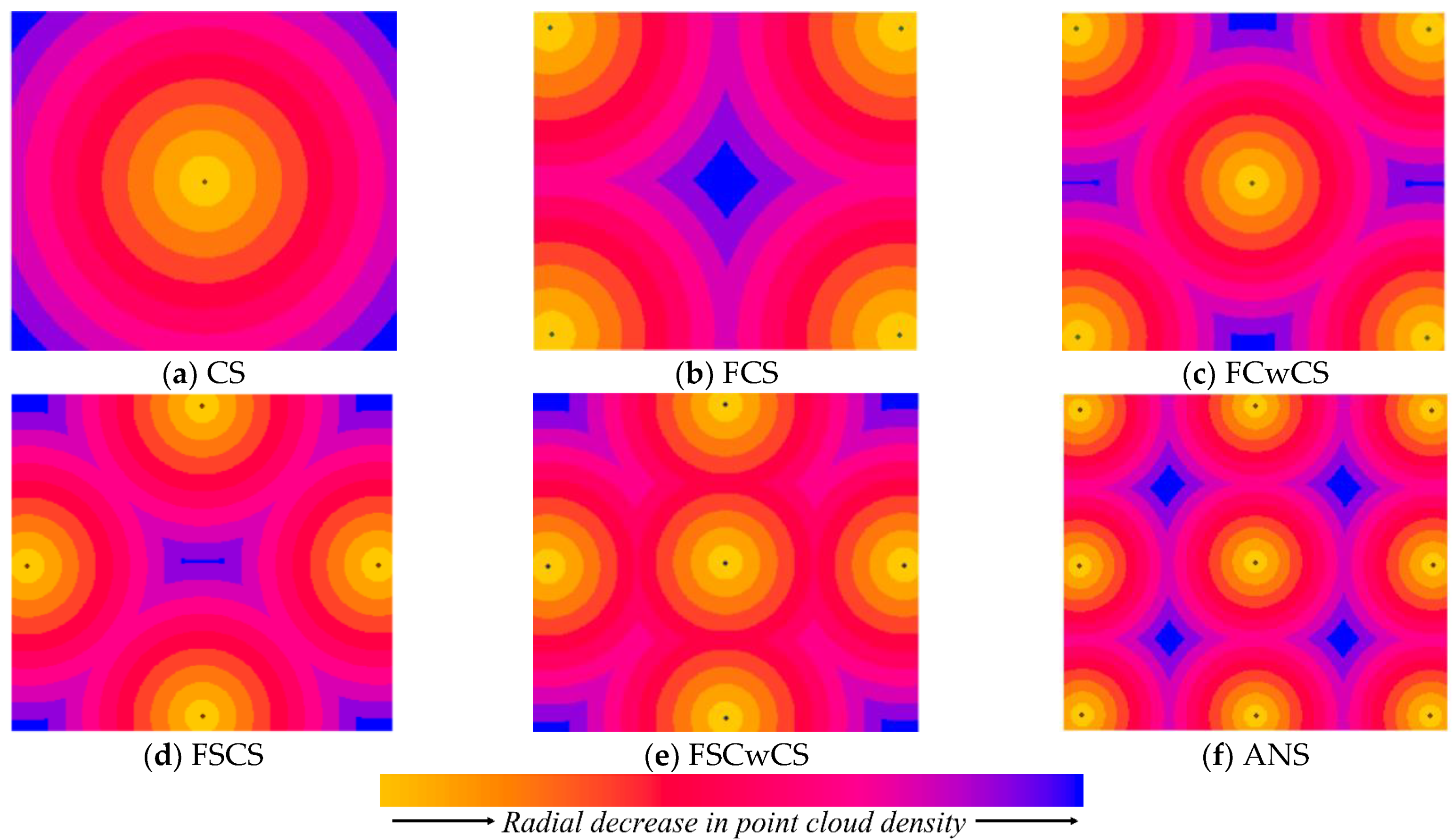
2.2.1. CS Combination

In this combination, only one scan position was considered, which was positioned at the center of the forest plot. As the scan was in the center, the TLS could collect the data in one complete sphere of influence. The sphere of influence is the imaginary region in which the TLS is capable of generating a point cloud (Figure 2).

2.2.2. FCS Combination

In this combination, four scan positions were considered, which were positioned at the four corners of the forest plot. The TLS scans were placed at the corners so that the scans could cover only 90° HFOV of the plot from each corner position, generating a point cloud in a quarter sphere of influence. Thus, all four scans at the corners could only contribute to one sphere of influence for the dataset when combined together.

2.2.3. FCwCS Combination

In this combination, five scan positions were considered. Four scans were placed at the four corners and one at the center of the forest plot. As the scans were placed at the corner and center, they could cumulatively contribute to two spheres of influence for the dataset. Four corners scans contribute to one sphere of influence, and the center scan contributes to one sphere of influence.

2.2.4. FSCS Combination

In this combination, four scan positions were considered. Which were placed at the center of all four sides. As each scan could cover only a 180° HFOV of the plot, they contributed to a half sphere of influence for the dataset. Therefore, a total of two spheres of influence for the dataset could be created in this combination.

2.2.5. FSCwCS Combination

In this combination, five scan positions were considered. Four scans from the center of each side and one at the center of the forest plot. Each side center scan contribute half of a sphere of influence, and the center scan contributes one complete sphere of influence. Therefore, a total of three spheres of influence for the dataset could be created with this combination.

2.2.6. ANS Combination

In this combination, nine scan positions were considered. Four scans were placed at the four corners, four other scans at the four side centers, and one at the center of the forest plot. The corner scans contribute to a quarter sphere of influence, the side center scans contribute half a sphere of influence, and the center scan contributes a complete sphere of influence. A total of four spheres of influence for the dataset could be created with this combination.
The theoretical representation of the patterns and positions of the TLS combinations followed for the data acquisition and processing are depicted in Figure 3; However, these behaved differently because of the standing trees in the forest plots. Hypothetically speaking, based on the theoretical maps from Figure 3, the combination FSCwCS should produce the most similar canopy top points to those of the ANS combination even with 4 fewer scan positions, as was observed for terrain points [22]. Further evaluation is needed to support or reject this hypothesis.
As the ANS scan combination had the highest number of scans and sphere of influence, the ANS scan combination was used as the reference dataset, which the other scan combination dataset was evaluated against. For visualization, the ANS scan combination point cloud datasets obtained for plots TLS_1a and TLS_2a are shown in Figure 4a,b, respectively.

2.3. Research Methodology

Six different TLS scan combination datasets were generated for each forest plot. Then, the canopy top points were extracted in each TLS scan combination, and a few canopy top points at the local grid of each tree stem position were clipped using the clipping tool in Cloudcompare [23]. Here, a local grid represents an imaginary region bounding the tree stem above which the canopy top points were extracted (Figure 6).
Multiple top points were extracted within the local grid for each combination. The highest point among these multiple points was considered the canopy top point for that particular combination at that local grid of that particular tree stem. These points were used for further analysis. Using the canopy top points extracted in the ANS scan combination as a reference, relative height differences with the canopy top points extracted in the other five scan combinations were calculated. The spatial analysis of relative height deviation was performed, and the results are shown in Figures 9 and 11. The research methodology followed throughout this research is represented as a workflow in Figure 5.

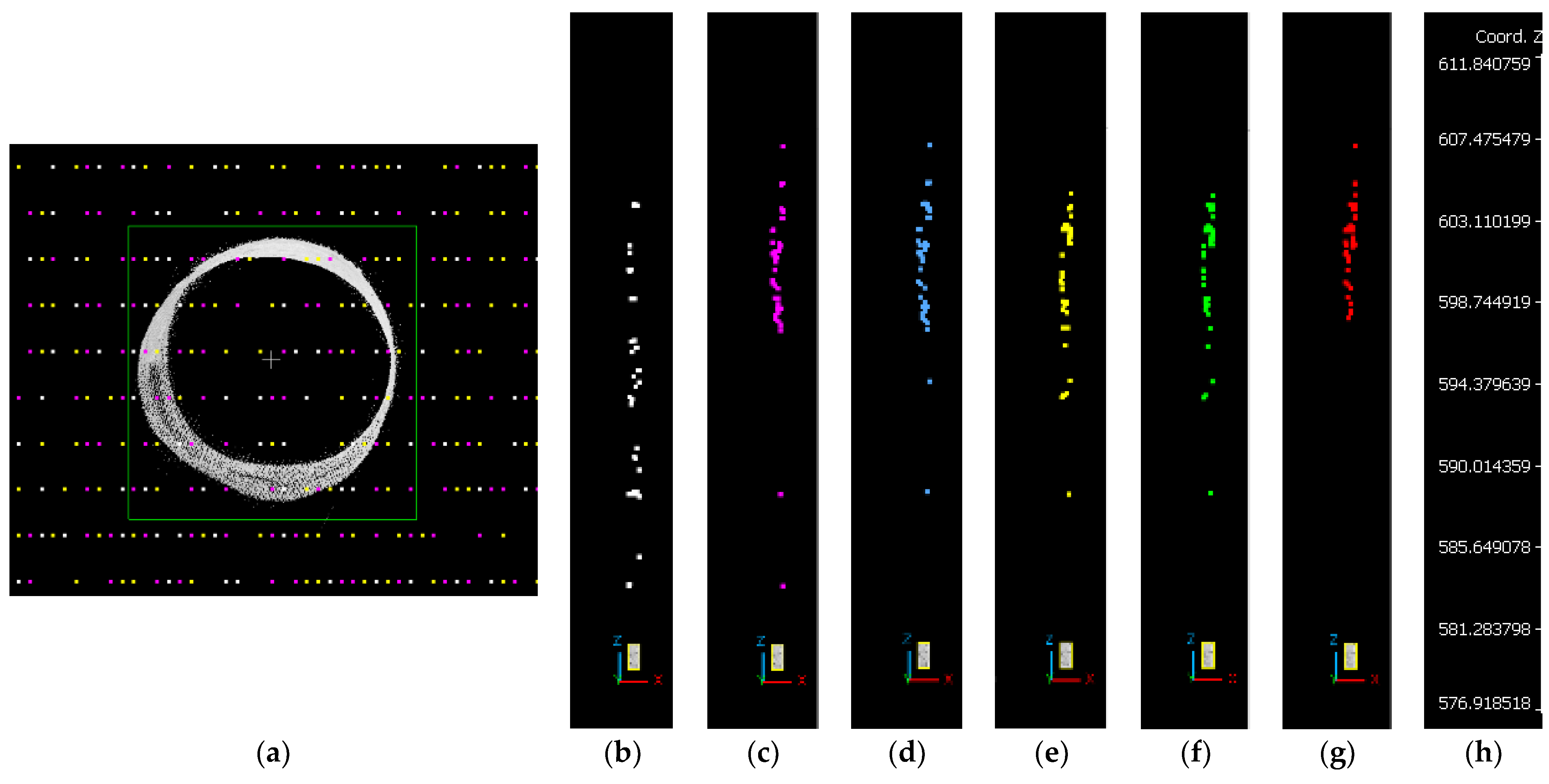
2.3.1. Canopy Top Points Extraction at Each Stem Local Grid Positions

The canopy top points were extracted in all the scan combinations for all eight forest plots in Dendrocloud [24]. The extract surface tool in the Dendrocloud software Version 1.53 was used to extract all the canopy surface points from the point cloud datasets with a grid size of 10 cm. The tool basically extracts the highest points within a cuboid region on the grid size mentioned as the canopy top point. The overall point cloud datasets are represented in the larger cuboid, and the canopy points extracted in a local cuboid region are shown in a smaller cuboid (base shown in blue) in Figure 6.
The canopy top points extracted from all the TLS scan combinations are shown for TLS_1a and TLS_2a in Figure 7a,b, respectively.
All the canopy top points obtained from all six combinations were opened together along with tree stems, and the point clouds were manually clipped to obtain the highest canopy point at that tree stem position. Then, the highest point in each canopy top point cloud at that tree stem position was used to represent the canopy top point at that tree stem position from all six TLS combinations (Figure 8). The canopy top points extracted at each stem grid position were used for spatial analysis of the variations in the heights between all the TLS scan combinations.

2.3.2. Data Evaluation

The point cloud data collected using TLS were divided into 6 TLS scan combinations for the plots in TLS_Plot1 and TLS_Plot2. Afterward, the relative elevation deviation between the canopy top points was calculated for each combination in the plots with respect to the ANS combination. Using all the combinations, we calculated the errors to evaluate the data.
The Root Mean Squared Error (RMSE), Mean Absolute Error (MAE), and relative Root Mean Squared Error (rRMSE) were calculated to compare the results obtained from the different combinations in the plots as shown in Equations (1)–(3), respectively.
RMSE = 1 N i = 1 N Y i Y ^ 2
MAE = 1 N i = 1 N Y i Y ^
rRMSE = 1 N i = 1 N Y i Y ^ 2 1 N i = 1 N Y i × 100
where,
  • Y i is the actual observation (m),
  • Y ^ is the estimated observation (m), and
  • N is the total number of observations.
To measure the statistical significance of all the combinations in terms of relative elevation deviation between the canopy top points and plot combinations, a two-way Analysis of Variance (ANOVA) was used. To identify the statistical significance of the difference between combinations, plots, and the relative elevation deviation between the canopy top points, Tukey post hoc tests were performed. The statistical analysis was conducted in R software.

3. Results

Spatial analysis and canopy top height differences for forest plot TLS_1a are presented in Section 3.1, forest plot TLS_2a is presented in Section 3.2, and forest plots TLS_1b, 1c 1d, 2b, 2c, and 2d are presented in Appendix A section.

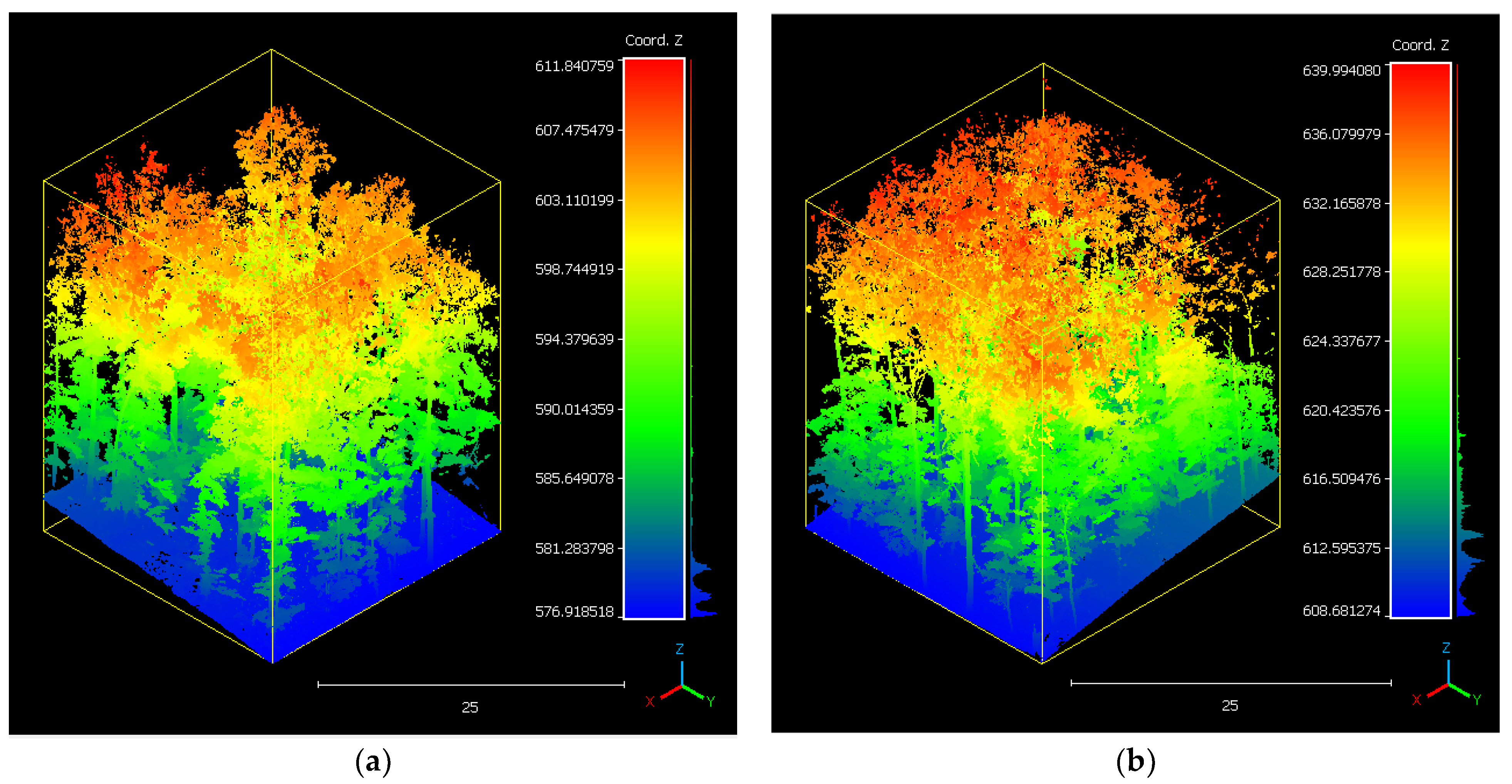
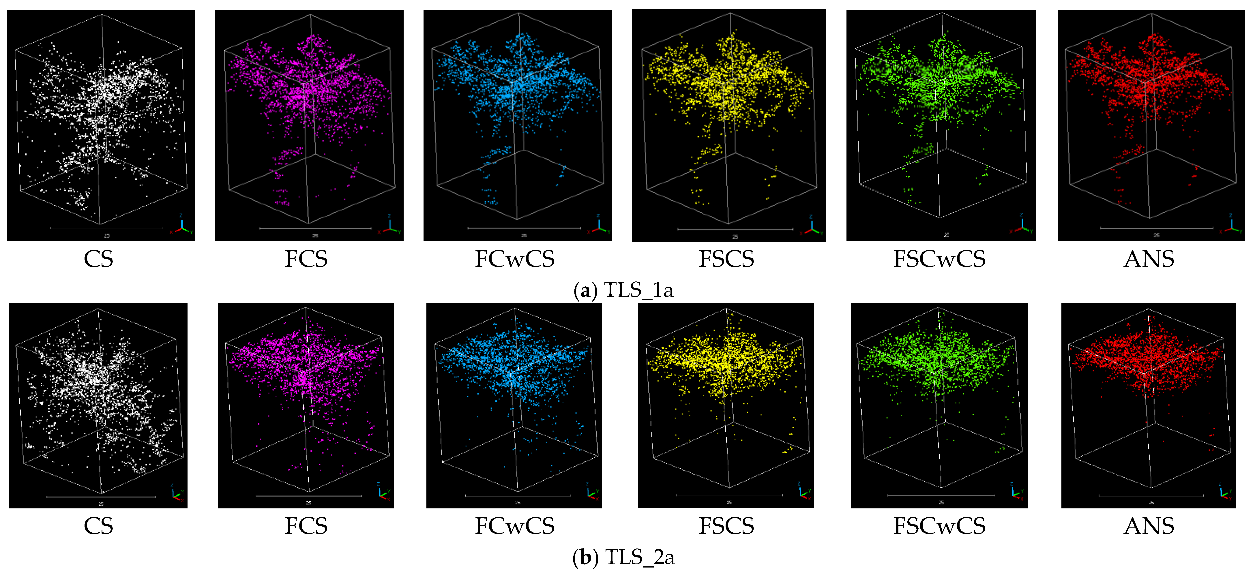
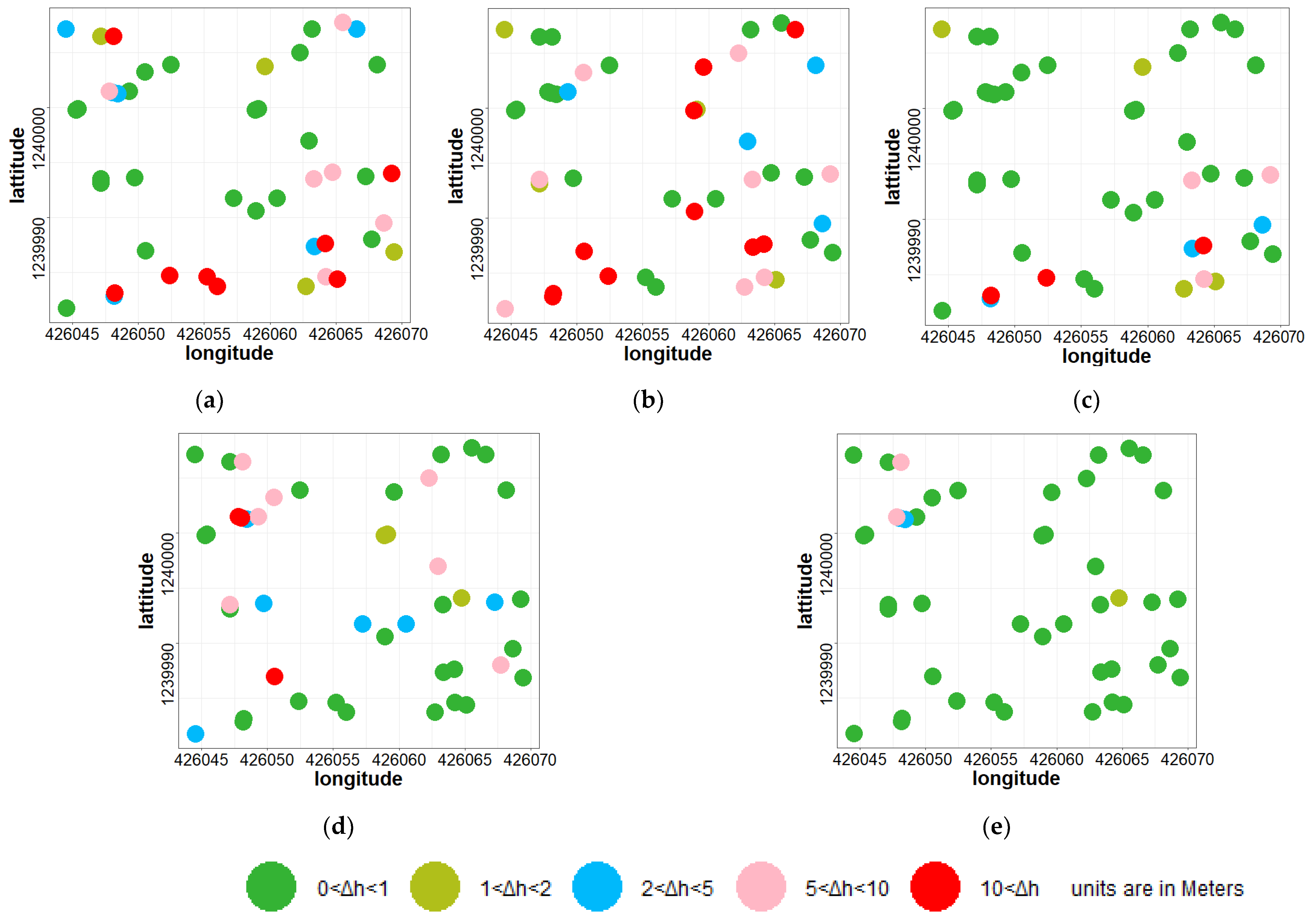
3.1. Spatial Analysis for Forest Plot TLS_1a

After the canopy top points extraction at each stem grid position in the forest plots for all the scan combinations, further analysis was conducted to observe the elevation deviation between the canopy top points in all the scan combinations with respect to the ANS scan combination at each tree stem position. The elevation deviations were spatially plotted to see the observations with reference to the spatial distribution along the plot. The plotting was based on the relative height deviation in meters; from 0 m to 1 m, 1 m to 2 m, 2 m to 5 m, 5 m to 10 m, and greater than 10 m are shown in dark green, light green, blue, light pink, and red colors, respectively. The maximum number of canopy points with an elevation difference of less than 1 m was generated with the FSCwCS combination, whereas the maximum canopy height difference of more than 10 m was observed in the CS combination. The spatial height deviations for plot TLS_1a are shown in Figure 9.

Canopy Top Height Differences for Forest Plot TLS_1a

The deviations in the relative spatial height difference between canopy top points in CS, FCS, FCwCS, FSCS, and FSCwCS with respect to the ANS scan combination for each tree in TLS_1a is shown as a graph in Figure 10.

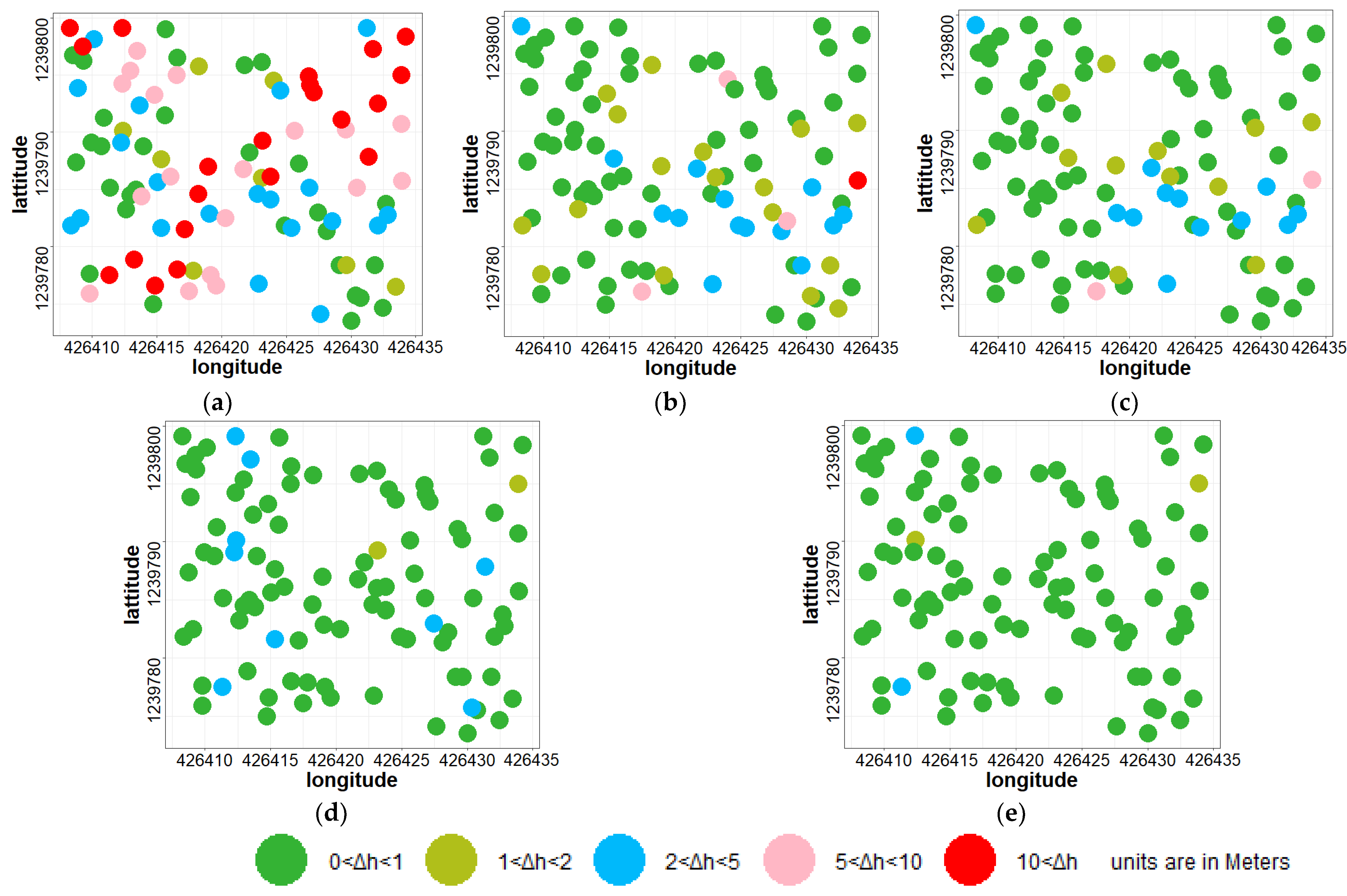
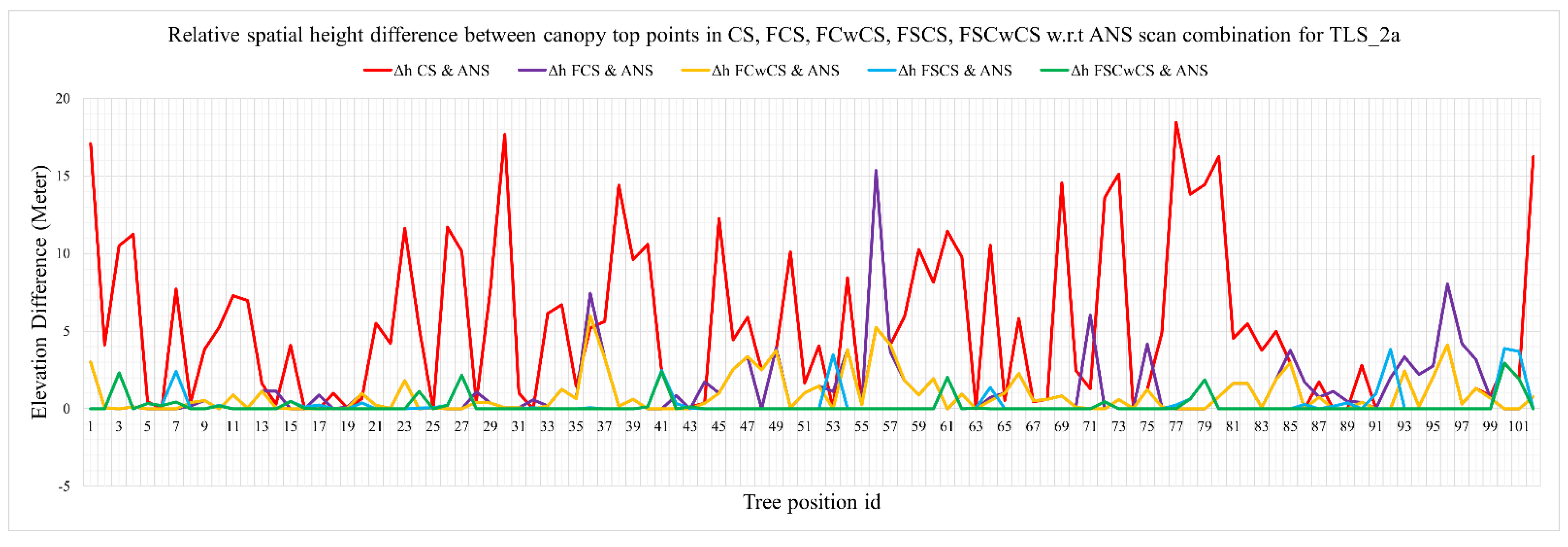
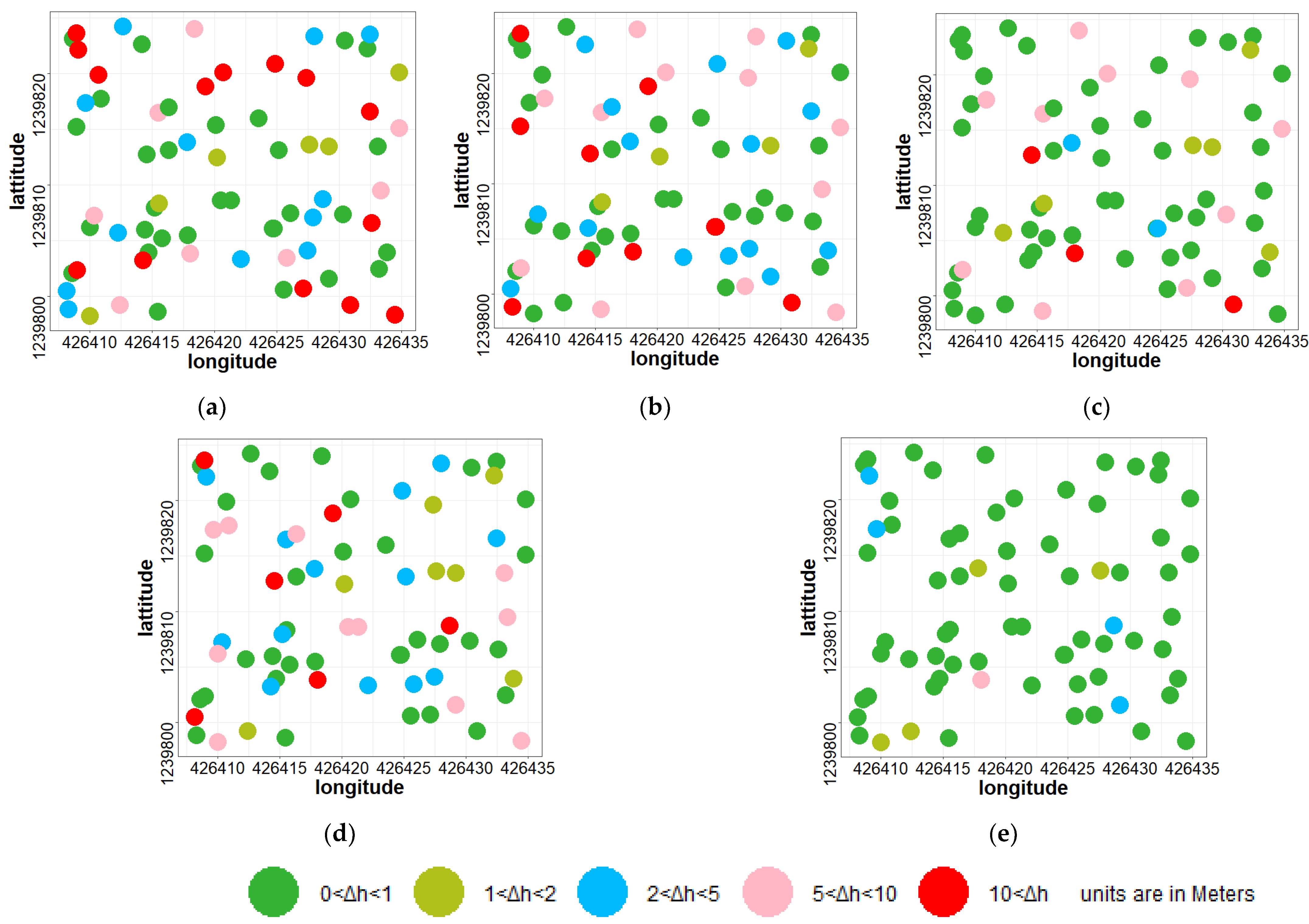
3.2. Spatial Analysis for Forest Plot TLS_2a

The spatial height difference between canopy top points obtained from each of the TLS scan combinations for forest plot TLS_2a with respect to the ANS scan combination at each tree stems position is shown in Figure 11. The maximum number of canopy points with an elevation difference of less than 1 m was generated with the FSCwCS combination, whereas the maximum number of canopy points with an elevation difference of more than 10 m was observed in the CS combination.

Spatial Canopy Top Height Differences for Forest Plot TLS_2a

The relative spatial height difference between canopy top points in CS, FCS, FCwCS, FSCS, and FSCwCS with respect to the ANS scan combination for each tree in TLS_2a is shown as a graph in Figure 12.

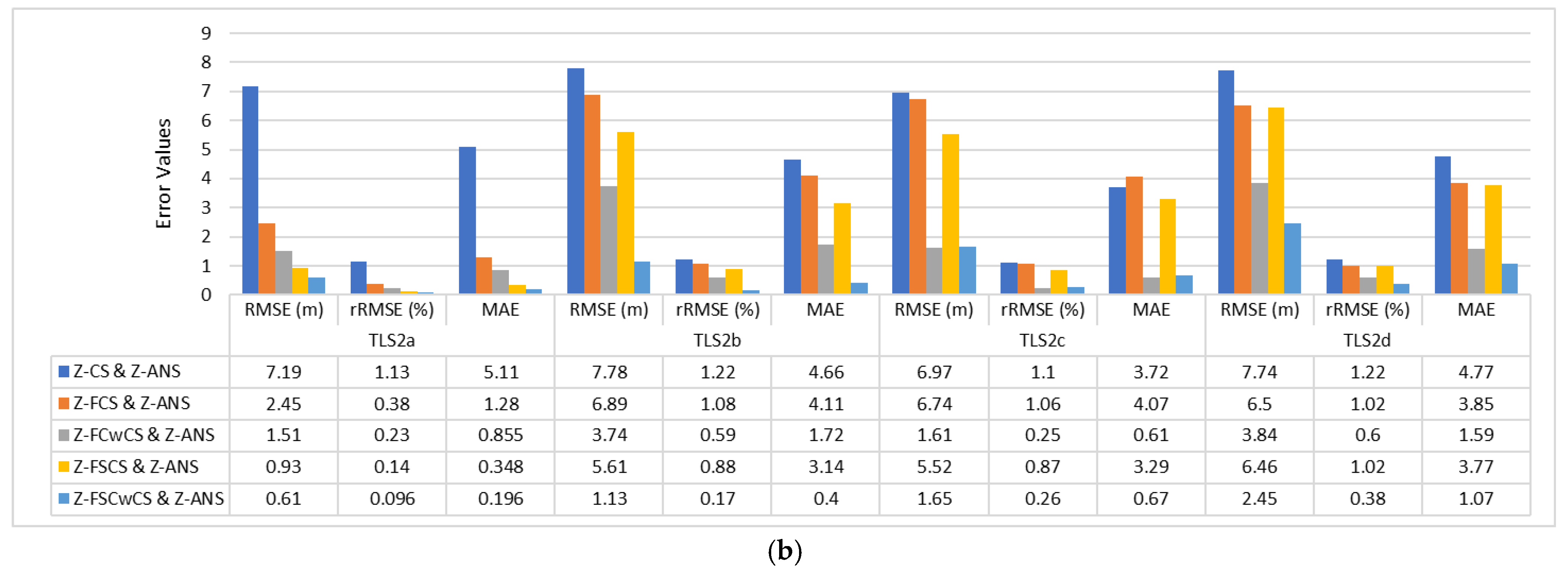
3.3. Qualitative Statistical Analysis for the Relative Canopy Heights

The relative elevation deviation between the canopy top points was calculated for each combination in the plots with respect to the ANS results in all the plots. Using the observation and analysis results obtained in the previous sections, the rRMSE was calculated. Statistical analysis was performed on the results obtained from the values computed from rRMSE. The rRMSE value obtained for TLS_Plot1 ranged from 0.15% to 2.48%. Overall, the combination of Z.FSCwCS and Z.ANS in TLS_1a showed the best results for the elevation deviation of the canopy points of trees in the respective plot.
The statistical error observed for TLS_Plot2 was analyzed. The scan combinations that came with the lowest error in the elevation difference of canopy points are Z.FSCwCS and Z.ANS for all the plots. The rRMSE values ranged between 0.096% and 1.22%. Overall, the TLS_2c plot with the combination of FSCwCS and ANS had the lowest error in the elevation differences of canopy points in all the trees among all the plots.
The rRMSE values obtained from all the relative canopy heights at each tree stem position from CS, FCS, FCwCS, FSCS, and FSCwCS with respect to the ANS scan combination for TLS_Plot1 and TLS_Plot2 are shown in Figure 13a,b.
Two-way ANOVA was performed considering different scan position combinations as one group and plots as another group to analyze the significant difference and impact on the relative elevation deviation of all combinations between the canopy top points among all the plots. It was performed to see whether there was any significant difference between the groups and within the group.
Hence, the relative elevation deviation of all combinations between the canopy top points among all the plots was significant at all tree stem positions. The scan combinations and their interactions with the plots were significantly impacting the relative elevation deviation of canopy top points. The ANOVA is shown in Table A1. Later, we performed a Tukey post hoc test to support ANOVA because we found a significant difference between the two groups (combinations and plots). So, due to the significant difference between these groups, the change in combinations of scan positions in the plot significantly affected the difference in the elevation of canopy points. Moreover, plots and combinations were significantly different from each other. When only combinations were compared, the Z.FCwCS-Z.ANS, Z.FSCwCS-Z.ANS, Z.FSCS-Z.FCS, and Z.FSCwCS-Z.FCwCS were not significant. When the Canopy Top Points Layer (CTPL) obtained from all plots was compared, CTPL_1c-CTPL_1b, CTP L_1d-CTPL_1c, and CTPL_2c-CTPL_2b were insignificant. To compare interactions, 1125 pairs were generated, out of which 732 pairs were significantly different from each other. The differences are depicted in Table A2 and Table A3.

4. Discussions

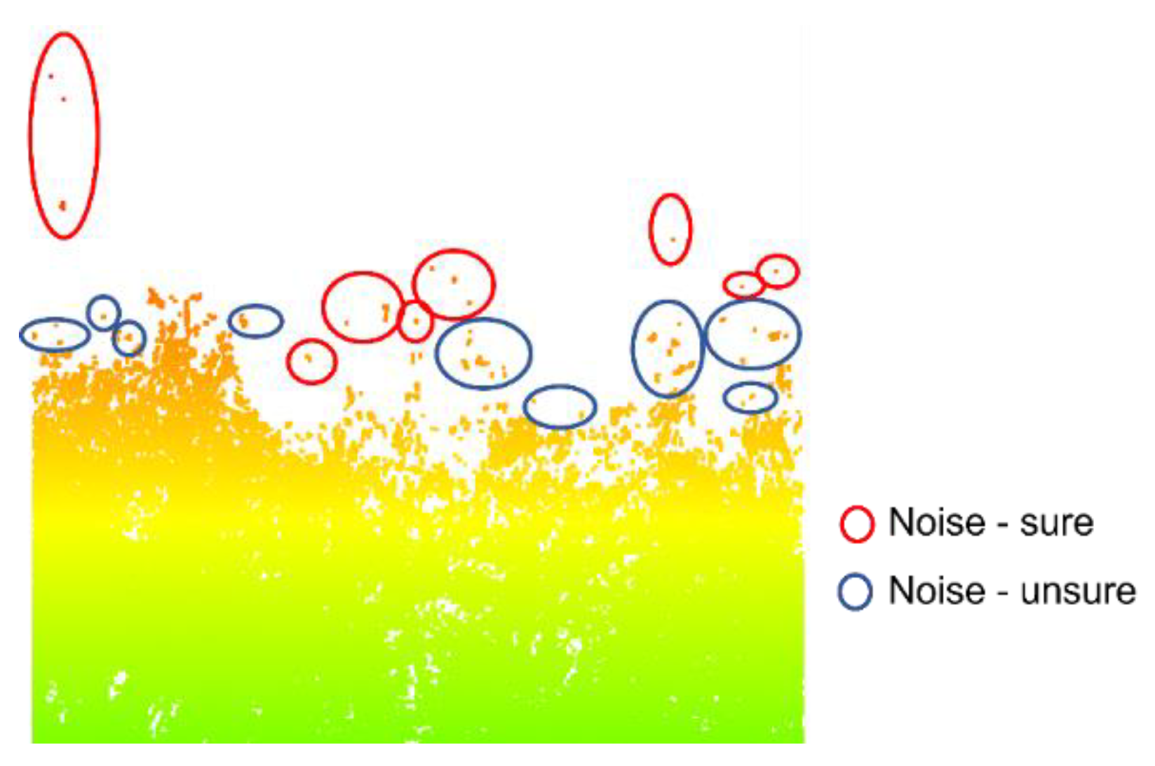
4.1. Noise Removal above the Canopy Regions

After merging the point clouds obtained from each TLS scan position, noise filtering is an important step, as noise can produce false results during canopy top points extraction. We have manually removed the noise as best as possible in this research using prior experience in point cloud data processing. However, we would like to present the situation of the points obtained at the canopy and above the canopy layer. Some points are too far from the canopy, which can easily be segmented out as noise, which is shown as sure noise points within red boundaries in Figure 14. Some points were close to the canopy and very sparsely dispersed. In this case, it is quite challenging to determine whether they are noise; they are shown as unsure noise points within violet boundaries in Figure 14. Since we are evaluating the canopy top points, it was critically important to segment out noise precisely. This was performed by observing the point cloud in different views and at small chunk levels to determine if a point is a noise.

4.2. Selection of Grid Size for Canopy Top Points Extraction in Dendrocloud

The canopy top points can be extracted at different grid sizes in Dendrocloud software. We have tried different grid sizes, and we came to a conclusion to extract the canopy top points using a 10cm grid size. If the grid size was more than 10 cm, the number of points being extracted was quite dense; similarly, if the grid size was less than 10 cm, the number of points being extracted was too low, which would not have served our purpose of extracting canopy top point at each tree stem position.

4.3. Highest Point Extraction at Each Tree Stem Position

The canopy top points at each tree stem position were manually extracted from all the TLS combinations from the canopy top layer points obtained from the process mentioned in Section 4.2. As the axis of the trees was not perpendicular for all the trees, there were some trees whose trunks were in between two plots which was a critical situation to consider; for example, there were some trees whose trunks were in one plot and the top in a different plot and there were also fallen trees whose branches were perpendicular which were falsely identified as individual trees, etc. With all these constraints under consideration, analyzing all eight plots and with six combinations was quite time-consuming. However, the accuracy of these extracted points was critical for the relative spatial analysis of the canopy top points at each tree stem position.

4.4. Effect of Number of Scans and Position of Scans on the Point Cloud Generation

In research carried out by Trochta J. et al., they found that the number of trees detected in a forest plot depended on the number of scanners and the close proximity of the trees to the scanner position. They tested tree detection in four scenarios with one scan, two scans, three scans, and four scans in different forest sites with different terrain undulations [25].Wan. P et al. conducted similar research to evaluate the efficiency of tree detection using TLS. However, they only used single scans in forests with three levels of densities and concluded that a single scan is only reliable for small forest plots that are less than 10 m in size [26].
In our research, we observed that the CS combination had the highest number of points with a relative height deviation greater than 10 m as the coverage of the TLS radially decreased towards the corners and edges of the plots. The combination of FSCwCS produced the least difference in canopy top points compared to the ANS combination, which we had predicted based on our previous work.

5. Conclusions

In this paper, we presented the statistical evaluation of the generation of point clouds at the top of the tree canopies in eight forest plots with varying tree densities using different TLS scan combinations. Different TLS scan positions have a varying penetration depth of the LiDAR beam through the dense canopy regions due to tree occlusions and various other factors. This aspect was evaluated with respect to the ANS scan combination, which was considered a reference scan combination for this research. The results in Section 3.1, Section 3.2 and Section 3.3 and Appendix A show that the Four Sides Center with Center Scans (FSCwCS) combination is quite efficient in producing canopy top points above the tree stem positions, similar to the ANS scan combination, which consists of nine TLS scanning positions. The deviation of the canopy top points was the lowest in the FSCwCS combination. Hence, the authors recommend that if the forest plots are around 25 m × 25 m in size, the FSCwCS combination can be considered for the optimum generation of canopy top surface points without increasing the time, number of scans, or size of the data.
In the future, we would like to test the quality of the DSM or CHM produced using different TLS scan combinations, as this research was based on point cloud-based analysis at the top points of the canopy at the location of each tree. It would be interesting to see the variation in the DSM or CHM surface at each pixel, including canopy top points, points above branches, and surface points in non-canopy regions.

Author Contributions

Conceptualization, Sunni Kanta Prasad Kushwaha and Arunima Singh; Methodology, Sunni Kanta Prasad Kushwaha and Arunima Singh; Software, Sunni Kanta Prasad Kushwaha; Validation, Sunni Kanta Prasad Kushwaha and Arunima Singh.; Formal analysis, Sunni Kanta Prasad Kushwaha; Investigation, Sunni Kanta Prasad Kushwaha and Martin Mokros; Resources, Martin Mokros and Kamal Jain; Data curation, Sunni Kanta Prasad Kushwaha and Martin Mokros; Writing—original draft preparation, Sunni Kanta Prasad Kushwaha, Arunima Singh and Martin Mokros; Writing—review and editing, Sunni Kanta Prasad Kushwaha, Arunima Singh, Jozef Vybostok and Martin Mokros; Visualization, Sunni Kanta Prasad Kushwaha; Supervision, Martin Mokros and Kamal Jain; Project administration, Martin Mokros; Funding acquisition, Jozef Vybostok and Martin Mokros. All authors have read and agreed to the published version of the manuscript.

Funding

This work was supported by grant No. CZ.02.1.01/0.0/0.0/16_019/0000803 (“Advanced research supporting the forestry and wood-processing sector’s adaptation to global change and the 4th industrial revolution”) financed by OP RDE, by the Scientific Grant Agency of the Ministry of Education, Science, Research, and Sport of the Slovak Republic and the Slovak Academy of Sciences [grant number VEGA 1/0335/20] and by the Slovak Research and Development Agency through Grant Nos. APVV-18-0305 and APVV-20-0391. The APC was funded by grant number VEGA 1/0335/20.

Data Availability Statement

Not applicable.

Acknowledgments

The authors would like to thank the anonymous reviewers for their thoughtful comments and suggestions on the original manuscript.

Conflicts of Interest

The authors declare no conflict of interest.

Appendix A

Appendix A.1. Statistical Errors Obtained for Plots TLS_Plot1 and TLS_Plot2

Figure A1. Graphs plots showing RMSE, MAE, and MSE for (a) TLS_Plot1, (b) TLS_Plot2.
Ijgi 12 00250 g0a1aIjgi 12 00250 g0a1b

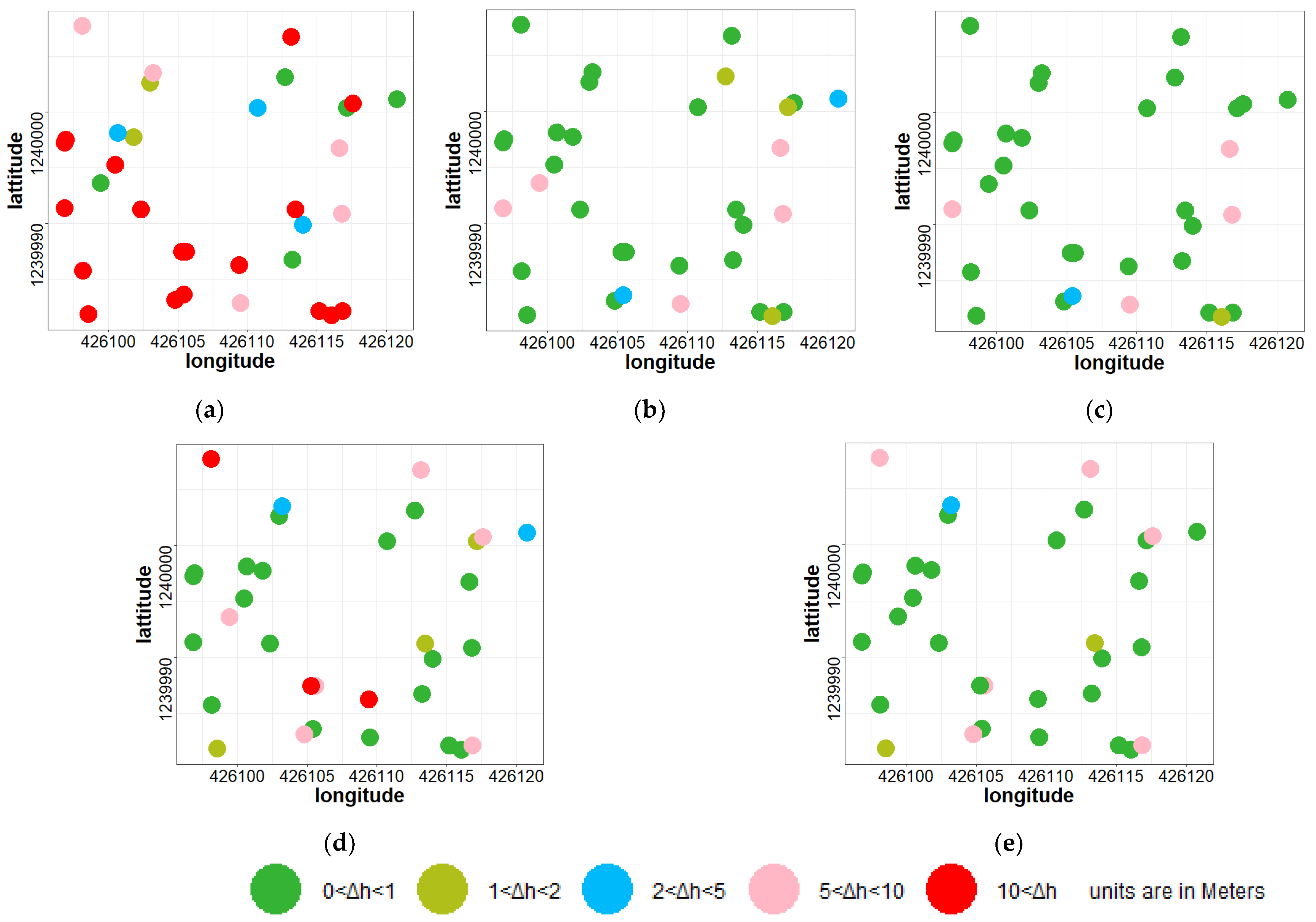
Appendix A.2. Spatial Analysis for Forest Plot TLS_1b

Figure A2. The spatial height differences between canopy top points obtained at each tree stem position in each of the TLS scan combinations for forest plot TLS_1b with respect to ANS scan combination. (a) Δh CS and ANS; (b) Δh FCS and ANS; (c) Δh FCwCS and ANS; (d) Δh FSCS and ANS; (e) Δh FSCwCS and ANS.
Ijgi 12 00250 g0a2

Spatial Canopy Top Height Differences for Forest Plot TLS_1b

Figure A3. Graph showing relative spatial height differences between canopy top points in CS, FCS, FCwCS, FSCS, and FSCwCS with respect to ANS scan combination for TLS_1b.
Ijgi 12 00250 g0a3

Appendix A.3. Spatial Analysis for Forest Plot TLS_1c

Figure A4. The spatial height differences between canopy top points obtained at each tree stem position in each of the TLS scan combinations for forest plot TLS_1c with respect to ANS scan combination. (a) Δh CS and ANS, (b) Δh FCS and ANS, (c) Δh FCwCS and ANS, (d) Δh FSCS and ANS, and (e) Δh FSCwCS and ANS.
Ijgi 12 00250 g0a4

Spatial Canopy Top Height Differences for Forest Plot TLS_1c

Figure A5. Graph showing relative spatial height differences between canopy top points in CS, FCS, FCwCS, FSCS, and FSCwCS with respect to ANS scan combination for TLS_1c.
Ijgi 12 00250 g0a5

Appendix A.4. Spatial Analysis for Forest Plot TLS_1d

Figure A6. The spatial height differences between canopy top points obtained at each tree stem position in each of the TLS scan combinations for forest plot TLS_1d with respect to ANS scan combination. (a) Δh CS and ANS, (b) Δh FCS and ANS, (c) Δh FCwCS and ANS, (d) Δh FSCS and ANS, and (e) Δh FSCwCS and ANS.
Ijgi 12 00250 g0a6

Spatial Canopy Top Height Differences for Forest Plot TLS_1d

Figure A7. Graph showing relative spatial height differences between canopy top points in CS, FCS, FCwCS, FSCS, and FSCwCS with respect to ANS scan combination for TLS_1d.
Ijgi 12 00250 g0a7

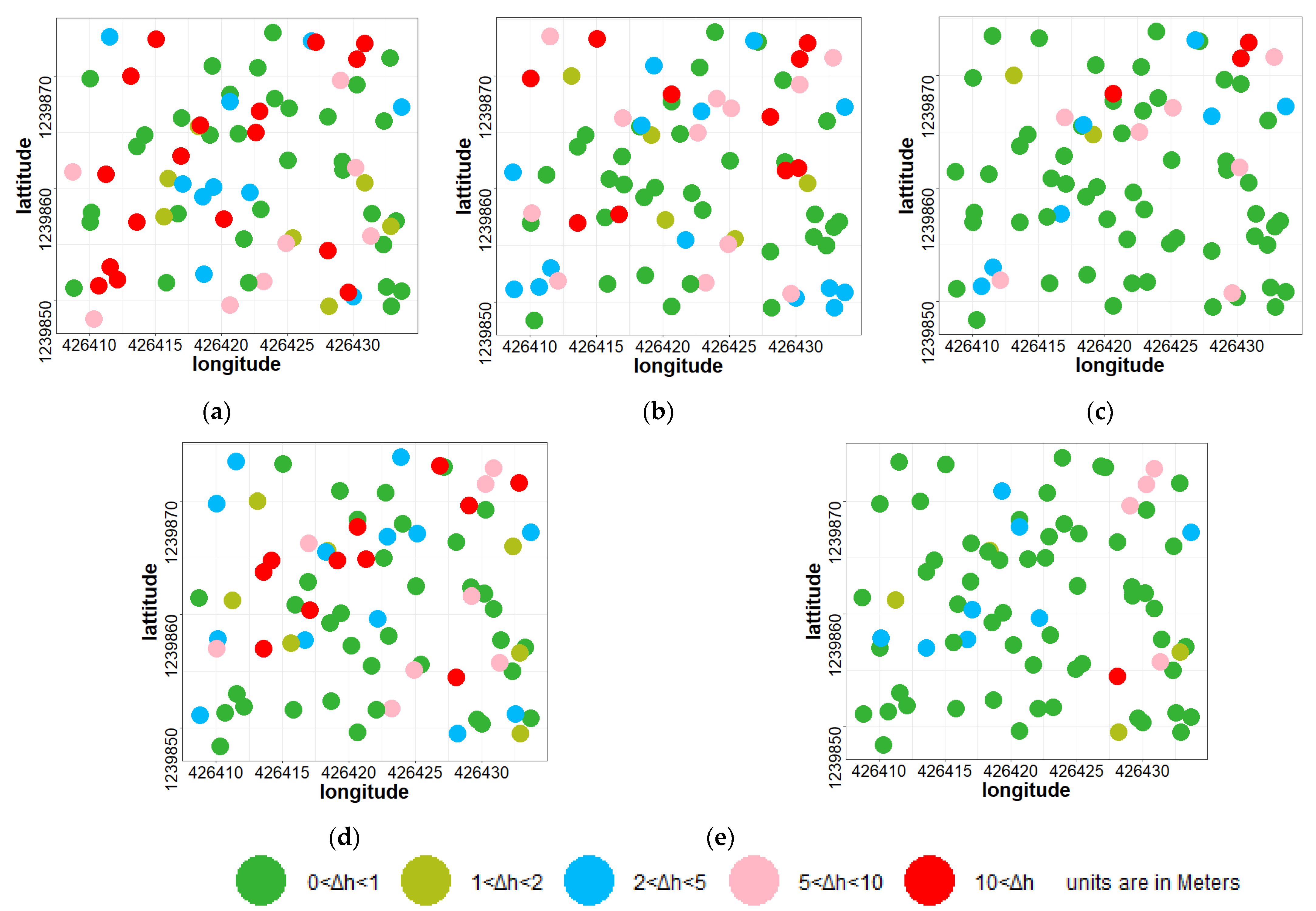
Appendix A.5. Spatial Analysis for Forest Plot TLS_2b

Figure A8. The spatial height differences between canopy top points obtained at each tree stem position in each of the TLS scan combinations for forest plot TLS_2b with respect to ANS scan combination. (a) Δh CS and ANS, (b) Δh FCS and ANS, (c) Δh FCwCS and ANS, (d) Δh FSCS and ANS, and (e) Δh FSCwCS and ANS.
Ijgi 12 00250 g0a8

Spatial Canopy Top Height Differences for Forest Plot TLS_2b

Figure A9. Graph showing relative spatial height differences between canopy top points in CS, FCS, FCwCS, FSCS, and FSCwCS with respect to ANS scan combination for TLS_2b.
Ijgi 12 00250 g0a9

Appendix A.6. Spatial Analysis for Forest Plot TLS_2c

Figure A10. The spatial height differences between canopy top points obtained at each tree stem position in each of the TLS scan combinations for forest plot TLS_2c with respect to ANS scan combination. (a) Δh CS and ANS, (b) Δh FCS and ANS, (c) Δh FCwCS and ANS, (d) Δh FSCS and ANS, and (e) Δh FSCwCS and ANS.
Ijgi 12 00250 g0a10

Spatial Canopy Top Height Differences for Forest Plot TLS_2c

Figure A11. Graph showing relative spatial height differences between canopy top points in CS, FCS, FCwCS, FSCS, and FSCwCS with respect to ANS scan combination for TLS_2c.
Ijgi 12 00250 g0a11

Appendix A.7. Spatial Analysis for Forest Plot TLS_2d

Figure A12. The spatial height differences between canopy top points obtained at each tree stem position in each of the TLS scan combinations for forest plot TLS_2d with respect to ANS scan combination. (a) Δh CS and ANS, (b) Δh FCS and ANS, (c) Δh FCwCS and ANS, (d) Δh FSCS and ANS, and (e) Δh FSCwCS and ANS.
Ijgi 12 00250 g0a12

Spatial Canopy Top Height Differences for Forest Plot TLS_2d

Figure A13. Graph showing relative spatial height differences between canopy top points in CS, FCS, FCwCS, FSCS, and FSCwCS with respect to ANS scan combination for TLS_2d.
Ijgi 12 00250 g0a13
Table A1. Analysis of variance results.
S.no.TermsDfSum SqMean SqF ValuePr (>F)
1Combination59171183467.015<2 × 10⁻¹⁶ ***
2Plot7577,37082,4813013.445<2 × 10⁻¹⁶ ***
3Combination: Plot353057873.1911.04 × 10−9 ***
4Residuals287478,66527NANA
Signif. codes: 0 ‘***’; 0.001 ‘**’; 0.01 ‘*’; 0.05 ‘.’; 0.1 ‘ ’ 1.
Table A2. Tukey post hoc test results for multiple comparisons of means of combinations.
TermsCombination. diffCombination. lwrCombination. uprCombination.p.adj
Z.CS-Z.ANS5.321615678−6.277687548−4.3655438090
Z.FCS-Z.ANS−3.110681938−4.066753807−2.1546100690
Z.FCwCS-Z.ANS−1.21057849−2.166650359−0.254506620.004199711
Z.FSCS-Z.ANS−2.217747268−3.173819137−1.2616753990
Z.FSCwCS-Z.ANS−0.609996896−1.5660687650.3460749730.453265265
Z.FCS-Z.CS2.210933741.2548618713.1670056090
Z.FCwCS-Z.CS4.1110371893.154965325.0671090580
Z.FSCS-Z.CS3.103868412.1477965414.0599402790
Z.FSCwCS-Z.CS4.7116187833.7555469135.6676906520
Z.FCwCS-Z.FCS1.9001034490.944031582.8561753182.37 × 10−7
Z.FSCS-Z.FCS0.89293467−0.0631371991.8490065390.083054818
Z.FSCwCS-Z.FCS2.5006850431.5446131733.4567569120
Z.FSCS-Z.FCwCS−1.007168779−1.963240648−0.051096910.032108868
Z.FSCwCS-Z.FCwCS0.600581594−0.3554902751.5566534630.471492715
Z.FSCwCS-Z.FSCS1.6077503720.6516785032.5638222412.52 × 10−5
Table A3. Tukey post hoc test results for multiple comparisons of means by the plot.
TermsPlot. diffPlot. lwrPlot. uprPlot.p.adj
CTPL_1b-CTPL_1a−1.24421−2.581790.0933760.090111
CTPL_1c-CTPL_1a−1.50771−2.98012−0.035290.040289
CTPL_1d-CTPL_1a−3.27041−4.72927−1.811560
CTPL_2a-CTPL_1a30.4907129.3646731.616740
CTPL_2b-CTPL_1a27.9147326.7149929.114480
CTPL_2c-CTPL_1a28.3272327.1463229.508140
CTPL_2d-CTPL_1a26.5438725.3569827.730760
CTPL_1c-CTPL_1b−0.2635−1.761551.2345450.999483
CTPL_1d-CTPL_1b−2.02621−3.51093−0.541480.000935
CTPL_2a-CTPL_1b31.7349130.5755732.894260
CTPL_2b-CTPL_1b29.1589427.9278730.390010
CTPL_2c-CTPL_1b29.5714428.3587230.784160
CTPL_2d-CTPL_1b27.7880826.5695329.006620
CTPL_1d-CTPL_1c−1.7627−3.36996−0.155450.020074
CTPL_2a-CTPL_1c31.9984130.685833.311030
CTPL_2b-CTPL_1c29.4224428.0460730.798820
CTPL_2c-CTPL_1c29.8349428.4749531.194930
CTPL_2d-CTPL_1c28.0515826.6863929.416760
CTPL_2a-CTPL_1d33.7611232.4637335.058510
CTPL_2b-CTPL_1d31.1851529.8232932.547010
CTPL_2c-CTPL_1d31.5976430.2523532.942940
CTPL_2d-CTPL_1d29.8142828.4637331.164830
CTPL_2b-CTPL_2a−2.57597−3.57314−1.57880
CTPL_2c-CTPL_2a−2.16347−3.1379−1.189050
CTPL_2d-CTPL_2a−3.94684−4.9285−2.965170
CTPL_2c-CTPL_2b0.412498−0.646251.4712470.937254
CTPL_2d-CTPL_2b−1.37087−2.43628−0.305450.002467
CTPL_2d-CTPL_2c−1.78336−2.82752−0.73926.54 × 10−6

References

  1. Singh, A.; Kushwaha, S.K.P.; Nandy, S.; Padalia, H. An approach for tree volume estimation using RANSAC and RHT algorithms from TLS dataset. Appl. Geomat. 2022, 14, 785–794. [Google Scholar] [CrossRef]
  2. Yu, H.; Yang, W.; Xia, G.S.; Liu, G. A color-texture-structure descriptor for high-resolution satellite image classification. Remote Sens. 2016, 8, 259. [Google Scholar] [CrossRef] [Green Version]
  3. Forbes, B.; Reilly, S.; Clark, M.; Ferrell, R.; Kelly, A.; Krause, P.; Matley, C.; O’Neil, M.; Villasenor, M.; Disney, M.; et al. Comparing Remote Sensing and Field-Based Approaches to Estimate Ladder Fuels and Predict Wildfire Burn Severity. Front. For. Glob. Chang. 2022, 5, 818713. [Google Scholar] [CrossRef]
  4. Calders, K.; Adams, J.; Armston, J.; Bartholomeus, H.; Bauwens, S.; Bentley, L.P.; Chave, J.; Danson, F.M.; Demol, M.; Disney, M.; et al. Terrestrial laser scanning in forest ecology: Expanding the horizon. Remote Sens. Environ. 2020, 251, 112102. [Google Scholar] [CrossRef]
  5. Chen, J.; Chen, Y.; Liu, Z. Extraction of Forestry Parameters Based on Multi-Platform LiDAR. IEEE Access 2022, 10, 21077–21094. [Google Scholar] [CrossRef]
  6. Cabo, C.; Ordóñez, C.; López-Sánchez, C.A.; Armesto, J. Automatic dendrometry: Tree detection, tree height and diameter estimation using terrestrial laser scanning. Int. J. Appl. Earth Obs. Geoinf. 2018, 69, 164–174. [Google Scholar] [CrossRef]
  7. Kankare, V.; Puttonen, E.; Holopainen, M.; Hyyppä, J. The effect of TLS point cloud sampling on tree detection and diameter measurement accuracy. Remote Sens. Lett. 2016, 7, 495–502. [Google Scholar] [CrossRef]
  8. Åkerblom, M.; Kaitaniemi, P. Terrestrial laser scanning: A new standard of forest measuring and modelling? Ann. Bot. 2021, 128, 653–662. [Google Scholar] [CrossRef]
  9. García, M.; Danson, F.M.; Riaño, D.; Chuvieco, E.; Ramirez, F.A.; Bandugula, V. Terrestrial laser scanning to estimate plot-level forest canopy fuel properties. Int. J. Appl. Earth Obs. Geoinf. 2011, 13, 636–645. [Google Scholar] [CrossRef]
  10. Disney, M. Terrestrial LiDAR: A three-dimensional revolution in how we look at trees. New Phytol. 2019, 222, 1736–1741. [Google Scholar] [CrossRef] [Green Version]
  11. Walter, J.A.; Stovall, A.E.L.; Atkins, J.W. Vegetation structural complexity and biodiversity in the Great Smoky Mountains. Ecosphere 2021, 12, e03390. [Google Scholar] [CrossRef]
  12. Wilkes, P.; Lau, A.; Disney, M.; Calders, K.; Burt, A.; Gonzalez de Tanago, J.; Bartholomeus, H.; Brede, B.; Herold, M. Data acquisition considerations for Terrestrial Laser Scanning of forest plots. Remote Sens. Environ. 2017, 196, 140–153. [Google Scholar] [CrossRef]
  13. Wezyk, P.; Koziol, K.; Glista, M.; Pierzchalski, M. Terrestrial laser scanning versus traditional forest inventory first results from the polish forests. In Proceedings of the ISPRS Workshop on Laser Scanning 2007 and SilviLaser 2007, Espoo, Finland, 12–14 September 2007; Volume 36, pp. 424–429. [Google Scholar]
  14. Palace, M.; Sullivan, F.B.; Ducey, M.; Herrick, C. Estimating Tropical Forest Structure Using a Terrestrial Lidar. PLoS ONE 2016, 11, e0154115. [Google Scholar] [CrossRef] [PubMed] [Green Version]
  15. Decuyper, M.; Mulatu, K.A.; Brede, B.; Calders, K.; Armston, J.; Rozendaal, D.M.A.; Mora, B.; Clevers, J.G.P.W.; Kooistra, L.; Herold, M.; et al. Assessing the structural differences between tropical forest types using Terrestrial Laser Scanning. For. Ecol. Manag. 2018, 429, 327–335. [Google Scholar] [CrossRef]
  16. Azuan, N.H.; Khairunniza-Bejo, S.; Abdullah, A.F.; Kassim, M.S.M.; Ahmad, D. Analysis of Changes in Oil Palm Canopy Architecture from Basal Stem Rot Using Terrestrial Laser Scanner. Plant Dis. 2019, 103, 3218–3225. [Google Scholar] [CrossRef] [PubMed] [Green Version]
  17. Muumbe, T.P.; Tagwireyi, P.; Mafuratidze, P.; Hussin, Y.; van Leeuwen, L. Estimating above-ground biomass of individual trees with terrestrial laser scanner and 3D quantitative structure modelling. South. For. 2021, 83, 56–68. [Google Scholar] [CrossRef]
  18. Seidel, D.; Fleck, S.; Leuschner, C.; Hammett, T. Review of ground-based methods to measure the distribution of biomass in forest canopies. Ann. For. Sci. 2011, 68, 225–244. [Google Scholar] [CrossRef] [Green Version]
  19. Pueschel, P. The influence of scanner parameters on the extraction of tree metrics from FARO Photon 120 terrestrial laser scans. ISPRS J. Photogramm. Remote Sens. 2013, 78, 58–68. [Google Scholar] [CrossRef]
  20. Abegg, M.; Kükenbrink, D.; Zell, J.; Schaepman, M.E.; Morsdorf, F. Terrestrial laser scanning for forest inventories-tree diameter distribution and scanner location impact on occlusion. Forests 2017, 8, 184. [Google Scholar] [CrossRef] [Green Version]
  21. Gollob, C.; Ritter, T.; Wassermann, C.; Nothdurft, A. Influence of scanner position and plot size on the accuracy of tree detection and diameter estimation using terrestrial laser scanning on forest inventory plots. Remote Sens. 2019, 11, 1602. [Google Scholar] [CrossRef] [Green Version]
  22. Kushwaha, S.K.P.; Singh, A.; Jain, K.; Mokros, M. Optimum Number and Positions of Terrestrial Laser Scanner To Derive Dtm At Forest Plot Level. Int. Arch. Photogramm. Remote Sens. Spat. Inf. Sci.-ISPRS Arch. 2022, 43, 457–462. [Google Scholar] [CrossRef]
  23. CloudCompare. [GPL Software] Vrsion 2.12.4. 2022. Available online: https://www.danielgm.net/cc/release/ (accessed on 24 February 2023).
  24. Koren, M. Dendrocloud Version 1.53. Available online: https://gis.tuzvo.sk/dendrocloud/download.aspx (accessed on 24 February 2023).
  25. Trochta, J.; Král, K.; Janík, D.; Adam, D. Arrangement of terrestrial laser scanner positions for area-wide stem mapping of natural forests. Can. J. For. Res. 2013, 43, 355–363. [Google Scholar] [CrossRef]
  26. Wan, P.; Wang, T.; Zhang, W.; Liang, X.; Skidmore, A.K.; Yan, G. Quantification of occlusions influencing the tree stem curve retrieving from single-scan terrestrial laser scanning data. For. Ecosyst. 2019, 6, 43. [Google Scholar] [CrossRef] [Green Version]
Figure 1. Study area map depicting the location of TLS_Plot1 and TLS_Plot2.
Ijgi 12 00250 g001
Figure 2. (a) Diagram of a TLS with its 360° Horizontal Field of View (HFOV) and 320° Vertical Field of View (VFOV), and the region of data generation is its sphere of influence. (b) Image of the TLS instrument in one of the forest plots.
Ijgi 12 00250 g002
Figure 3. Theoretical representation of TLS scan positions and their spheres of influence in all six scan combination patterns. (a) Center Scans (CS), (b) Four Corners Scans (FCS), (c) Four Corners with Center Scans (FCwCS), (d) Four Sides Center Scans (FSCS), (e) Four Sides Center with Center Scans (FSCwCS), and (f) All Nine Scans (ANS)—The ANS combination was used as a reference.
Ijgi 12 00250 g003
Figure 4. ANS scan combination point cloud datasets for plots (a) TLS_1a and (b) TLS_2a.
Ijgi 12 00250 g004
Figure 5. Research methodology.
Ijgi 12 00250 g005
Figure 6. Diagram showing the grid size with respect to to the plot size in which the highest points were extracted to identify canopy top points in each TLS scan combination.
Ijgi 12 00250 g006
Figure 7. Canopy top points obtained in each TLS scan combination for forest plots (a) TLS_1a, (b) TLS_2a.
Ijgi 12 00250 g007
Figure 8. (a) Image representing canopy top points from all six combinations and a tree stem within a local grid (shown as a green bounding box) in which the canopy top points were extracted corresponding to the tree stem (top view). Canopy top points extracted above the tree stem for (b) CS shown in white, (c) FCS shown in pink, (d) FCwCS shown in blue, (e) FSCS shown in yellow, (f) FSCwCS shown in green, (g) ANS shown in red (front view), and (h) scale bar for points shown in (bg).
Ijgi 12 00250 g008
Figure 9. The spatial height differences between canopy top points obtained at each tree stem position in each of the TLS scan combinations for forest plot TLS_1a with respect to ANS scan combination. (a) Δh CS and ANS, (b) Δh FCS and ANS, (c) Δh FCwCS and ANS, (d) Δh FSCS and ANS, and (e) Δh FSCwCS and ANS.
Ijgi 12 00250 g009
Figure 10. Graph showing relative spatial height differences between canopy top points in CS, FCS, FCwCS, FSCS, and FSCwCS with respect to ANS scan combination for each tree in TLS_1a.
Ijgi 12 00250 g010
Figure 11. The spatial height differences between canopy top points obtained at each tree stem position from each of the TLS scan combinations for forest plot TLS_2a with respect to ANS scan combination. (a) Δh CS and ANS, (b) Δh FCS and ANS, (c) Δh FCwCS and ANS, (d) Δh FSCS and ANS, and (e) Δh FSCwCS and ANS.
Ijgi 12 00250 g011
Figure 12. Graph showing relative spatial height differences between canopy top points in CS, FCS, FCwCS, FSCS, and FSCwCS with respect to ANS scan combination for TLS_2a.
Ijgi 12 00250 g012
Figure 13. Graph plots showing rRMSE for (a) TLS_Plot1 and (b) TLS_Plot2.
Ijgi 12 00250 g013aIjgi 12 00250 g013b
Figure 14. Shows a close-up front view of the forest point cloud at the canopy level, which shows sure noise points in red boundaries and unsure noise points in violet boundaries.
Ijgi 12 00250 g014
Table 1. Number of trees in each of the four subplots for both research plots TLS_Plot1 and TLS_Plot2.
TLS_Plot1TLS_Plot2
SubplotsNumber of TreesSubplotsNumber of Trees
TLS_1a49TLS_2a102
TLS_1b45TLS_2b72
TLS_1c32TLS_2c78
TLS_1d33TLS_2d76
Disclaimer/Publisher’s Note: The statements, opinions and data contained in all publications are solely those of the individual author(s) and contributor(s) and not of MDPI and/or the editor(s). MDPI and/or the editor(s) disclaim responsibility for any injury to people or property resulting from any ideas, methods, instructions or products referred to in the content.

